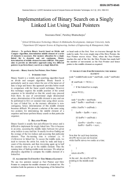
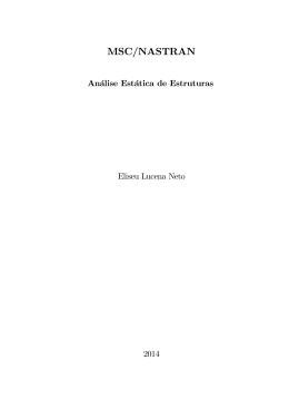
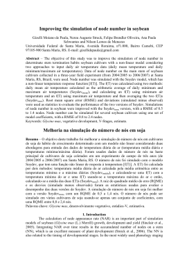
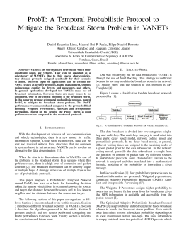
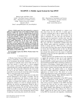
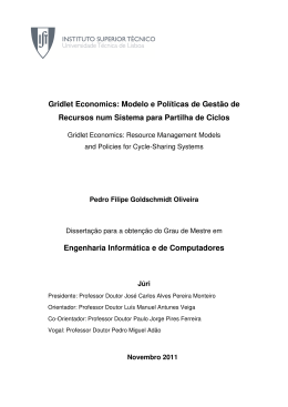
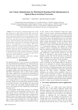
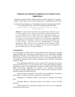
IAT'2005 - The 2005 IEEE/WIC/ACM International Conference on Intelligent Agent Technology
Dynamic Determination of the Itinerary of Mobile Agents
with Timing Constraints
Luciana Rech
LCMI-DAS-UFSC
[email protected]
Romulo Silva de Oliveira
LCMI-DAS-UFSC
[email protected]
Abstract
The mobile agent technology is an important research
area in the scope of code mobility. As part of an agent
mission objective, it may exist the necessity of meeting an
end-to-end deadline, although with some flexibility about
the itinerary the agent should follow. The objective of this
paper is to define an execution model for mobile agents
that include timing constraints. We also show some
simple heuristics that are able to guide these agents in the
itinerary definition, considering the existence of an endto-end deadline for the mission.
1. Introduction
Within the context of code mobility, an important
research area is the mobile agents technology [1, 2]. A
mobile agent is an element of self-contained software that
is responsible for the execution of a task, and that is not
limited to the system where it starts execution. It is able to
migrate in an autonomous way through the network. A
mobile agent must be able to interrupt its execution in a
place, to move to another one, and to retake its execution
there. Mobile agents reduce the load in the network. They
execute in a way both assynchronous and autonomous,
and they can dynamically adapt, thus establishing a new
paradigm for the programming in distributed
environments. An important requirement that can be
associated to mobile agents is the timing aspect.
A possible scenario that illustrates the use of mobile
agents with time constraints is a system of generation and
distribution of electrical power where, by following a
hierarchic structure, the data is widely spread physically.
In the context of the electrical power industry, a wide
geographic scale and response in real- time are only two
requirements for the supervision and control system,
which is also characterized by the heterogeneity of the
equipment. The scale of this type of system can be of
thousand of nodes [3].
Considering a power generating plant and the
substations that take part in the electrical power
transmission, the mobile agent can substitute the
technician (or engineer), with his laptop, visiting section
Carlos Montez
LCMI-DAS-UFSC
[email protected]
by section of the system. The agent has as function: to
collect data, to form an image of the problem and to
decide the next visit for collection of data. The diagnosis
of a fault is achieved by visiting some nodes and by
collecting data for the decision taking.
This paper deals with code mobility in a distributed
system associated with timing constraints. Its objective is
to define an execution model for applications based on
imprecise mobile agents with real time constraints. Also,
this paper presents some basic algorithms for dynamic
determination of itinerary. An imprecise mobile agent is
able to negotiate the quality of the result in order to meet
the mission deadline.
This text is divided in 6 sections. In section 2 we
review some previous work found in the literature related
to this subject. In section 3 the adopted execution model is
described. In section 4 it is introduced some simple
heuristics for the definition of the itinerary. Section 5
presents a comparison of this heuristics and section 6 has
the conclusions.
2. Related Work
There are some previous work in the literature about
the agents technology and time constraints. In [4] is
described a routing system based on agents (ARS - Agentbased Routing System) that allocates network resources
for tasks that requested point-to-point real-time
communication. Mobile agents are supported by a
resource management mechanism, they collect current
link status of the system to examine the availability of
possible routes to each node.
Another work that associates timing constrains to
mobile agents is [5], where the decision taking is
implemented through negotiation between intelligent and
independent mobile agents. A negotiation protocol based
on mobile agents (MANPro) is applied for real-time
scheduling of a production line system.
The RT Monitor is a real-time data management
system that deals with traffic data for applications in
network navigation [6]. Navigation requests with timing
constraints are originated and the RT Monitor calculates
and communicates the best routes to the requesting tasks.
IAT'2005 - The 2005 IEEE/WIC/ACM International Conference on Intelligent Agent Technology
The precision of the suggested routes depends on the
consistency of the traffic data. To minimize the overhead,
a distributed cooperative method is adopted using mobile
agents, aiming at to improve system scalability and to
reduce communication traffic.
BAEK et.al. in [2] consider a method for planning of
mobile agents with timing constraints (TMAP - Timed
Mobile Agent Planning) in order to find the minimum
number of agents and the best itinerary for agents to
recovery information in a distributed computation
environment. They must respect the timing constraints
while keeping the minimum total routing time.
Among the above works, only in [2] there is the
concern of choosing an itinerary where timing constraints
are respected. However, in the execution model
considered in this paper, there is the concern of choosing
the best itinerary considering the performance of the task
execution and the difficulty in meeting the deadline. In
this context, the definition of "best" itinerary may vary, in
accordance with the metric used to evaluate itineraries.
Adaptive scheduling techniques will be used to establish a
compromise between the visits to nodes and the timing
constraints of the mission.
The imprecise computation [7], for example, is a
technique able to establish a solid conceptual base for the
decisions that will be made by the agent and/or the
support system, with respect to its scheduling. The
itinerary of the mobile agent must be constructed so as all
the mandatory resources are executed. Moreover, it
should execute optional resources so as to maximize the
value added to the mission of the agent, without missing
the end-to-end deadline.
The problem considered in this work is also similar to
that presented in [8], entitled "The prize collecting
traveling salesman problem". However, algorithms as
presented in [8, 9] are computationally expensive and
directed toward the static determination of the itinerary,
when there are no real-time constraints.
3. Execution Model
The proposed execution model describes the behavior
of an application based on mobile agents, with timing
constraints, in a distributed system, formed by a set of
nodes connected through a communication underlying
service. In this execution model, each mobile agent has a
mission. The mission is described in terms of the visit to a
determined set of nodes, which includes the necessary
resources for the agent. It is assumed that this agent does
not communicate with other agents. The agent mission is
formed by a task set that will be executed respecting a
single deadline. A task represents the use of a resource by
the agent in a node.
A resource is an abstraction and can correspond to a
processor, device, file, data structure, etc. Each resource
has an associated benefit that is derived from its
functional importance for the mission. In each system
node there is a set of resources. There can be many
instances of the same type of resource in distinct nodes.
The processor is always a necessary resource for the agent
and it is presented in every node. So, it will be treated
implicitly.
The itinerary is the route defined by a sequence of
nodes. Each agent in our model has some flexibility for
defining its itinerary. This flexibility comes from the
resources that can: i) to be used in any order, ii) to appear
duplicated, iii) to be discarded or iv) to be partially used
(with respect to its utilization time).
3.1. Problem Formulation
A computational system is characterized by a set N of
nodes and a set R of resources types. The set N of nodes
of the system has cardinality m, that is, it is composed by
m nodes Ni, Ni / N, where 1 ” i ” m.
In each node Ni of the system there is a set Ri of one or
more types of resources of the set R. Each type of
resource of set R can be found in one or more nodes, that
is, there can be many instances (duplicates) of a same type
of resource, as long as they are in distinct nodes. The
Figure 1 illustrates a situation where it is possible to
observe that instances of the resource type r3 appear in
node N2 and in node N6.
communication network
Node 1 Node 2 Node 3 Node 4 Node 5 Node 6
r1, r2
r3, r4
r1
r5, r6
r7, r8
r3
Figure 1. Resources in nodes of a distributed system
An itinerary I is defined as a route in a computational
system, it is described as a node sequence Ni pertaining to
the set N. An itinerary does not need to include all the
nodes of the system, and it may include in its sequence
the same node more that one time.
Each mobile agent Z has a mission M that defines a
benefit function B for each type of resource. This function
determines how much of benefit Bi each type of resource
ri contributes to the agent individual mission.
The agent has as objective to add benefits through the
use of resources spread among nodes interconnected by a
communication network. The objective function of the
agent is to maximize the collected total benefit throughout
its itinerary in the system. The agent starts at system
external node N0 (origin node) and must come back to it
at the end of the mission. The node N0 does not has
instances of the types of resources that form the set R. It is
IAT'2005 - The 2005 IEEE/WIC/ACM International Conference on Intelligent Agent Technology
assumed clock synchronization in the system. Every
mission M has a firm deadline D associated.
The agent Z must conclude the mission (and to return
to node N0) before D, or it will lose all the benefit
collected along its itinerary.
The resource diagram of a mission M (Figure 2)
corresponds to an UML activity diagram that describes
the existing precedence relations about the use of
resources. Any resource used in disagreement with this
diagram adds no benefit to the mission.
r0
r1<<variable>>
The flexibility in composing the itinerary is associated
with the resources of set R, since some of them may be
used without a previously defined order (for instance: r5
and r3 in Figure 2), may appear duplicated (for instance:
r1 in N1 and N3, in Figure 1), may be discarded (for
instance: r7 in Figure 2) or may be used partially (for
instance: r1, in Figure 2).
The node diagram of a mission M corresponds to an
UML activity diagram constructed from the resource
diagram of mission M, where each resource is substituted
by the node or nodes where it appears in the system. This
diagram presents the set of all possible itineraries for the
agent. For example, assuming that the mission described
in Figure 2 was executed in the system described in
Figure 1, Figure 3 contains the resultant node diagram of
this mission, and it represents the possibility of different
itineraries that the agent can follow to conclude its
mission.
r2
N0
r3
r5
r4
N1<<variable>>
N3<<variable>>
r6
N1
r8
r7
N2
N6
N4
N2
r0
N4
Figure 2. Resource diagram of a mission M
The resource diagram of the mission describes the
flexibility and the agent options when carrying through
the mission. Figure 2 describes a mission where eight
resources are used. Resource type r0 is a pseudo-resource,
only found in node N0, it is used to indicate the agent
must return to the original node. In the diagram, the
stereotype <<variable>> indicates that the time of usage
of resource r1 is variable, it may be released before the
agent gets its maximum benefit.
N5
N0
Figure 3. Node diagram of a mission M
IAT'2005 - The 2005 IEEE/WIC/ACM International Conference on Intelligent Agent Technology
The execution of mission M can be seen as an
aperiodic activity A. An activity is defined as the task set
X and network latencies L that compose an itinerary I in
particular. A task xi represents the use of a resource ri by
an agent Z in a node Ni. Each task xi belongs to set X. The
activations of these tasks (x1, x2, ..., xn. where n =
cardinality of set X) occur in irregular intervals of time,
characterizing the aperiodical aspect of the activity and
the tasks. The deadline D of the activity A is associated
with the conclusion of all the tasks that belong to activity
A.
The conclusion of a mission M depends on the choice
of an itinerary I. The definition of the itinerary should
take into account: i) the time of computation for
maximum benefit of each task xi, called Ci; ii) the
communication latency between nodes Nk and Ny, called
Ly; iii) the dependences between the resources that appear
in the resource diagram of the mission.
It should be considered the cost for an agent to arrive
at a node (coming from the previous node) and to acquire
the resource (Ki + Qi where: Ki is the execution time in the
node and Qi is the waiting time at the local processor).
For all ri / R, the benefit Bi,t collected for using the
resource ri during the interval of time t is showed by:
1) ri at the variable type
Bi,t = Bi x min (1, t/Ci)
[1]
where Bi is the collected maximum benefit of ri
and Ci is the maximum computation time associated with
ri (Ci is the time interval that the agent must hold the
resource to gain Bi and t is the time interval that the agent
actually holded it).
2) ri the normal type
Bi,t = Bi
Bi,t = 0
se t
se t
•C
C
[2]
i
i
For the equations above we must consider optionality
and precedence relations:
- if ri precedes rj, and ri was not used, then Bj=0;
- if ri' and ri" are duplicates of ri, and ri’ was already
used, then the maximum benefit of ri“ becomes zero.
The effective benefit of the mission is defined as the
sum of the benefits collected from each resource along the
itinerary:
B = ∑ Bi(y)
for every ri
Ý R.
[3]
where Bi(y) is the benefit collected by using resource ri
that the agent visited when following the itinerary y, B is
the benefit generated for the use of all the resources of the
mission.
4. Algorithms for definition of the itinerary
This section presents some simple heuristics, that can
be used with the execution model presented in this work.
These simple heuristics make their decisions based only
on the data associated with the possible immediate nodes
to visit, it does not consider the future unfolding of their
short term decisions. When the agent needs to decide
between two routes that, in the perspective of the used
heuristic, are equivalent, it takes a random decision.
4.1. Lazy Algorithm
The lazy algorithm tries to execute all resources as
quickly as possible. It ignore the benefit of each resource.
The optional resources are not executed, and resources
with stereotype <<variable>> are executed during the
minimum possible time. When there are alternative
routes, it will choose the one that has the minimum
execution time, that is, when there is no precedence
relation between two resources, it will be chosen the
resource that presents the smallest computation time.
Thus, the collected benefit will be minimum, even zero
sometimes. In the case of the existence of duplicates of a
resource, initially it is verified if there is an instance of
this resource in the node where the agent is at the moment
(the node where it used the previous resource). In
negative case, it will choose the closest node to visit.
4.2. Greedy Algorithm
Every time that there is an alternative, the greedy
algorithm will choose the one that generates the greatest
benefit. For example, when there is no precedence
relation between two resources, it will choose the resource
that presents the greatest benefit for the mission. This
algorithm always executes optional nodes. In cases where
the resource is of type <<variable>>, the greedy algorithm
executes the requested time to get the maximum benefit.
Like the previous algorithm, in case of the existence of
duplicated resources, the preference is for the resource
situated in the nearest node.
4.3. Random Algorithm
This algorithm randomly chooses the next node to be
visited by the agent. This behavior is only possible if there
are duplicates of one resource or there is no precedence
relation between the next resource and some of the others
resources to be used. When the resource is of type
<<variable>>, the random algorithm will decide randomly
between zero and the computation time necessary to
collect the maximum benefit from this resource.
IAT'2005 - The 2005 IEEE/WIC/ACM International Conference on Intelligent Agent Technology
4.4. Higher Density Algorithm
The higher density algorithm - based on policy AVDT
(Average Density Threshold) [10] - chooses as the next
resource to be executed the one that presents the best
relation benefit/time. This is only possible when there is
no precedence relation between two resources. The
density of the resource benefit is defined by the equation:
dbi = Bi / ( Ci + Lj,i +Qi)
where: dbi = density of the benefit of resource i, Bi =
benefit collected from the execution of resource i, Ci =
time of computation used for resource i, Lj,i = time
necessary to move to node Ni, and Qi = waiting time at the
local processor. Estimated values can be used when the
actual ones are not known.
The agent keeps the average value db observed until
the current moment. When a resource is optional, it will
only be executed if its density is bigger than the mean
density of the mission until that moment.
Observing the table, we notice that the greedy algorithm
with clock does not execute the optional resource r8
(respecting the mission deadline), with the purpose of
keeping the total benefit collected so far.
When the random algorithm is used (and observing the
diagram of Figure 3), a possible itinerary is: N3, N1, N4,
N2, N4, N5. As the criterion of decision used to choose the
next resource is random, there are many possible
itineraries.
Observing the diagram of Figure 3 and the resultant
itinerary (Table 1), it was estimated the relation between
the collected benefit and the time expended to get this
benefit for each resource (E1=10/10, E2=3/2, E3=3/7,
E4=7/2, E5=5/8, E6=3/5, E7=6/7, E8=8/3).
According to table 1: Alg1 represents Lazy Algorithm;
Alg2, Greedy Algorithm; Alg3, Random Algorithm;
Alg4, Higher Density Algorithm; Alg5, Greedy with
clock; Alg6, Random with clock; and Alg7 Higher
Density with clock.
Table 1. Comparison of the itinerary definition algorithms
4.5. Versions with Clock
A possible variation of the above algorithms is to
estimate the time necessary to execute the remaining
mandatory resources of the mission, before deciding the
next resource to be executed. The existing slack is
calculated by the difference between the deadline and the
execution time of the mandatory resources, added to the
time necessary to move the agent between nodes.
Optional resources will only be executed if the slack is
big enough. This estimate can be applied to the algorithms
already described, with the exception of the lazy
algorithm, that is not affected by it.
Alg
1
Alg
2
Alg
3
Alg
4
5. Comparison of the Heuristics
Table 1 presents a comparison of the performance of
the described algorithms using the system example of
section 3. For the calculation of the mission total
computation time, the computation time of each resource
has been considered and a fixed time of communication L
between the nodes (L=1).
In the presented models the diagrams of Figures 2 and
3 will be considered, along with the computation times
(t1=10, t2=2, t3=7, t4=2, t5=8, t6=5, t7=7, t8=3) and the
benefits (B1=10, B2=3, B3=3, B4=7, B5=5, B6=3, B7=6,
B8=8). In this study we assume that the communication
and computation times are previously known by the agent.
The variable resources have minimum execution time
equal to zero.
In this example, the total benefit of the mission when
using the greedy algorithm with deadline 50 was 0, since
that is a firm deadline and total computation time was 51.
Alg
5
Alg
6
Alg
7
Itinerary D=20 D=30 D=40
N1, N6, T=29 T=29 T=29
N2, N4 N4 B=0 B=21 B=21
(21)
N1, N1, T=51 T=51 T=51
N4, N6,
B=0 B=0 B=0
N2, N4,
(45) (45) (45)
N 5, N 5
N3, N1, T=48 T=48 T=48
N4, N2,
B=0 B=0 B=0
N2, N4,
(37) (37) (37)
N5
N1, N1, T=43 T=43 T=43
N4, N2 N4, B=0 B=0 B=0
(39) (39) (39)
N5
N1, N1, T=30 T=30 T=40
N4, N6,
B=0 B=21 B=31
N2, N4,
(21)
N5
N3, N1, T=29 T=29 T=37
N4, N2,
B=0 B=21 B=28
N2, N4,
(21)
N5, N5
N1, N1, T=29 T=30 T=39
N4, N2 N4, B=0 B=22 B=31
(21)
N5
D=50 D=60
T=29 T=29
B=21 B=21
T=51
B=0
(45)
T=51
B=45
T=48
B=37
T=48
B=37
T=43
B=39
T=43
B=39
T=48
B=37
T=51
B=45
T=48
B=42
T=48
B=42
T=43
B=39
T=43
B=39
When using the Higher Density Algorithm, through the
analysis of the relations B/Ci, we notice that the agent
executed r5 before r3. As the average density of the
mission until the moment of the execution of r7 and r8 was
Em = 1,275 and the densities of the optional resources r7
IAT'2005 - The 2005 IEEE/WIC/ACM International Conference on Intelligent Agent Technology
and r8 are E7=0,85 and E8=2,67 respectively, only
optional resource r8 was executed.
The Figure 4 shows the algorithms behavior
considering the collected benefits. Observing the graphic,
it can be noticed that, among the algorithm versions
without clock, the Lazy Algorithm is the only one that
obtained benefit with deadlines very short (for instance:
D=30). The algorithm versions with clock deal better with
short deadlines if compared with the ones without clock.
When larger deadlines are defined, the biggest benefits
are collected by the greedy algorithm, considering both
versions (with and without clock).
Figure 4. Comparison among the itinerary definition
algorithms
6. Conclusions
This paper defined an execution model for imprecise
mobile agents with time constraints and some flexibility
in the definition of its itinerary. The paper also described
some simple heuristics that can be used by the mobile
agent for the process of choosing the itinerary. Although
simple, the heuristics presented can be used as a starting
point for more complex algorithms. The execution model
presented here is innovative in associating time
constraints and the concept of optional resources to the
technology of mobile agents.
A comparison between the heuristics showed that there
is a necessity to establish a compromise between mission
value and execution time. As future work we include the
study of more elaborate algorithms for this problem, by
combining characteristics of several of the simple
heuristics presented here. Also, a performance evaluation
considering the probabilistic behavior of network and
nodes is necessary.
7. Acknowledgements
The authors would like to thank CNPQ (Counsel
National of Development Scientific and Techonological)
by the financial support that allowed the realization of this
work.
8. References
[1] Picco, G. P., “Understanding, Evaluating, Formalizing, and
Exploiting Code Mobility”. Doctor Thesis. Politecno di
Torino, Italy, 1998.
[2] Baek, J.W., Kim, G.T., and Yeom, H.Y., “Timed Mobile
Agent Planning for Distributed Information Retrieval”
Engineering and Computation School. Seoul National
University. Proceedings of AGENTS´01. Montreal,
Quebec, Canada, June, 2001.
[3] Tolbert, L.M., Qi, H, and Peng, F. Z., “Scalable Multi-Agent
System for Real-Time Electric Power Management”
IEEE Power Engineering Society Summer Meeting.
Vancouver, Canada, July, 2001, pp. 1676-1679.
[4] Oika, K., and Sekido, M., “ARS: An efficient agent-based
routing system for QoS guarantees” Elsevier Science,
Computer Communications 23, pp. 1437-1447. 2000.
[5] Shin, M., Jung, M, and Riu, K., “A Novel Negotiation
Protocol for Agent-based Control Architecture” 5th Int.
Conference on Engineering & Automation. Las Vegas,
USA, 2001.
[6] Ramamritham, K., Kwan, A., and Lam, K.Y, “RTMonitor:
Real-time Data Monitoring Using Mobile Agent
Technologies” Proceedings of 28th VLDB Conference,
Hong Kong, China, 2002.
[7] Liu, J. W. S., Shih, W.-K., Lin, K.-J., et al. “Imprecise
Computations” Proceedings of the IEEE, Vol. 82. nº 1,
January, 1994, pp. 83-94.
[8] Balas, E. “The Prize Collecting Traveling Salesman
Problem” John Wiley & Sons, Inc. Networks, Vol.19,
1989, pp.621-636.
[9] Balas, E. “The Prize Collecting Traveling Salesman
Problem: II” Polyhedral Results. John Wiley & Sons,
Inc. Networks, Vol.25, 1995, pp.199-216.
[10] Davis, A., et al., “Flexible Scheduling for Adaptable RealTime Systems” Proc. IEEE Real-Time Tech. and App.
Symp, May, 1995.