Lab 5 - Part D
Bar Plots & Dot Plots
Bar and dot plots are used in two ways: (1) to display proportions of categories, and (2) to compare class
means, i.e. experimental treatments or sampling sites. In either case, you don’t have a sensible scale on
your x-axis, i.e. your independent variable is a factor, such as “Control”, “Nitrogen”, “Phosphorus”,
“Nitrogen & Phosporous” fertilization. Because the bars/dots can be grouped, these graph types work well
for factorial experiments with multiple treatments (or for hierarchical sampling designs).
5.15. Bar charts for factorial designs

We are already familiar with a dataset from a factorial experiment, our lentil data from Lab 2 on data
tables and data management. Let’s set up as usual with a new folder, an empty workspace shortcut
to start R. Then load, check, and attach the dataset.

Write a three-liner that (1) re-sets your graphics parameters, (2) sets your window size to 6” wide and
4” high, and (3) sets the global graphics parameter to your preferences (size, font-size, font-type).
Remember to run and re-run each graphic starting with the graphics.off() command.

We are going to use a very handy package with scientific graphing functions for factorial designs. Go
ahead and install the package sciplot (you recall how we installed extension packages in previous
labs, right? Otherwise ask the TA and myself), and try the following code:
library(sciplot)
par(mfrow=c(2, 2))
bargraph.CI(x.factor=FARM, response=YIELD)
bargraph.CI(x.factor=VARIETY, response=YIELD)
bargraph.CI(x.factor=VARIETY, group=FARM, response=YIELD, legend=T)
bargraph.CI(x.factor=FARM, group=VARIETY, response=YIELD, legend=T)

You see there are multiple ways to break and group your results. I personally like the last version
best, and we can go ahead and customize it a bit. Play with the options (highlighted in bold) to see
what they do!
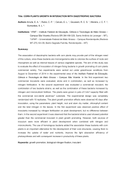
bargraph.CI(x.factor=FARM, group=VARIETY, response=YIELD, legend=T,
xlab="Location", ylab="Yield (kg/ha)", ylim=c(0,800),
cex.names=1, cex.lab=1,
x.leg=6, y.leg=700, cex.leg=1, leg.lab=c("Var A","Var B","Var C"),
col=grey.colors(3),
uc=T, lc=T, err.width=0.1, err.col="black", err.lty=1)

You can also do cross-hatching instead of colors. Try this for an old-fashioned look (add this to your
plot code, this will not run by itself):
col="black",

density=c(20,10,0), angle=c(45,-45,0),
By default, the error bars represent the standard error of the mean, but we can modify this with the
following additional customization. The first function will calculate the standard deviation instead, and
the second function will replace the default standard error with a 90% confidence interval (basically
the standard error multiplied by 1.96). We will soon learn the statistical theory behind this, so you can
program any confidence interval. Again, add this to your plot code (one line at the time). This will not
run by itself:
ci.fun=function(x) {c(mean(x)-sd(x), mean(x)+sd(x))}
ci.fun=function(x) {c(mean(x)-1.96*se(x), mean(x)+1.96*se(x))}

See if you can create this classic bar chart with standard deviations indicated only above the mean:
5.16. Line plots for factorial designs
If your treatments are in an ordered sequence, e.g. “Control”, “1 x Nitrogen”, “2 x Nitrogen”, “4 x
Nitrogen”, you may rather want to use a line graph. Multi-factor experiments can then be represented by
different lines (e.g. one line for “Farm 1” and one line for “Farm 2”, or whatever is your second treatment).
For illustration, I have generated a second dataset that is structured exactly like the farm dataset, but
here we don’t have a class variable as treatment as before (genetic varieties). Instead we have an
ordered sequence of nitrogen fertilizer levels. The most appropriate graph would be a line plot with
standard errors, which works exactly like the barplot.CI code above:

Import the dataset “fertilizer.csv”, which is downloadable from the website, run the code below, and
try to customize the plot to your liking (for more customization options run: ?lineplot.CI). See if
you can create the plot below the code.
library(sciplot)
lineplot.CI(x.factor=NITROGEN, group=FARM, response=YIELD,
col=c("black","gray"), pch=c(1,16), cex=1.5, lty=c(1,2),
xlab = "Nitrogen treatment (t/ha)", ylab="Yield (kg/ha)",
legend=T, x.leg=0.9, y.leg=27)
5.17. Dot charts
Dot charts can be used as an alternative to bar charts. They are generally easier to read when you have
many treatments, due to their high data-to-ink ratio. Also, they do not need to start with a 0 value to
convey the correct sense of the treatment effect (a problem with bar charts). Dot plots are the most highly
ranked graph type for perceptual accuracy (see Nature artcle in reading material: Fig 1c, right and Table
1, rank 1). However, bar charts are still a very familiar chart type and are widely used despite their
relatively low information density. Do use them if you only have a small number of treatment factors.

Unfortunately, the dot plot function does not automatically calculate summary statistics, so we have to
do that ourselves. Use Excel or PLYR to summarize the “fertilizer.csv” data:
library(plyr)
dat3 = ddply(dat,.(FARM,NITROGEN), summarise,
X=mean(YIELD), N=length(YIELD),
SE=sd(YIELD)/sqrt(length(YIELD)))
head(dat3)
attach(dat3)

Now let’s try some dot plots. We use the dotplot2 function of the package Hmisc, which you have to
install first. As with bar plots, there are different ways to group things:
graphics.off()
windows(width=4, height=4)
par (cex=1, family="sans", mar=c(5,5,5,5))
library(Hmisc)
dotchart2(X, FARM, groups=NITROGEN)
dotchart2(X, NITROGEN, groups=FARM)

As before, you can fully customize your graph with a number of familiar and graph-specific options
that you can look-up via ?dotchart2. Play with the options (bold) to remind yourself what they do:
dotchart2(X, NITROGEN, groups=FARM,
xlab="Yield (kg/h)", xlim=c(5,30),
cex.labels=1, cex.group.labels=1, groupfont=3,
width.factor=1.8, lty=2, lcolor="black",
pch=21, col="black", bg="gray", dotsize=1.5,
auxdata=N, auxtitle="N", sort.=F)

You can indicate standard errors by adding symbols (note that you have to include the “add and reset
parameter options for this to work properly):
dotchart2(X+SE, NITROGEN, groups=FARM, pch="|", add=T, reset.par=F)
dotchart2(X-SE, NITROGEN, groups=FARM, pch="|", add=T, reset.par=F)

Alternatively, you can use the same principle to add additional data. For illustration, I subset the dat3
dataset into Farm1 [1-3] and Farm2 [4-6] and add Farm2 data to the original Farm1 plot. See if you
can write additional lines to add and color the standard errors:
dotchart2(X[1:3], NITROGEN[1:3],
xlab="Yield (kg/h)", xlim=c(5,30),
width.factor=1.8, lty=2, lcolor="black",
pch=21, col="black", bg="red", dotsize=1.5)
dotchart2(X[4:6], NITROGEN[4:6], add=TRUE, reset.par=F,
pch=21, col="black", bg="blue", dotsize=1.5)
text(8,2.8,"Farm 1", col="red")
text(14,2.8,"Farm 2", col="blue")