Forecasting the yield curve with the arbitrage-free dynamic Nelson-Siegel model: Brazilian evidence Fabricio Tourrucôo12 João F. Caldeira3 Guilherme V. Moura4 André A. P. Santos5 Resumo Avaliamos se a imposição de uma restrição de não-arbitragem no modelo dinâmico de NelsonSiegel contribui para a obtenção de projeções mais acuradas da estrutura a termo. Para tal objetivo, conduzimos uma aplicação empírica para um amplo painel de contratos futuros de taxas de juro no Brasil e testamos as diferenças nos desempenhos das projeções para especificações alternativas incluindo: passeio aleatório, autoregressões (vetoriais) e o modelo dinâmico de Nelson-Siegel com fatores correlacionados e não-correlacionados. Mostramos empiricamente que o modelo livre-dearbitragem dinâmico de Nelson-Siegel supera todos os modelos alternativos quando horizontes de projeção mais longos são considerados. Palavras-chave: Curva de juros, modelo livre-de-arbitragem dinâmico de Nelson-Siegel, modelos de fatores dinâmicos, filtro de Kalman Abstract We assess the extent to which the imposition of a no-arbitrage restriction on the dynamic NelsonSiegel model helps obtaining more accurate forecasts of the term structure. For that purpose, we provide an empirical application based on a large panel of Brazilian interest rate future contracts and test for differences in forecasting performance among alternative benchmark specifications including the random walk, (vector) autoregressions, and the dynamic Nelson-Siegel model with both uncorrelated and correlated factors. We show empirically that the arbitrage-free Nelson-Siegel model is able to outperform all other benchmark models when longer forecasting horizons are taken into account. Keywords: Yield curve, arbitrage-free dynamic Nelson-Siegel model, Kalman filter dynamic factor models, JEL: E43, E47, G12, G17 Área 4 - Macroeconomia, Economia Monetária e Finanças. 1 2 3 4 5 Economia - Universidade Federal do Rio Grande do Sul – UFRGS Corresponding author e-mail: [email protected] Economia - Universidade Federal do Rio Grande do Sul - UFRGS Economia – Universidade Federal de Santa Catarina - UFSC Economia – Universidade Federal de Santa Catarina - UFSC Forecasting the yield curve with the arbitrage-free dynamic Nelson-Siegel model: Brazilian evidence Abstract We assess the extent to which the imposition of a no-arbitrage restriction on the dynamic NelsonSiegel model helps obtaining more accurate forecasts of the term structure. For that purpose, we provide an empirical application based on a large panel of Brazilian interest rate future contracts and test for differences in forecasting performance among alternative benchmark specifications including the random walk, (vector) autoregressions, and the dynamic Nelson-Siegel model with both uncorrelated and correlated factors. We show empirically that the arbitrage-free Nelson-Siegel model is able to outperform all other benchmark models when longer forecasting horizons are taken into account. Keywords: yield curve, arbitrage-free Nelson-Siegel model, dynamic factor models, Kalman filter 1. Introduction There has been growing interest in the ability to forecast the behavior of the term structure of interest rates. Such forecasts are of paramount importance for macroeconomists, financial economists and fixed income managers since bond portfolio optimization, pricing of financial assets and their derivatives, as well as risk management, rely heavily on interest rate forecasts. Moreover, these forecasts are widely used by financial institutions, regulators, and institutional investors to develop macroeconomic scenarios. One of the most popular approaches to forecast the yield curve is the the dynamic version of the Nelson & Siegel (1987) model proposed by Diebold & Li (2006) (hereafter DNS). Existing evidence suggests that these specifications are remarkably well suited both to fit the term structure and to forecast its movements (see, for example, Diebold & Rudebusch, 2013, and the references therein). Despite the large empirical evidence favorable to the DNS approach, one drawback is that it fails on an important theoretical dimension: it does not impose the restrictions necessary for riskless arbitrage opportunities, as shown in Björk & Christensen (1999). This drawback is relevant, since many financial applications that rely on interest rate modeling such as the pricing of interest-rate-linked assets require an arbitrage-free setting. This difficulty motivated Christensen et al. (2009) and Christensen et al. (2011) to develop an arbitrage-free version of the DNS model (hereafter AFNS), thus overcoming the theoretical weakness of the original model specification. The AFNS model of Christensen et al. (2009) and Christensen et al. (2011) has many appealing features. First, it preserves the desirable economic interpretation of the three-factor model of timevarying level, slope and curvature of the original DNS specification. Second, the AFNS ensures lack of arbitrage opportunities with a more parsimonious structure in comparison to general affine arbitrage-free models such as those considered in Duffie & Kan (1996) and Duffee (2002). More specifically, the way the AFNS achieves these desirable properties is by adding a yield-adjustment term to the original DNS specification which contains the necessary restrictions to ensure freedom of arbitrage. That being said, an immediate question that arises is the following: is the imposition of no-arbitrage helpful for forecasting purposes? This question is indeed very controversial. First, as we shall see in Preprint submitted to Elsevier July 19, 2014 Section 2.2, the yield-adjustment term of the AFNS model puts no restriction on the physical dynamics of yields. In other words, the imposition of no-arbitrage delivers yield-adjustment term that vary with maturity but are constant over time. This suggests that the inclusion of the yield-adjustment term is unlikely to provide forecasting gains. In particular, Duffee (2011) points out that imposition of no-arbitrage based on cross-section restrictions is irrelevant for forecasting.1 However, empirical work has found predictive gains from imposing no-arbitrage in a DNS framework. For instance, Gimeno & Marqués (2009) and Christensen et al. (2011) found that imposition of no-arbitrage leads to substantial forecast improvements. Diebold & Rudebusch (2013) point out that, despite its time constancy, the yield-adjustment term can act as a bias correction and thus produce forecast improvements.2 Clearly, additional empirical work is necessary in order to help clarify the gains (or lack of) coming from the imposition of no-arbitrage in the DNS class of models. In this paper we assess the extent to which the imposition of a no-arbitrage restriction on the DNS setting brings additional forecasting gains by providing an empirical evidence based on a large data set of constant-maturity future contracts of the Brazilian Inter Bank Deposit Future Contract (DI1) which is equivalent to a zero-coupon bond and is highly liquid (293 million contracts worth US$ 15 billion traded in 2010). The market for DI1 contracts is one of the most liquid interest rate markets in the world. Many banks, insurance companies, and investors use DI1 contracts as investment and hedging instruments. The data set considered in the paper contains daily observations of DI1 contracts traded on the Brazilian Mercantile and Futures Exchange (BM&F) with fixed maturities of 3, 6, 9, 12, 15, 18, 21, 24, 27, 30, 33, 36, 42, and 48 months. We use a rolling estimation to produce out-of-sample forecasts for 1-week, 1-month, 3-month, and 6-month ahead based on the DNS and AFNS models with both uncorrelated and correlated factors. Moreover, we consider three alternative classical benchmark specifications: the random walk (RW) model, which is taken as our baseline model, and the unrestricted first-order autoregressive (AR(1)) and vector-autoregressive (VAR(1)) models. We assess forecasting accuracy by means of the root mean squared forecast error (RMSFE) and the trace RMSFE (TRMSFE) considered in Hördahl et al. (2006) and de Pooter et al. (2010). Finally, we also test for the differences in forecasting performance using the test proposed in Giacomini & White (2006). Our empirical evidence suggests that when a short forecasting horizon is considered (e.g. 1-weekahead) the differences in forecasting performance among the candidate models is rather inconclusive since in very few instances the candidate models outperform the baseline RW model. However, when longer forecasting horizons are considered, the AFNS model with uncorrelated factors appears to deliver the most accurate forecasts in the vast majority of the cases. Therefore, the most important message from our empirical test is that the imposition of no-arbitrage is indeed helpful but only for longer (e.g. 3-month- and 6-month-ahead) forecasting horizons. These results corroborate the evidence reported in Christensen et al. (2011) for US Treasuries data, as they find that the AFNS model with indendent factors outperform the DNS specifications for the 6-month- and 12-month-ahead forecast horizons. The rest of the paper is organized as follows. Section 2 describes the DNS and AFNS specifications adopted in this paper. Section 3 discusses the implementation details and the empirical results. Finally, Section 5 concludes. 1 Coroneo et al. (2011) and Nyholm & Vidova-Koleva (2012) also found that the imposition of no-arbitrage adds little to forecasting accuracy. 2 Other authors such as Ang & Piazzesi (2003), Mönch (2008), Carriero (2011), Favero et al. (2012), among others, have also found that imposition of no-arbitrage leads to more accurate term structure forecasts. Moreover, Carriero & Giacomini (2011) show that the imposition of no-arbitrage restriction is important specially when an economic measure of accuracy is taken into account. 2 2. The Nelson-Siegel class of models Nelson & Siegel (1987) have shown that the term structure can be surprisingly well fitted at a particular point in time by a linear combination of three smooth functions. The Nelson-Siegel model of the yield curve is given by 1 − e−λτ 1 − e−λτ −λτ + τ (1) + β3 −e y(τ ) = β1 + β2 λτ λτ where y(τ ) is the zero-coupon yield with τ months to maturity, and β1 , β2 , and β3 can be interpreted as the level, slope, and curvature of the yield curve, respectively. The parameter λ determines the exponential decay of the β2 and β3 loadings. 2.1. Dynamic Nelson-Siegel model (DNS) Diebold & Li (2006) show that using the static Nelson-Siegel model as basis for a dynamic factor model generates highly accurate interest rate forecasts. The dynamic Nelson-Siegel model (DNS) is 1 − e−λτ 1 − e−λτ −λτ + X3t −e + t (τ ), (2) yt (τ ) = X1t + X2t λτ λτ where X1t , X2t , and X3t can be interpreted as the time-varying level, slope, and curvature factors. The DNS model can be interpreted as a dynamic factor model and written in state-space form. Consider the N × T matrix of observable yields (yt ), t = 1, . . . , T , where yt is the observation vector at time t, yt = (yit ) , i = 1, . . . , N . The DNS model can be represented in state-space form as yt = Γ + BXt + εt , εt ∼ N (0, Σ) , t = 1, . . . , T, Xt = µ + AXt−1 + ηt , ηt ∼ N (0, Ω) , t = 1, . . . , T, (3) (4) where B is the N × K matrix of factor loadings that depends on the decay parameter λ, Xt = (X1t , . . . , XKt )0 is a K-dimensional vector containing the coefficients, εt is the N × 1 vector of disturbances with Σ being its N × N diagonal covariance matrix. µ is a K × 1 vector of constants, A is the K × K transition matrix, and Ω is the conditional covariance matrix of disturbance vector ηt , which are independent of the residuals εt ∀t. Γ is a vector of constants, which is fixed to zero in the DNS specification but will be different from zero in the AFNS specification presented bellow. Equations (3) and (4) characterize a general Gaussian linear state-space model. Empirically, the DNS model is highly tractable and provides good fits. Theoretically, however, arbitrage opportunities cannot be prevented due to an unrestricted dynamic evolution of the yields. Indeed, as implied by Filipovic (1999), it is impossible to prevent arbitrage at bond prices in the resulting Nelson-Siegel yield curve. Christensen et al. (2011) showed how to remedy this theoretical weakness. 2.2. The dynamic arbitrage-free Nelson-Siegel model (AFNS) Aiming to overcome this theoretical weakness, but hoping to maintain the good properties of the DNS model, Christensen et al. (2011) have developed an arbitrage-free affine model in the spirit of Duffie & Kan (1996) which has the same factor loadings as the original DNS model. The resulting class of AFNS models involves considering the filtered probability space (Ω, F, (Ft ), Q) with filtration (Ft ) = {Ft : t ≤ 0} satisfying the usual conditions (see Williams, 1997). Q denotes the risk-neutral measure and we will denote the real world probability measure by P . The risk-neutral dynamic factors Xt are assumed to follow a Markov process defined on a set M ⊆ Rn that solves the stochastic differential equation (SDE) dXt = KQ (t) ΘQ (t) − Xt dt + Σ(t)D(Xt , t)dWtQ , (5) 3 where WQ is a standard Brownian Motion in Rn defined according to the filtration (Ft ). Furthermore, as in Duffie & Kan (1996) one assumes that the drifts, ΘQ : [0, T ] → Rn , dynamics, KQ : [0, T ] → Rn×n , and volatility, Σ : [0, T ] → Rn×n , are continuous functions. Finally, it is assumed that the mapping D : M × [0, T ] → Rn×n has a diagonal structure with entries p (6) [D]ii = γ i (t) + δ i (t)X1t + . . . + δ n (t)Xnt ∀i ∈ {1, . . . , n}, where γ i : [0, T ] → Rn and δ i : [0, T ] → Rn×n are continuous functions. In addition, Duffie & Kan (1996) assume the instantaneous risk-neutral rate is an affine function of the state variables rt = ρ0 (t) + ρ1 (t)0 Xt , (7) with continuous functions ρ0 : [0, T ] → R and ρ1 : [0, T ] → Rn . Under this affine formulation Duffie & Kan (1996) proved that a closed-form analytic expression for zero-coupon bond prices is attained as a linear function of the latent dynamic factors. This implies that the zero-coupon yield at time t for a bond with maturity T is given by: Z T 1 1 Q log E exp − [Γ(t, T ) + B(t, T )0 Xt ] (8) y(t, T ) = − ru du =− T −t T − t t where Γ(t, T ) and B(t, T ) satisfy the system of ordinary differential equations (ODEs) 0 P dΓ(t,T ) = ρ0 − B(t, T )0 KQ θQ − 12 ni=1 [Σ0 B(t, T )B(t, T )0 Σ]ii γ i , dt 0 P 0 dB(t,T ) = ρ1 + KQ B(t, T ) − 21 ni=1 [Σ0 B(t, T )B(t, T )0 Σ]ii (δ i ) , dt (9) with boundary conditions Γ(T, T ) = 0 and B(T, T ) = 0. Christensen et al. (2011) objective was to work under the generic affine latent factor dynamic structure proposed in(8) in order to rule out arbitrage opportunities. On the other hand, they had to impose additional restrictions on the ODE for B(t, T ) in (9) to ensure that it has solutions equal to the factor loadings of the DNS model: B 1 (t, T ) = − (T − t) , 1 − e−λ(T −t) , λ 1 − e−λ(T −t) + (T − t) e−λ(T −t) . B 3 (t, T ) = − λ B 2 (t, T ) = − This results in y(t, T ) = X1t + X2t 1 − e−λ(T −t) 1 − e−λ(T −t) Γ(t, T ) −λ(T −t) + X3t −e − , λ (T − t) λ (T − t) T −t (10) ) where DNS factor loadings are matched and the additional term − Γ(t,T is a correction to ensure the T −t model is arbitrage-free. Unlike the DNS models, which admit arbitrage, the AFNS models of Christensen et al. (2011) impose a particular structure on both the risk-neutral and real world latent factor dynamic processes. Christensen et al. (2011), following Singleton (2006), argue that not all parameters in the specification (5-7) can be identified so that identifying restrictions must be imposed under the Q measure. Specifically, 4 the mean ΘQ = 0, the volatility matrix Σ is triangular, σ11 0 0 Σ = σ21 σ22 0 , σ31 σ32 σ33 ρ0 = 0, ρ1 = (1, 1, 0)0 , δ = 0, γ = (1, . . . , 1)0 , and the state-variable reversion rate 0 0 0 K Q = 0 λ −λ . 0 0 λ ) is of the form Under those restrictions, the yield adjustment term − Γ(t,T T −t 3 Γ(t, T ) 1 1 X = T −t 2 T − t i=1 Z T [Σ0 B(s, T )B(s, T )0 Σ]ii ds, (11) t the instantaneous risk-neutral rate is given by rt = X1t + X2t , and the latent state variables Xt = (X1t , X2t , X3t ) are described by the system of SDEs under the risk-neutral measure Q dW1tQ dX1t X1t dX2t = −K Q X2t dt + Σ dW2tQ , λ > 0. dX3t X3t dW3tQ This completes the specification of the AFNS model under the risk-neutral measure. 2.2.1. Independent and correlated AFNS models We consider two versions of the DNS model and investigate the effect of the arbitrage-free restriction on their corresponding AFNS versions. The first is the uncorrelated-factor DNS model which is specified in terms of a diagonal transition matrix in (4). The correlated-factor DNS model has a full transition matrix instead. In both DNS models the measurement equation is the same. The corresponding AFNS models are formulated in continuous time and the relation between the dynamics under measures Q and P is given by a change of measure that preserves the affine dynamic structure (see Christensen et al. (2011) for full details). This is a very convenient property since it guarantees that identical (P-measure) models can be estimated. Using the solution already presented in (10), yields must be related to the state variables by yt = Γ + BXt + εt . (12) Comparing equations (2) and (10), we notice that the matrix B is identical for DNS and AFNS models. The only difference is the added vector Γ containing the yield-adjustment terms in the AFNS models. Since the AFNS is a continuous model, the dynamics is discretized to allow comparison with the discretetime DNS models. The estimation is outlined in the next section. For the uncorrelated-factor AFNS model the dynamics of the state variables under the P-measure is P P dX1t κ11 0 0 θ1 X1t σ11 0 0 dW1tP dX2t = 0 κP22 0 θ2P − X2t dt + 0 σ22 0 dW2tP . (13) dX3t 0 0 κP33 θ3P X3t 0 0 σ33 dW3tP 5 In the correlated-factor AFNS model, the three shocks may be correlated, and there may be full interaction among the factors as they adjust to the steady state P P θ1 X1t dX1t σ11 0 0 κ11 κP12 κP13 dW1tP dX2t = κP21 κP22 κP23 θ2P − X2t dt + σ21 σ22 0 dW2tP . (14) κP31 κP32 κP33 θ3P X3t dX3t σ31 σ32 σ33 dW3tP This is the most flexible version of the AFNS models, where all parameters are identified. From these specifications we see the striking resemblance between DNS and AFNS models. 2.2.2. An exact expression for the covariance of the continuous-time AFNS model In this paper, the models are estimated using a maximum likelihood estimation method based on the Kalman filter discussed in Section 3. The AFNS model can be formulated in a state-space form as follows. Departing from the continuous-time formulation of the AFNS model, the conditional mean vector and the conditional covariance matrix are EP [XT |Ft ] = I − exp(−KP ∆t) ΘP + exp(−KP ∆t)Xt (15) Z ∆t exp(−KP s)ΣΣ0 exp(−(KP )0 s)ds (16) VP [XT |Ft ] = 0 To estimate the AFNS models proposed by Christensen et al. (2011) we must compute the conditional covariance matrix Z ∆t exp(−KP s)ΣΣ0 exp(−(KP )0 s)ds VP [Xt | Ft−1 ] = (17) 0 of discrete observations. Since the estimation is an intense computational process, we need to provide fast intermediate calculations. One approach is to approximate the integral and the matrix exponential. Another approach uses the diagonalization of KP to calculate the integral exactly. Due to the reduced size of the matrix KP , the latter is significantly faster than the former. The AFNS state transition is Xt = I − exp −KP ∆t ΘP + exp −KP ∆t Xt−1 + ηt , where ∆t is the time between the observations at t and t − 1, with measurement equation yt = Γ + BXt + εt , and error structure ηt 0 Q 0 ∼N , , εt 0 0 H where H is diagonal, Q = VP [Xt | Ft−1 ] and the transition and measurement errors are assumed orthogonal to the initial state. The computation of Q is straightforward if we use the diagonalization of KP KP = V ΛV −1 , (18) where V contains the eigenvectors of KP , and Λ is a diagonal matrix containing the eigenvalues (λi ) of KP . We refer the reader to Lang (1987) and Golub & Van Loan (1996) for details on linear algebra theory and on the computational aspects of linear algebra, respectively. 6 Substituting (18) in (17), using exp(−KP s) = V exp(−Λs)V −1 , and similarly exp(− KP we obtain Z Q=V T ∆t s) = V −1 T exp(−Λs)V T , exp(−Λs)Ω exp(−Λs)ds V T , 0 T −1 T where Ω = (ωij )n×n = V −1 ΣΣ (V ) . Since the exponential of a diagonal matrix with entries −λi s is a diagonal matrix with entries e−λi s , each term of the matrix under the integral is (ωij e−(λi +λj )s )n×n . Integration yields an expression which only involves matrix multiplications ωij −(λi +λj )∆t V T. (19) 1−e Q=V λi + λj n×n Stationarity of the system under the P-measure is ensured if the real parts of all eigenvalues of KP are positive, and this condition is imposed in all estimations. For this reason, we can start the Kalman filter at the unconditional mean, X0 = ΘP , and covariance matrix, Σ0 . In particular, the unconditional R∞ variance Σ0 = 0 exp(−KP s)ΣΣ0 exp(−(KP )0 s)ds used in the initialization of the filter is easily obtained from the above expression. Assuming KP has eigenvalues with positive real parts, the integral converges to ωij Σ0 = V V T. (20) λi + λj n×n 3. Data and estimation framework In this section we describe the estimation method and present the data set used in the empirical analysis. Specifically, we estimate the three-factor dynamic Nelson-Siegel model of Diebold & Li (2006) and the arbitrage-free Nelson and Siegel model developed by Christensen et al. (2011) via Maximum Likelihood. Benchmark models used include the Random Walk forecast (RW), linear autoregressive (AR) and vector autoregressive models (VAR). 3.1. Estimation of the DNS and AFNS models Given the state space formulation of the dynamic factor model presented in (3) and (4), the Kalman filter can be used to obtain the likelihood function via the prediction error decomposition, as well as filtered estimates of the states and of their covariance matrices. However, the computational burden associated with the Kalman filter recursions depends crucially on the dimension of both the state and observation vectors. Moreover, in yield curve models the dimension of the observation vector (N × 1) is often much larger than that of the state vector (K × 1). In these circumstances, Jungbacker & Koopman (2014) have shown that significant computational gains can be achieved by a simple transformation. First, define the N × N and the K × N matrices: L J J= , J L = CΛ(λ)0 Σ−1 , JH 7 respectively, where C can be any K × K invertible matrix, and J H is chosen to guarantee that J is full −1 rank. Selecting C = (Λ(λ)0 Σ−1 Λ(λ)) implies: L L L L J (yt − Γ) yt ft A εt A εt C 0 J(yt −Γ) = = = + , ∼ N 0, . J H (yt − Γ) ytH 0 AH εt AH εt 0 ΣH The law of motion of the factors in (4) is not affected by the transformation. Note that ytH is neither dependent on ft , nor correlated with ytL and, therefore, does not need to be considered for the estimation of the factors. This implies that the Kalman filter only needs to be applied to the low dimensional subvector ytL for signal extraction, generating large computational gains when N >> K (see Table 1 of Jungbacker & Koopman, 2014). Denote l(y) the log-likelihood function of the untransformed model in (3) and (4), where y = 0 (y1 , . . . , yT0 )0 . Evaluation of l(y) can also take advantage of the transformations presented above. Jungbacker & Koopman (2014) show that the log-likelihood of the untransformed model can be represented as T |Σ| 1 X 0 −1 T − e Σ et , l(y) = c + l(y ) − log 2 |C| 2 t=1 t L (21) where c is a constant independent of both y and the parameters, l y L is the log-likelihood function of the reduced system, and et = yt − Γ − Λ(λ)ft . Note that computation of matrix J H is not required at any point, as proved in Lemma 2 of Jungbacker & Koopman (2014). 3.2. Data The analyzed data set consists of Brazilian Interbank Deposit Futures Contract (DI1)3 . DI1 market is one of the largest fixed-income markets among emerging economies. We use DI1 daily closing yields of available contracts. Since not all maturities are observed on a daily basis, we interpolate the available data using cubic splines to produce yield curves with fixed maturities. The chosen fixed maturities are: 3, 6, 9, 12, 15, 18, 21, 24, 27, 30, 33, 36, 42, and 48 months. The DI1 contract with maturity τ is a zero-coupon future contract in which the underlying asset is the DI interest rate accrued on a daily basis, capitalized between trading days t and τ 4 The value of contract is set by its value at maturity, R$100, 000.00, discounted according to the accrued interest rate negotiated between the seller and the buyer. In 2010 the DI1 market traded a total of 293 million contracts corresponding to US$ 15 billion. The DI1 contract is very similar to the zero-coupon bond, except for the daily payment of margin adjustments. The data set contains liquid maturities from 3 BM&FBOVESPA is the entity that offers the DI1 contract and determines the number of maturities with authorized contracts. 4 The DI rate is the average daily rate of Brazilian Interbank Deposits (borrowing/lending), calculated by the Clearinghouse for Custody and Settlements (CETIP) for all business days. The DI rate, which is published on a daily basis, is expressed in annually compounded terms, based on 252 business days. When buying a DI1 contract at the DI ? rate at time t and keeping it until maturity τ , the gain or loss is given by: ! Qζ(t,τ ) 1 252 (1 + y ) i i=1 100.000 −1 , ζ(t,τ ) (1 + DI ∗ ) 252 where yi denotes the DI rate, (i − 1) days after the trading day. The function ζ(t, τ ) represents the number of working days between t and τ . 8 January 2006 to December 2012, with a total of T = 1488 daily observations. The data source is the Brazilian Mercantile and Futures Exchange (BM&F). Table 1 reports descriptive statistics for the Brazilian interest rate yield curve based on the DI1 market. For each time series we report the mean, standard deviation, minimum, maximum and the lag1 sample autocorrelation. The summary statistics confirm some common stylized facts to yield curve data: the sample average curve is upward sloping and concave, volatility is decreasing with maturity, and autocorrelations are very high. Table 1: Descriptive statistics for the term structure of interest rates The Table reports summary statistics for DI1 yields over the sample period January 2007 - December 2012 (1488 daily observations). We examine daily data, constructed using cubic splines. Maturity is measured in months. We show, for each maturity, mean, standard deviation, minimum, maximum and and a selection of autocorrelation (Acf, ρb(1), ρb(5), and ρb(21), respectively) and partial autocorrelation (Pacf, α b(2) and α b(5)) coefficients. Maturity τ Mean Std Dev Min Max Skew Kurt ρb(1) Acf ρb(5) ρb(21) α b(2) Pacf α b(5) Month 1 3 6 9 12 15 18 21 24 27 30 36 42 48 10.66 10.66 10.73 10.85 11.00 11.16 11.31 11.42 11.52 11.60 11.66 11.75 11.83 11.89 1.75 1.79 1.86 1.90 1.92 1.92 1.88 1.85 1.81 1.77 1.74 1.66 1.59 1.56 6.97 7.02 6.91 6.86 6.87 6.90 7.00 7.14 7.32 7.49 7.65 7.91 8.13 8.29 14.13 14.52 15.32 16.04 16.40 16.91 17.12 17.26 17.44 17.62 17.78 17.83 17.93 18.00 -0.337 -0.286 -0.201 -0.132 -0.091 -0.053 -0.046 -0.042 -0.032 -0.004 0.028 0.080 0.104 0.181 2.219 2.296 2.472 2.650 2.784 2.907 3.002 3.118 3.243 3.375 3.504 3.731 3.937 4.156 0.998 0.998 0.998 0.998 0.997 0.997 0.997 0.997 0.996 0.996 0.996 0.995 0.995 0.995 0.987 0.989 0.989 0.988 0.987 0.985 0.984 0.983 0.982 0.981 0.980 0.978 0.976 0.975 0.936 0.940 0.939 0.934 0.929 0.923 0.917 0.912 0.907 0.901 0.895 0.887 0.880 0.873 -0.016 -0.017 -0.012 0.004 0.019 0.024 0.020 0.023 0.020 0.015 0.010 0.015 0.017 0.018 -0.012 -0.025 -0.023 -0.010 0.000 0.003 0.002 -0.002 -0.001 -0.002 -0.006 -0.013 -0.006 -0.011 Level Slope Curvature 12.41 -1.92 -1.00 1.42 1.95 3.94 9.34 -6.37 -9.48 18.99 2.84 8.60 0.673 -0.267 0.120 5.185 2.814 2.192 0.992 0.995 0.997 0.957 0.974 0.978 0.800 0.866 0.903 -0.064 -0.039 -0.160 -0.014 -0.036 -0.011 Figure 1 displays a three-dimensional plot of the data set and illustrates how yield levels and spreads vary substantially throughout the sample. The plot also suggests the presence of an underlying factor structure. Although the yield series vary substantially over time for each maturity, a strong common pattern in the 14 series is apparent for most of them: the yield curve is an upward-sloping function of maturity. For example, the last year of the sample is characterized by rising interest rates, especially for the shorter maturities, which respond faster to the contractionary monetary policy implemented by the Brazilian Central Bank in the first half of 2010. It is clear from Figure 1 that not only the term structure level fluctuates over time but also its slope and curvature. The curve takes on various forms ranging from nearly flat to (inverted) S-type shapes. 4. Empirical analysis In this section we investigate whether the in-sample superiority of the flexible correlated-factor model carries over to out-of-sample forecast accuracy. Estimates for the vector of factor means, µ, and the λ parameter are very similar for both the uncorrelated and correlated DNS models, as can be seen on Table 2 and on Table 3. The mean of 9 Figure 1: Evolution of the yield curve Evolution of the term structure of interest rates (based on DI1 contracts) for the 2006:01-2012:12 period. The sample consists of the daily yields for maturities of 1, 3, 4, 6, 9, 12, 15, 18, 24, 27, 30, 36, 42, and 48 months. the level, slope, and curvature factors are 12.56%, −2.21%, and −0.84% in the uncorrelated model, respectively, and 12.03%, −3.44%, and 0.80% for the correlated model, respectively. All figures are in accordance with observable empirical yield curves. The transition matrices reveal that the factors are highly persistent, being well above 0.9 for both estimated DNS models. The correlated transition matrix shows only very mild correlation. Table 2: Estimates for the uncorrelated DNS model Estimated uncorrelated DNS model. All numbers are in decimals. State transition matrix A is enforced to be diagonal. Corresponding error matrix Q is enforced to be diagonal and positive semi-definite (using Cholesky factorization Q = qq 0 ). Vector µ contains the level, slope, and curvature factor means. The estimated λ is 1.4377, where time measured in years. A matrix A.,1 A.,2 A.,3 Means µ q.,1 Q matrix q.,2 q.,3 A1,. 0.9873 0 0 0.1256 q1,. 4.61 × 10⁻⁶ 0 0 A2,. 0 0.9496 0 −0.0221 q2,. 0 6.00 × 10⁻⁶ 0 A3,. 0 0 0.9809 −0.0084 q3,. 0 0 5.30 × 10⁻⁵ Variances of the state variables are similar across the uncorrelated and correlated DNS models, except for the variance of shocks to the curvature parameter. The covariance estimates obtained in the correlated-factor DNS model translate into a correlation of −0.795 for innovations to the level and slope factor, a correlation of 0.330 for innovations to the level and curvature factor, and a correlation of −0.234 for innovations to the slope and curvature factor. These correlations allow interesting geometrical interpretations: when the yield curve level increases, it gets steeper, and more concave. The slope effect is higher than the curvature effect, and the correlation between slope and curvature reinforces slightly the concavity effect. 10 Table 3: Estimates for the correlated DNS model Estimated correlated DNS model. All numbers are in decimals. Corresponding error matrix Q are enforced to be positive semi-definite (using Cholesky factorization Q = qq 0 ). Vector µ contains the level, slope, and curvature factor means. The estimated λ is 1.3272, where time is measured in years. A.,1 A matrix A.,2 A.,3 Means µ Q matrix q.,2 q.,1 q.,3 A1,. 0.9898 0.0318 −0.0063 0.1203 q1,. 4.84 × 10⁻⁶ 0 0 A2,. 0.0394 0.9945 0.0392 −0.0344 q2,. −4.62 × 10⁻⁶ 6.97 × 10⁻⁶ 0 A3,. −0.0032 −0.0610 0.9462 0.0080 q3,. 6.38 × 10⁻⁶ −5.43 × 10⁻⁶ 7.71 × 10⁻⁵ Estimates of the level factor mean are noticeably higher in AFNS models when compared to both DNS formulations, while slope and curvature are of similar magnitude, as can be seen on Table 4 and on Table 5. λ is slightly higher for correlated DNS and AFNS models. The higher λ makes the slope and curvature factor loadings decay to zero faster. Table 4: Estimates for the uncorrelated AFNS model Estimated uncorrelated AFNS model. Estimated state transition matrix K is enforced to be diagonal. Corresponding error matrix Σ is enforced to be diagonal and positive semi-definite (using Cholesky factorization). θ is the vector of factor means (level, slope, and curvature). The associated estimated λ is 1.4039, where time is measured in years. KP matrix κP.,2 κP.,1 κP.,3 Mean θP Σ.,1 Σ matrix Σ.,2 Σ.,3 κP1,. 3.1873 0 0 0.1294 Σ1,. 0.0334 0 0 κP2,. 0 1.1755 0 −0.0233 Σ2,. 0 0.0315 0 κP3,. 0 0 1.1027 −0.0258 Σ3,. 0 0 0.0572 While λ and θ are directly comparable to the decay parameter and vector of factor means in the DNS model, the state transition and covariance matrices are modeled continuously and need to be converted to be comparable. The continuous state transition matrix (K) and volatility matrix (Σ) are converted into one-day (the time between observations) conditional matrices. Given the mean-reversion P 1 rate matrix K, its daily counterpart can be computed as exp −K 252 . For the volatility matrix Σ, its discrete version is computed as AFNS Q Z = 1 252 exp(−KP s)ΣΣ0 exp(−(KP )0 s)ds, 0 1 which is based on equation (17) with ∆t = 252 . Results are presented on Table 6. The same conversion procedure is used in the correlated AFNS model to ensure comparison (see Table 7). Results are similar to the ones reported for the correlated-factor DNS model. The curvature factor becomes slightly more persistent in the AFNS model, while the level becomes slightly less persistent. The yield adjustment term is the key difference in the measurement update between the AFNS and 11 Table 5: Estimates for the correlated AFNS model Estimated correlated AFNS model. Estimated state transition matrix K is fully flexible. Corresponding error matrix Σ is enforced to be lower-triangular and positive semi-definite (using Cholesky factorization). θ is the vector of factor means (level, slope, and curvature). The associated estimated λ is 1.3419, where time is measured in years. κP.,1 KP matrix κP.,2 κP.,3 Mean θP Σ.,1 Σ matrix Σ.,2 Σ.,3 κP1,. 3.1408 −0.0604 0.0254 0.1418 Σ1,. 0.0401 0 0 κP2,. −2.6261 1.2257 −1.4691 −0.0344 Σ2,. −0.0406 0.0220 0 κP3,. −0.0412 1.8640 1.9921 −0.0192 Σ3,. −0.0355 −0.0926 0.0684 Table 6: One-day parameters for uncorrelated AFNS model K and Σ converted into daily estimates to ensure comparison with A and Q. One-day mean reversion matrix 0.9874 0 One-day volatility matrix 4.38 × 10⁻⁶ 0 0 0 0.9953 0 0 3.93 × 0 0 0.9956 0 0 0 10−6 0 5.29 × 10⁻⁵ DNS models. The adjustment terms for both AFNS models are shown in Figure 2. The yield adjustment term increases the flexibility of the curve fitting, especially at longer maturities. Furthermore the offdiagonal elements of matrix Σ are heavily influenced by the shape of the adjustment terms. The shape of the almost linear adjustment term is not surprising for the uncorrelated AFNS model since all off-diagonals in Σ are forced to be zero, meaning there are no negative covariances to offset the decreasing function of maturity. However, the more flexible correlated AFNS model can have covariances that change the shape of the adjustment term. Nevertheless, due to the low off-diagonal for the correlated covariance matrix, the effect on the shape of the adjustment term is small. In fact, the very low yield adjustment term in both AFNS cases (highlighted by the considerably lower variances than the DNS models) implies that very little adjustment is needed to make the DNS model arbitrage-free. To further investigate in-sample model performance, residual means for each maturity together with root-mean-square-errors (RMSE) are presented on Table 8. Based on Table 8 alone, it is very hard to rank models, but it does indicate that the simpler DNS models outperform the AFNS counterpart at least in-sample. The lowest RMSEs of 12 out of 13 maturities belong to the DNS class, out of which, eight belong to the uncorrelated DNS model. The absence of arbitrage restrictions do not seem to improve in-sample fit. Given the relatively small yield adjustment terms presented in Figure 2, the lack of improvement in fit is not very surprising. 4.1. Out-of-sample analysis The forecasting test is performed in pseudo-real time, i.e., we never use information which is not available at the time the forecast is made. We use a rolling estimation window of 500 daily observations 12 Table 7: One-day parameters for correlated AFNS model K and Σ converted into daily estimates to ensure comparison with A and Q. One-day mean reversion matrix One-day volatility matrix 0.9876 0.0002 −0.0001 4.38 × 10⁻⁶ −6.39 × 10⁻⁶ −5.57 × 10⁻⁶ 0.0103 0.9951 0.0058 −6.39 × 10⁻⁶ 8.34 × 10⁻⁶ −2.24 × 10⁻⁶ −0.0557 −0.0224 0.9921 −5.57 × 10⁻⁶ −2.24 × 10⁻⁶ 5.72 × 10⁻⁵ Figure 2: Yield adjustment term for the AFNS models ) Yield adjustment term, −A(τ τ , in basis points. Maturity is measured in years. The solution is provided in Christensen et al. (2011). 0.000 indep. AFNS yield adj. corr. AFNS yield adj. Yield Adjustment Term −0.001 −0.002 −0.003 −0.004 −0.005 −0.006 −0.007 0.5 1 1.5 2 2.5 3 3.5 4 Maturity in Months (2 years). We produce forecasts for 1-week, 1-month, 3-months, and 6-months ahead. The choice of a rolling scheme is suggested by two reasons: first, it is a natural way to avoid problems of instability, see e.g. Pesaran et al. (2011). Second, having a fixed number of observations used to compute the forecasts, the resulting time series of forecast errors can be tested for accuracy by the Giacomini & White (2006) test. It is worth noting that we use iterated forecasts instead of direct forecasts for the multi-period ahead predictions. Marcellino et al. (2005) argue that iterated forecasts are more efficient when the model is correctly specified. In order to evaluate out-of-sample forecasts, we compute popular error metrics. Given a sample of M out-of-sample forecasts for an h-period-ahead forecast horizon, we compute the root mean squared forecast error (RMSFE) for maturity τi and for model m as follows: v u M u 1 X 2 t RMSFEm (τi ) = ŷt+h|t,m (τi ) − yt+h (τi ) (22) M t=1 13 Table 8: Descriptive statistics of in-sample fit The means and the root mean squared errors for 13 different maturities. All numbers are measured in basis points. DNS Maturity Months τ indep-factor Mean RMSE dep-factor Mean RMSE AFNS indep-factor Mean RMSE dep-factor Mean RMSE 3 -7.05 19.54 -4.06 18.00 -0.02 0.03 -14.64 24.28 6 -0.01 0.01 1.07 1.07 8.38 14.77 -0.03 0.02 9 3.18 6.71 3.56 6.74 11.01 17.28 6.52 9.50 12 3.06 6.65 3.33 6.70 9.35 14.01 7.21 10.63 15 1.11 4.39 1.53 4.54 5.49 8.83 4.68 7.97 18 -0.29 2.31 0.36 2.32 2.19 3.94 2.07 4.09 21 -0.94 2.41 -0.06 2.19 -0.16 0.91 0.04 0.07 24 -0.92 3.07 0.15 2.95 -1.49 2.79 -1.3 3.13 27 -0.56 3.22 0.68 3.24 -2.05 3.75 -1.98 4.53 30 0.66 3.39 2.02 3.85 -1.30 3.57 -1.43 4.49 36 1.94 3.39 3.42 4.35 0.42 2.37 -0.21 3.55 42 0.43 2.54 1.88 3.04 1.13 2.74 0.00 0.00 48 -2.37 5.40 -1.09 5.20 2.22 5.36 0.65 4.38 where yt+h (τi ) is the yield for the maturity τi observed at time t + h, and ŷt+h|t,m (τi ) is the corresponding forecasting made at time t. Following Hördahl et al. (2006) and de Pooter et al. (2010), we also summarize the forecasting performance of each model by computing the trace root mean squared forecast error (TRMSFE). For each forecast horizon, we compute the trace of the covariance matrix of the forecast errors across all N maturities. Hence, lower TRMSFE indicate more accurate forecasts. The TRMSFE can be computed as v u N X M u1 1 X 2 ŷt+h|t (τi ) − yt+h (τi ) (23) TRMSFEm (τi ) = t N M i=1 t=1 Finally, in order to assess the statistical significance of these forecasting differences, we use the test proposed by Giacomini & White (2006). The Giacomini & White (2006) (GW) test is a conditional forecasting ability test constructed under the assumption that forecasts are generated using a moving data window. This is a test of equal forecasting accuracy and as such can handle forecasts based on both nested and non-nested models, regardless from the estimation procedures used in the derivation of the forecasts. The test is based on the loss differential dm,t = (erw,t )2 − (em,t )2 , where emt is the forecast error of model m at time t. We assume that the loss function is quadratic but it can be replaced by other loss functions depending on the forecast goal. The null hypothesis of equal forecasting accuracy can be written as H0 : E [dm,t+h |δm,t ] = 0, (24) where δm,t is a p × 1 vector of test functions or instruments and h is the forecast horizon. If a constant 14 is used as instrument, the test can be interpreted as an unconditional test of equal forecasting accuracy. The GW test statistic GWm,t can be computed as the Wald statistic: GWm,n = n n−1 n−h X !0 δm,t dm,t+h n−1 Ω̂−1 n n−h X ! δm,t dm,t+h d −→ χ2dim(δ) (25) t=ω+1 t=ω+1 where Ω̂n is a consistent HAC estimator for the asymptotic variance of δm,t dm,t+h , and n = (T − ω) the number of out-of-sample observations. Under the null hypothesis given in (24), the test statistic GWi,t is asymptotically distributed as χ2p . The asterisks on Tables 9 and 10 denote significant differences in out-of-sample model performance relative to RW at the 5, and 10 percent levels. Tables 9 and 10 report the RMSFE and TRMSFE for each of the forecasting models and for each of the forecasting horizons. The first column in each panel of each Table reports the value of RMSFE and TRMSFE (expressed in basis points) for the random walk model (RW), while all other columns report statistics relative to the RW. The following model abbreviations are used on Tables 9 and 10: AR(1) for the first-order univariate autoregressive model, VAR(1) for the first-order vector autoregressive model, DNSAR for the dynamic Nelson-Siegel model with a (V)AR specification for the factors, and AFNS for the dynamic Arbitrage-Free Nelson Siegel model with a (V)AR specification for the factors. First, the RW confirms to be a very competitive benchmark in forecasting the term structure of bond yields, especially at short horizons. For each forecasting horizon considered, we highlight the most accurate model, in terms of RMSFE, for each of the 13 maturities analyzed. Bold values indicate relative differences below one, which means that a particular model outperforms the random walk. Stars denote rejection of the null of equal forecasting ability according to the GW test at 5% and 1% level. Comparing correlated to uncorrelated factor models, we notice that the most parsimonious specification performs better for AFNS but not for DNS. For the latter, VAR parameterization of the factor dynamics achieves better forecasting results. As pointed out, the DNS model outperformed the AFNS model in-sample in terms of RMSE. When analyzing out-of-sample performance, we observe that the DNS model is superior to the other competitors in almost all maturities when short-horizon forecasts are considered (1-week and 1-month). These results are in line with Duffee (2002), who conclude that affine term structure models can have very poor performance out-of-sample. However, for longer forecasting horizons (3 to 6-months ahead), the AFNS model outperforms all competitors for all maturities. Nevertheless, DNS still outperforms RW, showing its good forecasting capabilities. What is striking here is that the arbitrage-free restrictions seem to improve a lot the long run forecasts, since most of the differences in RMSFE are statistically significant. Moreover, the uncorrelated AFNS version is the best performing model for almost all maturities, except for short maturities, when it is beaten by the correlated AFNS model. For the 1-week ahead forecasts, the best performing model overall in terms of T-RMSFE is the RW model. However, for 1-month ahead forecasts the correlated factors DNS model performs best, while for the longer forecast horizons of 3- and 6-months ahead the best performing model in terms of T-RMSFE was the AFNS, evidencing the forecast benefits of imposing the arbitrage-free restriction. 15 Table 9: Out-of-sample Yield Forecasts : [T] RMSFEs Note: This table summarizes Relative Mean Squared Forecast Errors and Trace Root Mean Squared Forecast Error (TRMPSE) relative to the Random Walk obtained by using each of the competing models, for the horizons 1-week, 1-, 3-, and 6-month-ahead. The first column in the table reports the value of (T) RMSFE (expressed in basis points) for the Random Walk model (RW), while all other columns report statistics relative to the RW. The following model abbreviations are used in the table: RW stands for the Random Walk, (V)AR for the first-order (Vector) Autoregressive Model, DNS for the one-step dynamic Nelson-Siegel model with a (V)AR specification for the factors, AFNS refers to the one-step Arbitrage-Free Nelson Siegel model with a (V)AR specification for the factors. Numbers smaller than one (shown in bold) indicate that models outperform the random walk, whereas numbers larger than one indicate underperformance. The gray box indicate outperformance in the maturity. The stars on the right of the cell entries signal the level at which the Giacomini & White (2006) test rejects the null of equal forecasting accuracy (∗ and ∗∗ mean respectively rejection at 1% and 5% level). 1-week-ahead forecasts 1-month-ahead forecasts Maturity 16 RW AR(1) VAR(1) DNSAR DNSVAR AFNSAR AFNSVAR RW AR(1) VAR(1) DNSAR DNSVAR AFNSAR AFNSVAR 3 6 9 12 15 18 21 24 27 30 36 42 48 0.120 0.141 0.154 0.164 0.174 0.181 0.183 0.184 0.187 0.188 0.188 0.189 0.192 0.986 0.994 0.999 1.003 1.006 1.008 1.011 1.013 1.013 1.014 1.016 1.018 1.019 0.764∗ 0.928 1.015 1.062 1.105 1.130 1.152 1.162 1.159 1.160 1.162 1.169 1.166 0.990∗∗ 1.384 1.430 1.269 1.104 1.023 1.005 0.993 0.988 0.993 1.004 1.010 1.044 2.211 0.961 1.120 1.152 1.090 1.045 1.045 1.067 1.083 1.060 1.035 1.040 1.058 1.792 1.149 1.222 1.194 1.126 1.083 1.081 1.079 1.074 1.080 1.085 1.053 1.042 1.494 0.858∗ 1.001 1.033 1.031 1.033 1.052 1.032 1.030 1.053 1.072 1.039 1.054 0.409 0.430 0.442 0.445 0.455 0.459 0.458 0.453 0.453 0.452 0.437 0.420 0.417 0.994 0.997 1.001 1.006 1.012 1.017 1.023 1.029 1.031 1.036 1.045 1.056 1.061 0.573∗ 0.749∗∗ 0.858 0.963 1.040 1.101 1.139 1.162 1.158 1.159 1.198 1.230 1.230 0.995∗∗ 1.008 1.017 1.021 1.011 1.006 1.002 0.990 0.977∗∗ 0.980∗ 1.005 1.009 1.011 1.113 0.960∗∗ 0.955 0.964 0.958 0.954 0.953 0.948 0.942 0.944 0.969 0.978 0.983 1.192 1.162 1.164 1.166 1.146 1.130 1.128 1.128 1.120 1.119 1.134 1.125 1.092 0.576∗ 0.693∗ 0.845 0.956 1.021 1.064 1.101 1.104 1.100 1.109 1.129 1.107 1.077 T-RMSFE 0.170 1.010 1.116 1.086 1.127 1.132 1.052 0.440 1.024 1.065 1.002 0.969 1.139 1.011 Table 10: Out-of-sample Yield Forecasts : [T] RMSFEs Note: This table summarizes Relative Mean Squared Forecast Errors and Trace Root Mean Squared Forecast Error (TRMPSE) relative to the Random Walk obtained by using each of the competing models, for the horizons 1-week, 1-, 3-, and 6-month-ahead. The first column in the table reports the value of (T) RMSFE (expressed in basis points) for the Random Walk model (RW), while all other columns report statistics relative to the RW. The following model abbreviations are used in the table: RW stands for the Random Walk, (V)AR for the first-order (Vector) Autoregressive Model, DNS for the one-step dynamic Nelson-Siegel model with a (V)AR specification for the factors, AFNS refers to the one-step Arbitrage-Free Nelson Siegel model with a (V)AR specification for the factors. Numbers smaller than one (shown in bold) indicate that models outperform the random walk, whereas numbers larger than one indicate underperformance. The gray box indicate outperformance in the maturity. The stars on the right of the cell entries signal the level at which the Giacomini & White (2006) test rejects the null of equal forecasting accuracy (∗ and ∗∗ mean respectively rejection at 1% and 5% level). 3-month-ahead forecasts 6-month-ahead forecasts Maturity 17 RW AR(1) VAR(1) DNSAR DNSVAR AFNSAR AFNSVAR RW AR(1) VAR(1) DNSAR DNSVAR AFNSAR AFNSVAR 3 6 9 12 15 18 21 24 27 30 36 42 48 1.134 1.192 1.234 1.248 1.252 1.236 1.221 1.200 1.196 1.190 1.154 1.106 1.084 1.077 1.085 1.078 1.071 1.067 1.066 1.071 1.085 1.105 1.124 1.144 1.176 1.205 0.727∗ 0.950∗∗ 1.119 1.254 1.358 1.437 1.495 1.540 1.566 1.597 1.669 1.709 1.724 0.998∗ 0.980 0.981 0.991 0.996 1.003 1.001 0.997 0.985∗∗ 0.985∗∗ 1.001 1.007 1.003 1.020 0.981∗ 0.967∗ 0.967∗ 0.966∗ 0.969∗ 0.966∗ 0.962∗ 0.952∗ 0.952∗ 0.969∗ 0.976∗∗ 0.973∗ 0.970∗ 0.910 0.881 0.873 0.869 0.871 0.867 0.867 0.859∗∗ 0.857∗∗ 0.862 0.859 0.839 0.546∗ 0.705∗ 0.806∗ 0.875∗ 0.919∗ 0.953∗ 0.975∗ 0.992∗ 0.996∗ 1.006 1.013 0.981∗∗ 0.932∗ 2.023 2.092 2.122 2.110 2.074 2.004 1.930 1.856 1.806 1.760 1.641 1.534 1.477 1.252 1.325 1.289 1.233 1.196 1.163 1.144 1.154 1.182 1.206 1.233 1.284 1.334 1.117∗ 1.380 1.609 1.798 1.969 2.114 2.252 2.377 2.485 2.587 2.797 2.949 3.054 0.999∗ 0.984 0.987 0.993 0.994 0.999 1.000 0.999 0.992∗∗ 0.990∗ 0.999 1.005 1.001 1.113 0.960∗∗ 0.955 0.964 0.958 0.954 0.953 0.948 0.942 0.944 0.969 0.978 0.983 0.758∗ 0.710∗ 0.699∗ 0.703∗ 0.709∗ 0.721 0.733 0.744 0.749∗∗ 0.755∗ 0.774 0.785 0.778 0.583∗ 0.697∗ 0.772∗ 0.825∗ 0.859∗ 0.892∗ 0.921∗∗ 0.947∗∗ 0.936∗ 0.928∗ 0.919∗∗ 0.905∗∗ 0.876∗∗ T-RMSFE 1.190 1.102 1.418 0.994 0.970 0.910 1.890 1.230 2.151 0.995 0.972 0.876 0.735 0.846 5. Concluding remarks The dynamic version of the Nelson-Siegel model has been shown in the literature to be remarkably well suited both to fit and to forecast the term structure of interest rates. More recently, Christensen et al. (2011) have developed an arbitrage-free version of this model in order to bring theoretical rigor to a empirically successful model. In this paper, we have analyzed the forecasting power of no-arbitrage restrictions on the dynamic Nelson-Siegel model in order to determine the empirical relevance of this new theoretical restriction. Different specification for the factor dynamics are allowed in both versions of the DNS model. Their forecasts are compared on an yield to yield basis using the root mean squared forecast error, and their overall performance is measured via the trace root mean squared error. Results indicate that, for longer horizons (3- and 6-months ahead),the AFNS outperforms not only the DNS model, but also all other benchmarks considered. However, arbitrage-free restrictions do not seem to improve short horizon forecasts (1-weak and 1-month ahead). References Ang, A., & Piazzesi, M. 2003. A no-arbitrage vector autoregression of term structure dynamics with macroeconomic and latent variables. Journal of Monetary Economics, 50(4), 745–787. Björk, Tomas, & Christensen, Bent Jesper. 1999. Interest rate dynamics and consistent forward rate curves. Mathematical Finance, 9(4), 323–348. Carriero, Andrea. 2011. Forecasting the yield curve using priors from no-arbitrage affine term structure models. International Economic Review, 52(2), 425–459. Carriero, Andrea, & Giacomini, Raffaella. 2011. How useful are no-arbitrage restrictions for forecasting the term structure of interest rates? Journal of Econometrics, 164(1), 21–34. Christensen, J. H. E., Diebold, F. X., & Rudebusch, G. D. 2009. An arbitrage-free generalized Nelson-Siegel term structure model. Econometrics Journal, 12, 33–64. Christensen, Jens H.E., Diebold, Francis X., & Rudebusch, Glenn D. 2011. The affine arbitrage-free class of Nelson-Siegel term structure models. Journal of Econometrics, 164(1), 4–20. Coroneo, Laura, Nyholm, Ken, & Vidova-Koleva, Rositsa. 2011. How arbitrage-free is the Nelson-Siegel model? Journal of Empirical Finance, 18(3), 393–407. de Pooter, Michiel, Ravazzolo, Francesco, & van Dijk, Dick. 2010 (Mar.). Term structure forecasting using macro factors and forecast combination. Working Paper 2010/01. Norges Bank. Diebold, F., & Li, C. 2006. Forecasting the term structure of government bond yields. Journal of Econometrics, 130(2), 337–364. Diebold, Francis X., & Rudebusch, Glen D. 2013. The Dynamic Nelson-Siegel Approach to Yield Curve Modeling and Forecasting. Princeton University Press. Duffee, G. R. 2002. Term premia and interest rate forecasts in affine models. Journal of Finance, 57(1), 405–443. 18 Duffee, Gregory R. 2011. Forecasting with the term structure: The role of no-arbitrage restrictions. Working paper, Johns Hopkins University, Department of Economics. Duffie, Darrell, & Kan, Rui. 1996. A Yield-Factor Model Of Interest Rates. Mathematical Finance, 6(4), 379–406. Favero, Carlo A., Niu, Linlin, & Sala, Luca. 2012. Term Structure Forecasting: No-Arbitrage Restrictions versus Large Information Set. Journal of Forecasting, 31(2), 124–156. Filipovic, Damir. 1999. A Note on the Nelson–Siegel Family. Mathematical Finance, 9(4), 349–359. Giacomini, Raffaella, & White, Halbert. 2006. Tests of Conditional Predictive Ability. Econometrica, 74(6), 1545–1578. Gimeno, Ricardo, & Marqués, J Manuel. 2009. Extraction of financial market expectations about inflation and interest rates from a liquid market. Working Paper 0906, Banco de España. Golub, Gene H., & Van Loan, Charles F. 1996. Matrix Computations. 3rd edn. Johns Hopkins University Press. Hördahl, P., Tristani, O., & Vestin, D. 2006. A joint econometric model of macroeconomic and term-structure dynamics. Journal of Econometrics, 131(1-2), 405–444. Jungbacker, Borus, & Koopman, Siem Jan. 2014. Likelihood-based dynamic factor analysis for measurement and forecasting. The Econometrics Journal, forthcoming. Lang, Serge. 1987. Linear Algebra. 3rd edn. Springer. Marcellino, M., Stock, J., & Watson, M. 2005. A comparison of direct and iterated multistep AR methods for forecasting macroeconomic time series. Journal of Econometrics, 135(1-2), 499–526. Mönch, Emmanuel. 2008. Forecasting the yield curve in a data-rich environment: a no-arbitrage factor-augmented VAR approach. Journal of Econometrics, 146(1), 26–43. Nelson, Charles R., & Siegel, Andrew F. 1987. Parsimonious modeling of yield curves. The Journal of Business, 60(4), 473–489. Nyholm, Ken, & Vidova-Koleva, Rositsa. 2012. Nelson-Siegel, Affine and Quadratic Yield Curve Specifications: Which One is Better at Forecasting? Journal of Forecasting, 31(6), 540–564. Pesaran, M. Hashem, Pick, Andreas, & Timmermann, Allan. 2011. Variable selection, estimation and inference for multi-period forecasting problems. Journal of Econometrics, 164(1), 173–187. Singleton, K.J. 2006. Empirical Dynamic Asset Pricing: Model Specification and Econometric Assessment. Princeton University Press. Williams, David. 1997. Probability with Martingales. Cambridge University Press. 19
Baixar