GETULIO VARGAS FOUNDATION
SÃO PAULO SCHOOL OF ECONOMICS
DYNAMIC HEDGING IN MARKOV REGIMES
Wagner Oliveira Monteiro
Advisor: Rodrigo De Losso da Silveira Bueno, Phd
São Paulo
2008
Livros Grátis
http://www.livrosgratis.com.br
Milhares de livros grátis para download.
GETULIO VARGAS FOUNDATION
SÃO PAULO SCHOOL OF ECONOMICS
DYNAMIC HEDGING IN MARKOV REGIMES
Wagner Oliveira Monteiro
Advisor: Rodrigo De Losso da Silveira Bueno, Phd
Dissertation presented to the São
Paulo School of Economics, Getulio
Vargas Foundation as one of the
requirements for completion of the
Masters in Economics
São Paulo
2008
Oh friends, no more of these tones!
Let us sing more cheerful songs,
More joyful. Joy! Joy!
Daughter of Elysium!
We come …re-touched,
Heavenly one, to your shrine.
Your magic again binds
What custom has divided.
All men become brothers,
Under the sway of your gentle wing.
Whoever has created,
An abiding friendship,
Whoever has won a loving wife,
Yes, whoever calls even one soul theirs,
Join in our song of praise;
But any that cannot must leave tearfully
Away from our circle.
All creatures drink of joy
At the breasts of nature;
All good, all evil,
Follow her roses’trail.
Kisses gave she us, and wine,
A friend, proven unto death;
Pleasure was to the worm granted,
And the cherub stands before God.
Glad, as his suns ‡y
Through the Heavens’glorious plan,
Run, brothers, your race,
Joyful, as a hero to victory.
Be embraced, you millions!
This kiss for the whole world!
Brothers, beyond the star-canopy
Must a loving Father dwell.
Do you bow down, you millions?
Do you sense the Creator, world?
Seek Him beyond the star-canopy!
Beyond the stars must He dwell.
Be embraced, you millions!
This kiss for the whole world!
Brothers, beyond the star-canopy
Must a loving Father dwell.
Be embraced, This kiss for the whole world!
Joy, beautiful spark of God,
Daughter of Elysium,
Joy, beautiful spark of God
Ludwig van Beethoven, Symphony No. 9, Fourth Movement
1
Acknowledgements
It was a very hard task to …nish this dissertation, so I need to thank many people that
helped me during this journey.
First of all, my parents that always supported me and my brother during our studies.
My friends of the Master course. They are many: Ulisses, Luiz Henrique, Fernando Terra,
Lucas "Físico", Vitor, Daniel, Juliana, Adriana Dupita, Adriana Sbicca, Renata, Danilo,
Bruno, Lucas, Felipe, Marina, Thiago and Felipe Garcia.
My friends that have the same advisor: Ricardo Buscarolli and Juliana Inhasz. They
could bear the eccentricities1 from our advisor like me.
My dear friends outside the Master course: Antonio Noguero (Tonhão) and Robson
Santos Sousa (Robinho).
All the professors that I had during my studies at School of Economics.
My old professor and friend Emerson Fernandes Marçal that accepted to participave in
my committes.
I thank FAPESP and EESP-FGV for the …nancial support.
And I need to thank very much my advisor that helped me a lot during all the time and
did not give up on me.
1
strange or unusual, sometimes in an amusing way
2
Abstract
This dissertation proposes a bivariate markov switching dynamic conditional correlation
model for estimating the optimal hedge ratio between spot and futures contracts. It considers
the cointegration between series and allows to capture the leverage e¤ect in return equation.
The model is applied using daily data of future and spot prices of Bovespa Index and R$/US$
exchange rate. The results in terms of variance reduction and utility show that the bivariate
markov switching model outperforms the strategies based ordinary least squares and error
correction models.
Key-words: Dynamic Conditional Correlation, Hedge, Markov Regime Switching.
JEL Codes: D81, CX53
3
Contents
1 Introduction
6
2 A Bivariate Markov Switching Dynamic Conditional Correlation
2.1 Model . . . . . . . . . . . . . . . . . . . . . . . . . . . . . . . . . . . . . . .
2.2 Estimation . . . . . . . . . . . . . . . . . . . . . . . . . . . . . . . . . . . . .
2.3 Optimal Hedge Ratio . . . . . . . . . . . . . . . . . . . . . . . . . . . . . . .
8
8
10
12
3 Measuring Hedging Perfomance
3.1 Utility . . . . . . . . . . . . . . . . . . . . . . . . . . . . . . . . . . . . . . .
3.2 Variance Reduction . . . . . . . . . . . . . . . . . . . . . . . . . . . . . . . .
13
13
14
4 Data Description
4.1 Ibovespa . . . . . . . . . . . . . . . . . . . . . . . . . . . . . . . . . . . . . .
4.2 Exchange rate . . . . . . . . . . . . . . . . . . . . . . . . . . . . . . . . . . .
14
14
17
5 Estimation Results
5.1 Ibovespa . . . . . . . . . . . . . . . . . . . . . . . . . . . .
5.1.1 Ordinary Least Squares . . . . . . . . . . . . . . .
5.1.2 Error Correction Model . . . . . . . . . . . . . . . .
5.1.3 Markov Switching Dynamic Conditional Correlation
5.1.4 Variance Reduction . . . . . . . . . . . . . . . . . .
5.1.5 Utility . . . . . . . . . . . . . . . . . . . . . . . . .
5.2 Exchange Rate . . . . . . . . . . . . . . . . . . . . . . . .
5.2.1 Ordinary Least Squares . . . . . . . . . . . . . . .
5.2.2 Error Correction Model . . . . . . . . . . . . . . . .
5.2.3 Markov Switching Dynamic Correlation Model . . .
5.2.4 Variance Reduction . . . . . . . . . . . . . . . . . .
5.2.5 Utility . . . . . . . . . . . . . . . . . . . . . . . . .
19
19
19
20
21
24
25
26
26
27
28
30
32
. . . .
. . . .
. . . .
Model
. . . .
. . . .
. . . .
. . . .
. . . .
. . . .
. . . .
. . . .
.
.
.
.
.
.
.
.
.
.
.
.
.
.
.
.
.
.
.
.
.
.
.
.
.
.
.
.
.
.
.
.
.
.
.
.
.
.
.
.
.
.
.
.
.
.
.
.
.
.
.
.
.
.
.
.
.
.
.
.
.
.
.
.
.
.
.
.
.
.
.
.
6 Comments and Conclusions
32
7 Bibliography
34
4
List of Figures
1
2
3
4
5
6
7
8
9
10
11
12
13
14
Future Ibovespa. From BMF. .
Spot Ibovespa. From BMF. . .
R$/US$ Future. From: BMF. .
R$/US$ Spot. From: BACEN. .
Estimated Variance . . . . . . .
Correlation . . . . . . . . . . .
Filtered Probabilities . . . . . .
Optimal Hedge Ratio . . . . . .
Expected Optimal Hedge Ratio
Variance Estimated . . . . . . .
Correlation . . . . . . . . . . .
Filtered Probabilities . . . . . .
Optimal Hedge Ratio . . . . . .
Expected Optimal Hedge Ratio
.
.
.
.
.
.
.
.
.
.
.
.
.
.
.
.
.
.
.
.
.
.
.
.
.
.
.
.
.
.
.
.
.
.
.
.
.
.
.
.
.
.
5
.
.
.
.
.
.
.
.
.
.
.
.
.
.
.
.
.
.
.
.
.
.
.
.
.
.
.
.
.
.
.
.
.
.
.
.
.
.
.
.
.
.
.
.
.
.
.
.
.
.
.
.
.
.
.
.
.
.
.
.
.
.
.
.
.
.
.
.
.
.
.
.
.
.
.
.
.
.
.
.
.
.
.
.
.
.
.
.
.
.
.
.
.
.
.
.
.
.
.
.
.
.
.
.
.
.
.
.
.
.
.
.
.
.
.
.
.
.
.
.
.
.
.
.
.
.
.
.
.
.
.
.
.
.
.
.
.
.
.
.
.
.
.
.
.
.
.
.
.
.
.
.
.
.
.
.
.
.
.
.
.
.
.
.
.
.
.
.
.
.
.
.
.
.
.
.
.
.
.
.
.
.
.
.
.
.
.
.
.
.
.
.
.
.
.
.
.
.
.
.
.
.
.
.
.
.
.
.
.
.
.
.
.
.
.
.
.
.
.
.
.
.
.
.
.
.
.
.
.
.
.
.
.
.
.
.
.
.
.
.
.
.
.
.
.
.
.
.
.
.
.
.
.
.
.
.
.
.
.
.
.
.
.
.
.
.
.
.
.
.
.
.
.
.
.
.
.
.
.
.
.
.
.
.
.
.
.
.
.
.
.
.
.
.
.
.
.
.
.
.
.
.
.
.
.
.
.
.
15
15
17
18
22
23
24
24
25
29
30
31
31
31
1
Introduction
Agents participants of future markets need to buy a optimal number of futures contracts
to minimize the variance of their portfolios returns. The prime articles about this subject
were Johnson (1960) and Stein (1961). But only in Ederington (1979) and Figlewski (1984)
one can …nd the …rst derivation of the optimal hedge that equals the ratio of covariance
between the spot price variation (St ) and the future price variation (Ft ) by the variance of
the future price. Since these works, many studies estimated the optimal hedge ratio using
di¤erent econometric techniques
Di¤erent kinds of estimation methods are used: ordinary least squares [Junkus and Lee
(1985)], cointegration [Lien e Luo (1993), Ghosh (1993), Wahab e Lashgari (1993)] and
multivariate generalized autoregressive conditional heteroscedasticity models as Kroner and
Sultan (1993), Park and Switzer (1995), Gagnon and Lypny (1995, 1997), Brooks, Henry
and Persand (2002) and Bystrom (2003). Other possible models are fractional and threshold
cointegration as in Lien and Tse (1999), random coe¢ cient as in Bera, Garcia and Roh
(1997) and stochastic volatility as in Lien and Wilson (2000).
Theses models can not capture all the most important stylized facts found in …nancial series. The ordinary least square does not consider the heterocedasticity and the cointegrated
relationship between spot and future prices. The error correction model permits to capture
the long run relationship between both series and can have a structure for heteroscedastic errors but this kind of model has not been used to estimate the optimal hedge ratio
yet. Multivariate generalized autoregressive conditional heteroscedasticity models as BabaEngle-Kraft-Kroner, here after, BEKK [Engle and Kroner (1995)] and Dynamic Conditional
Correlation (DCC) [Engle (2002)] consider the heteroscedastic behaviour of errors but they
have mispeci…cation problems because they do not consider the cointegrated relationship.
Another problem with theses models is the structurals breaks that can be present in …nancial
series. These kind of fact can create an estimation where the conclusion is that there are
high persistence in the series but there are not.
6
The aim of this work is to evaluate if a model with a bivariate markov switching regime
with two states in the conditional correlation equation of the series can improve the estimation of optimal hedge. For this task we use a bivariate markov switching regime dynamic
correlation as in Pelletier (2006) to estimate the optimal hedge for Ibovespa Index and
R$/US$ exchange rate. This model was previously used only by Billio and Caporin (2005)
in a contagion analysis. In our model we permit the presence of an error correction term
and asymmetry in variance equation The di¤erence between the future price and spot price
called basis is used as error correction term. According to Fama and French (1987) the basis
has a predictive power for the spot returns.
There are some articles that had applied markov switching regime models to calculate
the optimal hedge ratio. Alizadeh and Nomikos (2004).using an ordinary least squares estimation with markov regime switching. Lee and Yoder (2007) proposed a bivariate markov
regime switching BEKK model Lee, Yoder, Mittelhammer and McCluskey (2006) used an
autoregressive random coe¢ cient markov switching regime model. Finally, Lee and Yoder
(2007) calculate the optimal hedging with a time varying correlation garch regime switching
model. The model proposed in my work is similar to the Lee and Yoder (2007) article but
the structure considers the cointegrated relationship between data, the leverage e¤ect for
univariate variance and permits the unconditional correlation to change in the states.
The model is compared with other optimal hedge ratio estimation from ordinary least
squares and vector error correction model using the criteria of reduction variance and maximun utility. The results indicate that the model proposed outperforms the other models
in-sample.
The text is divided as follow: in section two the model is presented and I explain the measured hedging performance, in section three I discuss the data characteristics and afterwards
I present the results of estimation. Then I conclude and make some comments.
7
2
A Bivariate Markov Switching Dynamic Conditional
Correlation
In this section I present the model to estimate the optimal hedge ratio. My intention is to
elaborate a model that can capture the stylized facts of the series. Since Mandelbrot (1956)
we know that …nancial series usually present facts as clustering, conditional heteroscedastic
and assimetry. If a model is not able to capture them, then there will be a mispeci…cation
problem. In the case of spot and futures prices the series have a cointegration relationship
as shown by Lien and Luo (1993), Kroner and Sultan (1993), Park and Switzer (1995), Lien
(1996), Chow (1998) Sarno and Valente (2000), Brooks, Henry and Persand (2002), Yang
and Allen (2004), Mili and Abid (2004), Sarno and Valente (2005). In those circustances
it is necessary to build a model to embody these characteristics if we want to avoid the
mispeci…caation problem The model presented can capture them all.
2.1
Model
The model is a bivariate markov switching regime dynamic conditional correlation. First
of all, let st and ft be the log of the spot and future prices respectively, St and Ft , and
the di¤erence operator, that is
where the spot price in t
xt 1 . So
xt = xt
st represents the spot price variation
1 is subtracted from the spot price in t and
future variation where the future price in t
be
ft represent the
1 is subtracted from the future price in t.
st = c s +
s (ft 1
st 1 ) + "s;t
(1)
ft = cf +
f (ft 1
st 1 ) + "f;t
(2)
t
=
"s;t
"f;t
i:i:d (0; Ht )
(3)
Equations 1 and 2 represente the return build on a constant given by cs and cf , an
error correction term represented by the di¤erence between future and spot prices in the last
8
period, also know as, the basis of Fama and French (1987) and an error term that has zero
average and a variance-covariance matrix given by Ht as in equation 4.
(4)
Ht = Dt Rt Dt
Dt = diag(
s;t ;
(5)
f;t )
2
s;t
=$+
2
s s;t 1
+ 's "2s;t
1
+
2
s "s;t 1 I
("s;t
2
f;t
=$+
f
2
f;t 1
+ 'f "2f;t
1
+
2
f "f;t 1 I
("f;t
1
1
< 0)
(6)
< 0)
(7)
Where I ("t ) is an indicator function that assumes the value 1 for negative values of "t
1
and 0 otherwise. The equations 6 and 7 are the univariate variance of each series, their
structures are given by the last variance and the square of last error observed plus the last
term used to verify if there is a di¤erence between the variance caused by negative and
positive impacts. This part of model follows Glosten, Jagannathan and Runkle (1993) here
after GJR.
~ ij
Rtij = Q
t
Qij
t = 1
j
j
j
Qj +
1
~ ij
Qij
Q
t
t
0
j t 1 t 1
~ ij
Q
t = diag
+
1
i
j Qt 1
(8)
; where
i; j = 1:::2 and
q
q
ij
ij
q11;t
; q22;t
t 1
= Dt
1
t
(9)
(10)
The evolution of Ht is given by a dynamic correlation model. In this case Ht equals
Dt Rt Dt as in equation 4 where Dt represents a diagonal matrix with the standard deviation
of each series as in equation 5 and Rt is the correlation matrix that depends on an equation of
correlation given by Qt as in equation 9. This model has the same structure of Engle’s (2002)
DCC model for conditional correlation where the correlations is given by a constant term,
the standardized matrix of residuals and the variance-covariance observed in last period.
To avoid problems caused by structural breaks as the persistence in the results I use a
model that permits the possibility of two di¤erent states in economy for dynamic conditional
9
correlation. This structure is identi…ed by upperscript j and i in equations 8, 9 and 10, where
the upperscript j and i refers to the state in t, t
1, respectively. Note that in equation 9
the unconditional correlation has the subscript j indicating that the model permits that its
value change in each state.
Pr (st = 1) =
2
1 P22;t
and Pr (st = 2) =
P11;t P22;t
2
1 P11;t
P22;t P11;t
(11)
The ergodic probabilities are given by equations in 11 and indicates the unconditional
probabilities of each state. The parameters P11 and P22 are the probabilities of the transition
matrix. For details about the asymptotic properties of model DCC see Engle(2002) and
Engle and Sheppard (2002) and for the possibility of a markov switching regime dynamic
conditional correlation consult Pelletier (2006).
2.2
Estimation
The process the estimation of the model is relatively simple. This kind of model is
estimate using a two-step Quasi Maximum Likelihood method following Engle (2002) and
a modi…ed Hamilton …lter as in Kim(1994). Supose that the full log-lilkelihood can be
represented by
T
T
1X
1X
LogL (Y ) =
log L (Yt ) =
T t=1
T t=1
1
log jHt j + "0t Ht 1 "t
2
(12)
but we know from equation 4 that Ht = Dt Rt Dt and is possible to prove that Dt Rt Dt =
jDt j jRt j jDt j ;then we conclued that
LogL (Y ) =
T
1 X
2 log jDt j + log jRt j + "0t Dt 1 Rt 1 Dt 1 "t
2T t=1
10
(13)
and replacing "0t Dt
1
for
t
we have that
T
1 X
2 log jDt j + log jRt j +
2T t=1
LogL (Y jD) =
t Rt
1
(14)
t
So it is possible to break the estimate of the model into two stages. In the …rst step I
estimate the univariate variance of the each series. With the results from this …rst estimation, it is possible to estimate the correlation structure of the series. In the case of regime
switching, Pelletier (2006) demonstrated the possibility of using a modi…ed Hamilton …lter
according to Kim (1994), because the value of correlation given by Qt is not observed, as
follow:
1. given the …ltered probabilities as inputs, determine the joint probabilities:
Pr st = j; st
1
= i j It
1
= Pr (st = j; st
1
= i) Pr st
1
= i j It
1
i; j = 1:::2 (15)
2. evaluate the regime dependent likelihood:
Qij
t = 1
j
j
0
j t 1 t 1
Qj +
q
~ ij
Q
t = diag
1
~ ij
Rtij = Q
t
LogLt Yt j Dt ; st = j; st
1
= i; I t
1
ij
q11;t
;
+
q
i
j Qt 1
ij
q22;t
~ ij
Qij
Q
t
t
=
(16)
i; j = 1:::S
(17)
1
(18)
1
log Rtij +
2T
1
Rtij
1
t
t
(19)
1
(20)
3. evaluate the likelihood of observation t:
LogLt Yt j Dt ; I
t 1
=
S X
S
X
j=1 i=1
LogLt Yt j Dt ; st = j; st
Pr st = j; st
1
= i j It
1
= i; I t
1
LogL (Yt ; :::; Y1 ) = LogL (Yt 1 ; :::; Y1 ) + LogLt Yt j Dt ; I t
11
(21)
1
(22)
4. update the joint probabilties:
Pr st = j; st
1
= i j It
1
=
LogLt (Yt j Dt ; st = j; st 1 = i; I t 1 ) Pr (st = j; st
LogLt (Yt j Dt ; I t 1 )
1
= i j I t 1)
(23)
5. compute the …ltered probabilities:
Pr st = j j I
t
=
2
X
Pr st = j; st
1
i=1
= i j It
j = 1:::2
(24)
6. update the correlation matrix using the following approximation:
Qjt =
2
P
Pr (st = j; st
i=1
1
= i j I t)
Qij
t
Pr (st = j j I t )
(25)
7. iterate 1 to 6 until the end of sample.
The bivariate markov switching regime model will be estimated using GAUSS 6.0 software, applyed the Constrained Optimization code2 . To compare the proposed model I estimate the ordinary least squares and vector error correction model too.
2.3
Optimal Hedge Ratio
To obtain the variance-covariance matrix for each instant of time, given that I have two
di¤erent possible states of economy I use the conditional expectation as in Pelletier (2006)
given by equation 26:
E [Ht ] = Dt E [Rt ] Dt
(26)
where Dt is the standard deviations of univariate variance estimation as in equation 5 and
Rt is the conditional expectational correlation matrix given by equation 8. To calculate the
expected value of Rt is used the expression given by equation 27:
2
I thank Monica Billio and Massimiliano Caporin for the estimation model code.
12
E [Rt ] = R1;t+1
Pr st = 1 j I t + R2;t+1
Pr st = 2 j I t
(27)
So for each point in time there will be two di¤erent correlations and, consequently, two
di¤erents hedge ratios. I will use an optimal hedge ratio calculated from two distincts correlations weighted by their respectives …ltered probabilities given by equations in 11 estimated
endogeously in the model.
3
Measuring Hedging Perfomance
In this section I present the two di¤erent measurements used in this dissertation to
evaluate the optimal hedge ratio.
3.1
Utility
This measurement supposes that the agent’s utility function is quadratic as in equation
28. According to the literature, the parameter
assumes values between 1 and 4. It rep-
resents the risk aversion of the agent. This utility function is used by Kroner and Sultan
(1993), Gagnon et al. (1998) and Lafuente Novales (2003) to evaluate di¤erent kinds of
hedge strategies.
2
t
Et U (rt ) = Et (rp;t )
Where rp;t =
st
t
ft is the return of the agent’s portfolio, the parameter
optimal hedge ratio given by each model and
V ar ( st
t
(rp;t )
2
t
(28)
is the
(rp;t ) is the variance of portfolio given by
ft ). The value of Et (rp;t ) is considered zero as in other articles. So the value
of the utility will be negative because the values of
and
2
t
(rp;t ) are positive. The strategy
with high utility is the best choice for the agent that are willing to minimize the variance of
their portfolio.
13
3.2
Variance Reduction
The purpose of the variance reduction is to compare the portfolio variance reduction
using the strategy of the estimated model over the strategy where the agent does not buy
any future contract. First of all it is calculated the agent’s portfolio variance using 29.
V ar (rp;t ) = V ar ( st
The parameter
t
ft )
(29)
is the optimal hedge ratio given by each model. Equation 30 shows the
variance reduction compared to an unhedge strategy, in other words, a strategy where
is
zero .
1
V ar (rp;t )h
V ar (rp;t )u
(30)
In 30 the subscript h and u refers to hedge and unhedge, respectively. The higher the
value of 30, the better the model is. The model which has the highest value for the statistic
outperforms all the other ones.
4
Data Description
I used the Bovespa Index spot and future and R$/US$ exchange rate spot and future to
estimate the models. The future data sample consists of settlement price from 03=01=2000
to 15=02=2006. To build the series, it is used the most liquid contract near the due date.
4.1
Ibovespa
In …gures 1 and 2 we can see the behavior of log level and return for each series. The
stylized facts as clustering and variant variance can be veri…ed. And it is possible to see
in this sample that the data appear to have a positive trend in log level. As expected, the
future and spot series are very similar. So we can expect that conditional correlation be time
varying but in a determined level be close to one.
14
10.8
10.4
10.0
9.6
.12
9.2
.08
8.8
.04
.00
-.04
-.08
250
500
750
Return
1000
1250
1500
Log Level
Figure 1: Future Ibovespa. From BMF.
10.8
10.4
10.0
9.6
.08
9.2
.04
8.8
.00
-.04
-.08
-.12
250
500
750
Return
1000
1250
1500
Log Level
Figure 2: Spot Ibovespa. From BMF.
15
Table 1 has the summary statistics of the series. It is possible to verify that the return of
each series has a negative skewness or a negative asymmetry, this fact indicates that using
a GJR model for univariate variance is a good choice and that the series has excess kurtosis
in …rst di¤erence or return. The value of kurtosis is very low for a …nancial data, near 3.
This fact can be explain by a sample characteristic.
Table 1 - Summary
Log Level
Spot
Futures
Mean
9:742229 9:752695
Median
9:704321 9:718663
Maximum 10:55800 10:55579
Minimum 9:032409 9:035630
Std. Dev. 0:346388 0:344983
Skewness 0:229525 0:220043
Kurtosis 2:190144 2:190886
Statistics
Return
Spot
Futures
0:000579
0:000555
0:000939
0:000984
0:073353
0:091306
0:096342
0:074941
0:018929
0:020011
0:243482
0:029039
4:022739
3:612698
In table 2 I present the result of Unit Root Test3 for future and spot series. All tests say
that the serie has a unit root in level and is stationary in the …rst di¤erence. Only by KPSS
test we have that the series have a unit root in …rst di¤erence in a level of 1%. This fact can
occur because in some point of …gure 2 and 1 it is possible to see high positive and negative
values for return that can cause this kind of problem.
Table 2 - Unit
ADF
Future Log Level
0:038
Future Return
38:925
Spot Log Level
0:207
Spot Return
37:923
1%
3:434
5%
2:863
10%
2:567
Root Test
PP
ERS
0:189
17:832
39:009 0:059
0:302
21:040
37:929 0:082
3:434
1:99
2:863
3:26
2:567
4:48
KPSS
2:772
0:390
2:778
0:407
0:739
0:463
0:347
In table 3 I present the Johansen Cointegration test applied with no trend and an irrestrit
constant4 . The result of the test is that the series are cointegrated in level. This indicate
3
I applied the Augmented Dickey-Fuller (ADF), Phillips-Perron (PP), Kwiatkowski, et. al. (KPSS),
Elliot, Richardson and Stock (ERS) Point Optimal test.
4
But for all possibles combinations I found out at least one cointegration relations
16
that the model needs to consider this relationship when modelling the joint behavior of the
series.
Table 3 - Johansen Cointegration Test
No CE
Trace Statistic Critical Value Max-Eingen Statistic Critical Value
None
140:157
15:494
140:142
14:264
At most one
0:015
3:841
0:015
3:841
4.2
Exchange rate
In …gures 3 and 4 I show the behavior of the log level and return of exchange rate data.
Again it is possible to see that the stylized facts are present in these series. But di¤erent
from index data this one does not have a trend. So, it is interesting to use our model in
these two di¤erent data.
8.4
8.2
8.0
7.8
.08
7.6
.04
7.4
.00
-.04
-.08
-.12
250
500
750
Log Level
1000
1250
1500
Return
Figure 3: R$/US$ Future. From: BMF.
In Table 4 I present the summary statistics of the spot and future exchange rate in log
level and in return. Again it is possible to say that the series have negative skewness but the
excess of kurtosis in …rst di¤erence is much higher for currency data compared with index
data. So exchange rate series present the common …nancial series stylized facts.
17
8.4
8.2
8.0
7.8
.05
7.6
7.4
.00
-.05
-.10
250
500
750
Log Level
1000
1250
1500
Return
Figure 4: R$/US$ Spot. From: BACEN.
Mean
Median
Maximum
Minimum
Std. Dev.
Skewness
Kurtosis
Table 4 - Summary Statistics
Log Level
Return
Spot
Futures
Spot
Futures
7:837422
7:841825 9:46e 05 8:25e 05
7:849246
7:856752
0:000180
0:000346
8:282685
8:284450
0:047583
0:061572
7:451822
7:452724
0:093604
0:105023
0:201346
0:200539
0:009513
0:010949
0:176943
0:208389
0:509710
0:120257
2:282702
2:257729
12:40289
11:99867
In Table 5 it is presented the result of Unit Root Test for future and spot exchange rate
in log level and …rst di¤erence. All tests say that the series has a unit root in level and is
stationary in the …rst di¤erence but this is not true for KPSS test in a level of 1%. Again
this fact can occur because in some points of …gures 2 and 1 it is possible to see high positive
and negative values for return.
18
Table 5 - Unit Root Test
ADF
PP
ERS
Future Log Level
1:4241
1:397 36:034
Future Return
41:689
41:677 0:057
Spot Log Level
1:408
1:449 47:095
Spot Return
28:651
32:243 0:074
1%
3:434
3:434
1:99
5%
2:863
2:863
3:26
10%
2:567
2:567
4:48
KPSS
1:995
0:562
1:977
0:598
0:739
0:463
0:347
In Table 6 I present the Johansen Cointegration test applied with a costant and without
trend 5 . The result of this test is that the series are cointegrated in level. So it is possible
to say again that the model needs to consider this relationship when modelling the joint
behavior of series.
Table 6 - Johansen Cointegration Test
No CE
Trace Statistic Critical Value Max-Eingen Statistic Critical Value
None
300:143
15:494
298:078
14:264
At most one
2:065
3:841
2:065
3:841
5
Estimation Results
In this section I present the results from the estimated models: ordinary least square,
vector error correction model and bivariate markov switching regime model for each data
series.
5.1
5.1.1
Ibovespa
Ordinary Least Squares
In equation 31 I show the result of the Ordinary Least Squares model. It is possible to
note that all estimated parameters are signi…cant at 5%. Using this model I conclude that
the optimal hedge is 0:88. This will be the value used to evaluate the optimal hedge ratio
strategy calculated from ordinary least squares model. For this model the R2 statistic is 0:89.
5
But for all possibles combinations I found out at least one cointegration relations
19
st = 0:00008 + 0:885
(0:0001)
(31)
ft
(0:008)
Only for the good of science or perhaps curiosity I estimate an ordinary least squares
model with an extra variable: the basis. The result is shown in equation 32 In this case
I can infer that the constant parameter and the new parameter included have statistical
signi…cance. So I veri…ed that the value of the basis in t
1 has statistical signi…cance to
explain the exchange rate spot return in t.The R2 statistic is of 0:90.
st = 0:002 + 0:90
(0:0002)
ft
(0:007)
0:206
(0:015)
(ft
1
(32)
st 1 )
I use the optimal hedge ratio from 31 because in 32 the parameter of future variable
return is not any more equal the ratio between covariance of spot and future return and the
variance of future return.
5.1.2
Error Correction Model
The Error Correction Model results can be observed in equations 33, 34 and 35. The
adjustment parameter is not signi…cant in the equation of spot returns given by equation 33
but it is in the equation of future returns given by equation 34, so I can infer that it is the
future price that adjusts the long-run relationship. The spot prices appear not to have an
autoregressive component and the value of future price in t
1 can not help explaining the
value of spot price in t given that these two parameters are not signi…cant. For future prices
it happened the opposite, the last value of spot prices and the autorregressive compenent
are signi…cant to explain the value of future price in t. This fact indicates that future prices
adjust itself after a shock to keep the long-run relationship.
st = 0:0005 + 0:046
(0:0004)
(0:083)
st
1
0:008
(0:078)
20
ft
1
+ 0:046
(0:055)
zt
1
(33)
ft = 0:0005 + 0:227
(0:00051)
st
(0:088)
where zt
1
=
ft
1
0:188
1
ft
(0:083)
0:995 st
1
(0:002)
1
0:156 zt
(0:058)
(34)
1
(35)
0:058
The parameter value in the cointegrated vector given by equation 35 estimated is significant at 5% and is nearly 1. A probable indication that the basis can be used as an error
correction term. To calculate the optimal hedge ratio for this model it is necessary to calculate the ratio between the covariance of residuals from equations of spot and future returns
given by equations 33 and 34 and the variance of residuals from equation of future return
given by equation 34. The value that I have found out was 1:0166.
5.1.3
Markov Switching Dynamic Conditional Correlation Model
In equations 36 and 37 I can verify the results for equation return of each index series.
The parameter that represents the error correction term is signi…cant only in future return
equation, as seen in the results of error correction model.
st = 0:0001 + 0:040
(0:046)
(0:046)
(ft
1
st 1 )
(36)
ft = 0:002
0:166
(ft
1
st 1 )
(37)
(0:0006)
(0:046)
The results of the variance equation for each serie are in equations 38 and 39. We can
note that the model captures a leverage e¤ect, or in other words, the model capture of
di¤erent ways negative impacts ("bad news") and positive impacts in variance equation as
in the literature.
2
s;t
= 0:00001 + 0:928
(0:000003)
(0:017)
2
s;t 1
0:008 "2s;t
(0:01)
21
1
+ 0:087 I ("s;t 1 )
(0:016)
"2s;t
1
(38)
2
f;t
2
f;t 1
= 0:000009 + 0:943
(0:000002)
(0:013)
0:011 "2f;t
(0:009)
1
+ 0:085
"2f;t
I ("f;t 1 )
(0:016)
(39)
1
In …gure 5, I plot the estimate variance for both sample series.
.0016
.0016
.0014
.0012
.0012
.0010
.0008
.0008
.0006
.0004
.0004
.0002
.0000
.0000
250
500
750
1000
1250
1500
250
500
Future
750
1000
1250
1500
Spot
Figure 5: Estimated Variance
In the second stage, I estimate the conditional correlation between series using the residuals from the univariate variance estimations. The results are shown in equations 40 and
41. According to the estimates, there are two di¤erent states for series correlation. In state
one, the unconditional correlation is equal 0:980 and in state two, the value is 0:605. I can
infer that both estimated parameters are signi…cant at 5%. So in state one there is a high
positive correlation between series and the state two has a low correlation between series.
The parameter estimated are not signi…cant and in state one the vale of parameter
Q1t = 1
Q2t = 1
0
(0:021)
0:014
(0:051)
0:019
(0:063)
0:331
(0:468)
0:980 + 0
(0:021)
(0:001)
0:605 +
(0:051)
0
(0:034)
0
t 1 t 1
+ 0:019
0
t 1 t 1
+ 0:331
(0:063)
(0:468)
Q1t
Q2t
is zero.
(40)
1
1
(41)
In …gure 6 is shown the behavior of estimated correlation. I can infer that in state one
there is a high correlation and state two the correlation is lower than state one again. In
22
state one the range of correlation is equal 0:007 but in a high level correlation and in state
two the correlation range is high but in a lower level compared with state one.
.981
.80
.980
.76
.979
.72
.978
.977
.68
.976
.64
.975
.60
.974
.973
.56
250
500
750
1000
1250
1500
250
State 1
500
750
1000
1250
1500
State 2
Figure 6: Correlation
In Table 7 are the transitions probabilities of the model. Using this information we can
conclude that state one has a duration of
of
1
1 0:4879
1
1 0:9498
= 19: 92 days and state two has a duration
= 1: 952 7 days. The ergodic probabilities are given by
for state one and
1 0:9498
2 0:9498 0:4879
1 0:4879
2 0:9498 0:4879
= 0:910 72
= 0:089 28 for state two. So we can conclude that for this
sample, the probability of conditional correlation between series is bigger for state one than
state two.
Table 7 - Probabilities Transition
State One State Two
State One
0:9498
0:050 2
State Two
0:512 1
0:4879
In …gure 7 I show the …ltered probabilities of each state. They indicate that in each state
the probability of been in state one is bigger than state two for each t.
I plote in …gure 8 the optimal hedge ratio estimate in each state. Both series are very
similar. In the state one the correlation between spot and future Ibovespa index is close to
one so the optimal hedge ratio is close to one too for each t: In the state two the value of
optimal hedge ratio is less than that of state one because the conditional correlation between
the series presents this behavior too. Another observation is that both graphs are similar
23
1.0
1.0
0.8
0.8
0.6
0.6
0.4
0.4
0.2
0.2
0.0
0.0
250
500
750
1000
1250
1500
250
500
State 1
750
1000
1250
1500
1000
1250
1500
State 2
Figure 7: Filtered Probabilities
1.1
1.1
1.0
1.0
0.9
0.9
0.8
0.8
0.7
0.7
0.6
0.6
0.5
0.5
250
500
750
1000
1250
1500
250
500
State 1
750
State 2
Figure 8: Optimal Hedge Ratio
but in di¤erents levels.
In …gure 9 are the expected optimal hedge ratio calculated using the hedge ratio in each
state and their respectives …ltered probabilities. The serie ‡oats between 0:9 and 0:8. In
some points there is a trend to achieve values close of 0:6.
5.1.4
Variance Reduction
In Table 8 are the results of model’s evaluation using the variance reduction criterion.
Second this judge the best strategy in-the-sample is given by switching regime model reducing
the variance in 89:86% followed by ordinary least squares model that can reduce the variance
24
1.1
1.0
0.9
0.8
0.7
0.6
0.5
250
500
750
1000
1250
1500
Figure 9: Expected Optimal Hedge Ratio
in 89:44%, the values are very close.
Table 8 -Variance Reduction
Variance
Reduction
Unhedge 0:0003510351797
Naive
0:0000423391708
87:94%
OLS
0:0000370814818
89:44%
ECM
0:0000435916178
87:58%
MSDCC 0:0000355961241
89:86%
The values for variance reduction is very high, almost 90% so I can conclude that some
kind of strategy buying future contracts of Ibovespa index can reduced signi…cantly the
variance of agent’s portfolio.
5.1.5
Utility
In Table 9 are presented the values of utility obtained by equation 28 using the results of
each model or strategy. For all value of coe¢ cient risk aversion the switching regime model is
the better choice compared with ordinary least squares and vector error correction models.
The curios fact is that the naive strategy is a better choice than vector error correction
model.
25
Risk Aversion
Unhedge
Naive
OLS
ECM
MSDCC
5.2
5.2.1
Table 9 - Measure Utility
Utility
1
2
3
0:000351
0:000702
0:001053
0:000042
0:000085
0:000127
0:000037
0:000074
0:000111
0:000044
0:000087
0:000131
0:000036
0:000071
0:000107
4
0:001404
0:000169
0:000148
0:000174
0:000142
Exchange Rate
Ordinary Least Squares
In equation 42 I can evaluate the result of the ordinary least squares model. It is possible
to note that only the parameter of future return is signi…cants at 5%. Using this model
I conclude that the optimal hedge is 0:535 for exchange rate, a less value when compared
with index optimal hedge ratio from ordinary least squares. This will be the value used
to evaluate the optimal hedge ratio calculated from ordinary least squares model. For this
model we have a R2 statistic of 0:38. The values of the optimal hedge ratio parameter and
R2 statistic is less than compared with the values for index results.
st = 0:00005 + 0:535
(0:0001)
(0:017)
(42)
ft
As before I estimate an ordinary least squares model with a one more variable in the
model: the basis. The result is presented in equation 43 In this case the constant parameter
and the new parameter include have statistician signi…cant. So it is possible to say that the
basis in t
1 has statistician signi…cant to explain the return of spot exchange rate in t. The
R2 statistic is of 0:63.
st =
0:002 + 0:583
(0:0001)
(0:013)
ft + 0:634
(0:019)
(ft
1
st 1 )
(43)
Note how the value of R2 increased with an addiotinal explicative variable when compared
with the same situation in index results. I use the optimal hedge ratio from 42 because in
26
43 the parameter of future return explicative variable in equation 43 is not any more equal
the ratio between covariance of spot and future return and the variance of future return as
in equation 42.
5.2.2
Error Correction Model
For Error Correction Model the results to exchange rate can be observed in equations 44,
45 and 46. It can be noted that the parameter of adjustment is signi…cant in both equations
and assumes a positive value to spot equation and a negative value to future equation. So I
can infer that both prices adjust the long-run relationship and that spot exchange rate needs
to increase and future exchange rate needs to decrease to do it. The spot prices appear not
to have an autoregressive component and the value of return future price in t
1 can help
predicting the value of spot price in t. For future prices, the last value of spot prices and an
autoregressive component are signi…cant to explain the value of future price in t.
st = 0:00006
(0:0002)
0:001
(0:031)
ft = 0:0008 + 0:117
(0:00028)
(0:040)
where zt
1
=
ft
st
1
st
1
1
+0:222
(0:078)
0:093
(0:042)
0:996 st
(0:001)
1
ft
1
ft
1
+ 0:369
(0:037)
zt
0:094 zt
(0:048)
0:033
1
1
(44)
(45)
(46)
A last comment is about the cointegration vector. The parameter value estimated is
signi…cant at 5% and is nearly 1. A probable indication that the basis can be used as a
proxy of an error correction term. To calculate the optimal hedge ratio for this model is
necessary to calculate the ratio between the covariance of residuals from equations 44 and
45 and the variance of residuals from equation 45. The value found out were 1:0069. A value
higher than that one predicted by the ordinary least squares model.
27
5.2.3
Markov Switching Dynamic Correlation Model
In equations 47 and 48 it is possible to verify the results for equation return of future and
spot exchange rate. The parameter value of basis is signi…cant in both equations as in error
correction model. It is observed that the signs of the parameter’s error correction term is
the same that those found out in equations 44 and 45, indicating that to repair the long-run
relationship it is necessary that spot exchange rate increase and that future exchange rate
decrease. So both data need adjustment to repair the long-run relationship.
st =
0:002 + 0:521
(0:0001)
ft = 0:0008
(0:0002)
(0:024)
0:172
(0:035)
(ft
(ft
1
1
st 1 )
(47)
st 1 )
(48)
The results of the univariate variance to spot and future exchange rate are in equations
49 and 50, respectively. Note that the model captures a leverage e¤ect, or in other words,
the model captures of di¤erent ways negative impacts and positive impacts as in literature
for both variance equations. Anotther interesting fact to note is that sign of the leverage
e¤ect parameter is negative, the opposite of index results indicating that negative impacts
reduce the variance.
2
s;t
2
f;t
= 0:00001 + 0:808
(0:000003)
(0:018)
= 0:00001 + 0:877
(0:000003)
(0:012)
2
s;t 1
+ 0:245 "2s;t
1
2
f;t 1
+ 0:137 "2f;t
1
(0:026)
(0:015)
0:132 I ("s;t 1 )
(0:025)
0:044
(0:015)
I ("f;t 1 )
"2s;t
"2f;t
1
1
(49)
(50)
In …gure 10 I plot the variances estimatives of both series. According to them I can infer
that the variance of spot exchange rate and the variance of future exchange rate are very
similar and that they are clearly variant in time.
In the second stage, I estimate the conditional correlation between series using the residuals from the univariate models. The results are in equations 51 and 52. According to the
28
.0020
.0020
.0016
.0016
.0012
.0012
.0008
.0008
.0004
.0004
.0000
.0000
250
500
750
1000
1250
1500
250
500
Future
750
1000
1250
1500
Spot
Figure 10: Variance Estimated
estimates there are two di¤erents states for correlation between spot and future exchange
rate. In state one the unconditional correlation is equal 0:899 and in state two this value is
0:560. The estimatives parameters
and
estimated are not signi…cant and in state two,
given by equation 52, the value of parameter
Q1t = 1
Q2t = 1
0:005
(0:029)
0
(0:034)
0:681
(0:111)
0:597
(0:214)
is zero.
0:899 +0:005
(0:029)
(0:039)
0:560 +
(0:075)
0
(0:034)
0
t 1 t 1
+ 0:681
0
t 1 t 1
+ 0:597
(0:111)
(0:214)
Q1t
Q2t
1
1
(51)
(52)
In …gure 11 I plote the behavior of estimated correlation between series. For state one
the estimated correlation between spot and future exchange rate ‡oats around a level of 0:8
and for state two the correlation ‡oats around a level of 0:6, as expected, a positive and high
value, very close to one. This can indicate that both series are almost always very close and
in some moments their keep a high correlation but in a lower level.
In table 10 are the transitions probabilities of the model. Using this information I can
conclude that in average the state one has a duration of
has a duration of
1
1 0:804
1
1 0:8420
= 6: 329 1 days and state two
= 5: 102 days. The ergodic probabilities are given by
0:553 67 for state one and
1 0:842
2 0:8420 0:804
1 0:804
2 0:8420 0:804
=
= 0:446 33 for state two. So we can conclude that
29
1.0
1.0
0.8
0.8
0.6
0.6
0.4
0.4
0.2
0.2
0.0
0.0
250
500
750
1000
1250
1500
250
State 1
500
750
1000
1250
1500
State 2
Figure 11: Correlation
for this sample the probability that conditional correlation between series is bigger for state
one than state two but not much and it is more probable that the spot and future exchange
rate have a higher correlation close to 0:8 as in …gure 11.
Table 10 - Transition Probabilities
State One State Two
State One 0:8420
0:158
0:804
State Two 0:196
In …gure 7 it is observed the …ltered probabilities for each state. Their indicate that the
probability of been in state one is almost the same of been in state two for each t in average,
this behaviour is expected because the ergodic probabilities obtained by model.
I plote the optimal hedge ratio estimated in each state in …gure 13. Both series are very
similar. and they ‡oat almost around the same level, di¤erently of the optimal hedge ratios
results obtained by Ibovespa Index and reported in …gure 8.
In …gure 14 are ploted the expected optimal hedge ratio for each t. I can infer that the
behavior of graph is very similar compared to …gure 13.
5.2.4
Variance Reduction
Table 11 present the results of model’s evaluation using the variance reduction criterion
to exchange rate. I can infer that using some kind of strategy, then the agents can reduce the
30
1.0
1.0
0.8
0.8
0.6
0.6
0.4
0.4
0.2
0.2
0.0
0.0
250
500
750
1000
1250
1500
250
500
State 1
750
1000
1250
1500
1000
1250
1500
State 2
Figure 12: Filtered Probabilities
1.4
1.4
1.2
1.2
1.0
1.0
0.8
0.8
0.6
0.6
0.4
0.4
0.2
0.2
0.0
0.0
250
500
750
1000
1250
1500
250
500
State 1
750
State 2
Figure 13: Optimal Hedge Ratio
1.4
1.2
1.0
0.8
0.6
0.4
0.2
0.0
250
500
750
1000
1250
1500
Figure 14: Expected Optimal Hedge Ratio
31
variance of his portfolio as the results obtained by Ibovespa index and that the best strategy
in-the-sample is given by the switching regime model. A curios fact is that the variance
reduction obtained by vector error correction model (8:82%) is very small when compared
with variance reduction obtained by ordinary least squares (38:15%) and switching regime
model (39:73%) and a naive strategy is a better choice to an optimal hedge ratio than vector
error correction term.
Table 11 - Variance Reduction
Variance
Variance
Unhedge 0:0000904814249
Naive
0:0000817149847
9:69%
OLS
0:0000559637992
38:15%
VECM 0:0000824974200
8:82%
MSDCC 0:0000545306447
39:73%
5.2.5
Utility
In table 12 are present the values of utility. For all values of coe¢ cient risk aversion the
switching regime model is the better choice for exchange rate data. The same result obtained
by index data. The vector error correction model is a worse choice when compared with a
naive strategy, the same result found out in table 9 for Ibovespa Index.
Table 12
Utility
Risk Aversion
Unhedge
Naive
OLS
VECM
MSDCC
6
1
0:000090
0:000082
0:000056
0:000082
0:000055
2
0:000181
0:000163
0:000112
0:000165
0:000109
3
0:000271
0:000245
0:000168
0:000247
0:000164
4
0:000362
0:000327
0:000224
0:000330
0:000218
Comments and Conclusions
The results achieved in this dissertation need some further explanation and comments.
For both series some estimated parameters of the conditional correlation equation are
zero or not signi…cant but the unconditional correlation and the transition probabilities are
32
signi…cant. So this econometric model says that the probabilities and the unconditional
correlation are more important to determine the correlation in each point of time and that
there is a switching regime in the correlation data. The fact that the equation parameters
are not signi…cant can be a little strange but it is supported by the high correlation behavior
that can be assumed from the log level graphs.
The future and spot prices are very narrowly related, so the correlation or covariance
between them is high during all the time and sometimes it can change to a lower level.
Then for the estimated structure, unconditional correlation and probabilities are important.
The correlation is always ‡uctuating around these two levels of the estimated unconditional
correlation.
The …ltered probabilities indicate that the correlation between the series does not stay
in each state for a long time, as we can see in the pictures of the …ltered probabilities. These
results, perhaps, can not have an economic interpretation but Lee, Yoder, Mittelhammer
and McCluskey (2006) found very similar …ltered probabilities to those I found in my work
and Lee and Yoder (2007) presented, similarly to my work, not only the …ltered probabilities
but also some parameter that are not signi…cant and some equal zero.
Concluding, in this work I estimated the optimal hedge ratio using a bivariate markov
switching regime dynamic conditional correlation that incorporate a leverage e¤ect in univariate variance and an error correction term. The model was applied in two di¤erent data
series. The results from the variance reduction and utility indicate that this model is a better choice when compared to ordinary least squares and vector error correction model. An
extension of this dissertation is to estimate a model with a markov switching structure for
univariate variances and apply the White test to determine the statistic signi…cance between
models.
33
7
Bibliography
ALIZADEH, A. & NOMIKOS, K. A Markov Regime Switching Approach for Hedge
Stock Indices, The Journal of Future Markets, vol.24, p.p. 649-674, 2004.
ANDERSON, R. W. & DANTHINE, J. The Time Pattern of Hedge and the Volatility
of Futures Prices, Review of Economic Studies, p.p. 249-266, 1983.
BAILLIE, R. T. & MYERS, R. J. Bivariate GARCH Estimation of the Optimal Commodity Futures Hedge, Journal of Applied Econometrics, vol. 6 p.p. 109-124, 1991.
BAUWENS, L., LAURENT, S. & ROMBOUTS, J. V. K. Multivariate GARCH Models:
A survey, Journal of Applied Econometrics, vol. 21, p.p. 79-109, 2006.
BENNINGA, S. , ELDOR, R. & ZILCHA, I. The optimal hedge ratio in unbiased futures
markets. Journal of futures markets, vol. 4, p.p. 155-159, 1984.
BERA, A. K., GARCIA, P., & ROH, J. S., Estimation of Time-Varying Hedge Ratios
for Corn and Soybean: BGARCH and Random Coe¢ cient Approaches, The Indian Journal
of Statistics, vol. 59, p.p. 346-368, 1997.
BILLIO, M. & CAPORIN, M. Multivariate Markov Switching Dynamic Conditional Correlation GARCH Representations for Contagion Analysis, Statistical Methods & Applications, vol. 14, p.p. 145-161,2005.
BROOKS, C., HENRY, O. T. & PERSAND, G. The E¤ect of Asymmetries on Optimal
Hedge Ratios. Journal of Business, vol. 75, p.p 333-352, 2002.
BYSTRÖM, H. N. E., The Hedge Performance of Electricity Futures on the Nordic Power
Exchange. Applied Economics, vol. 35, p.p.1-11,2003
CECCHETTI, S. G., CUMBY R. E. & FIGLEWSKI, S. Estimation of Optimal Futures
Hedge. Review of Economics and Statistics, vol. 70, p.p 623-630, 1988.
COTTER, J. & HANLY, J. Reevaluating Hedge Performance. The Journal of Futures
Markets, vol. 26, p.p. 677-602, 2006.
CHOW, Y.F., Regime Switching and Cointegration Tests of the E¢ ciency of Futures
Markets. The Journal of Futures Markets, vol. 18, p.p. 871-901, 1998.
EDERINGTON, L. H. The hedge performance of the new futures markets. Journal of
Finance, vol. 34, p.p. 157-170, 1979.
ENGLE, R. F., Dynamic Conditional Correlation – A Simple Class of Multivariate
GARCH Models. Journal of Business and Economic Statistics, vol. 20, p.p. 339-350,
2002.
ENGLE, R. F. & GRANGER, C. W. J. Co-integration and Error Correction representation, estimation and testing. Econometrica, vol. 55, p.p. 251-276, 1987.
FAMA, E. F. and FRENCH, K. , Commodity Futures Prices: Some Evidence on Forecast
Power, Premiums and the Theory of Storage, The Journal of Business, vol. 60, p.p. 55 - 73.
FIGLEWSKI, S. Hedge Performance and Basis Risk in Stock Index Futures. Journal of
Finance, vol. 60, p.p. 55-73, 1984.
FONG, W. M. & SEE, K. H. A Markov Switching Model of the Conditional Volatility of
crude oil prices. Energy Economics, vol. 35, p.p. 71-96.
34
GAGNON, l. & LYPNY, G. Hedge short-term interest risk under time-varying distributions. Journal of Future Markets, vol. 15, p.p. 767-783, 1995.
GLOSTEN, L., JAGANNATHAN, R., RUNKLE, D., “On the Relation Between Expected Value and the Volatility of the Nominal Excess Returns on Stocks”. Journal of
Finance, vol. 48, p.p. 1779-1801, 1993.
GAGNON, L., LYPNY, G. J., and MCCURDY, T. H. Hedge Foreign Currency Portfolios,
Journal of Empirical Finance, vol. 5, p.p.197-220, 1998.
HAMILTON, J. D., A New Approach to the Economic Analysis of Nonstationary Time
Series and the Business Cycle, Econometrica, vol. 57(2), p.p. 357-384, 1989.
HAMILTON, J. D., & SUSMEL, R., Autoregressive Conditional Heteroscedasticity and
Changes in Regime, Journal of Econometrics vol. 64, 307-333, 1994
HEANEY, J. & POITRAS, G. Estimation of the Optimal Hedge Ratio, Expected Utility,
and Ordinary Least Squares Regression. The Journal of Futures Markets, vol. 11, p.p. 603612, 1991.
HILL, J. & SCHNEEWEIS, T. A note on the hedge e¤ectiveness of foreign currency
futures. Journal of Futures Markets, vol. 1, p.p 659-664, 1981.
JOHNSON, L. The Theory of Hedge and Speculation in Commodity Futures. Review of
Economic Studies, vol. 27 p.p. 139-151, 1987.
KAVUSSANOS, M. & NOMIKOS, N. Hedge in the freight futures markets. Journal of
Derivatives, vol. 8, p.p. 41-58, 2000.
KIM, C-J. Dynamic linear models with Markov-switching. Journal of Econometrics, vol.
60, p.p. 1-22, 1994.
KRONER, K. & SULTAN, J. Time-varying Distributions and Dynamic Hedge with Foreign Currency Futures. Journal of Financial and Quantitative Analysis, vol. 28, p.p. 535551, 1993.
KUWORNU, J. K. M.; KUIPER, W. E.; PENNINGS, J. M. E. & MEULENBERG M.
T. G. Time-varying Hedge Ratios: A Principal-agent Approach. Journal of Agricultural
Economics, vol. 56, p.p. 417-432, 2005.
LAMOUREUX, C. G., & LASTRAPES, W. D. Persistence in Variance, Structural
Change, and the GARCH Model. Journal of Business & Economic Statistics, vol. 8, p.p
255-234, 1990.
LEE, H. T. & YODER, J. A Bivariate Markov Regime Switching Garch Approach to
Estimate Time Varying Minimum Variance Hedge Ratios. Applied Economics, 2007.
LEE,H. T., YODER, J., MITTELHAMMER, R. C. & MCCLUSKEY J. J. A random
coe¢ cient autoregressive Markov regime switching model for dynamics futures hedging The
Journal of Futures Markets. vol. 26, p.p. 103, 2006.
LEE, H. T. & Yoder, J. Optimal hedging with a regime-switching time-varying correlation
GARCH model. The Journal of Futures Markets, vol. 27, p.p. 495, 2007.
LI, W K , LING, S. & MCALEER, M., Recent Theoretical Results of Time Series Models
with GARCH Errors, Journal of Economic Survey, vol. 16,p.p. 245-69, 2002.
LIEN, D. The E¤ect of the Cointegration Relationship on Futures Hedge: A Note. Journal of Futures Markets, vol. 16, p.p. 773-780, 1996.
LIEN, D. Estimation Bias of Futures Hedge Performance: A Note. Journal of Futures
Markets, vol. 26, p.p. 835-841, 2006.
LIEN, D. & LUO, X. Estimating Multiperiod Hedge Ratios in Cointegrated Markets.
The Journal of Futures Markets, vol. 13, p.p. 908-920, 1993.
35
LIEN, D. & TSE, Y. K., Fractional Cointegration and Futures Hedge, Journal of Futures
Markets, vol. 19, p.p. 457-474, 1999.
LIEN, D. & TSE, Y. K., Some Recent Developments in Futures Hedge, Journal of Economic Surveys, vol. 16, p.p. 357-396, 2002.
MARTINEZ, S. W. & ZERING, K. D. Optimal Dynamic Hedge Decisions for Grain
Producers. American Agricultural Economics Association, p.p. 879-888, 1992.
MECNEW, K. P. & FACKLER, P. L. Nonconstant Optimal Hedge Ratio Estimation and
Nested Hypotheses Tests. The Journal of Futures Markets, vol. 14, p.p. 619-635, 1994.
MILI, M. & ABID, F. Optimal Hedge Ratios Estimates: Static vs Dynamic Hedge.
Finance India, vol. 18, p.p. 655-670, 2004.
MYERS, R. J. Estimating Time-Varying Optimal Hedge Ratios on Futures Markets,
Journal of Futures Markets, vol. 11, p.p. 39-53, 1991.
MYERS, R. J. & HANSON, S. D. Optimal Dynamic Hedge in Unbiased Futures Markets,
American Agricultural Economics Association,vol. 78, p.p. 13-20, 1996.
PARK, T. H. & SWITZER, L. N. Bivariate GARCH Estimation of the Optimal Hedge
Ratios for Stock Index Futures: A Note. The Journal of Futures Markets, vol. 15, p.p.
61-67, 1995.
PELLETIER, D. Regime Switching for Dynamic Correlations. Journal of Econometrics,
vol. 131, p.p 445-473, 2006.
RYDEN T., TERASVIRTA, T. & ASBRINK, S. Stylized Facts of Daily Return Series
and the Hidden Markov Model. Journal of Applied Econometrics, vol. 13, p.p. 217-244.
1998.
TONG, W. H. S., An Examination of Dynamic Hedge. Journal of International Money
and Finance, vol. 15, p.p. 19-35, 1996.
SARNO, L. & VALENTE, G. Modelling and Forecasting Stock Returns: Exploiting the
Futures Market, Regime Shifts and International Spillovers, Journal of Applied Econometrics, vol. 20, p.p. 345-376, 2005.
SARNO, L. & VALENTE, G. The Cost of Carry Model and Regime Shifts in Stock Index
Futures Markets: An Empirical Investigation, The Journal of Future Markets, vol. 20, p.p
603-624, 2000.
STEIN, J. The Simultaneous Determination of Spot and Futures Prices. American Economic Review, vol. 51, p.p. 1012-1025, 1961.
YANG, W. & ALLEN, D. E., Multivariate GARCH Hedge Ratios and Hedge E¤ectiveness
in Australian Futures Markets. Accounting and Finance, vol. 45, p.p. 301-321, 2004.
YEH, S. C. & GANNON, G. L. Comparing Trading Performance of the Constant and
Dynamic Hedge Models: A Note. Review of Quantitative Finance and Accounting, vol. 14,
p.p. 155-160, 2000.
36
Livros Grátis
( http://www.livrosgratis.com.br )
Milhares de Livros para Download:
Baixar livros de Administração
Baixar livros de Agronomia
Baixar livros de Arquitetura
Baixar livros de Artes
Baixar livros de Astronomia
Baixar livros de Biologia Geral
Baixar livros de Ciência da Computação
Baixar livros de Ciência da Informação
Baixar livros de Ciência Política
Baixar livros de Ciências da Saúde
Baixar livros de Comunicação
Baixar livros do Conselho Nacional de Educação - CNE
Baixar livros de Defesa civil
Baixar livros de Direito
Baixar livros de Direitos humanos
Baixar livros de Economia
Baixar livros de Economia Doméstica
Baixar livros de Educação
Baixar livros de Educação - Trânsito
Baixar livros de Educação Física
Baixar livros de Engenharia Aeroespacial
Baixar livros de Farmácia
Baixar livros de Filosofia
Baixar livros de Física
Baixar livros de Geociências
Baixar livros de Geografia
Baixar livros de História
Baixar livros de Línguas
Baixar livros de Literatura
Baixar livros de Literatura de Cordel
Baixar livros de Literatura Infantil
Baixar livros de Matemática
Baixar livros de Medicina
Baixar livros de Medicina Veterinária
Baixar livros de Meio Ambiente
Baixar livros de Meteorologia
Baixar Monografias e TCC
Baixar livros Multidisciplinar
Baixar livros de Música
Baixar livros de Psicologia
Baixar livros de Química
Baixar livros de Saúde Coletiva
Baixar livros de Serviço Social
Baixar livros de Sociologia
Baixar livros de Teologia
Baixar livros de Trabalho
Baixar livros de Turismo
Baixar