Geoestatística - Exercícios
Natalia da Silva Martins1 , Paulo Ribeiro Justiniano Jr.2
1
Exercícios
Exercício 2.2
Consider the following two models for a set of responses, Yi : i = 1, ..., n asso-
ciated with a sequence of positions xi : i = 1, ..., n along a onedimensional spatial axis
x.
(a) Yi = α + βxi + Zi , where α and β are parameters and the Zi are mutually
independent with mean zero and variance σZ2 .
Calculando a esperança de Yi = α + βxi + Zi
E(Yi ) = E(α + βxi + Zi )
(1)
= E(α) + E(βxi ) + E(Zi )
= α + βxi + 0
= α + βxi
V (Yi ) = V (α + βxi + Zi )
= V (α) + V (βxi ) + V (Zi )
= V (α) + (xi )2 V (β) + V (Zi )
= 0 + (x21 )0 + σz2
= σz2
1
2
ESALQ-USP, [email protected]
ESALQ-USP, [email protected]
1
(2)
(b) Yi = A + Bxi + Zi where the Zi are as in (a) but A and B are now random
variables, independent of each other and of the Zi , each with mean zero and respective
variances σA2 e σB2 .
Calculando a esperança de Yi = A + Bxi + Zi
E(Yi ) = E(A + Bxi + Zi )
(3)
= E(A) + E(Bxi ) + E(Zi )
= 0+0+0
= 0
V (Yi ) = V (A + Bxi + Zi )
(4)
= V (A) + V (Bxi ) + V (Zi )
= σA2 + (xi )2 σB2 + σz2
For each of these models, find the mean and variance of Yi and the covariance
between Yi and Yj for any j 6= i. Given a single realisation of either model, would it be
possible to distinguish between them?
Seria sim possível distinguir os modelos, uma vez que estes tem diferentes medidas
de posição (média) e diferentes medidas de dispersão (variância).
Exercício 7.7
Reproduce the simulated binomial data shown in Figure 4.6. Use geoRglm in conjunction with priors of your choice to obtain predictive distributions for the signal S(x) S
2
at locations x = (0.6, 0.6) and x = (0.9, 0.5).
A programação encontra-se no Anexo.
Exercício 7.7
Compare the predictive inferences which you obtained in Exercise 7.6 with those
obtained by fitting a linear Gaussian model to the empirical logit transformed data, log(y + 0.5)/(n − y + 0.5)
A programação encontra-se no Anexo.
Por meio da Figura 1 pode-se observar os dados originais e os dados trasformados.
Figura 1: Dados originais e dados transformados, respectivamente.
3
Exercício 8.1
Consider a stationary Gaussian process in one spatial dimension, in which the design consists of n equally spaced locations along the unit interval with xi = (.1+2i)/(2n) :
i = 1, ..., n. Suppose that the process has unknown mean µ but known variance σ 2 = 1
and correlation function ρ(u) = exp( −u
) with known φ = 0.2. Investigate, using simuφ
lation if necessary, the impact of n on the efficiency of the maximum likelihood estimator
for µ. Does the variance of µ̂ approach zero in the limit as n → ∞? If not, why not?
Observa-se que quanto maior o número de simulações mais a estimativa de máxima
verossimilhança da média se aproxima do verdadeiro valor, logo sua variação é menor,
como é apresentado na Tabela 1.
Tabela 1: Resultado da estimativa da média para diferentes valores de n.
tamanho do n Média
50
0,4240
100
0,5752
150
0,6001
200
0,5332
300
0,5417
500
0,4849
700
0,4960
1000
0,5102
Ainda para a visualização da convergência da variância temos uma simulação das
médias no histograma, como pode ser observado na Figura 2.
4
Figura 2: Histograma da distribuição das médias.
Exercício 8.5
An existing design on the unit square A consists of four locations, one at each
corner of A. Suppose that the underlying model is a stationary Gaussian process with
mean µ, signal variance σ 2 , correlation function ρ(u) = exp( −u
) and nugget variance τ 2 .
φ
Suppose also that the objective is to add a fifth location, x, to the design in order to predict
the spatial average of the signal process S(x) with the smallest possible prediction mean
5
square error, assuming that the model parameter values are known.
(a) Guess the optimal location for the fifth point.
(b) Suppose that we use the naive predictor y. Compare the mean square prediction
errors for the original four-point and the augmented five-point design.
(c) Repeat, but using the simple kriging predictor.
ANEXO
# Exercício 8.1
require(geoR)
sigma2<- 1
phi<-0.2
mi=0.5
n<-1000
X<-seq(n/2,(n^2-n/2),n)
Y<-rep(0,length(X))
M<-cbind(X,Y)
View(M)
set.seed(171)
dados<- grf(nrow(M),grid=M,cov.pars = c(sigma2,phi)
,nsim=1000, cov.model="exp", mean=mi)
# Abaixo comandos para usar método da máxima verossimilhança
ml1 <- likfit(dados, ini=c(sigma2, phi), cov.model="exp")
6
ml1$beta
# Comandos para visualizar a variação da média por histograma
hist(apply(dados$data,2,mean), xlab="Média", ylab="Frequência")
#exercicio 7.6
#simulando os dados da Figura 4.6
require(geoR)
n <- 5
set.seed(23) #semente para a simulação
s <- grf(60, cov.pars = c(5, 0.25))
p <- exp(2 + s$data)/(1 + exp(2 + s$data))
#simulando dados da binomial
y <- rbinom(length(p), size = 5, prob = p)
points(s)
text(s$coords, label = y, pos = 3, offset = 0.3)
#exercicio 7.7
#transformar os dados em log{(y + 0.5)/(n - y + 0.5)}
x <- log ((y + 0.5)/(n - y + 0.5))
plot(x)
par(mfrow=c(1,2))
plot(y)
plot(x)
7
Baixar