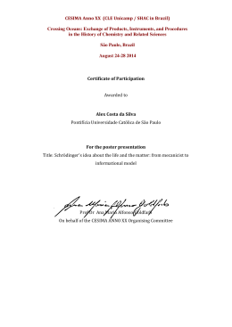
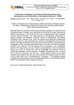
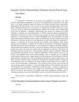
LIFE HISTORY MOVEMENTS AND SPAWNING OF SÃO FRANCISCO
RIVER FISHES, BRAZIL
A Dissertation Presented
by
ALEXANDRE LIMA GODINHO
Submitted to the Graduate School of the
University of Massachusetts Amherst in partial fulfillment
of the requirements for the degree of
DOCTOR OF PHILOSOPHY
May 2005
Wildlife and Fisheries Conservation
© Copyright by Alexandre Lima Godinho 2005
All Rights Reserved
LIFE HISTORY MOVEMENTS AND SPAWNING OF SÃO FRANCISCO
RIVER FISHES, BRAZIL
A Dissertation Presented
by
ALEXANDRE LIMA GODINHO
Approved as to style and content by:
__________________________________________
Boyd Kynard, Chair
__________________________________________
William E. Bemis, Member
__________________________________________
Alexander J. Haro, Member
__________________________________________
Francis Juanes, Member
________________________________________
Matthew J. Kelty, Department Head
Department of Natural Resources Conservation
DEDICATION
To my beloved son Henrique and parents Hugo and Ica
ACKNOWLEDGMENTS
I am deeply grateful for all institutions and individuals that made this study
possible. I thank the Brazilian people via PADCT/CIAMB agreement number
62.0088/98-2; Banco do Nordeste do Brasil; Cemig; Colônia de Pescadores de Pirapora;
CNPq; Estação de Hidrobiologia e Piscicultura de Três Marias; FAPEMIG; Funbio;
Fundação Boticário; PMMG; Pós-Graduação em Ecologia, Conservação e Manejo de
Vida Silvestre da UFMG; Pró-Reitoria de Pesquisa da UFMG; SAAE Buritizeiro;
SAAE Pirapora; S. O. Conte Anadromous Fish Research Center (USGS); UHE Três
Marias; and US Fish and Wildlife Service.
I also thank the commercial fishers of Três Marias and Pirapora, Luiz Augusto
B. Almeida, Carlos B. M. Alves, William Bemis, Gilberto Cintron, Capt. Arley
Ferreira, Marcelo F. Fonseca, Sandra Francischetti, Hugo P. Godinho, Alex Haro, Luz
F. Jiménez, Francis Juanes, Ivana R. Lamas, Regina S. Lopes, Carlos A. K. Miranda,
Gisele V. M. A. Paula, Antonio Procópio S. Rezende, Mário Ribeiro, Meiry Santos,
Norberto A. Santos and sons, Luiz Fernando B. M. Silva, Paulo Henrique L. Sousa,
Vasco C. Torquato, and Bill Whitmore. I am specialy thankful for Boyd Kynard for his
wise guidance and for his extraordinary good will to help me since our very first
contact. If by mistake, I forgot to thank you, be sure that I am very grateful for your
help too. I had a Brazilian government scholarship - CAPES – Brazil.
v
ABSTRACT
LIFE HISTORY MOVEMENTS AND SPAWNING OF SÃO FRANCISCO RIVER
FISHES, BRAZIL
MAY 2005
ALEXANDRE LIMA GODINHO, B.S., UNIVERSIDADE FEDERAL DE MINAS
GERAIS
M.S., UNIVERSIDADE FEDERAL DE MINAS GERAIS
Ph.D., UNIVERSITY OF MASSACHUSETTS AMHERST
Directed by: Professor Boyd Kynard
The São Francisco River (SFR), a floodplain river southeast of the Amazon
River, provides commercial and recreational fishing for thousands of people, but
fisheries have collapsed in the last decade. During 32-months, I radio-tracked 37
curimbatás (Prochilodus argenteus, Characidae, 0.8–2.9 kg) and 24 surubims
(Pseudoplatystoma corruscans, Pimelodidae, 9.5–29.0 kg), two important commercial
and recreational fishes. I did the study to characterize their migratory style and to
determine if the cool hypolimnetic discharge from an upstream dam (Três Marias
Reservoir, TMR) would block their upriver migration. I also made a conceptual model
of the biological, river, dam, reservoir, and economic factors for a supplemental water
release (SWR) to enhance SFR fisheries using a release from TMR. Migratory style of
both species was dualistic with resident and migratory individuals. Home range was 1–
127 km for curimbatá and 1–210 km for surubim. The most important spawning area for
curimbatás was the SFR mainstem at its juncture with the Abaeté River mouth, and for
surubims, the most important spawning area was the mainstem at Pirapora Rapids. Pre-
vi
spawning adults of both species staged at or near the spawning grounds. Some
curimbatás and surubims homed to pre-spawning staging areas and to spawning areas.
Some curimbatás also homed to non-spawning areas. The movements and thermal
fluctuations experienced by both fishes showed they are eurythermal with a broad shortterm temperature variation tolerance. Also, water discharged from dams that is < 5oC
cooler than ambient river water will not disrupt their migrations. The best date for a
SRW is when there is a natural flood, which triggers spawning. The SWR will intensify
the natural flood, cover a greater floodplain area, and increase survival of early life
stages of fish. The TMR frequently impounded enough water for SWR only in the
second half of the fish spawning season (January–March). Lost revenue at TMR
depended on release volume and ranged from US$ 0.493 million to US$ 3.452 million
for the actual power rate. However, SWR could increase commercial fisheries income
an estimated US$ 4.468 million. Planned construction of 16 dams in the mainstem and
tributaries downstream from TMD will greatly affect curimbatá and surubim migrations
and spawning habitat, extirpate populations, and eventually reduce their abundance.
vii
TABLE OF CONTENTS
Page
ACKNOWLEDGMENTS ................................................................................................ v
ABSTRACT..................................................................................................................... vi
LIST OF TABLES..........................................................................................................xii
LIST OF FIGURES .......................................................................................................xiii
CHAPTER
1.
INTRODUCTION ................................................................................................ 1
1.1. Brazilian Fish Diversity and its Social Importance ....................................... 1
1.2. Life History Movement, Dams, and Fish Passage......................................... 2
1.3. Fish Spawning and Supplemental Water Release.......................................... 2
1.4. Objectives ...................................................................................................... 3
1.5. Study Area ..................................................................................................... 5
1.6. Study Fishes ................................................................................................... 6
2.
MIGRATION AND SPAWNING OF CURIMBATÁ (Prochilodus
argenteus, PROCHILODONTIDAE) IN THE SÃO FRANCISCO RIVER,
BRAZIL .............................................................................................................. 13
2.1. Introduction.................................................................................................. 13
2.2. Study Area ................................................................................................... 15
2.3. Methods ....................................................................................................... 16
2.3.1. Tagging and tracking .................................................................... 16
2.3.2. Data analysis ................................................................................. 19
2.4. Results.......................................................................................................... 21
2.4.1. Tagging mortality and tag failure ................................................. 21
2.4.2. Disappearance of tagged fish ........................................................ 22
2.4.3. TM fish.......................................................................................... 22
2.4.4. Pontal fish ..................................................................................... 23
2.4.5. Cilga fish....................................................................................... 24
2.4.6. Migration to Pontal ....................................................................... 24
2.4.7. Visits to Pontal from pre-spawning staging areas ........................ 25
2.4.8. Abaeté River conditions during visits........................................... 26
2.4.9. Pre-spawning staging areas near Pontal........................................ 27
2.4.10. Mainstem and tributaries use ...................................................... 27
viii
2.4.11. Homing fidelity........................................................................... 28
2.4.12. Home range................................................................................. 29
2.4.13. Spawning during successive years.............................................. 30
2.5. Discussion .................................................................................................... 30
2.5.1. Spawning grounds......................................................................... 30
2.5.2. Visits to Pontal.............................................................................. 32
2.5.3. Pre-spawning staging area ............................................................ 33
2.5.4. Spawning periodicity .................................................................... 34
2.5.5. Non-spawning grounds ................................................................. 34
2.5.6. Homing ......................................................................................... 35
2.5.7. Home range................................................................................... 36
2.5.8. Juvenile migration......................................................................... 38
2.5.9. Metapopulation ............................................................................. 38
2.5.10. Population structure .................................................................... 40
2.5.11. Conceptual model ....................................................................... 41
2.6. Conservation and Management ................................................................... 43
3.
MIGRATION AND SPAWNING OF SURUBIM (Pseudoplatystoma
corruscans, PIMELODIDAE), IN THE SÃO FRANCISCO RIVER,
BRAZIL. ............................................................................................................. 59
3.1. Introduction.................................................................................................. 59
3.2. Study Site ..................................................................................................... 60
3.3. Methods ....................................................................................................... 61
3.3.1. Tagging and tracking .................................................................... 61
3.3.2. Data analysis ................................................................................. 63
3.4. Results.......................................................................................................... 66
3.4.1. Characteristics of tracked surubims.............................................. 66
3.4.2. Locations during spawning and non-spawning seasons ............... 66
3.4.3. Tracks at PR reach ........................................................................ 67
3.4.4. Tracks of pre-spawning staging fish ............................................. 68
3.4.5. Tracks downstream from PR ........................................................ 68
3.4.6. Migration to Pontal ....................................................................... 69
3.4.7. Mainstem and tributary tracks ...................................................... 69
3.4.8. Home range................................................................................... 69
3.4.9. Homing ......................................................................................... 70
3.4.10. Time of migration ....................................................................... 71
3.4.11. Sprint migration .......................................................................... 71
3.4.12. Use of TMD reach ...................................................................... 71
ix
3.5. Discussion .................................................................................................... 72
3.5.1. PR spawning ground ..................................................................... 72
3.5.2. Spawning downstream of PR........................................................ 73
3.5.3. Pontal spawning ground................................................................ 73
3.5.4. Multiple visits ............................................................................... 74
3.5.5. Pre-spawning staging areas........................................................... 75
3.5.6. Spawning season........................................................................... 76
3.5.7. Non-spawning grounds ................................................................. 76
3.5.8. TM reach....................................................................................... 77
3.5.9. Homing ......................................................................................... 77
3.5.10. Sprint migration .......................................................................... 78
3.5.11. Dualistic migration ..................................................................... 79
3.5.12. Conceptual model of migration .................................................. 80
3.5. Conservation and Management ................................................................... 82
4.
RESPONSE OF TWO BRAZILIAN FISHES TO ARTIFICIALLY COOL
WATER DURING UPRIVER MIGRATION.................................................... 98
4.1. Introduction.................................................................................................. 98
4.2. Methods ..................................................................................................... 100
4.2.1. Thermal environment.................................................................. 100
4.2.2. Radio-tracking ............................................................................ 101
4.3. Results........................................................................................................ 102
4.3.1. Thermal environment.................................................................. 102
4.3.2. Fish movements .......................................................................... 104
4.4. Discussion .................................................................................................. 104
4.4.1. Thermal environment.................................................................. 104
4.4.2. Thermoregulation of surubim and curimbatá ............................. 106
5.
SUPPLEMENTAL WATER RELEASES FOR FISHERIES
RESTORATION IN A BRAZILIAN FLOODPLAIN RIVER: A
CONCEPTUAL MODEL ................................................................................. 113
5.1. Introduction................................................................................................ 113
5.2. Fisheries and Study Site............................................................................. 116
5.2.1. Fisheries ...................................................................................... 116
x
5.2.2. Três Marias Dam and the river downstream............................... 116
5.3 Methods ...................................................................................................... 117
5.3.1. What is the best release date? ..................................................... 117
5.3.2. How much water will be released? ............................................. 119
5.3.3. What is the pattern of impoundment and how much
impounded water will be released?........................................... 119
5.3.4. What is the lost revenue to the power plant associated with
SWR? ........................................................................................ 120
5.3.5. What is the relationship between SWR and fisheries value?...... 120
5.5. Results........................................................................................................ 121
5.5.1. What is the best release date? ..................................................... 121
5.5.2. How much water will be released? ............................................. 124
5.5.3. What is the pattern of impoundment and how much
impounded water will be released?........................................... 124
5.5.4. What is the lost revenue to the power plant associated with
SWR? ........................................................................................ 125
5.5.5. What is the relationship between SWR and fisheries value?...... 125
5.6. Discussion .................................................................................................. 125
5.6.1. What is the best release date? ..................................................... 126
5.6.2. How much water will be released? ............................................. 130
5.6.3. What is the pattern of impoundment and how much
impounded water will be released?........................................... 131
5.6.4. What is the lost revenue to the power plant associated with
SWR? ........................................................................................ 133
5.6.5. What is the relationship between SWR and fisheries value?...... 133
6.
CONCLUSIONS............................................................................................... 149
BIBLIOGRAPHY......................................................................................................... 152
xi
LIST OF TABLES
Table
Page
2.1. Fish characteristics and tracking summary of radio-tagged curimbatá in
the São Francisco River, 2001–2003. ..................................................... 46
3.1. Fish characteristics and tracking summary of 24 radio-tagged female
surubims in the São Francisco River, 2000–2003.. ................................ 85
3.2. Sprint migrations (pre-spawning staging and non-spawning) of five
surubims in the São Francisco River.. .................................................... 87
4.1. Short- and long-term (annual) thermal-amplitude of the Abaeté River
and São Francisco River at Pirapora Rapids......................................... 108
4.2. Surubim and curimbatá tracked moving upstream past Pontal into cooler
mainstem São Francisco River water.................................................... 109
5.1. Spearman correlation matrix of egg density, water level at three gauging
stations (Pirapora, TM = Três Marias, and Abaeté), conductivity
(Cond), turbidity (Turb), and temperature (Temp) in the São
Francisco River. .................................................................................... 135
5.2. Spearman correlation matrix of egg density, water level at four gauging
stations (Guacuí, VP = Várzea das Palmas, Licinio, and Paraúna),
pH, conductivity (Cond), turbidity (Turb), and temperature
(Temp) in the Velhas River.. ................................................................ 136
5.3. Strongest cross-correlation between daily mean density of the
ichthyoplankton life stage and water level at gauging stations in
the São Francisco and Velhas basins. ................................................... 137
5.4. The volume of water released from Três Marias Reservoir during
supplemental water released (SWR) of various durations.................... 138
xii
LIST OF FIGURES
Figure
Page
1.1. Map of the São Francisco River Basin showing the three major
reservoirs (TMD = Três Marias Dam, SD = Sobradinho Dam, ID
= Itaparica Dam), future hydropower developments in the
mainstem (
) and some of the major riverine cities (TM =
Três Marias, PP = Pirapora, SR = São Romão, JN = Januária, and
XX = Xique-Xique). ............................................................................... 10
1.2. Curimbatá (Prochilodus argenteus)................................................................... 11
1.3. Surubim (Pseudoplatystoma corruscans). ......................................................... 12
2.1. The study area for curimbatá in the São Francisco River Basin........................ 48
2.2. Curimbatá movements in the São Francisco River Basin. Fish were
grouped in three clusters (TM = Três Marias, Pontal, and Cilga)
accord to the river reach in which they were located more
frequently during the spawning season................................................... 49
2.3. Monthly frequency of detection of tagged curimbatá by the Pontal
receiver.................................................................................................... 50
2.4. Frequency of visits by curimbatás to Pontal in the São Francisco
mainstem during varying discharge and temperature conditions in
the Abaeté River mouth where it joins the São Francisco River. ........... 51
2.5. Migration of LS Cilga curimbatá female 69 in the São Francisco River .......... 52
2.6. Migration of likely LS curimbatás (73, 81 and 154) in the São Francisco
River........................................................................................................ 53
2.7. Migration of LS Cilga curimbatá female 57 in the São Francisco River .......... 54
2.8. Frequency of occurrence of 19 curimbatás among 10-km long segments
of the mainstem São Francisco River and two tributaries ...................... 55
2.9. Total home range of 19 curimbatás (12 females and 7 males) tracked
during the spawning and non-spawning seasons of 2001, 2001–
2002, and 2002–2003.............................................................................. 56
2.10. Non-spawning home range of 21 curimbatás (16 females and 5 males)
during 2001, 2002 and 2003. .................................................................. 57
xiii
2.11. Metapopulation structure and conceptual model of life history
movements of curimbatás in the São Francisco River between
Três Marias Dam (TDM) and the city of Januária.................................. 58
3.1. The study area for surubim in the São Francisco River Basin........................... 88
3.2. Surubim activity in the São Francisco River Basin ........................................... 89
3.3. Frequency of visits of surubims to Pontal during conditions of the São
Francisco River. ...................................................................................... 90
3.4. Movements of surubims 24 and 36 in the São Francisco River near PR
(Pirapora Rapids, dashed line). ............................................................... 91
3.5. Migration of surubims 40 and 225 to spawning and non-spawning
grounds in the São Francisco River ........................................................ 92
3.6. Frequency of occurrence of surubim in 20-km long segments of the São
Francisco and Velhas River .................................................................... 93
3.7. Total home range (top panel) and non-spawning home range (bottom
panel) of surubims in the São Francisco (black bar) and Velhas
(dotted bar) rivers.................................................................................... 94
3.8. Migration of the surubims 22, 24, 26, and 30 in the São Francisco River. ....... 95
3.9. Model of generalized pattern of fish migration (Northcote 1978) which
includes pre-spawning staging habitat.................................................... 96
3.10. Spawning (dark circle; PR = Pirapora Rapids) and non-spawning
(diagonal lines buffer) grounds of curimbatá in the São Francisco
River Basin downstream TMD (Três Marias Dam) ............................... 97
4.1. Map of the São Francisco River basin showing the study area
downstream of Três Marias Dam (TMD) to Pirapora Rapids .............. 110
4.2. Hydrographs of the Abaeté River (32 km upstream from the mouth) and
at three locations in the São Francisco River: TM = Três Marias,
downstream of Pontal after the mixing of the Abaeté River, and
PR = Pirapora Rapids............................................................................ 111
4.3. Daily mean temperature of the Abaeté River (at the mouth), and at three
locations in the São Francisco River: Firmino (5 km upstream of
Pontal), downstream of Pontal after the mixing of the Abaeté
River, and PR = Pirapora Rapids. ......................................................... 112
xiv
5.1. Map of the São Francisco and Velhas rivers upstream the
ichthyoplankton sampling sites (dashed arrows) .................................. 139
5.2. Daily water level (WL) in the São Francisco and Velhas rivers from late
November to early February during two consecutive spawning
seasons (1998–1999 and 1999–2000)................................................... 140
5.3. Daily mean density of ichthyoplankton life stages in the São Francisco
(top panel) and Velhas (bottom panel) rivers during two
consecutives spawning seasons (1998–1999 and 1999–2000) ............. 141
5.4. Mean and one standard deviation of total ichthyoplankton density in the
São Francisco and Velhas rivers from late November to early
February during two consecutive spawning seasons (1998–1999
and 1999–2000) .................................................................................... 142
5.5. Percentage of days with flood (water level at any day at least 20 cm
greater than the day before) from November to March in the
Abaeté and Velhas rivers ...................................................................... 143
5.6. Daily mean egg densities in the São Francisco (top panels) and Velhas
(bottom panels) rivers near their junction and the daily water
level (WL) in the biggest upstream tributary from late November
to early February during two consecutive spawning seasons
(1998–1999 and 1999–2000). ............................................................... 144
5.7. Mean and one standard deviation of egg densities in the São Francisco
and Velhas rivers near their junction .................................................... 145
5.8. Monthly volume of water (mean and range) impounded by Três Marias
Reservoir, 1976–2003. .......................................................................... 146
5.9. Percentage of the flood volume (mean and range) in the daily live
storage of Três Marias Reservoir for flood duration of 2–8 days
in November to March .......................................................................... 147
5.10. Três Marias power plant lost revenue (R) due to supplemental water
releases for durations of 2–8 days and three power rates. .................... 148
xv
CHAPTER 1
INTRODUCTION
1.1. Brazilian Fish Diversity and its Social Importance
Freshwater fishes are one of the marvels of Brazil’s natural resources. With
3,000+ known species, Brazil has the richest freshwater fish diversity on Earth
(McAllister 1977). The numerous wonderful ornamental fishes like the popular neontetra, the huge aggressive recreational ‘dourado’ (Salminus spp.), the giant ‘pirarucu’
(Araipama gigas), the electric eel (Electrophorus electricus), the legendary ‘piranha’
(Pygocentrus spp.), the highly prized foodfish ‘surubim’ (Pseudoplatystoma), the
‘candiru’ (Vandellia cirrhosa), which is notorious for swimming into human urethra,
make this a unique fish fauna.
Besides their diversity, Brazilian freshwater fishes provide food and jobs for
millions of people all over the country. From 1984 to 1998, freshwater fisheries
landings ranged from 152 to 183 thousand tons per year, numbers that do not actually
represent the real magnitude of the fisheries due to the scattered nature of landings
(Fischer et al. 2000).
The São Francisco River (SFR) is a medium sized watershed located near the
east coast of South America, southeast of the Amazon River (Figure 1.1). It was once
one of the fisheries hot spots in Brazil. Moojen (1940) wrote that its fisheries were a
miracle and Menezes (1956) compiled several amazing reports of abundant fisheries
during the first half of the last century. Several fishers’ villages flourished along the
riverbanks and fisheries were the main livelihood of thousands of commercial fishers.
1
Nowadays, hundreds of thousands of people still drive each year to the river for
recreational fisheries. Numerous establishments like hotels, motels, restaurants, sport
fishing clubs, and stores depend on the recreational fishery as the primary or secondary
sources of income.
Despite the lack of systematic records of the São Francisco’s fisheries, there is
clear evidence that the fisheries have collapsed during recent years. Catch reduction has
been frequently reported in the media, and anglers and commercial fishers complain
often about it. Commercial fishers groups have requested changes in fisheries
regulations that allow catching smaller fish. One of the strongest pieces of evidence of a
collapse is the reduction in capture per unit of effort per commercial fishing boat at
Pirapora, an important fishing area in the middle course of the river at river km (rkm)
1,978. The catch has declined from 11.7 kg.fisher-1.day-1 in 1987 to 3.1 kg.fisher-1.day-1
in 1999 (Godinho et al. 1997, Godinho pers. obs.). Surubim, which accounted for 86%
of the biomass caught in 1987, represented only 27% in the 1997 catch.
1.2. Life History Movement, Dams, and Fish Passage
As in the rest of the world, where many commercially important freshwater
fishes are migratory (Wootton 1990), the most important commercial and game fish
species of the SFR are migratory. Despite their importance, their migratory behavior is
almost entirely unknown. Two attempts to study adult migrations using mark and
recapture methods provided only superficial insights (Paiva and Bastos 1982, Sato and
Godinho 2003). Therefore, migratory routes, time of migration, and location of
spawning and feeding grounds have not been described.
2
The SFR Basin hydropower potential is 26.3 GW, with 10.5 GW already
developed (ANEEL 2002). All major developments are in the mainstem and most are in
the lower section of the river. Only one major dam, Três Marias Dam (TMD), was built
in the upper section of the mainstem (Figure 1.1). Within 506 km downstream of TMD,
four dams are planned that will convert that entire reach of the mainstem into a series of
large reservoirs (Figure 1.1). In the free-flowing Abaeté River, there are nine potential
sites for dams and in the Velhas River, the second biggest tributary, three dam sites.
There is no fish passage in any SFR dam.
The efficiency of a fish passage depends on free access of the migrants to the
downstream passage entrance, which is always in the tailrace below the dam. However,
the tailrace water at some dams may be cool enough to act as a movement barrier. For
example, at TMD, located in the SFR at rkm 2,109 (Figure 1.1), the water intake is
located at the hypolimnetic layer of the reservoir where the water is 5–7 oC cooler than
the surface water during the rainy season (Esteves et al. 1985). Consequently, the
tailrace water is also cool. Eventually, downstream of the dam the water temperature
increases after receiving warmer water from tributaries (Sampaio and López 2003).
Thus, if the Três Marias’ tailrace discharge really acts as a physical barrier for migrants,
this could preclude any attempt to provide an upstream passage for fishes at TMD or
similar dams.
1.3. Fish Spawning and Supplemental Water Release
Many studies emphasize the importance of floodplain lakes to the rearing
success and recruitment of many species of migratory fishes, including the fishes in the
3
SFR (Bonetto et al. 1969, Godoy 1975, Sato et al. 1987, Carolsfeld et al. 2003, Pompeu
and Godinho 2003). The SFR has abundant floodplain lakes, but the largest of these is
the 16 km wide floodplain at the city of Januária (rkm 1,700). It reaches a width of tens
of km close to the city of Xique-Xique (rkm 1,062; Sato and Godinho 2003).
The migratory fishes in the SFR are broadcast spawners that spawn nonadhesive, semi-buoyant eggs that hatch in less than one day during the rainy season
(October–March; Sato et al. 2003a, b). Spawning timing, characteristics of the eggs,
and characteristics of the early life stages are adaptations that increase the probability
that early life stages will reach floodplains lakes. Consequently, spawning timing of is a
critical moment for recruitment.
The lack of big floods during the last decade may be the major cause of the
fishery collapse of the SFR (Godinho and Godinho 2003). The last major flood
occurred in 1992 when the water level reached 11.8 m at the city of São Romão (rkm
1,837). Since then, the floods have been lower, ranging from 5.9 to 8.7 m. The lack of
major floods could reduce fisheries yield by preventing eggs and larvae from reaching
floodplain lakes or by preventing young fish in the floodplain lakes from returning to
the river, thereby increasing mortality due to predation and desiccation. Moreover, lack
of floods reduces the flood pulse effect, which is the principal driving force responsible
for the existence, productivity, and interactions of the major biota in floodplain river
systems (Junk et al. 1989). The collapse of the fishery for Prochilodus lineatus in the
Pilcomayo River in Bolivia during the 1990s was attributed to decreased river discharge
due to the El Niño phenomenon (Smolder 2000).
4
Control of river water discharge by TMD was also suggested as a possible cause
for the collapse of the São Francisco fisheries (Godinho and Godinho 1994). River
discharge is controlled to avoid flooding as well as to improve commercial navigation
and tourism. Spawning success and recruitment of migratory fishes, however, most
probably depends on floods that no longer occur with the same frequency or intensity.
Flow regulation is perhaps the most pervasive change by humans on rivers worldwide
(Stanford et al. 1996).
Supplemental water release (SWR) has been used for fisheries restoration (Petts
1989, Welcomme 1989, Orth and White 1993, Godinho 1993, Swales 1994).
Welcomme (1989) suggested that water discharge from dams could be released to
provide a flood to stimulate fish spawning. He mentioned three cases in Africa where
discharge was manipulated to enhance fisheries. Riverine fishes successfully spawned
after flood augmentation in the Pongolo River, South Africa. Juveniles of several
species appeared in the floodplains of the Zambezi River, Zambia/Zimbabwe, after
artificial floods, and Welcomme (1989) concluded that artificial releases of water from
dams could stimulate spawning of riverine fishes.
1.4. Objectives
The present multi-year research study is on basic and applied issues of
migratory fishes in the SFR. It addresses topics related to the life history migrations of
curimbatá, Prochilodus argenteus (= Prochilodus marggravii) Spix and Agassiz 1829
(Characiformes, Prochilodontidae) and surubim, Pseudoplatystoma corruscans (Spix
5
and Agassiz 1829) (Siluriformes, Pimelodidae), two of the most important commercial
and recreational SFR fish species. It also addresses SWR from TMD to restore fisheries.
For curimbatá, I used radio-telemetry to identify migrations, determine home
ranges, identify spawning and non-spawning grounds, determine if fish homed, and
determine the timing of spawning relative to river conditions. I also developed a
conceptual model of migration that would contribute to understanding the species’ life
history (Chapter 2).
For surubim, I used radio-telemetry to identify river reaches used for spawning,
pre-spawning staging and non-spawning activities and to determine home range,
identify migration timing, determine detailed use of spawning area, determine if fish
homed, and measured migratory ground speed. I used these data to develop a
conceptual model of migration and spawning for the species (Chapter 3).
For both species, I radio-tracked fish movements at the junction of the cooler
mainstem water with the warmer water of the Abaeté River to test the hypothesis that
the cooler TMD discharge blocked upstream fish migration (Chapter 4).
I gathered biological data on spawning timing and river condition and
information on TMD releases and storage, value of water for generation, and historical
flooding patterns to make a conceptual model of the biological, river, dam and
reservoir, and economic factors for a SWR in the SFR (Chapter 5).
1.5. Study Area
The SFR is located in the east coast of South America southeast of the Amazon
River between the coordinates 13o and 21o L and 36o and 48o W (Figure 1.1). It is a
6
medium sized basin of 631,000 km2. It drains 7.4% of the Brazilian territory and flows
2,680 km generally northward (Paiva 1982). The climate is hot and humid (type Aw,
Köppen system) with a dry winter in the upper portions of the basin upstream of rkm
1,250 (Bernardes 1951). High water discharge occurs during summer whereas low
water occurs in winter. Mean river discharge is 3.150 m3.s-1, seven times larger than the
discharge of the Connecticut River, USA (Boyd 1976). Between the cities of Três
Marias and Pirapora, river water temperatures range from 18–29 oC, conductivity from
36–76 µS cm-1, and pH from 6.3–8.2 (Sato and Godinho 2003). The river in that reach
is characterized by high gradient, fast current, rocky bottom, and frequent short rapids.
The Pirapora Rapids is 1,000 m long and 8 meters high. Downstream of Pirapora, the
river gradient is low, current is slow, bottom is mostly sand, floodplain is wider, and
rapids are absent.
There are 10 major hydroelectric developments in the basin, six of these are in
the mainstem. Três Marias (rkm 2,109) and Sobradinho (rkm 750) dams are the biggest.
The TMD has a flooded area of 1,042 km2 and was filled in the early 1960s. Sobradinho
Dam was built in the 1970s and has a flooded area of 5,805 km2. These manmade
reservoirs are respectively, 13 and 72 times bigger than the area of Quabbin Reservoir
(80.3 km2) in Massachusetts, USA.
The study area is the section of the SFR Basin between TMD and Sobradinho
Reservoir. The core area is restricted to the 276 km directly downstream of TMD. The
1,090 km long section between TMD and Sobradinho Reservoir is the longest free
flowing section in the basin. None of these tributaries in this part of the basin contain
flood control facilities. Most of the biggest tributaries and floodplain lakes occur there.
7
The biggest tributaries are Velhas (rkm 1,952), Paracatu (rkm 1,866), Urucuia (rkm
1,719), Carinhanha (rkm 1,543), Corrente (rkm 1,395), and Grande (rkm 1,134). The
floodplain is relative narrow in the first 247 km downstream from TMD. It increases in
width after the mouth of the Paracatu River (rkm 1,866), and at the city of Januária
(rkm 1,700), it is 16 km wide and reaches tens of km at the city of Xique-Xique (Sato
and Godinho 2003). There is no information on how many floodplain lakes exist in the
Três Marias-Sobradinho reach, but it may be thousands.
1.6. Study Fishes
Curimbatá (Figure 1.2) is a member of the family Prochilodontidae endemic to
the SFR (Sato et al. 1996). Members of this family can be readily distinguished by their
fleshy lips with two series of numerous, relatively small, falciform or spatulate teeth,
movably attached to the lips (Castro and Vari 2003). Prochilodontids have bean-shaped
body, a protractile mouth forming a sucking disc, and a pre-dorsal spine (Gery 1975).
Prochilodus argenteus is an iliophagus fish that reaches 15 kg and is the largest species
of its family (Sato et al. 1996). Adult curimbatás have a dorsal fin plain, 41–45 lateral
line scales and body depth 2.5–2.7 times in the standard length (Gery 1975). It is one of
the most common big fish in the SFR and a second/third grade fish for commercial
fisheries. It was only a non-game fish, but new angling techniques have changed that.
Curimatá is a long distance migratory fish (Sato and Godinho 2003), total spawner
(Bazzoli 2003) that broadcasts many non-adhesive eggs (252 eggs per g of body weight;
Sato et al. 2003a) from November to February (Bazzoli 2003). Females have a high
gonadosomatic index (mean of 24%), non-hydrated egg have diameter of 1.6 mm, egg-
8
hatching occurs around 19 hours after fertilization at 24 oC, and larval length at
hatching is 4.2 mm (Sato et al. 2003a, b). The larval stage lasts for four days (Godinho
et al. 2003).
Surubim (Figure 1.3) is a catfish in the family Pimelodidae. Pimelodids do not
have any unique externally visible characteristics, but can be distinguished from other
South American siluriforms by a combination of features (Lundberg and Littmann
2003). Pseudoplatystoma has a long depressed snout with four moderately long
maxillary barbels. The width of the mouth is about equal to the maximum width of the
head and less than the head length. The palatal teeth are arranged in two patches in the
form of a curved and elongated comma (Burgess 1989). Surubim is blackish dorsally
and white ventrally with dark spots all over the body, except ventrally and on most of
the head. Surubim occurs in the São Francisco and Paraná-Paraguay-Uruguay basins.
This piscivorous fish is one of the largest neotropical fishes growing to 3.3 meters in
length (Ihering 1934); such a fish would weigh 435 kg according to the species’
weight–length equation (Godinho et al. 1997). However, a fish that weight has never
been documented. Sato et al. (2003a) mentione that the maximum weight of the species
in the SFR Basin is 120 kg. Like curimbatá, surubim is a long distance migratory fish
(Sato and Godinho 2003), total spawner (Bazzoli 2003) that broadcasts many nonadhesive eggs (126 eggs per g of body weight; Sato et al. 2003a) from November to
January (Godinho et al. 1997, Brito and Bazzoli 2003). It reaches sexual maturity at a
body length of 55 cm (Lamas 1993). Gonadosomatic index of females is low (3%;
Lamas 1993), diameter of non-hydrated egg is 1.0 mm (Sato et al. 2003b), and eggs
hatch in 20 hours at 24.4 oC. The larval stage lasts for four days (Godinho et al. 2003).
9
XX
d
an
Gr
.
eR
R.
Corrente
Carinhan
h a R.
JN
uia
uc
Ur
R.
Brazil
SR
Ab
ae
té
PP
TM
.
sR
lha
R.
.
Ve
R
atu
rac
Pa
Figure 1.1. Map of the São Francisco River Basin showing the three major reservoirs
(TMD = Três Marias Dam, SD = Sobradinho Dam, ID = Itaparica Dam), future
hydropower developments in the mainstem (
) and some of the major riverine cities
(TM = Três Marias, PP = Pirapora, SR = São Romão, JN = Januária, and XX = XiqueXique).
10
Figure 1.2. Curimbatá (Prochilodus argenteus).
11
Figure 1.3. Surubim (Pseudoplatystoma corruscans).
12
CHAPTER 2
MIGRATION AND SPAWNING OF CURIMBATÁ (Prochilodus argenteus,
PROCHILODONTIDAE) IN THE SÃO FRANCISCO RIVER, BRAZIL
2.1. Introduction
Fishes of the genus Prochilodus forage on detritus and periphyton and inhabit
many South American rivers where they are an important fisheries resource (Castro and
Vari 2003). Prochilodus argenteus (common name, curimbatá) is endemic to the São
Francisco River, a large basin southeast of the Amazon River. Curimbatás grow to a
maximum body weight of 15 kg (Sato et al. 1996) and are sexually mature at 3 years
(Santos and Barbieri 1991). They are one of the most important recreational and
commercial fish in the basin (Franco de Camargo and Petrere 2001, Godinho et al.
2003a). Despite the importance of curimbatás to the São Francisco River fisheries, most
aspects of their life history (especially migrations, home range, and spawning locations)
are not understood. This information is critically needed to evaluate the environmental
impacts of the many dams and large reservoirs that are planned for the mainstem and
tributaries.
Some information on spawning and early-life history of curimbatá is available.
During spawning, a female broadcasts hundreds of thousands of small, non-adhesive
eggs in a single batch in the rainy season between November and February (Bazzoli
2003, Sato et al. 2003b). Eggs are semi-buoyant, drift downstream with river flow
(Chapter 5), and hatch in 19 h at 24 oC (Sato et al. 2003b). Drifting eggs and larvae are
in the water column and density is highest during floods when spawning occurs
(Chapter 5). During flooding, larvae drift into floodplain lakes, which are important
13
nursery grounds for early juveniles (Sato et al. 1987, Pompeu and Godinho 2003).
Some larvae may also rear in the river, but data are lacking. Preliminary observations
suggest that at some point in development, juveniles migrate upriver in the dry season
to join adults (Godinho pers. obs.).
The present conceptual model of adult Prochilodus spp. migration and home
range is from mark-recapture studies on P. lineatus (= P. scrofa and P. platensis) in the
Paraná–Paraguay River basin of Brazil and Argentina during the 1950s–1960s (Godoy
1959, Godoy 1962, Bonetto 1963, Bonetto and Pignalberi 1964, Bonetto et al. 1971,
Godoy 1975). Prochilodus lineatus in the upper Paraná River basin, a neighbor basin of
the São Francisco River, migrates a maximum round trip distance of 1,300 km between
feeding grounds in the mainstem and spawning grounds in a tributary (Godoy 1975,
Toledo et al. 1986). Upriver pre-spawning migration occurs during September–
December and spawning occurs during November–February, mostly in a 4 km reach
downstream of a waterfall (Godoy 1954). During spawning, thousands of noisy (males
have a mating call), schooling adults swim at the water's surface, a phenomenon locally
called ‘rodada’ (Schubart 1943). Thirty-one of 43 ‘rodadas’ studied by Schubart (1954)
occurred when the river was flooding.
In the São Francisco River, two mark-recapture studies on curimbatás provide
some information on home range of adults. Fish (presumably adults) from different
reaches were quite different for home range, i.e., 1,100 km maximum for fish tagged in
the lower region by Jucá (Sato and Godinho 2003) and 250 km for fish tagged in the
upper region (Paiva and Bastos 1982). The few recaptures in these studies did not
14
provide insight on size of spawning vs. non-spawning home range, adult migrations,
and did not identify location of any spawning grounds.
Migrations of several South American fishes have been studied mostly using
mark-recapture (Petrere 1985, Carolsfeld et al. 2003). Telemetry rarely has been used in
South America to study migratory fish (Mochek et al. 1991). I radio-tracked curimbatás
from three reaches in the São Francisco River for 2.5 years and I was even able to
follow some individuals for two spawning seasons. At the time of tagging, I identified
the sex and reproductive stage to link movements and behavior to reproductive stage.
My objectives were to identify migrations, determine home ranges, identify spawning
and non-spawning river reaches, determine timing of spawning relative to river
conditions, and develop a conceptual model of migration that would contribute to
understanding the species’ life history.
2.2. Study Area
The São Francisco River is a large river on the east coast of South America that
flows mostly northward 3,160 km and drains a basin of 645,067 km2 (Kohler 2003). The
reach where I tagged all fish and tracked fish most intensively extended 129 km
downstream from Três Marias Dam (TMD) to Pirapora Rapids (PR; Figure 2.1). This
reach of river has a high gradient with fast current, rapids, and runs. The bottom is
mostly rocky. There are only a few narrow floodplains that seldom flood because of
regulated flow at TMD. Within 506 km downstream of TMD, four dams are planned
that will convert that segment of the mainstem into a series of big reservoirs. Abaeté
River is the largest of the three major tributaries in the TMD-Pirapora reach. It drains an
15
area 2.6 times larger than the combined areas of the other two tributaries which are the
Janeiro and Formoso rivers. In the free-flowing Abaeté River, there are nine potential
sites for dams. At PR, the river level declines 8 m over a distance of 1 km at a steep
rapids. Downstream of PR, river gradient is low, current is slow, bottom is generally
sand, and the channel meanders. Many wide floodplains are present, mostly below the
Paracatu River mouth at river km (rkm) 1,866.
Physical and chemical quality of the river mainstem in the study area reflects the
hypolimnetic discharge of Três Marias Reservoir, winter overturn, and contribution of
tributaries (Sampaio and López 2003). Temperature ranges from 22.6 to 28.5 oC and
dissolved oxygen levels range from 1.9 to 7.8 mg L-1. The lowest dissolved oxygen
level occurs in the TMD tailrace (Sampaio and López 2003). Tributaries bring large
amounts of silt and mud to the mainstem during floods.
2.3. Methods
2.3.1. Tagging and tracking
I captured and tagged fish at three mainstem locations: Três Marias - TM (5–9
km downstream from TMD), Pontal (1 km downstream and 7 km upstream from the
Abaeté River mouth), and Cilga (5 km reach centered on Cilga Island; Figure 2.1). I
tagged fish in January–February 2001 and January 2002, i.e., during the November–
February spawning seasons of 2000–2001 and 2001–2002.
I captured fish with gill nets or cast nets and held them in a nearby floating net
pen for as long as 2 h prior to tagging. I held fish for tagging in a small portable tank
filled with 30 L of river water and immobilized them using electronarcosis with non16
pulsed 30 V DC current (Kynard and Lonsdale 1975, Ross and Ross 1999). Prior to
tagging, I determined fish weight (W) and standard length (SL). Tags were inserted into
the body cavity through a 5-cm long incision. I made the incision on the left lateral
body wall about 4 cm behind the ventral fin base and 4 cm above the ventral line. The
27-cm long antenna extended posterior through the body wall and exited along the body
mid-line. Tags were Lotek© coded radio tags (model MCFT-3FM, diameter = 11 cm,
length = 59 cm) with a transmission life of 25 months at a 10 s burst rate. Tag weight in
air (10 g) as a percent of fish weight was < 1.3%. During the last 30 min of surgery, I
added Stress Coat® or LabProtect® to the tank's water to aid recovery of fish. I
completed surgery in 30–40 min and held fish in the net pen for 1–3 h to ensure
recovery prior to release. I released fish within 1–3 km of the capture site, except for
three fish released 5–7 km from their capture sites.
I determined sex and reproductive stage of fish during surgery using unaided
visual observations of gonads through the incision for some fish, or for fish with very
small gonads, using a fiber optic bioscope inserted through the incision (Kynard and
Kieffer 2002). I classified reproductive stage of females using a scheme developed by
Kynard and Kieffer (2002) as early-stage (ES, gonads not containing visible mature
eggs) or late-stage (LS, ripe gonads). I classified reproductive stage of males as ES, if
the gonad was so small that it could not be seen with the bioscope, and as LS, if the
gonad could be identified with the bioscope or if the male was running sperm. The ES
female category included adults that might have spawned and juveniles that would not
spawn during the spawning period they were tagged. I tracked some ES fish during a
second spawning season and characterized these fish as likely LS fish.
17
I manually tracked fish from January 2001 to July 2003 including, therefore,
three spawning seasons: 2000–2001, 2001–2002, and 2002–2003. I located fish almost
every month during each spawning season (November–February) and at least every
other month during non-spawning seasons. Most mobile tracking used a boat, but I
tracked by helicopter in July 2002 and July 2003 to survey all remote areas for tagged
fish. I did most mobile tracking in the mainstem within 219 km downstream of TMD.
Major tributary rivers (Abaeté, Espírito Santo, Janeiro, Jequitaí, Pandeiros, Paracatu,
Paraúnas, Preto, Sono, Urucuia, and Velhas) and the mainstem to the city of XiqueXique (rkm 1,062) were tracked at least once. A total of approximately 7,500 km of
river was searched to locate tagged fish.
I also located fish using Lotek® fixed-location, data-logging receivers at TMD,
Pontal, and PR from January 2001 to July 2003 (Figure 2.1). The TMD receiver had
one antenna that surveyed the lower part of the dam's tailrace to determine if fish moved
upstream to the dam. The Pontal receiver had two antennas oriented toward the
mainstem (one surveying 0.5 km upstream and one surveying 1 km downstream) to
determine movement direction of fish and a third antenna that monitored the lower 0.5
km of the Abaeté River to determine when fish entered or departed the tributary. The
PR receiver had two antennas to determine movement direction of fish in the mainstem
as they moved up- or downstream through the rapids.
I recorded temperature at the Abaeté River mouth each 3 h with an Onset©
temperature logger. Daily river discharge of the Abaeté River was provided by CEMIG
(Minas Gerais Power Company).
18
2.3.2. Data analysis
Receivers recorded tag code and number of tag detections (hits) for each 10-min
interval. They also logged hits of tag codes not used in the study (absent codes). I called
these false-positive records. False-positive records of tag codes that I actually used
(present codes) were also recorded. I used two procedures to eliminate false-positive
records of present codes. The first procedure was based on Pk, the probability of a
record with k hits being a false positive. I calculated Pk using the formula:
n
Pk = 100 Fk / ∑ Fk ,
k =1
where Fk = percent of records of absent codes with k hits. I considered a record of
n
present code as false-positive if Pk > 1.0% for the Pontal receiver and if ∑ Pk > 1.0%
k =1
for TMD and PR receivers. I set a higher threshold for TMD and PR because of the
higher level of background noise in those areas. Because the maximum number of
possible signal detections for a 10 s burst rate tag in 10 min is 60, I excluded from
analysis all records with more than 60 hits.
The second procedure was to check data-log records for consistency. When a
receiver recorded a tag signal, the tag code and time of first and last signal hits were
recorded for each 10-min interval. I considered false-positive records within 30 min of a
positive record as a positive record; I excluded other false-positive records.
The Pontal receiver detected short-term movements (visits) of LS and likely LS
fish to Pontal during the spawning season. I determined frequency and duration of visits
using arrival and departure day and time. I also determined the arrival and departure
direction. I analyzed the frequency of visits for relationship with Abaeté River
19
discharge and temperature. Using variability in these two physical variables, which
ranged from peak to valley, I classified each visit as peak (during peak day or 1 d postpeak), decreasing (decreasing from peak), valley (during valley or 1 d post-valley),
increasing (increasing from valley), or stable (variable unchanged for > 2 d). If a visit
lasted longer than 1 d, I characterized the visit day as the day with the greatest number
of signal hits. I tested data for differences in visit frequency and duration among classes
of discharge and temperature.
I calculated total home range (the distance between the most up- and
downstream locations, Young 1998) of all fish tracked during spawning and nonspawning seasons. I used only LS and likely LS in the calculation of total home range.
For these fish, I calculated Fulton condition factor (K = W SL-3).
I calculated the non-spawning home range (distance between the most up- and
downstream locations) using fish located at least two times during the non-spawning
season. I excluded the locations of fish during pre-spawning or post-spawning
migration periods. If a fish used different river reaches in different non-spawning
seasons, I estimated the non-spawning home range of the fish for each season.
I used the statistical software SAS for data analysis (SAS Institute 1999). I
tested continuous data sets for normality (Shapiro-Wilk test, SAS’ Univariate
procedure). In case of non-normality, I transformed the data following transformations
of Sokal and Rohlf (1995), and then tested again for normality. If normality was
achieved after transformation, then I used Student’s t-test (SAS’ T-test procedure)
according to the homogeneity of variances for comparisons of data between two groups,
ANOVA (SAS’ GLM procedure) for comparisons among three or more classes, and
20
Pearson correlation (SAS’ Corr procedure) to test relationship between continuous
variables. Tukey's studentized range test was applied if I rejected the null hypothesis
using ANOVA. If I did not reject the null hypothesis, I determined the power of the test
(Borenstein and Cohen 1988, Cohen 1988). In case of non-normality, I used Wilcoxon
two-sample test with normal approximation and continuity correction of 0.5 (SAS’
Npar1way procedure) to compare data between two groups. I used chi-square to test
frequency data between groups. I set α = 0.05 and power = 0.80.
2.4. Results
I tagged 37 fish in two spawning seasons: 20 were tagged in January–February
2001 and 17 were tagged in January 2002 (Table 2.1). Twenty-two fish were females
(SL range = 36.0–50.5 cm) and 15 fish were males (SL range = 32.0–49.0 cm).
Fourteen fish were ES (12 females and 2 males) and 23 fish were LS (10 females and
13 males). There was no significant difference between standard lengths of ES and LS
fish (t-test: t = 0.74, df = 35, P = 0.46, power = 0.63). Thirty-two fish (20 females and
12 males) provided tracking data. I tracked these fish for 19–554 d (mean = 201). The
number of locations per fish was 3–329 (mean = 21).
2.4.1. Tagging mortality and tag failure
I found tagged fish immobile (tag still on the bottom of the river) from 6–256 d
after tagging with 11 of 37 (30%) of the fish immobile sometime during the study
(Table 2.1). These fish almost certainly died and did not reject the tag because tag
placement was the I/E style (internal tag–external antenna). Mortality may be related to
tagging in cases where tags became immobile soon after release (< 36 d, n = 6, 16% of
21
total). Other fish were immobile at > 80 d (n = 5), so death was likely the result of an
unknown cause, not the result of tagging.
Five of 20 tags used in 2001 stopped transmitting after 224–514 d instead of the
specified 755 d. All five tags were either returned by fishers or were from dead fish and
were immobile on the bottom of the river.
2.4.2. Disappearance of tagged fish
The signals of 19 fish could not be found after 19–554 d (Table 2.1). One fish
was last detected by the PR receiver and it could have moved downstream into a
tributary and gone undetected or it could have been harvested. One fish was last located
after 200 d; then, after 313 d, it was harvested and the tag returned with a dead battery.
The 17 remaining fish were likely harvested or the tag stopped transmitting because I
last tracked them in the mainstem or in tributaries upstream of PR and the PR receiver
did not detect them moving downstream out of the study area.
2.4.3. TM fish
In January–February 2001, I tagged seven fish at TM (Table 2.1). I tracked two
fish (54 and 55) for ≤ 21 d. Thus, five 2001 fish provided tracking information: two ES
female (52 and 154), two LS females (50 and 51), and one LS male (53). In January
2002, I tagged five fish (Table 2.1). Three fish were ES females (77, 79, and 80) and
two ES males (76 and 78). I tracked the 2002 fish for > 100 d. In summary, five ES
females, two LS females, two ES males, and one LS male provided tracking data.
The two LS females (50 and 51) stayed within 5–12 km of the release site
during the spawning season they were tagged (Figure 2.2). One LS female (51) swam
22
downstream past Pontal and Cilga after the spawning season was over. The other LS
female (50) was harvested 139 d after tagging and within 5 km of the release site. The
one LS male (53) tagged in 2001 was tracked for 39 d within 2 km of the release site
before it disappeared (likely due to harvest or tag failure). Four ES females and two ES
males remained at TM during the spawning season they were tagged. I tracked two
likely LS females (79 and 154) and one likely LS male (78) to the next spawning
season. One of these likely LS females (154) migrated to Pontal during the second
spawning season. The two other likely LS fish stayed within 1 km of the release site
during the second spawning season. Four fish (three ES females and one LS female)
departed TM at the end of their first spawning season or during the non-spawning
season moving 18–53 km downstream.
2.4.4. Pontal fish
In January 2001, I tagged four fish at Pontal (Table 2.1). Although the signal
was lost from one fish (64) after 19 d, it did provide tracking data. Thus, all fish tagged
in 2001, i.e., one LS female (65) and three LS males (63, 64, and 66), provided data on
movement. In January 2002, I tagged 10 fish. Two fish (82 and 161) died after 6 and 28
d. Thus, tracking information was provided by six ES females and two LS males. In
summary, I tracked six ES females, one LS female, and five LS males.
The LS female 65 stayed at Pontal for almost 11 months before I lost the tag
signal (Figure 2.2). Two likely LS females (73 and 81) tagged in January 2002 returned
to Pontal during the 2003 spawning season. Two ES females (83 and 84) stayed at
Pontal until their tag signals were lost after 57–70 d. One LS male (72) and one ES
23
female (85) moved upstream 1–3 km where they died after 103–256 d. One ES female
(70) moved upstream 9 km where it was harvested. One LS male (71) moved into the
Abaeté River at the end of the 2002 spawning season. Two LS males (63 and 66)
moved downstream 84–97 km near PR at the end or just after the spawning season.
2.4.5. Cilga fish
In January 2001, I tagged nine fish at Cilga (Table 2.1). The tag of fish 56 was
immobile at 20 d. Six LS females (57, 60, 62, 67, 68, and 69) and two LS male (59 and
61) provided tracking information. In January 2002, I tagged two LS males (74 and 75).
Although one tag was immobile after 34 d, it provided tracking data. In summary, I
tracked six LS females and four LS males.
Two LS females (57 and 69) and two LS males (74 and 75) swam to Pontal 5–
18 d after tagging (Figure 2.2). They were likely intercepted by me on their way to
Pontal, so I categorized them as Pontal fish because that is where they stopped
migrating for the spawning season. Four LS females (60, 62, 67, and 68) and two LS
male (59, and 61) stayed within 1–7 km of the release site at Cilga during the spawning
season they were tagged. Fish 59 and 67 stayed in the same area at Cilga during the
spawning and non-spawning seasons (Figure 2.2). One was tracked briefly after
entering a small tributary, the Janeiro River. I lost the tag signal of five fish at the end
of the spawning season or the beginning of the non-spawning season likely due to
harvest or because tag stopped transmitting.
2.4.6. Migration to Pontal
During the two spawning seasons, the Pontal receiver detected a total of 18
24
tagged fish at Pontal during 1–86 d (median = 4 d). Only 12 fish were originally tagged
there, so four fish tagged at Cilga (57 and 69 LS females and 74 and 75 LS males) and
two fish tagged at TM (77 ES female and 154 likely LS female) migrated to Pontal. All
six fish stayed at Pontal for two or more consecutive days at least one time. One LS
Pontal male (71) spent the non-spawning season in the Abaeté River, migrating
downstream to Pontal during the next spawning season (Figure 2.2). The greatest
number of fish detected at Pontal was in January–February, but fish occurred at Pontal
every month of the year (Figure 2.3). Some fish migrated to Pontal more than one time
during the same spawning season.
2.4.7. Visits to Pontal from pre-spawning staging areas
After fish arrived at Pontal during the spawning season, they stayed for a short
time, then usually moved to a nearby pre-spawning staging area, and later returned to
visit Pontal. During both spawning seasons, the Pontal receiver detected a total of 27
visits by 10 fish, i.e, five females (two LS and three likely LS) and five LS males. One
ES female (73) was at Pontal in the same spawning season I tagged it but it was not
classified as a visit because I characterized a visit only if fish were LS or likely LS.
Most visits (59%) occurred in January and February.
The number of visits to Pontal per fish ranged from one to nine. Three fish (all
LS males) visited Pontal only one time, six fish (two LS females, three likely LS
females, and one LS male) visited two to four times, and one fish (LS male) visited nine
times. The five males visited Pontal a mean of 2.8 times (range = 1–9) and the five
females visited a mean of 2.6 times (range = 2–4). Likely LS females visited Pontal a
25
mean of 2.3 times (n = 4, range = 2–3) and LS fish visited a mean of 2.9 times (n = 6,
range = 1–9). There was no difference in number of visits between males and females
(Wilcoxon two-sample test: W = 33.5, df = 1, P = 0.23) or between likely LS and LS
fish (Wilcoxon two-sample test: W = 19.0, df = 1, P = 0.64). Visit duration ranged from
1–13 d (2.2 + 2.8 d, mean + SD). Most visits lasted 1 (63%) or 2 d (19%). The duration
of 1-day visits was 4 min to almost 14 h (mean = 4 h 42 min). There was no difference
in visit duration (min), between likely LS and LS fish (t-test: t = -1.53, df = 24, P =
0.14, power = 0.26) or between males and females (t-test: t = -1.47, df = 24, P = 0.15,
power = 0.29).
Arrival time at Pontal for 19 of 25 visits (76%) was during the day between
0632–1757 hours. For 13 of 19 visits (68%), fish arrived between 0632–1300 hours.
Three visits occurred at night (2147–0325 hours), two visits occurred at dawn and one
visit occurred at dusk.
2.4.8. Abaeté River conditions during visits
Using the frequency of visits during different discharge and temperature
conditions of the Abaeté River shown in Figure 2.4, there was no significant association
between frequency of visits to Pontal and water temperature (chi-square test: χ2 = 4.6,
df = 4, P = 0.32) or discharge (chi-square test: χ2 = 1.7, df = 4, P = 0.79). However,
59% of the visits occurred when temperatures were decreasing or at valley values. After
I grouped these two classes (decreasing from peak and valley), the relationship between
frequency of visits and water temperature was highly significant (chi-square test: χ2 =
17.0, df = 3, P < 0.0007), with significantly more visits during decreasing–valley
26
temperatures.
There was no difference in duration of visits (min) among the classes of water
discharge (ANOVA: F = 1.10, df = 4, P = 0.38, power = 0.26). Duration of visits was
significantly related to classes of water temperature (ANOVA: F = 2.86, df = 4, P =
0.049). However, this relationship was eliminated after one outlier was removed from
the analysis (ANOVA: F = 2.14, df = 4, P = 0.11, power = 0.59).
2.4.9. Pre-spawning staging areas near Pontal
During the spawning season, fish were at nearby pre-spawning staging areas
before and after visiting Pontal. I located 90% of the fish that visited Pontal, 20 times at
pre-spawning staging areas. Eighteen pre-spawning staging sites were upstream of
Pontal 0.3–12.3 km (5.5 + 3.9, mean + SD) and two locations were 0.7 km downstream.
One fish staged one time in the Abaeté River.
2.4.10. Mainstem and tributaries use
Curimbatá used the mainstem and two tributaries during the non-spawning
season. Twenty-six fish used 128 km of the mainstem from 2 km downstream of TMD
to PR, but 91% of the fish remained within 50 km of TMD. Two fish used tributaries,
i.e., LS Cilga male 59 entered the Janeiro River soon after tagging and was never
tracked again in the mainstem, and LS Pontal male 71 remained in the Abaeté River the
entire 2002 non-spawning season (Figure 2.2). I detected some fish in the mainstem
during some surveys, but not by others, suggesting these fish moved back and forth
between the mainstem and tributaries. This was likely the situation for four fish (Pontal
male 75, Pontal females 84 and 85, and TM male 76).
27
2.4.11. Homing fidelity
Some curimbatá returned (homed) to the same pre-spawning staging site
between years and within a year, but others did not. The LS Cilga female 69 visited
Pontal four times and used the same pre-spawning staging site about 3 km upstream
from Pontal during 2 years (Figure 2.5). Likely LS Pontal females 73 and 81 visited
Pontal during the 2002–2003 spawning season, and then returned to the same prespawning staging site (300 m long) 6–9 km upstream from Pontal (Figure 2.6).
However, not all fish used the same pre-spawning staging site each year. LS Pontal
male 71 used a pre-spawning staging site 1 km upstream from Pontal one spawning
season and a site 3 km upstream the next spawning season.
Some curimbatás returned to the same non-spawning and spawning locations
during two seasons. During the non-spawning season, two TM fish moved downstream
(ES female 52 moved 19 km, ES male 76 moved > 23 km) before both returned
upstream to TM after 3–5 months. Pontal female 73 returned to the same non-spawning
spot (170 m long) downstream of Pontal during 2002 and 2003 (Figure 2.6). During the
2001 spawning season, Cilga LS females 57 and 69 were at 2,039 and 2,077 rkm,
respectively. They migrated downstream 20–48 km in the non-spawning season, then
returned upstream to the same rkm just before or at the beginning of the 2002 spawning
season (Figures 2.5 and 2.7). Pontal female 73 occupied a spot at rkm 2,087 at the end
of the 2001–2002 spawning season, spent the non-spawning period downstream, then
returned to the same spot (190 m long) at rkm 2,087 before the 2002–2003 spawning
season (Figure 2.6). LS Pontal male 71 returned to the same rkm in the Abaeté River
during the non-spawning seasons of 2002 and 2003 (Figure 2.2).
28
2.4.12. Home range
The frequency of occurrence of 19 fish tracked during spawning and nonspawning seasons in 10-km long segments of the mainstem and tributaries is shown in
Figure 2.8. I located most fish in the first 60 km downstream from TMD during
spawning and non-spawning seasons. In both seasons, greater numbers of fish were at
the tagging sites. The first segment just upstream of Pontal was the location of six fish
(one TM, three Pontal, and two Cilga fish; all LS or likely LS fish) during the spawning
season. Tagged fish used the river near PR and the Abaeté River during the nonspawning season only.
For the 19 fish tracked during both spawning and non-spawning seasons, total
home range was 1–127 km (33 + 39 km, mean + SD). Four fish had a total home range
> 80 km (Figure 2.9). Most fish (14) had a total home range < 26 km; six fish had a
total home range < 6 km. There was no significant relationship between total home
range size and the number of days I tracked fish (Pearson correlation: r = -0.07, df = 17,
P = 0.79, power = 0.05), SL (Pearson correlation: r = 0.26, df = 17, P = 0.29, power =
0.19), and K (Pearson correlation: r = 0.02, df = 17, P = 0.93, power = 0.03). Also,
mean total home range size was not different between males and females (t-test: t =
0.31, df = 17, P = 0.76, power = 0.07) or among fish tagged at TM, Pontal, and Cilga
(ANOVA: F = 0.19, df = 2, P = 0.83, power = 0.37).
Twenty-one fish provided data on size of non-spawning home range (Figure
2.10). The non-spawning home range was 0–48 km (11 + 15 km, mean + SD). All nonspawning home ranges except one were either < 5 km or > 20 km. There was no
difference between males and females for size of non-spawning home range (t-test: t =
29
0.81, df = 19, P = 0.43, power = 0.12) or among fish tagged at TM, Pontal, and Cilga
(ANOVA: F = 1.99, df = 2, P = 0.17, power = 0.37). Also, there was no relationship
between non-spawning home range and SL (Pearson correlation: r = 0.26, df = 19, P =
0.26, power = 0.21) and K (Pearson correlation: r = 0.09, df = 18, P = 0.71, power =
0.06). One fish (TM female 154) used different sections of the river during two nonspawning seasons (Figure 2.6).
Sixteen fish provided data on both total home range and non-spawning home
range. The non-spawning home range represented 2–100% (48 + 41%, mean + SD) of
their total home range.
2.4.13. Spawning during successive years
`
Spawning during successive years of both females and males was indicated by
movements of LS fish that were at Pontal in both spawning seasons. For example, LS
Cilga female 69 moved upstream to Pontal soon after tagging in January 2001 (Figure
2.5). After the spawning season, this female moved downstream past Cilga for the nonspawning season; then returned upstream to Pontal the next spawning season. LS Pontal
male 71, which used the Abaeté River during the non-spawning season, was at Pontal
during two consecutives spawning seasons (Figure 2.2).
2.5. Discussion
2.5.1. Spawning grounds
Movements of pre-spawning curimbatás tagged at Cilga, Pontal, and TM
indicated that Pontal was the major spawning ground. Curimbatás migrated to Pontal
30
during the pre-spawning and spawning seasons from mainstem non-spawning locations
up- and downstream of Pontal and from tributaries, like the Abaeté River. While some
fish used the Pontal area all year, many fish migrated to Pontal only during the
spawning season. Curimbatá spawning at Pontal was supported by the presence of male
spawning calls in the mainstem right at the mouth of the Abaeté River (Godinho and
Kynard unpublished).
Curimbatá also likely spawned at Cilga, just downstream from Pontal, also
triggered by Abaeté River floods, but detailed information is lacking. I did not have a
receiver at Cilga, like at Pontal; thus, no detailed movements or use of pre-spawning
staging areas were noted for fish at Cilga. Sato et al. (2003a) captured ripe running
females and heard male mating calls in the Cilga area, but did not record the exact
location of the calls. The present study and the study by Sato et al. (2003a) indicate
spawning occurs at Cilga, but neither study precisely located the spawning grounds.
Only few curimbatás likely spawn between Pontal and TMD where no large
tributaries bring flood waters into the mainstem and mainstem flow is mainly discharge
from Três Marias Reservoir (Sato et al. 2003a, and present study). Sato et al. (2003a)
found the frequency of LS and spent females during the spawning season was 18%
upstream of Pontal and 97% downstream of Pontal. Also, the percentage of females
with atresic vitellogenic eggs was 25% upstream of Pontal and 4% downstream of
Pontal. The gonadosomatic index of mature females was also significantly smaller
upstream of Pontal compared to females downstream of Pontal. Finally, a smaller
percentage of ripe and spent LS males was found upstream of Pontal (69%) compared
to downstream of Pontal (99%). Sato et al. (2003a) concluded that hypolimnetic water
31
from Três Marias Reservoir creates unfavorable conditions for spawning upstream of
Pontal, whereas spawning conditions are favorable at and downstream of Pontal due to
the inflow from the Abaeté River. All tracked LS females and males and most likely LS
tagged at TM stayed the entire spawning season at TM. A few adults may spawn at TM,
but the data of Sato et al. (2003a) and the absence of spawning calls at TM (Godinho
and Kynard pers. obs.) suggest spawning is rare.
2.5.2. Visits to Pontal
Curimbatá are believed to be total spawners that spawn all their eggs in one
batch during the spawning period (Bazzoli 2003, Sato and Godinho 2003). However,
the back and forth movement of females from pre-spawning staging areas to Pontal
suggests they could be spawning multiple times. However, I think that another
explanation is likely the case. Fish may return multiple times to Pontal because the
proper riverine spawning cues are not present during each visit. Fish staging upstream
from Pontal are in water from Três Marias Reservoir, which has very different physical
and chemical characteristics than the historical mainstem water before 1963 (pre-TMD),
and thus, the present water likely lacks spawning cues. This explanation is supported by
the absence of a relationship between frequency of fish visits to Pontal and discharge of
the Abaeté River. A significant relationship was expected because spawning, as
indicated by the presence of male spawning calls, occurs mostly during the few days of
an Abaeté River flood (Godinho and Kynard pers. obs.). Apparently, flooding Abaeté
River water adds the correct spawning cue(s) to mainstem water. During the evolution
of pre-spawning staging behavior, the water characteristics of the mainstem and Abaeté
32
River were more similar than they are now. Presently, there seems to be a mismatch,
with fish preferring the mainstem pre-spawning staging area upstream of the Abaeté
River inflow, but an absence of spawning cue(s) in the mainstem water at pre-spawning
staging area.
For males, a second explanation is possible for multiple visits. Because
spermiogenesis occurs even in ripe males (Sato et al. 2003a), males are ripe much of the
spawning season. Consequently, males can mate many times in a spawning season and
each time with different female(s). The multiple visits of males to Pontal suggest they
spawn with multiple females and that the species has a polygynous mating system.
2.5.3. Pre-spawning staging area
The evolution of pre-spawning staging behavior in riverine fishes is usually
related to conferring an energetic advantage, but for curimbatá, location of prespawning staging area may also confer increased survival from predators and better
feeding habitat. In North America, pre-spawning staging areas are known for
Stizostedion canadense in the Tennessee River (Pegg et al. 1997), white sturgeon
Acipenser transmontanus in the Kootenai River, Idaho (Paragamian and Kruse 2001),
and shortnose sturgeon A. brevirostrum in the Connecticut River (Kieffer and Kynard
pers. obs.). In these cases, the staging area is near (within a few kilometers) the
spawning area, thus providing quick, low-energy expenditure access to the spawning
site. The most important pre-spawning staging area of curimbatás was in the mainstem
0.3–12.5 km upstream of Pontal. Staging close to the spawning ground allows pre-
33
spawning curimbatá rapid access to the spawning ground with low energetic costs,
similar to the North American species cited previously.
Curimbatá may have evolved the use of distant pre-spawning staging area to
avoid large predators and reduce competition for food. Dourado Salminus brasiliensis is
a large predator that is abundant at Pontal during the curimbatá spawning season
(Godinho pers. obs.). Staging away from Pontal may greatly reduce the exposure of prespawning curimbatás to this predator. Also, curimbatás stage near Pontal for weeks or
months during the spawning season when water temperatures are the highest of the
year. Thus, pre-spawning curimbatás must forage to meet energetic demands of
metabolism and spawning. Staging away from Pontal spawning area likely reduces
intraspecific competition for food.
2.5.4. Spawning periodicity
The return of two LS males and one LS female to Pontal in two consecutive
spawning seasons suggests some fish spawn again after 1 year. One LS female stayed
23 km downstream Cilga during the second spawning season it was tracked and did not
return to Pontal, which indicates that either it was not able to spawn or it spawned
elsewhere.
2.5.5. Non-spawning grounds
Lucas and Baras (2001) identified two types of non-spawning grounds for
riverine fishes, i.e., feeding and refuge. In the present study, I termed the river reaches
used by tagged curimbatá outside the spawning season as non-spawning grounds. I did
not gather data to determine if fish were foraging but all non-spawning grounds of
34
curimbatá in this study were likely feeding grounds, not refuge grounds. Refuges are
places fish go to avoid unfavorable physical conditions like water temperature, flow,
desiccation, and low dissolved oxygen, as well as avoid unfavorable biological factors,
like predators (Lucas and Baras 2001). In the study reach, temperatures and flows vary
little in the mainstem from season to season, and except at TM, the water has medium to
high dissolved oxygen content because the river is oxygenated by the many riffles and
runs. Moreover, TM curimbatás were found in water with dissolved oxygen levels as
low as 2.2 mg L-1 (Godinho personal data). They are tolerant to hypoxia, similar to their
sibling species P. lineatus (Fernandes et al. 1995). Also, fish movement to avoid
desiccation is rare because floodplains are few and narrow and flooding is unusual due
to flow regulation by TMD. None of my tagged fish used a floodplain.
2.5.6. Homing
Homing is defined as returning to a place formerly occupied instead of going to
other equally probable places (Gerking 1959). For South American fishes, homing has
only been found in P. lineatus, sibling species of curimbatá, for adults returning to a
spawning area in the Mogi-Guaçu River, Brazil (Godoy 1959, 1975). During a multiyear mark-recapture study at a major spawning area, adults were marked and some
recaptured at the tagging site after one or more years. This spawning-site homing is
similar to the homing to Pontal of radio-tagged curimbatá and suggests spawning site
homing is widespread within the genus Prochilodus.
Some curimbatá showed very precise homing by returning to the same spot at
the pre-spawning staging area, spawning ground, and non-spawning ground. Not all fish
35
homed to the same pre-spawning staging site, spawning or non-spawning grounds
different years, i.e., one LS female was at Pontal one spawning season and 38 km
downstream of Pontal the following spawning season. Adults, even in the same
reproductive stage, showed a diversity of migration and homing styles that would take
years of tracking the same fish to understand.
2.5.7. Home range
I used the most up- and downstream locations of tagged fish to indicate total
home range similar to Muhlfeld and Bennett (2001), and Pearson and Healey (2003).
Tagged curimbatás had two total home range sizes: small and large. Most (68%) had a
small total home range (< 26 km) and the remainder (22%) had a large total home range
(53–127 km). The reason(s) for this dualistic pattern of total home range is not known. I
found no pattern of total home range between males vs. females or among tagging sites,
or correlation to fish SL or K. It would take a long-term tracking and feeding study of
many fish in different reproductive stages to determine the significance of this pattern to
life history. The small and large total home range pattern was also reflected in the
dualistic migration pattern of fish: migratory and non-migratory. Some non-migratory
fish (21%) had a total home range < 1 km, and thus, virtually used the same grounds for
spawning and non-spawning. Most fish were migratory with a total home range of 4–
127 km.
Animal populations with migratory and resident individuals are termed partial
migratory (Jonsson and Jonsson 1993). Partial migratory populations of fishes often
show polymorphism with dwarf resident, mostly males, and large migrants, mostly
36
females (Jonsson and Jonsson 1993, Klemetsen et al. 2003). The decision to migrate or
not seems to be influenced by genetic and environmental factors (Jonsson and Jonsson
1993, Olsson and Greenberg 2004). The ultimate explanation for this polymorphism is
that the fitness of the large morphs more than the dwarf ones depends on growth rate
and size of the fish (Klemetsen et al. 2003). Migratory and resident curimbatás were
similar-sized fish, not dwarfs; thus, the curimbatá dual migration style does not fit into
the partial migration concept. Therefore, the term dualistic migration was used instead.
A dualistic migration style has also been found between similar-size shortnose sturgeon
yearlings (Kynard et al. pers. obs.) and surubim Pseudoplatystoma corruscans (Chapter
3).
Non-spawning grounds of curimbatá in the mainstem were located at Pontal and
up- and downstream of Pontal, including Cilga. Fish seeking to move downstream to
non-spawning grounds from Cilga, Pontal, or TM had free movement, but fish seeking
to move far upstream would be artificially limited by TMD. However, no tagged LS
Pontal or Cilga fish moved upstream to TM, so this did not affect the total home range
estimate of these fish. The distance between spawning and non-spawning grounds of
my tagged fish was a maximum of 98 km, but for most curimbatá (72%) it was < 22
km. This is the smallest home range found for any South American migratory fish
(Petrere 1985, Lucas and Baras 2001, Carolsfeld et al. 2003) and suggests that foraging
habitat for adults is abundant near the spawning ground.
I tested total home range and non-spawning home range for differences between
the sexes and among tagging sites, but found no difference between or among groups in
all tests. I also tested the two home ranges for correlation with fish SL and K and again
37
found no relationship in both tests. These results should be used with caution because
all tests had low power. Due to the small sample size and large sampling variability,
there is a high probability of making a type II error, i.e., not rejecting the null
hypothesis when it should have been (Peterman 1990).
2.5.8. Juvenile migration
An early life history where eggs and larvae drift far downstream to rear also
must include, at a later stage of ontogenetic development, the return upstream of
juveniles to rejoin adults (Baras and Lucas 2001). In the beginning of the 2002 dry
season (non-spawning season), a school of about 1,000 young curimbatá about 20 cm
SL arrived at the TMD tailrace (Godinho pers. obs.). They remained for several days
swimming at the water’s surface seemingly searching for upstream passage. Anecdotal
evidence from fishers indicates this migration happens every year. A similar upstream
migration of young P. lineatus occurs in the Mogi Guaçu (Godoy 1954). This is likely
the migration that brings the young life stage back to the reach inhabited by adults. This
aspect of curimbatá life history has not been studied well in any river.
2.5.9. Metapopulation
Migration of curimbatás inhabiting the area downstream of PR appears similar
to curimbatás in the present study. In a mark-recapture study of curimbatá tagged at PR
– Velhas River mouth reach, Paiva and Bastos (1982) tagged 1,594 fish (presumably
adults) and recaptured 18. Most recaptured fish (n = 14) were caught < 25 km from
their original tagging site, including six fish marked one season and recaptured another
season. Some fish marked during the pre-spawning, spawning, or non-spawning seasons
38
moved upstream and some moved downstream. Only three fish migrated a long distance
(90–250 km). Finally, some fish used tributaries and some used the mainstem. All these
migration characteristics are similar to my tagged fish. The group of curimbatás studied
by Paiva and Bastos (1982) and the Pontal group I studied do not overlap for their
spawning grounds and only overlap for a small distance at PR.
Hatanaka and Galetti (2003) compared genetic similarity between curimbatás at
TM and at Pontal (including Cilga) and found TM fish had a significant higher genetic
similarity coefficient than Pontal fish. They suggested three hypotheses to explain the
genetic difference between the two groups. Two hypotheses indicate that the two groups
comprise different populations with separate spawning grounds. The third hypothesis
suggests a panmictic population. My finding showed that TM fish do not seem to be
part of the Pontal group although a rare TM fish spawned at Pontal (one likely LS
female in the present study) and all other likely LS TM and all LS TM fish stayed at
TM during the spawning season. Therefore, TM and Pontal fish have separate spawning
grounds which supports Hatanaka and Galetti’s hypotheses that these two groups
comprise different populations.
Mutually exclusive movement patterns and spatially distinct spawning grounds
of the TM, Pontal and PR groups of curimbatás indicate they are three populations of a
larger curimbatá metapopulation. The TM population presents the smallest range that
overlaps with the upper portion of the Pontal population. The PR population has the
largest range with some overlap with Pontal population at PR.
The TM population may be part of another population with connections to
curimbatá upstream of TMD. The young curimbatás that search for an upstream passage
39
at the TMD tailrace are movements expected if they were returning recruits of upstream
TMD curimbatá population(s). These recruits cannot pass upstream of TMD and must
stay downstream where they eventually become adults. Tagged TM adults remained
near the dam during the spawning season even though conditions to spawn are not
favorable. Although adult curimbatá can tolerate poor dissolved oxygen conditions
(Godinho pers. obs.), they may avoid entering the extremely low dissolved oxygen (1.9
mg L-1, Sampaio and López 2003) present in the upper tailrace, and thus, appear not to
be attempting to move upstream of the dam (zero tracks of fish by my data-logging
receiver in the tailrace). All these evidences suggest that TM fish might be part of a
larger upstream population that was segmented by the dam. Genetic analysis comparing
curimbatá upstream of the dam and at TM could easily test this idea.
2.5.10. Population structure
Curimbatás in the three populations proposed differ in size at maturity. The TM
curimbatás are largest at maturity (32.0 cm SL for males and 33.0 cm SL for females,
Santos and Barbieri 1991). At PR, size of maturity is 22.4 cm SL for males and 22.8 cm
SL for females (Bazzoli 2003). Bazzoli (2003) provided curimbatá size of maturity in
total length. I converted that size to standard length using the equation SL = 0.8 + 0.8
total length (r2 = 0.99, n = 657) determined with the same dataset used by Bazzoli
(2003). The PR fish experience slightly warmer temperature than TM fish (Chapter 4)
and, thus, reach sexual maturity at a smaller size. Due to an intermediate temperature at
Pontal, I predict that Pontal curimbatá mature at an intermediate size between fish at PR
and TM.
40
The TM population has a greater percentage of juvenile fish than Pontal. Sato et
al. (2003a) found more ES curimbatá and smaller mean size of fish at TM than at Pontal
(including Cilga). The mean size of the TM fish was smaller than the size at maturity
which indicates a large proportion of juvenile fish at TM. The mean size of Pontal fish
was bigger than the size at maturity suggesting a lower percentage of juvenile fish.
The smaller mean size of fish at TM was likely due to greater harvest at TM.
The 2,700 Três Marias commercial fishers (Franco de Camargo and Petrere 2001) are
just few km away from the TM population and much farther from the Pontal population.
Anglers flock to the São Francisco River to fish for curimbatás at TM in greater
numbers than at any other area (Godinho pers. obs.).
2.5.11. Conceptual model
I propose the following metapopulation structure and conceptual model for life
history movement of curimbatás inhabiting the São Francisco River within 409 km
downstream of TMD (Figure 2.11). Knowing the reproductive stage of my tagged fish
was the key to placing movements of fish into a conceptual model of life history. All
data indicate that three populations of curimbatá (TM, Pontal, and PR) live in this reach
with some overlap of non-spawning ranges between the populations.
Eggs and larvae produced by each population disperse downstream during the
spawning season (rainy season) to nursery grounds in floodplain lakes (Figure 2.11).
The TM population has limited spawning and likely produces few eggs. Nursery habitat
is abundant downstream of the Paracatu River mouth located 243 km downstream from
41
TMD. At about 20 cm SL, juveniles migrate upstream in schools from the nursery
grounds to river reaches inhabited by adults (Figure 2.11).
Migration of adult curimbatás to Pontal are best documented (Figure 2.11), but
similar movements are likely in other populations. Adults from up- and downstream of
the spawning area and from tributaries, like the Abaeté River, initiate a pre-spawning
migration months, weeks or days before or during the spawning season (November–
February). Pre-spawning adults move to a spawning area, like Pontal at a tributary
mouth, or to a nearby pre-spawning staging area. Pre-spawning females and males
move back and forth between pre-spawning staging areas and the spawning ground,
usually visiting the spawning site several times (spawning site homing). Sometimes,
they return to the same pre-spawning staging spot (pre-spawning staging site homing).
Part of the adults visits the same spawning site for more than one spawning season
(spawning site homing). A small fraction of the post-spawning adults remains at the
spawning site during the non-spawning season while the others migrate to nonspawning areas downstream in the mainstem or into tributaries. Post-spawned Pontal
adults move mostly downstream as far as PR. Post-spawned adults leave the spawning
site anytime during the spawning season or months after spawning ceases. Part of the
post-spawning fish returns to the same non-spawning ground (non-spawning site
homing) and the rest moves to other areas. During the non-spawning season, curimbatás
are sedentary using only < 4 km of river or occupy two or more different areas that are
tens of kilometers apart.
The situation for TM fish is a special case because they live in a highly modified
reach of river. During the spawning season, pre-spawning TM fish stay close to TDM
42
where the water likely precludes spawning and lacks spawning cues, so many fish
reabsorb gametes. Spawning is likely only by few fish that can spawn in the cold water
lacking spawning cues provided by flood. After the spawning season, adults stay or
migrate downstream (Figure 2.11). During the non-spawning season, ES TM fish stay at
or near TM or migrate downstream and may return within few months. When ES TM
fish develop into LS adults, most stay at TM during the spawning season, but few adults
go downstream and spawn at Pontal. If so, they migrated downstream after spawning.
The Pontal population likely includes Cilga fish and a few other fish that spawn
near Pontal. While I only documented spawning by Cilga fish at Pontal, a larger sample
over more years would likely document spawning by the same fish during different
years at Pontal, Cilga, and a few other sites near Pontal. After spawning, the Cilga fish
moved up- and downstream no farther than 11 km. Their non-spawning range was
included within the non-spawning range of Pontal fish.
Only total home range and migratory movements of the PR fish are known.
Most fish have a small total home range, < 25 km. PR fish use tributaries (Velhas River
and likely others) and the mainstem. Pre- and post-spawning migrations is up- or
downstream, but location of spawning grounds and the details on non-spawning
grounds are unknown (Figure 2.11).
2.6. Conservation and Management
The São Francisco River Basin hydropower potential is 26.3 GW, with 10.5 GW
already developed (ANEEL 2002). In the free-flowing Abaeté River, there are nine
potential sites for dams. New dams will block upstream migration to non-spawning
43
grounds and reservoirs will stop floods that trigger spawning at Pontal and at other
downstream locations. This will eliminate spawning by curimbatá and other migratory
fishes at Pontal. To maintain populations of curimbatá and an entire suite of migratory
fish species that use the Pontal spawning area (Godinho and Kynard pers. obs.), some
tributaries like the Abaeté River must remain without dams. If key tributaries that serve
as flood water to mainstem spawning areas are dammed, mainstem spawning grounds
will be lost.
Among the four dams planned for the mainstem downstream of TMD, Formoso
Dam is the most upstream one. It is proposed to be built 10 km upstream from PR. It
will impede free movement of some curimbatá that spend the non-spawning season near
or just downstream of PR, will flood mainstem non-spawning grounds of the Pontal
population, will likely flood the Cilga and Pontal spawning grounds, and would
certainly create a reservoir that traps and kills downstream dispersing eggs and larvae
from any upstream spawning of curimbatá. Thus, it is hard to envision a scenario in
which Formoso Dam is constructed and the Pontal population survives.
Curimbatás in the upper São Francisco River have evolved discrete populations
that use discrete reaches of the river with some overlap in use by adults. Using only the
adult home ranges, it seems possible that a mainstem dam could be built that would
only affect one or two populations. However, this is misleading because the conceptual
model suggests that more river is needed downstream for dispersal and rearing of early
life stages to be successful. If all proposed dams are built on tributaries and the
mainstem, it seems clear that curimbatá populations in the Pontal and PR reaches will
be drastically reduced or even extirpated.
44
The TMD does not have an upstream fish passage for any species or life stage of
fish. The conceptual model indicates that the TM population may be a fraction of an
upstream population that is segmented by the dam, but there are many unanswered
questions. Little is known about curimbatás that occur upstream of TMD other than
they do occur; so the connection of TM adults to an upstream population segment needs
to be verified and understood in terms of life history movements. This includes
documenting downstream movement of any life stage at TMD and upstream migration
of juveniles and adults to TM, and also, similar migrations of early life stages in other
populations (Pontal and PR) to construct a conceptual model of up- and downstream
movements. This conceptual model will provide agencies with the details of movement
by life stages to design appropriate fish passage facilities, if needed.
Adult curimbatás in my study moved up- and downstream during two peak
periods (pre-spawning and post-spawning). Migrations were complex with some fish
migrating up- or downstream during most months. Thus, if up- and downstream
fishways are needed, they will need to be operational for the entire year to
accommodate curimbatás. Until the connection between TM curimbatás and curimbatás
upstream of the dam is better understood, agencies will not have the information to
make decisions regarding fish passage at TMD.
45
Table 2.1. Fish characteristics and tracking summary of radio-tagged curimbatá in the
São Francisco River, 2001–2003. Fish were captured and tagged at three locations: Três
Marias, Pontal, and Cilga. Sex and gonadal stages of fish were: F = female, M = male,
ES = early-stage, LS = late-stage (ripe). Number of days tracked is the number of days
between day of tagging and last day I located the fish. Number of locations is the
number of mobile and data-logging tracks for each fish. Fate of fish was: L = lost (tag
signal lost during the study while fish was still alive), D = died, H = harvested, A =
alive.
Standard Sex and
Fish
length
gonadal
(cm)
stage
Tagging
date
Number
Number
of days
of
tracked
locations
Fate
L
D
H
A
Três Marias (rkm 2,100–2,105)
50
41.7
F-LS
15 Jan 01
139
12
X
51
50.5
F-LS
14 Jan 01
319
17
X
52
38.0
F-ES
14 Jan 01
137
9
X
53
40.3
M-LS
15 Jan 01
39
5
X
54*
36.0
F-LS
15 Jan 01
7
3
55*
32.0
M-LS
15 Jan 01
21
5
154
40.8
F-ES
06 Feb 01
419
25
76
40.0
M-ES
22 Jan 02
259
7
77
39.0
F-ES
22 Jan 02
101
6
78
42.0
M-ES
22 Jan 02
411
8
79
36.0
F-ES
22 Jan 02
545
15
80
38.5
F-ES
23 Jan 02
182
5
X
X
X
X
X
X
X
X
Pontal (rkm 2,075–2,083)
63
35.3
M-LS
17 Jan 01
40
3
X
64
35.6
M-LS
17 Jan 01
19
15
X
65
40.3
F-LS
17 Jan 01
332
329
X
66
39.7
M-LS
17 Jan 01
80
7
70
47.0
F-ES
19 Jan 02
101
18
X
X
Continue next page.
46
Table 2.1. Continued.
Standard Sex and
Fish
Tagging
Number
Number
of days
of
tracked
locations
Fate
length
gonadal
(cm)
stage
71
40.0
M-LS
19 Jan 02
161*
40.0
M-LS
19 Jan 02
6
2
X
72
41.0
M-LS
20 Jan 02
103
5
X
73
47.0
F-ES
20 Jan 02
413
26
X
81
43.0
F-ES
25 Jan 02
344
12
X
82*
47.0
F-ES
25 Jan 02
28
2
83
49.0
F-ES
25 Jan 02
57
21
X
84
39.0
F-ES
25 Jan 02
70
6
X
85
42.0
F-ES
26 Jan 02
256
6
X
X
date
548
L
D
H
17
X
X
Cilga (rkm 2,061–2,066)
56*
36.0
M-LS
16 Jan 01
20
5
57
48.0
F-LS
16 Jan 01
473
16
X
59
32.0
M-LS
16 Jan 01
554
5
X
60
41.9
F-LS
17 Jan 01
67
8
X
61
40.2
M-LS
17 Jan 01
36
6
62
40.7
F-LS
17 Jan 01
60
7
X
67
47.2
F-LS
18 Jan 01
200
7
X
68
44.5
F-LS
18 Jan 01
35
4
69
42.5
F-LS
18 Jan 01
357
23
74
49.0
M-LS
21 Jan 02
34
11
75
45.0
M-LS
21 Jan 02
344
8
*Fish did not provide tracking data.
47
A
X
X
X
X
X
Figure 2.1. The study area for curimbatá in the São Francisco River Basin. Bold arrows
show three sites with data-logging receivers: Três Marias Dam (rkm 2,109), Pontal
(rkm 2,077), and Pirapora Rapids (rkm 1,980). Shaded circles show fish-tagging sites:
Três Marias = TM (5 km reach), Pontal (8 km reach with Abaeté River mouth), and
Cilga (5 km reach).
48
$ 1st spawning season
' 2nd spawning season
! Non-spawning season
Movement in the SFR
Movement in the AR
Figure 2.2. Curimbatá movements in the São Francisco River Basin. Fish were grouped in three clusters (TM = Três Marias, Pontal,
and Cilga) accord to the river reach in which they were located more frequently during the spawning season. The y-axis shows tagging
(*) and data-logging receivers (+) sites (TMD = Três Marias Dam, PR = Pirapora Rapids). The x-axis shows fish identification number,
tagging site (TM = Três Marias, PT = Pontal, CI = Cilga), sex (F = female, M = male), reproductive stage (LS = late-stage, ES = earlystage), and tagging year. Squares indicate location during the first spawning season and triangles show location during the second
spawning season. Dots mark the farthest fish location during the non-spawning season. Solid lines show movements in the São
Francisco River (SFR) and dashed lines show movements in the Abaeté River (AR). Arrows indicate the direction of fish movement.
49
Figure 2.3. Monthly frequency of detection of tagged curimbatá by the Pontal receiver.
A fish was not included in the calculation of the monthly frequency if it was only
detected at Pontal during the tagging date. Asterisks indicate months of spawning for
curimbatá (Bazzoli 2003).
50
40
Discharge
Temperature
%
20
River condition
0
!!!!!
!
3
40
40
%
40
20
20
0
0
2
4
%
%
40
20
20
0
0
1
%
5
Time
Figure 2.4. Frequency of visits by curimbatás to Pontal in the São Francisco mainstem
during varying discharge and temperature conditions in the Abaeté River mouth where
it joins the São Francisco River. The thin line represents hypothetical variation in river
conditions (discharge and temperature) through time. The thick lines define timing of
the following classes of river condition valley (1), increasing (2), peak (3), decreasing
(4), and stable (5). Each histogram shows the frequency of fish visits during a class of
river condition.
51
Figure 2.5. Migration of LS Cilga curimbatá female 69 in the São Francisco River. Gray
vertical bars show spawning seasons and unshaded areas show non-spawning seasons.
The P and the horizontal dashed line show the rkm location of Pontal receiver.
52
Figure 2.6. Migration of likely LS curimbatás (73, 81 and 154) in the São Francisco
River. Dotted line indicates a possible alternative movement path of fish 81. Gray
vertical bars show spawning seasons and unshaded areas show non-spawning seasons.
The P and the horizontal dashed line show the rkm location of Pontal receiver.
53
Figure 2.7. Migration of LS Cilga curimbatá female 57 in the São Francisco River. Gray
vertical bars show spawning seasons and unshaded areas show non-spawning seasons.
The P and the horizontal dashed line show the rkm location of Pontal receiver.
54
PR
1975
2
1975
2
1995
2
rkm 2055
Cilga
8
Rio de Janeiro
3
2065
9
Pontal
2075
Abaeté
2010-2000
River
19
1
2085
8
2105
2
2105
10
TM
Figure 2.8. Frequency of occurrence of 19 curimbatás among 10-km long segments of
the mainstem São Francisco River and two tributaries. Numbers represent the total
number of fish located in each segment. Pie charts show percentage of fish located in
each segment during spawning (black) and non-spawning (white) seasons. Map also
shows the three fish-tagging sites (TM - Três Marias, Pontal, and Cilga), and PR
(Pirapora Rapids, the most downstream location site for any fish).
55
Figure 2.9. Total home range of 19 curimbatás (12 females and 7 males) tracked during
the spawning and non-spawning seasons of 2001, 2001–2002, and 2002–2003. Total
home range sizes are arranged from smallest to largest.
56
Figure 2.10. Non-spawning home range of 21 curimbatás (16 females and 5 males)
during 2001, 2002 and 2003. Home range sizes are arranged from smallest to largest.
57
São Francisco River
Januária (rkm 1,700)
R
2
Juvenile
Egg and larva
S
S
3P
3
3
P
PR (rkm 1,980)
R
S
5
7
4
?
Range: rkm 2,001–1,700
Temperature: warmest
Harvest: unknown
Size at maturity: smallest
% of adults: unkown
13 P
R
9
1
1
S
P
Range: rkm 2,089–1,979
Temperature: warmer
Harvest: lower
Size at maturity: intermediate
% of adults: high
Cilga (rkm 2,065)
Pontal (rkm 2,077)
Range: rkm 2,109–2,052
Temperature: coldest
Harvest: greater
Size at maturity: largest
% of adults: low
TMD (rkm 2,109)
Figure 2.11. Metapopulation structure and conceptual model of life history movements
of curimbatás in the São Francisco River between Três Marias Dam (TDM) and the city
of Januária. Ellipses show the home range of adults in three populations: TM – Três
Marias (⋅⋅⋅⋅⋅⋅), Pontal (____), and PR – Pirapora Rapids (-----). Arrows within ellipses
show mainstem pre-spawning (S) and post-spawning (P) migrations for the three
populations: TM (⋅⋅⋅⋅⋅⋅), Pontal (____), and PR (-----). Range of PR fish determined by
Paiva and Bastos (1982), range of TM and Pontal populations determined by radiotracking in present study. For each population, the range (km), water temperature,
harvest intensity, and two aspects of population structure are shown. The two larger
circles show the spawning ground (dark) and pre-spawning staging area (white) for the
Pontal population. The smaller dark circle shows the Cilga spawning ground. Large
arrows on the left show egg and larva downstream dispersal and a proposed upstream
juvenile migration. Arrows connecting the juvenile upstream migration to the ellipses
indicate recruitment (R). Numbers by spawning grounds and migration arrows indicate
number of tracked fish that made the movement. Pre-spawning and post-spawning
migrations of PR fish were based on data from Paiva and Bastos (1982).
58
CHAPTER 3
MIGRATION AND SPAWNING OF SURUBIM (Pseudoplatystoma corruscans,
PIMELODIDAE), IN THE SÃO FRANCISCO RIVER, BRAZIL
3.1. Introduction
The piscivorous catfish surubim occurs in South America in the Paraná
(Argentina, Brazil, Paraguay, and Uruguay) and São Francisco (Brazil) rivers
(Lundberg and Littmann 2003). In the São Francisco River, it grows to 120 kg (Sato et
al. 2003) and it is one of the most important fisheries resources (Menezes 1956,
Godinho et al. 1997, Godinho and Godinho 2003). It is a major trophy for recreational
anglers due to its large size and it is the most valuable fish species for commercial
fisheries because of its outstanding taste.
Surubim is a migratory species (e.g., Agostinho et al. 2003, Diaz-Sarmiento and
Alvarez-León 2003, Sato and Godinho 2003, Zaniboni Filho and Schulz 2003) but its
life history movements are poorly known throughout its range (Carolsfeld et al. 2003).
In the only previous study carried out in the São Francisco River, Paiva and Bastos
(1982) tagged 284 surubims and recaptured only two fish. One was recaptured at the
tagging site and the other was recaptured 50 km upstream. Surubim broadcasts about
1.5 million, 1-mm diameter, non-adhesive eggs (Sato et al. 2003) from November to
January (Godinho et al. 1997, Brito and Bazzoli 2003). Spawning occurs in the river
and the semi-buoyant eggs drift with the flow. Eggs hatch in 20 h at 24 oC (Sato et al.
2003).
In recent years, surubim harvest in the São Francisco River has shown evidence
of collapsing (Godinho and Godinho 2003). Reports in the first half of the 20th century
59
compiled by Menezes (1956) describe surubim fisheries that do not happen anymore.
He, for instances, mentioned the capture of 6,000 surubims ranging from 5 to 50 kg in a
floodplain lake in just one seine haul and other seine hauls capturing 12,000 surubims.
Presently, in one of the most important fishing areas the fisheries catch has declined
from 12 kg fisher-1 day-1 in 1987 to 3 kg fisher-1 day-1 in 1999 (Godinho et al. 1997,
Godinho pers. obs.). Surubim comprised 86% of the total catch in 1987 and 26% in
1999. Construction of new dams in any of the 16 suitable sites in the mainstem and
tributaries is a major concern to the surubim future in the São Francisco River.
In this study, adult surubims in the São Francisco River were radio tracked for
32 months (2000–2003) to identify river reaches used for spawning, pre-spawning
staging and non-spawning activities and determine home range, identify migration
timing, determine detailed use of spawning area, determine if fish homed, and measure
migratory ground speed. This information was used to develop a conceptual model of
migration and spawning for the species. The present study is one of the first to use
biotelemetry to study migrations and spawning of a South American fish.
3.2. Study Site
The São Francisco River is a large river on the east coast of South America that
flows mostly northward 3,160 km and drains a basin of 645,067 km2 (Kohler 2003).
The reach where surubims were tagged and tracked most intensively was the first 219
km downstream of Três Marias Dam (TMD, rkm 2,109, Figure 3.1). From TMD to
Pirapora Rapids (PR, rkm 1980), the river has a steep gradient with fast current, rapids,
and runs. The bottom is mostly rocky. There are only a few narrow floodplains and
60
these do not flood because of the regulated flow at TMD. At PR, the river level declines
8 m over a distance of 1 km at the rapids. Downstream of PR, the river gradient is low,
the current is slow, the bottom is generally sand, and the channel meanders. Many wide
floodplains are present, mostly after the Paracatu River mouth at river km (rkm) 1,866.
3.3. Methods
3.3.1. Tagging and tracking
Surubims were captured and tagged in the mainstem at Três Marias (TM, within
3–7 km from TMD) and within 1 km of PR. Fish were tagged in December 2000,
December-January 2001, April 2001, and March 2002. Surubims were captured with
‘tarrafão’, a specialized bottom drift net (Sato and Godinho 2003), and drift nets. One
fish was caught by harpoon. Fish were tagged immediately after capture but some
surubims were tied, sometimes for several hours, to an anchored 5-m long rope before
tagging. One surubim was kept overnight in a 300 L tank with water exchange prior to
tagging.
Fish were held for tagging in a portable tank filled with 150 L of river water and
immobilized using electronarcosis with non-pulsed 40–60 V DC current (Kynard and
Lonsdale 1975, Ross and Ross 1999). Current was reduced to 25–40 V DC after
immobilization for most fish. Tags were inserted into the body cavity through a 7–8 cm
long incision made on the ventral middle line, ending just before the pelvic girdle. The
27-cm long antenna extended posterior through the lateral body wall and exited along
the body mid-line. Tags were Lotek© coded radio tags (model MCFT-7SP, diameter =
32 cm, length = 140 cm) with a transmission life of 4 years at 5 s burst rate. Tag weight
61
in air (170 g) as a percent of fish weight was < 1.8%. During the last 30 min of surgery,
Stress Coat® or LabProtect® were added to the tank's water to aid fish recovery.
Surgery was completed in 40–60 min. Prior to releasing, fish were weighed and
measured (total length). Surubims were released immediately after surgery within 1 km
of the capture site.
Sex and reproductive stage of fish were determined during surgery using
unaided visual observations of gonads through the incision. Reproductive stage of fish
was classified similarly to Kynard and Kieffer (2002) as early-stage (ES, gonads not
containing visible maturing or mature eggs) or late-stage (LS, ripe gonads).
Fish were manually tracked from December 2000 to July 2003 (three spawning
seasons: 2000–2001, 2001–2002, and 2002–2003). I located fish almost every month
during each spawning season (November–January) and at least every other month
during non-spawning seasons. Most mobile tracking used a boat, but tracking by
helicopter was done in July 2002 and July 2003 to survey remote areas for tagged fish.
Most mobile tracking was in the mainstem within 219 km downstream of TMD. Major
tributary rivers (Abaeté, Espírito Santo, Janeiro, Jequitaí, Pandeiros, Paracatu, Paraúnas,
Preto, Sono, Urucuia, and Velhas) and the mainstem to the city of Xique-Xique (rkm
1,062) were tracked at least once. A total of approximately 7,500 km of river was
searched to locate tagged fish.
Fish were also located using Lotek® fixed-location, data-logging receivers at
TMD, Pontal, and PR (Figure 3.1). The TMD receiver had one antenna that surveyed
the dam's stilling basin and the lower part of the tailrace to determine if fish moved
upstream to the dam. The Pontal receiver had two antennas oriented toward the
62
mainstem (one surveying 0.5 km upstream and one surveying 1 km downstream) to
determine movement direction of fish and a third antenna that monitored the lower 0.5
km of the Abaeté River to determine when fish entered or departed the tributary. The
PR receiver had two antennas to determine movement direction of fish in the mainstem
as they moved up- or downstream through the rapids.
Water temperature, turbidity, and discharge of the São Francisco River at PR
were measured to correlate with fish movements. Water temperature was recorded
every 3 h with an Onset© temperature logger. Daily water turbidity was provided by
SAAE (the Pirapora water supply company) and mean daily discharge was provided by
CEMIG (the Minas Gerais state power company).
3.3.2. Data analysis
Receivers recorded tag code and number of tag detections (hits) for each 10-min
interval. They also logged hits of tag codes not used in the study (absent codes) which
were called false-positive records. False-positive records of tag codes that were actually
used (present codes) were also recorded. Two procedures were used to eliminate falsepositive records of present codes. The first procedure was based on Pk, the probability
of a record with k hits being a false positive, which was calculated using the formula:
n
Pk = 100 Fk / ∑ Fk ,
k =1
where Fk = percent of records of absent codes with k hits. A record of present code was
n
considered as false-positive if Pk > 1.0% for the Pontal receiver and if ∑ Pk > 1.0% for
k =1
TMD and PR receivers. A greater threshold was set for TMD and PR because of the
63
greater level of background noise in those areas. Because the maximum number of
possible signal detections for a 5 s burst rate tag in 10 min is 120, all records with more
than 120 hits were excluded from analysis.
The second procedure was to check data-log records for consistency. When a
receiver recorded a tag signal, the tag code and time of first and last signal hits was
recorded for each 10-min interval. False-positive records within 30 min of a positive
record were considered as a positive record; other false-positive records were excluded.
The PR receiver detected short-term movements (visits) of surubim to PR during
the spawning season. The frequency and duration of visits were determined using
arrival and departure day and time. Arrival and departure direction were also
determined. The frequency of visits was analyzed for relationship with São Francisco
River temperature, turbidity, and discharge at PR. Using variability in these three
physical variables, which ranged from peak to valley, each visit was classified as peak
(during peak day or 1 day post-peak), decreasing (decreasing from peak), valley (during
valley or 1 day post-valley), increasing (increasing from valley), or stable (variable
unchanged for > 2 days). If a visit lasted longer than 1 day, the visit day was
characterized as the day with the greatest number of signal hits. Data were tested using
chi-square for difference in visit frequency among classes of temperature, turbidity, and
discharge.
Migration was classified as pre-spawning staging if it occurred before the
spawning season or, if it occurred during the spawning season, fish moved from nonspawning to pre-spawning staging grounds. Movement at the end or after the spawning
season was classified as non-spawning migration.
64
Total home range, the distance between the most up- and downstream locations
(Young 1998), was determined for all fish tracked during spawning and non-spawning
seasons. The spawning season was considered from November to January (Godinho et
al. 1997, Brito and Bazzoli 2003) and the rest of the year as non-spawning season. The
non-spawning home range (distance between the most up- and downstream locations
during the non-spawning season) was calculated using fish located at least two times
during that season. The locations of fish during periods of pre-spawning staging or nonspawning migrations were excluded from the calculation of the non-spawning home
range. If a fish used different river reaches in different non-spawning seasons, the nonspawning home range of the fish was estimated for each season. Total and nonspawning home ranges were tested for relationship with fish’s body weight and Fulton
condition factor. Mean body weight and Fulton condition factor were tested for
difference between resident (total home range ≤ 2 km) and migratory fish.
Surubims migration over a long distance (> 32 km) in a short time (days) at
ground speed ≥ 1.9 km day-1 was named sprint migration. Sprint migration from PR to
TMD was analyzed for duration and ground speed. They were decomposed and
analyzed for duration and ground speed to move from PR to Pontal and from Pontal to
TMD.
The statistical software SAS was used for data analysis (SAS Institute 1999).
Continuous variables were tested for normality (Shapiro-Wilk test, SAS’ Univariate
procedure). The non-normal variables were transformed (Sokal and Rohlf 1995) and
tested again for normality. All non-normal variables achieved normality after
transformations. Then, Student’s t-test (SAS’ Ttest procedure) according to the
65
homogeneity of variances (Sokal and Rohlf 1995) was used for comparisons of data
between two groups, and Pearson correlation (SAS’ Corr procedure) to test relationship
between continuous variables. If the null hypothesis was not rejected, the power of the
test was determined (Borenstein and Cohen 1988, Cohen 1988). Chi-square was used to
test frequency data between groups. Level of significance (α) was set = 0.05 and power
= 0.80.
3.4. Results
3.4.1. Characteristics of tracked surubims
Twenty-four surubim females were tagged (Table 3.1). Two fish were tagged at
TM during the non-spawning season and twenty-two fish were tagged at PR, 17 during
the spawning season. Twenty were LS (ripe ovaries) and four were ES. Fish were
tracked for 1–453 days (mean = 223 days) and the number of locations per fish ranged
from 2–329 (mean = 61). Twenty-three fish provided tracking data. One tag became
immobile just after the fish was released and that fish was excluded from the data. Six
other tags were found immobile in the river because of tag rejection or death of fish
after those fish had been tracked for 32–399 days. Thirteen fish were harvested. Fishers
returned 12 tags and one was found at a house. Two alive fish disappeared from the
study area before the end of the study and two fish were tracked during the entire study.
3.4.2. Locations during spawning and non-spawning seasons
During the spawning season, surubims were grouped in three areas, i.e., Pontal,
PR and downstream of PR (Figure 3.2). Two fish were at Pontal, 11 fish were at PR,
66
and seven fish were downstream of PR. Three fish were tracked during the nonspawning season only. Most fish (n = 12) used a different river reach during spawning
and non-spawning seasons. Locations during the non-spawning season were up- or
downstream from the fish location during the spawning season.
3.4.3. Tracks at PR reach
After release, 10 PR fish either stayed at the rapids or moved downstream, then
returned after several days. Three fish were in the rapids almost every day during the
spawning season. Two fish (37 and 124) returned to PR during the spawning season
after remaining downstream for 6–8 months (Figure 3.2). Fish 124 was located at PR in
November 2003 after the study period.
During the spawning season (November–January) and in February and March,
eight surubims were detected 43 times by the PR receiver. Month and number of visits
(in parenthesis) follow: November (0), December (8), January (15), February (8), and
March (12). The number of visits per fish ranged from 2–10 (5.4 + 2.6, mean + S.D.).
Duration of visits ranged from 1–6 days (1.8 + 1.4 days, mean + S.D.) and most visits
(81%) lasted < 2 days.
Arrival time was established for 34 visits. For 28 visits (82%), fish arrived
during the day between 0638 hours and 1804 hours, with 15 arrival times in the
morning and 13 in the afternoon. Five fish arrived at night between 2035 hours and
0136 hours on four visits.
There was a significative association between frequency of visits and river
discharge (chi-square test, χ2 = 28.5, df = 4, p < 0.0001), water temperature (chi-square
67
test, χ2 = 11.8, df = 3, p = 0.008), and turbidity (chi-square test, χ2 = 14.6, df = 4, p =
0.006). Most visits occurred during discharge peaks (49%), temperature valleys (47%),
and turbidity peaks (42%; Figure 3.3). Simultaneously occurrence of peak of discharge,
valley of temperature, or peak of turbidity was the prevailing condition during surubim
visit. Thus, 35% of the visits occurred during peak of discharge and valley of
temperature, 30% during peak of both discharge and turbidity, and 23% during peak of
turbidity and valley of temperature.
3.4.4. Tracks of pre-spawning staging fish
During the period fish visited PR (November–March), six fish staged
downstream of PR 21 times at distances of 0.4–10.6 km. For example, fish 24 was
located four times 1.8–10.6 km downstream and fish 36 was located six times 1.2–2.0
km downstream (Figure 3.4). Most of the time (76%), the six fish were no farther than 2
km from PR. All locations of pre-spawning staging fish during manual tracking were
downstream of PR, but the PR receiver detected pre-spawning staging fish approaching
the rapids nine times from the upstream direction.
3.4.5. Tracks downstream from PR
Seven LS females tagged at PR moved downstream and did not return to the
rapids during the spawning season. During 31–33 days after tagging, two tracking
periods found six fish (25, 27, 31, 32, 34, and 35) in only three reaches (Figure 3.2).
The reaches were 8–10, 25–27, and 39–43 km downstream of PR. Four fish were within
< 2 km and one was within 8 km from one tracking period to the other. In the non-
68
spawning season, most fish (4) were 20–202 km away from locations used during the
spawning season.
3.4.6. Migration to Pontal
Surubims migrated upstream and downstream to Pontal just before or during the
spawning season. For example, fish 225 migrated upstream past PR arriving at Pontal
just before the spawning season and staying there the entire season (Figure 3.5). The ES
female 40 moved from TMD downstream to Pontal in the spawning season when it
likely had ripe gonads (Figure 3.5). While at Pontal, these fish stayed at the mainstem
but each made several trips of short duration (usually < 2 days) into the Abaeté River.
3.4.7. Mainstem and tributary tracks
Surubim used a longer reach of the mainstem in the non-spawning season than
in the spawning season (Figure 3.6). The greatest numbers of fish were at PR. Most fish
used the mainstem and few used the Velhas River. Fish were only found in the Velhas
River during the non-spawning season, but tracking in the mainstem indicated that one
entered the Velhas River during the spawning season. Three fish migrated 12–47 km
upstream in the Velhas River and one tag was found on land near the riverbank 183 km
upstream of the Velhas River mouth.
3.4.8. Home range
Eighteen fish were tracked during spawning and non-spawning seasons. Ten of
18 likely spawned at PR or Pontal. Total home range of the 10 fish was 71 + 72 km
(mean + S.D.). Total home range of the eight remaining fish was 107 + 65 km. There
69
was no significant difference between these two mean home ranges (t test, t = -1.09, df
= 16, p = 0.29, power = 0.18). Thus, for the 18 fish, home range was 87 + 70 km and
ranged from 1–210 km. Four fish had home ranges ≤ 2 km, 11 had home ranges
between 32–145 km, and three had home ranges > 191 km (Figure 3.7). Total home
range did not have significantly Pearson coefficient of correlation with number of days
that fish were tracked (r = -0.29, p = 0.27, power = 0.22), body weight (r = -0.16, p =
0.53, power = 0.09) and Fulton condition factor (r = 0.19, p = 0.45, power = 0.12). No
difference in body weight (t-test, t = 0.22, df = 16, p = 0.83, power = 0.04) and Fulton
condition factor (t-test, t = -1.34, df = 16, p = 0.20, power = 0.23) occurred between
resident and migratory fish.
Non-spawning home range for 17 fish was 0–145 km and most (84%) were < 5
km or > 60 km (Figure 3.7). Two surubims were tracked for two non-spawning seasons:
one used almost the same reach both years and the other used very different reaches
each year (Figure 3.5). Non-spawning home range did not have significantly Pearson
coefficient of correlation with body weight (r = -0.10, p = 0.69, power = 0.06) and
Fulton condition factor (r = -0.23, p = 0.38, power = 0.15).
3.4.9. Homing
Four surubims returned to the same pre-spawning staging site or spawning
ground they used previously. Fish 24 moved from a pre-spawning staging site at rkm
1,969 to PR and then returned to rkm 1,969. Fish 36 returned three times to a prespawning staging site at rkm 1,977–1,978 after visiting PR (Figure 3.4). Two fish (37
70
and 124) moved downstream after staying at PR during the spawning season and then
returned to the PR the next spawning season (Figure 3.2).
3.4.10. Time of migration
Four surubims (22, 37, 40, and 225) provided data on pre-spawning staging
migration and six (24, 26, 30, 35, 40, and 225) gave data on non-spawning migration.
Pre-spawning staging migration occurred from early October to late December. Nonspawning migration happened from early January to early March.
3.4.11. Sprint migration
Five fish (22, 24, 26, 30, and 225) made a sprint migration that was detected by
at least two tracking stations (Table 3.2). All fish except 22 made upstream sprint
migration (Figures 3.5 and 3.8). Two fish made pre-spawning staging migrations and
four fish made non-spawning migrations. Ground speed ranged from 1.9 to 31.2 km
day-1. For fish that migrated from PR to TMD (24 and 26), the first leg (PR to Pontal)
was 1.7 to 2.9 times faster than the second leg (Pontal to TMD).
3.4.12. Use of TMD reach
Five surubims (22, 24, 26, 40, and 225) were at TMD for 8–211 days (Figures
3.5 and 3.8). All locations were in the dam’s stilling basin or just downstream of the
tailrace except for fish 26. This fish was located once in the tailrace and it was
harvested there 5 days later. Most locations of fish at TMD were detected by the
receiver, which tracked fish in the dam’s stilling basin and the lower part of the tailrace.
71
Fish were not within the range of the TMD receiver all the time they were near TMD,
so fish could have gone downstream or to the upper part of the tailrace.
3.5. Discussion
Adult surubims migrate among pre-spawning staging, spawning, and nonspawning grounds in the São Francisco River. The spawning grounds are discrete areas
located in the mainstem and in the Abaeté River where these surubims visit multiple
times during the spawning season from nearby pre-spawning staging areas. After
spawning, most surubims migrate to the non-spawning ground, which occupies 274 km
of the São Francisco River downstream of TMD and almost 200 km of the lower Velhas
River.
3.5.1. PR spawning ground
The movements of pre-spawning surubims to PR suggest it is a spawning ground
but the strongest evidence is from direct observations of spawning fish. During floods,
surubims regularly moved from the pre-spawning staging area to visit PR for a short
time and then returned to the pre-spawning staging area. Synchronization between the
visits of surubims to PR and floods strongly suggest that the visits are related to
spawning because floods trigger the spawning of the São Francisco River broadcaster
spawners (Godinho et al. 2003b). However, the most important evidence is provided
by observations of fishers who reported seeing the conspicuous spawning behavior of
surubims at PR, i.e., females rolling upside down at the surface while releasing eggs
fertilized by several males (Sato and Godinho 2003).
72
Tracking did not enable identification of the PR reach used for spawning, but
evidences suggest it was likely small (several hundred meters) and was in the lower part
of PR (transition zone between high-gradient reach and the downstream low-gradient
run). It was in the transition zone that several fishers reported seeing spawning behavior
of surubims. It was also there during floods that 88% of the surubims used in this study
were captured. The transition zone was also the river reach where manual tracking
located the highest number of surubims. Although these data suggest that the spawning
ground is restricted to the transition zone of the rapids, further study is needed to verify
these ideas.
3.5.2. Spawning downstream of PR
Spawning grounds of surubim also are likely present downstream of PR. In the
spawning season, seven late-stage females tagged at PR went downstream, most (5)
stayed within a small range, and did not return to PR. This behavior suggests that they
could be staging close to or at other spawning grounds. At PR, surubims staged within
11 km from the spawning ground, and the three reaches used by six of seven surubims
downstream were 2–4 km long and more than 12 km apart. It may be there are three
more spawning grounds in the first 50 km downstream from PR.
3.5.3. Pontal spawning ground
Telemetry showed that the Abaeté River at Pontal is a potential spawning
ground but its exact location was not determined. Two surubims migrated upstream or
downstream to Pontal where they stayed for part or all of spawning season. The two
surubims stayed most of the time in the mainstem while at Pontal. Both fish made
73
several trips into the Abaeté River, which frequently lasted < 2 days. Short trips from
the mainstem into the Abaeté River and return could correspond to the visits at PR from
pre-spawning staging areas to spawn. Because most surubims staged less than 2 km
away from the PR spawning ground, the spawning ground in the Abaeté River might
not be far from the mainstem at Pontal. The sympatric migratory curimbatá,
Prochilodus argenteus Agassiz, 1829, also spawns at Pontal, right at the mouth of
Abaeté River (Chapter 2).
3.5.4. Multiple visits
What is the adaptive significance of multiple visits of females to the spawning
ground? The answer depends on whether surubim is a single or a multiple spawner.
Surubim is believed to be a single spawner (Bazzoli 2003, Sato and Godinho 2003). If
correct, then a female surubim could visit a spawning ground multiple times waiting for
the spawning conditions to be correct to trigger spawning. However, surubim seems to
be a multiple spawner. Ovaries of post-spawning surubims had post-ovulatory follicles,
oocytes with intact yolk globules, and oocytes with cortical vesicles (Godinho et al.
1997). The presence of these structures has been used to characterize multiple spawning
of many fish species (e.g., Lamas and Godinho 1996, Rinchard and Kestemont 1996,
Sylva and Breder 1997, Msiska and Costa-Pierce 1999, Sivakumaran et al. 2003). Thus,
the multiple visits to a spawning area likely indicate that female surubim spawns
multiple times.
74
3.5.5. Pre-spawning staging areas
Pre-spawning surubims migrated from early October to late December to prespawning staging areas at or near PR. Migration of pre-spawning fish to pre-spawning
staging areas was also found in curimbatá (Chapter 2). From the pre-spawning staging
area, surubim made a short distance movement to PR to spawn (spawning migration).
After a visit, the fish moved back to the pre-spawning staging area, some to the same
pre-spawning staging site (pre-spawning staging-site homing), or went to a nonspawning ground (non-spawning migration).
Staging at or close to the spawning ground reduces energy expenditure of
multiple spawning fish that need to move back and forth from the pre-spawning staging
ground to the spawning ground. Most surubims did not stage at PR because fisheries
may have selected against staging there. Surubims have been fished at PR since the 16th
century (Silva et al. 2000) and fishing at PR is intense (Godinho pers. obs.).
Pre-spawning staging area is also known for several riverine species
(Stizostedion canadense, Pegg et al. 1997, Acipenser transmontanus, Paragamian and
Kruse 2001, Acipenser brevirostrum, M. Kieffer and Kynard pers. obs, Prochilodus
argenteus, pers. obs). Pre-spawning staging area for these fishes is near (within a few
kilometers) of the spawning area, thus providing quick, low-energy expenditure access
to the spawning site. In the case of Prochilodus argenteus, pre-spawning staging
behavior may also reduce predation risk and intraspecific food competition (pers. obs).
Northcote (1978) proposed a general model of freshwater fish migration that has
been recently republished with slight modifications by Lucas and Baras (2001). In both
publications, migration is between three basic habitats: spawning, feeding, and refuge.
75
Migrations involving pre-spawning staging habitat has not been mentioned. Prespawning staging behavior, however, has been found in diverse fish species and it likely
confers energetic and predation avoidance benefits to the individual. Pre-spawning
staging behavior may be more widespread and important than it is presently believed.
The Northcote model that includes pre-spawning staging habitat is presented in Figure
3.9.
3.5.6. Spawning season
Brito and Bazzoli (2003) suggested that surubim in the PR area spawn until
January. My data suggest that the end of the spawning season may extend until March.
First, the number of surubim that visited PR was the second highest in March. Also,
five females (three with late-stage eggs) were tagged at PR at the end of March. The
three females had developed ovaries with vitellogenic oocytes, which indicate spawning
would occur soon.
3.5.7. Non-spawning grounds
There are two basic types of non-spawning grounds for riverine fishes, i.e.,
feeding and refuge (Lucas and Baras 2001). Refuges are places fish go to avoid
unfavorable physical conditions like water temperature, flow, desiccation, and low
dissolved oxygen, as well as avoid unfavorable biological factors (Lucas and Baras
2001). The river reaches used by tagged surubims outside the spawning season were
termed non-spawning grounds. No data were gathered to determine if fish were
foraging or escaping for unfavorable conditions, but all non-spawning grounds of
surubims in this study were likely feeding grounds, not refuge grounds.
76
The surubim’s non-spawning grounds are the first 274 km downstream of TMD
and the lower Velhas River. Post-spawning surubims migrated up- and downstream in
the mainstem and into the Velhas River to non-spawning grounds. Movements up- and
downstream to non-spawning grounds were also detected in curimbatá (Chapter 2).
Surubims were scattered along the mainstem with the greatest number of fish upstream
of Pontal and at or close to PR.
3.5.8. TM reach
The TM is an important reach of the surubim’s non-spawning habitat likely
because of abundant prey biomass. Non-spawning upriver migration toward TMD was
one of the most frequent surubim movements found. The importance of this movement
was also provided by local fishery. When two tagged surubims migrated to the TM in
February–March 2001, they likely did not arrive alone because surubim landings, which
had been low during the preceding months, increased sharply after they arrived
(Godinho pers. obs.). Surubim likely migrated to TM to feed. The TM was the area of
the greatest landings of curimbatá in the entire non-spawning ground (Godinho pers.
obs.) and curimbatá’s sibling species is the main surubim prey in other Brazilian rivers
(Marques 1993, Resende 2003).
3.5.9. Homing
Homing is the returning to a place formerly occupied instead of going to other
equally probable places (Gerking 1959). For South American fishes, homing has only
been found in Prochilodus lineatus adults returning to a spawning area in the MogiGuaçu River, Brazil (Godoy 1959, 1975). More recently, homing was discovered in
77
curimbatá adults returning to pre-spawning staging, spawning, and non-spawning sites
in the São Francisco River (pers. obs).
Surubim showed two types of homing: spawning-site and pre-spawning stagingsite homing. Spawning-site homing was observed in two fish that returned to the PR
spawning ground in the spawning season after being away for months. Surubim also
homed to the spawning-site visiting the PR spawning ground multiple times coming
from the pre-spawning staging area. The second type of homing (pre-spawning stagingsite homing) was displayed by two surubims that returned to the same pre-spawning
staging site after visiting the PR spawning ground. Homing to non-spawning grounds
by post-spawning or non-spawning fish was not found for surubim as it was for
curimbatá (Chapter 2).
3.5.10. Sprint migration
Surubim used sprint migration to move up- and downstream, before and after
spawning. Post-spawning upstream sprint migration was mostly observed. No fish made
a post-spawning downstream sprint migration. This was likely a technical bias because
no data-logging receiver was set downstream of PR that could detect downstream sprint
migration of fish that spawned at PR. Sprint migration ground speed was highly
variable (1.9–31.2 km day-1). This variation was at least partly due to the heterogeneous
river geomorphology that fish traversed during migration. The mainstem between PR
and Pontal has some slight rapids, but the river upstream of Pontal has more rapids and
at least one, the ‘Cachoeira Grande’, might delay migration. The difference in ground
speed between the two legs was likely due to that barrier. Fish drive also may account
78
for part of the ground speed variability because some post-spawning fish moved the
Pontal–TMD leg very slowly (1.9 km day-1) and some swam much faster (10.2 km day1
). The surubim’s ground speed is among the highest upstream ground speed of any
tropical seasonal fish listed by Lucas and Baras (2001).
3.5.11. Dualistic migration
Animal populations with migratory and resident individuals are termed partial
migratory (Jonsson and Jonsson, 1993). Partial migratory populations of fishes often
show polymorphism with dwarf resident, mostly males, and large migrants, mostly
females (Jonsson and Jonsson, 1993, Klemetsen et al. 2003). The decision to migrate or
not seems to be influenced by genetic and environmental factors (Jonsson and Jonsson
1993, Olsson and Greenberg 2004). The ultimate explanation for this polymorphism is
that the fitness of the large morphs more than the dwarf ones depends on growth rate
and size of the fish (Klemetsen et al. 2003). Migratory and resident surubims were
similar-sized fish, not dwarfs; thus, the surubim dual migration style does not fit into
the partial migration concept. Therefore, the term dualistic migration was used instead.
A dualistic migration style has also been found between similar-size shortnose sturgeon
yearlings (Kynard et al. pers. obs.) and curimbatá (Chapter 2).
Most surubims migrated, and therefore had a larger total home range (> 32 km)
than residents (< 2 km). Such a small total home range for resident fish suggests that
foraging for some adults is abundant near the spawning ground. This is similar to some
Columbia River redband trout that did not migrate at the onset of winter because fall
habitat provided adequate wintering habitat (Muhlfeld et al. 2001). One surubim was
79
migratory one year and resident another year, which suggests that the dualistic
migratory pattern in surubim might be individuals responding to environmental factors,
like local food abundance, rather than an inherited trait, as in partial migratory fishes
(Jonsson and Jonsson 1993). The surubim dualistic migration was also present during
the non-spawning season, resulting in small and large home ranges during that season.
Most non-spawning home ranges were smaller than several km so most surubim find
enough food in a small area. The surubim total home range, together with the total
home range for curimbatá in the São Francisco River (Chapter 2), are the smallest
described so far for any South American migratory fish (Petrere 1985, Lucas and Baras
2001, Carolsfeld et al. 2003).
3.5.12. Conceptual model of migration
The present study suggests the following conceptual model for female surubim
in the São Francisco River. Surubim is a dualistic migratory species with resident and
migratory fish. Migration is the dominant behavior. Surubims range within 274 km
downstream of TMD and likely up to 183 km in the Velhas River (Figure 3.9). Prespawning surubims migrate in early October to late December to pre-spawning staging
area (pre-spawning staging migration) when they use sprint migration up to 31 km day–
1. Surubim is a multiple spawner that spawns from November to March. Spawning
grounds are located at several places in the mainstem. Migration of post-spawning fish
to non-spawning grounds (non-spawning migration) occurs from early January to early
March when surubims use sprint migration up to 29 km day–1. In the non-spawning
80
season, surubim tend to stay in the same spot or use only a short river reach, although
some show long distance displacements.
Surubim behavior at the PR spawning ground is best documented among other
spawning grounds in the study area. The spawning ground is located at the downstream
reach of the rapids and is likely short (several hundred meters long). During the
spawning season, surubim make a short distance migration from the pre-spawning
staging area to the spawning ground (spawning migration) multiple times (spawningsite homing) mostly during floods to spawn. They usually arrive during the day and stay
for few days (visit). After a visit, surubim moves up- or downstream to a pre-spawning
staging area located up to 11 km away, but most remain within 2 km. Some surubims
return to the same pre-spawning staging site (pre-spawning staging-site homing). Most
post-spawning surubims leave the spawning ground, but some stay until the next
spawning season. Migration to non-spawning grounds is up- or downstream. Some
surubims return the following spawning season to spawn at PR (spawning-site homing).
Surubims also spawn in the Abaeté River at Pontal but the exact location is unknown.
Pre-spawning staging area is in the mainstem at Pontal. There are likely few other
spawning grounds within 50 km downstream PR but little is know about the use of
these areas by surubim.
The conceptual model of migration of surubims shares several common features
with the conceptual model of curimbatá migration (Chapter 2). This similarity suggests
that the same selective forces in the São Francisco River have shaped the migration and
spawning of these two species. The two species are similar in the selection of common
spawning ground; visiting the spawning ground; pre-spawning staging near the
81
spawning ground; homing to pre-spawning staging site and spawning sites; using
reaches up- and downstream of the spawning ground during the non-spawning season;
and a dualistic migratory pattern.
3.5. Conservation and Management
Construction of new planned dams in the São Francisco, Velhas, and Abaeté
rivers will greatly affect surubim. Four sites in the mainstem, three in the Velhas River
and nine in the Abaeté River are planned for dam development. One site in the
mainstem, Formoso, is located about 10 km upstream of PR. The changes in water
discharge, turbidity, and temperature that this dam will produce downriver will disrupt
one of the most important surubim habitat in the entire São Francisco River, the PR
spawning ground. This dam also will block the migratory route that connects that
spawning ground to upstream non-spawning grounds. It will also change lotic nonspawning grounds into lentic habitat that might not be used anymore by surubim. The
Pontal spawning ground might also be eliminated by Formoso Dam depending on the
size of the reservoir. Reservoirs built in the mainstem will block the downstream
migration of eggs and larvae to the nursery grounds. Some nursery grounds will be
impounded. Dams built in the Velhas River will block surubim access to non-spawning
grounds, reducing its range. Dams built in the Abaeté River will produce changes in
water quality and quantity that will disrupt the Pontal spawning ground. These impacts
will together produce a sharp decrease in the abundance of surubim and other fishes
such as curimbatá (Chapter 2), and negatively affect the most valuable São Francisco
River fisheries.
82
Surubim moved during the non-spawning season to the area just below TMD
and at least one moved into the tailrace. Thus, a fraction of the surubim population that
inhabitant downstream of TMD may want to pass around TMD during the nonspawning season. Providing them with a passage might allow them to do so. However,
upstream passage technology is more suitable for surface-orientated fish because of the
surface position of the entrance and, therefore, it is inefficient for passing bottomorientated catfish (Oldani et al. 1998). Second, surubims would eventually try to return
downstream if passed upstream because their spawning grounds are in the river below
the dam. However, TMD does not presently have any downstream fish passage
facilities so passed fish will never be able to spawn downstream again. These two points
must be addressed before any attempt to pass surubim around TMD.
This study provides data that are helpful for solving a long-term conflict
between law enforcement and illegal fisheries at PR. The PR has been a traditional
fishing spot since the 16th century (Silva et al. 2000), but a Brazilian federal law
forbade the fishery in 1967. This law did not eliminate fishing but, conversely, created a
serious social conflict among local law enforcement and 50–100 fishers that still fish
there. PR is famous for its fishing and there is no other spot on the entire river with as
great an abundance of surubim. Surubim are present at PR all year, but the density
increases (as indicated by landings) during floods because females concentrate there to
spawn. This phenomenon is well-known among local fishers and this knowledge made
possible the capture of the surubims used in this study. Prohibition of fishing at PR
during floods could help reduce conflict between law enforcement and fishers,
maximize the costs-benefits of law enforcement, and contribute to surubim
83
conservation. A permanent surveillance, even when landings are low, seems to be a
strategy that wastes resources. Concentrating surveillance during floods will focus the
available resources at the time density of surubim is the greatest.
84
Table 3.1. Fish characteristics and tracking summary of 24 radio-tagged female
surubims in the São Francisco River, 2000–2003. Fish were captured at two locations:
TM (Três Marias) and PR (Pirapora Rapids). Gonadal stage of fish is: ES = early-stage,
LS = late-stage (ripe). Number of days tracked is the number of days between day of
tagging and last day I located the fish. Number of locations is the number of mobile and
data-logging tracks for each fish. Fate of fish is: H = harvest, D = dead, L = lost (tag
signal lost during the study while fish was still alive), A = alive.
Body
Fish
weight
(kg)
Gonadal Tagging
stage
day
Number
Number
of days
of
tracked
locations
Fate
H
D
L
A
TM (rkm 2,102-2,106)
22
14.5
ES
06.04.01
269
199
40
20.0
ES
02.06.01
494
25
X
X
PR (rkm 1,980)
24
17.5
LS
20.12.00
152
28
X
25
23.5
LS
20.12.00
245
9
X
26
11.0
LS
20.12.00
93
17
X
27
18.5
LS
20.12.00
284
7
X
28
9.5
LS
21.12.00
230
5
29
17.0
LS
21.12.00
159
38
X
30
25.5
LS
21.12.00
434
16
X
31
20.0
LS
21.12.00
32
3
X
32
15.0
LS
21.12.00
61
8
X
33
26.0
LS
22.12.00
173
96
34
29.0
LS
22.12.00
60
5
35
20.0
LS
22.12.00
6
4
X
36
20.0
LS
22.12.00
257
23
X
37
26.5
LS
22.12.00
357
154
X
38
25.0
LS
22.12.00
228
196
X
X
X
X
Continue next page.
85
Table 3.1. Continued.
Body
Fish
weight
(kg)
Gonadal Tagging
stage
day
Number
Number
of days
of
tracked
locations
Fate
H
D
124
13.0
LS
18.12.01
447
161
125
12.0
LS
19.12.01
46
15
20
23.0
LS
21.03.02
1
2
X
126
23.0
ES
22.03.02
399
298
X
225
17.0
LS
22.03.02
453
122
129
26.0
ES
24.03.02
263
5
133
17.5
LS
24.03.02
202
29
86
L
A
X
X
X
X
X
Table 3.2. Sprint migrations (pre-spawning staging and non-spawning) of five surubims
in the São Francisco River. For the two fish (24 and 26) that went from PR (Pirapora
Rapids) to TMD (Três Marias Dam), both PR–Pontal and Pontal–TMD legs were
shown separately. Spring migration of all fish were upstream except for fish 22.
Distance
Time
Ground speed
Fish
Leg
Migration type
(km)
(hh:min)
(km day-1)
225
PR–near Pontal1
92.8
189:42
11.7
Pre-spawning staging
22
TMD–Pontal
32.2
24:45
31.2
Pre-spawning staging
24
PR–Pontal
97.3
162:42
14.4
Non-spawning
26
PR–Pontal
97.3
80:15
29.1
Non-spawning
30
PR–Pontal
97.3
153:03
15.3
Non-spawning
24
Pontal–TMD
32.2
92:24
8.4
Non-spawning
26
Pontal–TMD
32.2
75:48
10.2
Non-spawning
225
Pontal–TMD
32.2
411:42
1.9
Non-spawning
24
PR–TMD
129.5
255:06
12.2
Non-spawning
26
PR–TMD
129.5
156:03
19.9
Non-spawning
1
Fish moved upstream to within 4.5 km of Pontal in 189 h. Then, it spent 104 h moving the 4.5 km to
Pontal. This final movement was not included in calculation of ground speed.
87
45o W
São Francisco River
Paracatu River
PR
(Pirapora Rapids)
Pontal
Abaeté River
18o S
Flow
Velhas River
TMD
(Três Marias Dam)
Figure 3.1. The study area for surubim in the São Francisco River Basin. Arrows show
sites with data-logging receivers: TMD (rkm 2,109), Pontal (rkm 2,077), and PR (rkm
1,980). Only major tributaries are displayed.
88
$
'
,
!
1st spawning season
2nd spawning season
3nd spawning season
Non-spawning season
Movement in the SFR
Movement in the VR
3
2,5
2
Figure 3.2. Surubim activity in the São Francisco River Basin. The y-axis shows data-logging receivers sites in the main stem (TMD =
Três Marias Dam, PR = Pirapora Rapids). Squares and triangles indicate the most frequent location of fish during the spawning season.
Squares specify location of fish during the first spawning season, triangles during the second spawning season, and fill square during
the third spawning season. Dots mark the farthest fish location during the non-spawning season. Solid lines show movements in the São
Francisco River (SFR) and dotted lines show movements in the Velhas River (VR). Arrows point the direction of fish movement.
Symbols represent: H = harvest fish, ? = unknown destiny.
89
Figure 3.3. Frequency of visits of surubims to Pirapora Rapids during conditions of the
São Francisco River. The thin line represents theoretical variation of the river condition
(discharge, temperature, or turbidity) through time. The thick lines define timing of the
following classes of river condition, valley (1), increasing (2), peak (3), decreasing (4),
and stable (5). The frequency of visits of surubims for each class of river condition is
shown in the histograms.
90
Figure 3.4. Movements of surubims 24 and 36 in the São Francisco River near PR
(Pirapora Rapids, dashed line).
91
Figure 3.5. Migration of surubims 40 and 225 to spawning and non-spawning grounds
in the São Francisco River. Gray vertical bars represent spawning season and unshaded
areas show non-spawning seasons. Horizontal dashed lines mark location of TMD (Três
Marias Dam), Pontal, and PR (Pirapora Rapids) receivers.
92
1840
1
1920
4
São Francisco River
1920
4
1940
3
1960
6
1980
33
2140 - Rio da Velhas
1
2140 - Rio da Velhas
PR
1
2060
2
Velhas River
2060
Pontal
2
2080
7
TMD
2140 - Rio da Velhas
1
2010-2000
2100
7
Figure 3.6. Frequency of occurrence of surubim in 20-km long segments of the São
Francisco and Velhas River. Numbers represent the total number of fish located in each
segment. Pie chart shows percentage of fish located during the spawning (black) and
non-spawning (white) seasons. River locations of TMD (Três Marias Dam), Pontal, and
PR (Pirapora Rapids) receivers are indicated. Only major tributaries are displayed.
93
Figure 3.7. Total home range (top panel) and non-spawning home range (bottom panel)
of surubims in the São Francisco (black bar) and Velhas (dotted bar) rivers. Fish were
ordered according to the size of the home range.
94
Figure 3.8. Migration of the surubims 22, 24, 26, and 30 in the São Francisco River.
Gray vertical bars represent spawning season and unshaded areas show non-spawning
seasons. Horizontal dashed lines mark location of TMD (Três Marias Dam), Pontal, and
PR (Pirapora Rapids) receivers.
95
to refuge
Adult
migration
Pre-spawning
staging
migration
Spawning
SPAWNING HABITAT
(adult)
Pre-spawning staging migration
Spawning
migration
Sub-adult/adult
Spawning
Feeding
Juvenile
Pre-spawning staging migration
Feeding migration
migration
Spawning migration
FEEDING HABITAT
migration
Migration to refuge
Feeding
migration
Migration
REFUGE HABITAT
(juvenile-adult)
PRE-SPAWNING STAGING HABITAT
(adult)
Figure 3.9. Model of generalized pattern of fish migration (Northcote 1978) which
includes pre-spawning staging habitat. Modify from Lucas and Baras (2001).
96
Figure 3.10. Spawning (dark circle; PR = Pirapora Rapids) and non-spawning (diagonal
lines buffer) grounds of curimbatá in the São Francisco River Basin downstream TMD
(Três Marias Dam). Spawning grounds are enlarged to facilitate visualization and
include staging area.
97
CHAPTER 4
RESPONSE OF TWO BRAZILIAN FISHES TO ARTIFICIALLY COOL
WATER DURING UPRIVER MIGRATION
4.1. Introduction
At hydroelectric reservoirs, withdrawal of hypolimnetic water for power
generation results in the discharge of water that is cooler than ambient temperature
downstream of the dam (Ward and Stanford 1979, Coutant 1987). This cooler water can
produce major changes in fish populations. In Australia’s Murray-Darling River, even a
slightly cooler (< 5oC) hypolimnetic discharge from Keepit Dam disrupted the thermal
spawning cues for several native fish species (Preece and Jones 2002). Decline of native
Colorado River fishes has been attributed to dams discharging water cooler than
ambient temperature water (Clarkson and Childs 2000).
Upriver migration of fish can be blocked by water that is artificially warmer
than ambient temperature (Hallock et al. 1970, Boubée et al. 1991, Lucas and Baras
2001). However, the effect of artificially cooler water on fish migration is poorly
studied. In a rare example, warmer (19–21oC) epilimnetic releases from Clanwilliam
Dam, Olifants River, South Africa, were correlated with Barbus capensis moving onto
spawning grounds, and cooler (16–18oC) hypolimnetic water releases were associated
with fish moving downstream away from spawning areas (King et al. 1998). I could
find no other example of a study that examined the effect of cooler than ambient water
on upstream migration of tropical or semi-tropical fishes.
The literature suggests that cooler discharge may disrupt upstream fish
migrations. This might happen for three different reasons. First, a fish's temperature
98
preference–avoidance response influences its movements (Giattina and Garton 1982).
Second, the breadth of a fish's fundamental thermal niche might be only a few degrees
centigrade (Magnuson et al. 1979). Third, fish acclimated to temperatures cooler than
their final temperature preferendum will generally select higher temperatures when
placed in a gradient (Giattina and Garton 1982). Also, fish that reach their fundamental
thermal niche have greater selective fitness (Magnuson et al. 1979), so fish actively
select temperatures that are optima (Giattina and Garton 1982, Kelsch 1996).
The water intake of Três Marias Dam (TMD), São Francisco River, Brazil, is
located in the hypolimnion where water is 5–7oC cooler than the epilimnion (Esteves et
al. 1985, Sampaio and López 2003). The cooler discharge water gradually warms with
increasing distance downstream from the dam and after receiving ambient temperature
waters from tributaries (Sampaio and López 2003). The first large tributary downstream
of TMD is the Abaeté River, located 33 km downstream (Figure 4.1).
In the mainstem São Francisco River, most upstream migrants are first exposed
to the cooler TMD discharge when they swim upstream of Pontal past the mouth of the
Abaeté River (Figure 4.1). To test the hypothesis that this cooler TMD discharge blocks
fish migrating upstream of Pontal, I radio-tagged and tracked the movements of two fish
species for 2.5 years as they swam upstream past Pontal. I tracked adult surubim,
Pseudoplatystoma corruscans (Spix and Agassiz 1829) (Pimelodidae), a piscivorous
catfish that grows to 120 kg (Sato et al. 2003) and large juvenile-adult curimbatá,
Prochilodus argenteus Spix and Agassiz 1829 (Prochilodontidae), a large detritivore
that grows to 15 kg (Sato et al. 1996). Both species are important fisheries resources in
the São Francisco River (Franco de Camargo and Petrere 2001, Godinho et al. 2003a).
99
My objectives were (1) to describe the discharge and temperature regimes of the
mainstem São Francisco River from TMD past Pontal and the Abaeté River, and (2) to
track movements of upstream migrants and determine if they avoided entering the
cooler water upstream of Pontal.
4.2. Methods
4.2.1. Thermal environment
I analyzed data on discharge and temperature of the São Francisco and Abaeté rivers for
short-term (daily and seasonal) and long-term (annual) variations. Discharge of the São
Francisco River was from gauging stations at Três Marias (TM) and Pirapora Rapids
(PR); discharge of the Abaeté River was measured 32 km upstream from the mouth
(Figure 4.1). I added the discharges of the Abaeté River and São Francisco River at TM
to determine the discharge just downstream from Pontal. Discharge at the three gauging
stations was measured once per day and provided by CEMIG (the Minas Gerais state
power company). To measure temperature, I placed Onset© Optic StowAway Temp
loggers at three sites in the São Francisco River mainstem, i.e., TM, Firmino (5 km
upstream of Pontal), and at PR. Also, I placed a temperature logger 1 km upstream from
the Abaeté River mouth. These loggers enabled me to determine the daily mean
temperature of measurements taken every 3 hours. The temperature logger at Firmino
provided data for only 219 days. Thus, I estimated the daily mean temperature at
Firmino using a linear equation (r2 = 0.98) of daily mean temperature at Firmino on
daily mean temperature at TM.
I applied the first law of thermodynamics (Logan 1999) to estimate Tf, the
100
temperature of the São Francisco River after the mixing of the Abaeté River. To
estimate Tf, I used the equation:
Tf = ((Ta * Qa) + (Ts * Qs)) / (Qa + Qs),
where Ta = temperature of the Abaeté River, Ts = temperature of the São Francisco just
upstream Pontal, Qa = discharge of Abaeté River and Qs = discharge of São Francisco
River. The best estimator of Ts was the estimated temperature at Firmino; the best
estimator of Qs was the discharge at the TM gauging station; and the best estimator of
Qa was the discharge at the lowermost gauging station located 32 km upstream of the
river mouth.
4.2.2. Radio-tracking
I captured and radio-tagged wild surubim and curimbatá from December 2000 to April
2001 and from December 2001 to March 2002. I captured fish at four mainstem
locations: TM, Pontal, Cilga, and PR (Figure 4.1). I held fish for tagging in a portable
tank filled with river water and immobilized them using electronarcosis with non-pulsed
DC current (Kynard and Lonsdale 1975, Ross and Ross 1999). I inserted a tag into the
body cavity leaving the antenna extended posterior through the body wall. I tagged 24
surubims (body weight = 9.5–29.0 kg) with Lotek© MCFT-7SP coded radio
transmitters (diameter = 32 cm, length = 140 cm, weight = 170 g, and transmission life
= 48 months). I also tagged 37 curimbatás (body weight = 0.8–2.9 kg) with Lotek©
MCFT-3FM coded radio transmitters (diameter = 11 cm, length = 59 cm, weight = 10 g,
and transmission life = 25 months). Tag weight in air as a percent of fish weight was <
1.8%. I tracked fish from December 2000 to July 2003.
101
I monitored tagged fish moving upstream in the mainstem past the Abaeté River
– São Francisco River junction into the cooler mainstem water upstream at Pontal using
a Lotek© data-logging radio receiver. The receiver had three antennas: one to detect all
the fish that approached Pontal, one to detect fish that successfully passed upstream of
Pontal into the cooler water, and one to detect fish that left the mainstem and entered
the Abaeté River. I eliminated false-positive records of tags using the same
methodology described in the Chapters 2 and 3.
For each fish that passed upstream of Pontal into the cooler water, I determined
the migration function (spawning, pre-spawning staging, or non-spawning) and origin–
destination using the complete movement record of fish in Chapters 2 and 3. I also
determined ∆T = Ta - Ts for the day each fish passed Pontal. I excluded all cases in
which Ta < Ts. I tested ∆T data set of each species for normality (Shapiro-Wilk test,
SAS’ Univariate procedure, SAS Institute 1999), and then used a paired t-test (SAS’
Ttest procedure, SAS Institute 1999) of mainstem and Abaeté temperatures to test the
null hypothesis that ∆T = 0 when fish passed Pontal. I set α = 0.05.
4.3. Results
4.3.1. Thermal environment
The regulated hydrograph of the São Francisco River at TM showed small peaks on a
non-regular basis and lower discharge during weekends and holidays (Figure 4.2).
Major changes in discharge that lasted weeks to months were not linked to dry or wet
seasons. Hydrographs of the Abaeté River and at PR showed long-term fluctuations
associated with dry and wet seasons, and peaks related to floods. At PR, discharge
102
variations were also due to TMD operation because most of the water that reached PR
came from the reservoir, except during floods.
Thermal-amplitude of the daily mean temperatures was lower in the São
Francisco River at Firmino (21.9–26.7oC) than in the Abaeté River (18.3–31.9oC) or in
São Francisco River at PR (20.5–28.3oC; Figure 4.3). Water temperatures at Firmino
tended to be lower than the temperatures in the Abaeté River during August–April and
higher during the rest of the year. The difference in water temperature between the
Abaeté River and São Francisco River at Firmino ranged from -4.2 to 6.1oC.
Short-term thermal fluctuations in the Abaeté River occurred frequently (Figure
4.3). These thermal changes were due to short-duration floods during the wet season
(October–March) and to cold fronts during the dry season. In the mainstem São
Francisco River, short-term thermal changes increased with distance downstream from
TMD, i.e., intense short-term fluctuations occurred frequently at PR and short-term
thermal fluctuations at Firmino were almost absent. In the Abaeté River, short-term
thermal-amplitude was 8.5oC and long-term thermal-amplitude was up to a maximum of
13.6oC (Table 4.1). Thermal-amplitudes were a few degrees lower in the São Francisco
River at PR.
After the mixing of the Abaeté River with the São Francisco River, discharge
peaks appeared in the mainstem hydrograph (Figure 4.2) and temperature changed
between -0.8 to 1.8oC (Figure 4.3). The 99% quantile of thermal change was 0.9oC. The
greatest thermal changes occurred during floods when the Abaeté River discharge was
50–361% of the São Francisco River. When the Abaeté River discharge was < 17% of
mainstem discharge, which occurred 95% of the time in the dry season and 50% of the
103
time in the rainy season, the temperature of the mainstem after the inflow of the Abaeté
River changed -0.5 to 0.3oC.
4.3.2. Fish movements
Radio-tagged surubim and curimbatá moved upstream through the mixing zone with
Abaeté River with no avoidance of the cooler water at Pontal. Three surubims moved
upstream of Pontal a total of 10 times (Table 4.2). Most passes were by only one fish
that moved back and forth from a spawning ground in the Abaeté River to a staging
area in the mainstem just upstream Pontal. The ∆T was 2.0 + 1.6oC (mean + SD, range
= 0.1–4.9oC) when the surubims passed Pontal. Five curimbatás moved upstream of
Pontal six times (Table 4.2). In most cases, they were moving to a pre-spawning staging
area in the mainstem upstream of Pontal. The ∆T was 0.9 + 0.6oC (mean + SD, range =
0.1–1.8oC) when they passed. Paired t-test of mainstem and Abaeté temperatures
showed that ∆T were significantly > 0 when surubim and curimbatá passed upstream of
Pontal (surubim: t = 3.90, df = 9, p = 0.004; curimbatá: t = 3.42, df = 6, p = 0.019).
4.4. Discussion
4.4.1. Thermal environment
The temperature of the São Francisco River just downstream of TMD was determined
by the temperature of hypolimnetic reservoir discharge. This reach had virtually no
short-term thermal fluctuations and the long-term thermal amplitude was lower than in
the free flowing, non-thermally polluted Abaeté River (6.3oC vs. 13.6oC). The TMD
discharge water also caused the São Francisco River to have a smaller and delayed
104
annual maximum temperature and a greater minimum temperature compared to the
Abaeté River. Similar temperature differences between dam discharge and natural
waters have been reported elsewhere (Petts 1986, Preece and Jones 2002).
As the São Francisco water flows downstream, temperature fluctuation
gradually becomes similar to what may have been the natural thermal regime prior to
the construction of TMD. At PR, 130 km downstream of TMD, short- and long-term
thermal fluctuations were similar to those of the Abaeté River although amplitudes were
a few degrees lower. A similar altered thermal regime existed downstream of the Keepit
Dam, Murray-Darling River, Australia (Preece and Jones 2002). In that system, the
natural thermal regime of the river was restored to the pre-dam condition 100 km
downstream of the dam.
The return of the São Francisco River close to its original thermal state at PR
was mostly due to heat exchange between the mainstem and the surrounding
environment. Tributaries also contributed, but likely to a lesser extent. For example, for
99% of the study period, the Abaeté River produced thermal changes on the São
Francisco River < 1.0 oC. This was because its low discharge could not cause major
changes in mainstem temperature. Also, when the Abaeté River discharge was high
during floods, the rains had a cooling effect on its temperature, bringing it closer to (or
sometimes even lower than) the mainstem temperature. I did not study the temperature
of other tributaries, but because they are smaller than the Abaeté River, which drains an
area 2.6 times larger than the combined areas of the other two biggest tributaries, they
likely produce an even smaller change in mainstem temperature.
105
4.4.2. Thermoregulation of surubim and curimbatá
Surubim and curimbatá are likely eurythermal species that may not require time for
acclimation. Johnson and Kelsch (1998) proposed and tested a model relating
temperature-preference and the thermal fluctuations experienced by fishes. Eurythermal
species experience the greatest long-term thermal extremes and live in water with an
annual thermal amplitude > 5oC. Temperature-preference relationships have not been
studied for surubim or curimbatá, but the model of Johnson and Kelsch (1998) predicts
that both are eurytherms because their habitat has an annual thermal-amplitude > 5oC.
Moreover, the short-term thermal-amplitude, which was 8.5oC in the Abaeté River and
7.1oC in the São Francisco River at PR, was only few degrees less than the long-term
thermal amplitude. For species that experience short-term thermal fluctuations,
evolution should favor individuals with broad temperature tolerances that do not require
time for acclimation (Johnson and Kelsch 1998).
The theory of fish behavioral thermoregulation predicts that the preferred
temperature for eurythermal fishes is primarily a function of recent thermal history of
the individual (Kelsch and Neill 1990), and further, that fish acclimated to temperatures
below their final preferendum will generally move to a higher temperature when placed
in a thermal gradient (Giattina and Garton 1982). However, when surubim and
curimbatá passed Pontal moving upstream they did not prefer the warmer water. All fish
swimming upstream past Pontal when ∆T was positive chose the slightly cooler water
in the mainstem, not the warmer water in the Abaeté River. Moreover, fish moving
downstream in the warmer Abaeté River to the São Francisco River did not avoid
moving into the cooler water.
106
Surubim and curimbatá did not behave as predicted by the theory of behavioral
thermoregulation. This is likely because their thermal preference and avoidance are
altered by biotic and abiotic factors (Giattina and Garton 1982). Surubim spawn in the
Abaeté River near its mouth and stage in the São Francisco just upstream of Pontal
(Chapter 3). Curimbatá spawn at the intersection of the Abaeté and São Francisco rivers
and stage in the São Francisco River upstream of Pontal (Chapter 2). Most fish that
passed upstream of Pontal were moving to a staging area coming from non-spawning
grounds (curimbatá) or spawning grounds (surubim). Thus, the behavioral drive to
move to a functional habitat was stronger than the preference for warmer temperature, a
behavioral response that is frequently showed by eurythermal fish in laboratory tests
(Johnson and Kelsch 1998).
The present study indicates that water discharged from dams on tropical or subtropical rivers that is < 5oC cooler than ambient will not disrupt migrations of
eurythermal fish species such surubim and curimbatá. This information provides
guidance on the level of acceptable thermal change for Brazilian fishes that live in
rivers with similar short- and long-term thermal amplitudes.
107
Table 4.1. Short- and long-term (annual) thermal-amplitude of the Abaeté River and
São Francisco River at Pirapora Rapids.
Long-term (oC)
o
River
Short-term ( C)
2001
2002
Abaeté
8.5
13.6
11.1
São Francisco
7.1
10.3
8.2
108
Table 4.2. Surubim and curimbatá tracked moving upstream past Pontal into cooler
mainstem São Francisco River water. All fish tracked when the difference between the
daily mean temperature of Abaeté and São Francisco rivers were positive. Life history
function of the movement is from Chapters 2 and 3.
Functional habitat
Fish number
Date
Origin
Destination
Surubim
24
Feb 2001
Spawning*
Non-spawning
30
Jan 2001
Spawning*
Non-spawning
225
Oct 2002
Non-spawning*
Staging
225
Nov 2002
Spawning**
Staging
225
Dec 2002
Spawning**
Staging
225
Dec 2002
Spawning**
Staging
225
Dec 2002
Spawning**
Staging
225
Dec 2002
Spawning**
Staging
225
Jan 2003
Spawning**
Staging
225
Jan 2003
Spawning**
Staging
Curimbatá
57
Jan 2001
Non-spawning*
Staging
69
Jan 2001
Non-spawning*
Staging
69
Oct 2001
Non-spawning*
Staging
71
Nov 2002
Non-spawning**
Staging
73
Sept 2002
Non-spawning*
Non-spawning
84
Apr 2002
Non-spawning**
Non-spawning
Functional habitat in the São Francisco River (*) or in the Abaeté River (**).
109
São Francisco River
Flow
Pirapora Rapids (PR)
Cilga
Pontal
Firmino
TMD
Três Marias (TM)
Abaeté River
Figure 4.1. Map of the São Francisco River basin showing the study area downstream
of Três Marias Dam (TMD) to Pirapora Rapids. Upstream movement of radio-tagged
fish in the mainstem São Francisco River was monitored at Pontal, where migrants
chose between Abaeté River water or mainstem water.
110
2700
Q (m 3 s-1)
PR
co Ri
v er
1800
900
2700
5 9 12 3 5 9 12 3 5
2002
2003
2001
Month/Year
São F
r a n ci
s
0
12 3
Q (m 3 s-1)
2700
Abaeté River
1800
1800
900
900
0
12 3
Q (m 3 s-1)
Downstream Pontal
0
12 3
5 9 12 3 5 9 12 3 5
2002
2003
2001
Month/Year
2700
5 9 12 3 5 9 12 3 5
2002
2003
2001
Month/Year
Q (m3 s-1 )
TM
1800
900
0
12 3
5 9 12 3 5 9 12 3 5
2002
2003
2001
Month/Year
Figure 4.2. Hydrographs of the Abaeté River (32 km upstream from the mouth) and at
three locations in the São Francisco River: TM = Três Marias, downstream of Pontal
after the mixing of the Abaeté River, and PR = Pirapora Rapids.
111
34
Temperature (oC)
PR
São F
ranci
s co R
iver
30
26
22
18
12 3
34
5 9 12 3 5 9 12 3 5
2002
2003
2001
Month/Year
Temperature (oC)
34
Abaeté River
30
30
26
26
22
22
18
12 3
Temperature (oC)
Downstream Pontal
18
12 3
5 9 12 3 5 9 12 3 5
2002
2003
2001
Month/Year
34
5 9 12 3 5 9 12 3 5
2002
2003
2001
Month/Year
Temperature (oC)
Firmino
30
26
22
18
12 3
5 9 12 3 5 9 12 3 5
2002
2003
2001
Month/Year
Figure 4.3. Daily mean temperature of the Abaeté River (at the mouth), and at three
locations in the São Francisco River: Firmino (5 km upstream of Pontal), downstream
of Pontal after the mixing of the Abaeté River, and PR = Pirapora Rapids.
112
CHAPTER 5
SUPPLEMENTAL WATER RELEASES FOR FISHERIES RESTORATION IN
A BRAZILIAN FLOODPLAIN RIVER: A CONCEPTUAL MODEL
5.1. Introduction
Millions of people around the world count on highly productive floodplain
rivers for commercial, subsistence, and recreational fisheries (Bayley 1981, Thuok
1998, Craig et al. 2004). These fisheries ultimately depend on floods because flooding
is the principal factor responsible for productivity in floodplain rivers (Junk et al.
1989). Fisheries harvest is directly related to the frequency and intensity of natural
floods (Welcomme and Hagborg 1977, Moses 1987, Smolders et al. 2000). However,
fisheries in floodplain rivers are threatened by anthropogenic activities such river
damming, which attenuates intensity of floods, and construction of dikes along river
banks, which prevent flood waters reaching floodplain lakes.
Supplemental water releases (SWR) from dams can be used to create the high
water conditions required to restore fisheries that have declined (Cowx 1994). A series
of water releases in the Pongolo River, South Africa, induced fish to spawn and flooded
the floodplain lakes fish use for rearing (Welcomme 1989). Also, SRW from Shire
River Dam, Malawi, improved the fisheries catch, and controlled discharge from the
Kariba Reservoir, Zambezi River, Zambia/Zimbabwe, resulted in the occurrence of
juveniles of several species in floodplain lakes. An in-depth discussion of the
importance of supplemental water releases for biota is found in Stanford et al. (1996),
Galat et al. (1998), and Koel and Sparks (2002).
113
The São Francisco River (SFR; Figure 5.1), Brazil, located southeast of the
Amazon River, was once a major inland fishing river. Menezes (1956) cited several
impressive fisheries reports from the river during the first half of the last century. For
instance, Carneiro (1921) reported that 6,000 surubims (Pseudoplatystoma corruscans)
weighing 5–50 kg were harvested in one floodplain lake with just one seine haul. Seine
hauls that captured 12,000 surubims and 3,000 fish of various species were reported and
harvests of 4,000–5,000 fish were common (Magalhães 1942).
Contemporary fisheries landings in the SFR are much lower than the historical
level and they continue to decline (Godinho and Godinho 2003). For instance, the yield
of commercial fishers’ at Pirapora, an important fishing area in the middle course of the
SFR at river km (rkm) 1,978, decreased from 11.7 kg per fisher.day-1 in 1987 to 3.1 kg
per.fisher day-1 in 1999 (Godinho et al. 1997, Godinho and Godinho 2003). Harvest was
also reduced in quality. Surubim, the most valuable fish, was 86% of the yield in 1987,
but only 27% in 1999 (Godinho et al. 1997, Godinho pers. obs.). This collapse of the
fisheries threatens a traditional livelihood of thousands of families along the river
(Valêncio et al. 2003).
The São Francisco River has experienced changes in flood intensity and
frequency due to both natural and human changes. Lack of significant floods that
occurred historically is likely one of the major factors responsible for the recent fishery
collapse in the SFR. Flooding controls river productivity (Junk et al. 1989), affecting
rearing success and recruitment of fisheries species that use floodplain lakes as their
main nursery ground (Sato and Godinho 2003). Additionally, floods are needed for
successful spawning (Godinho and Kynard pers. obs.). The last major flood was in 1992
114
when the river reached 11.8 m (a 20-year recurrence interval flood) in its middle course
at river km 1,837. After 1992, all floods had recurrence interval of less than 3 years
with maximum annual water levels ranging from 5.9 to 8.7 m. Collapse of the fishery
for Prochilodus lineatus in the Pilcomayo River was attributed to the absence of floods
due to El Niño (Smolders et al. 2000).
I proposed a conceptual model for SWR to address important information needs
on biological, river, dam and reservoir, and economic factors. The questions I asked to
generate data for the conceptual model were: (I) Biologically, what is the best release
date? (II) How much water will be released? (III) What is the pattern of impoundment
and how much impounded water will be released? (IV) What is the lost revenue to the
power plant associated with SWR? (V) What is the relationship between river discharge
and the area of floodplain that is flooded? (VI) What is the relationship between SWR
and fisheries value?
I applied questions I to IV of the conceptual model to the situation in the SFR to
plan for potential SWRs from Três Marias Reservoir (TMR, Figure 5.1). The goal of the
SWRs is to increase fish recruitment and ultimately the fisheries by spilling water
during the fish spawning season. This should enable early life stages to reach floodplain
lakes where they rear, and enable them to return back to the river at a later time. I
sampled ichthyoplankton to answer question I, and further, tested the hypothesis that
flooding triggers fish spawning by comparing ichthyoplankton density in a regulated
river (SFR) and a non-regulated river, the Velhas River (VR; Figure 5.1). I analyzed
discharge data of the rivers and the impoundment at TMR to answer questions II and
III. To address question IV, I estimated lost revenue for a range of SWR durations
115
based on the TMR hydraulic head during each month of the spawning season and for a
range of power rates. I alternatively estimated the annual drop in income using
commercial fishery yield in the SFR before and after the fisheries collapse to estimate
how much the fisheries income would increase due to SWR.
5.2. Fisheries and Study Site
5.2.1. Fisheries
The SFR basin is home to almost 160 species of freshwater fishes (Britski et al.
1988, Sato and Godinho 1999, Alves and Pompeu 2001). Seven most important
commercial species are migratory fishes that broadcast their semi-buoyant eggs (Sato et
al. 2003, Sato and Godinho 2003) during the rainy season (Bazzoli 2003). Hatching 16–
22 h after fertilization is a common feature among these fishes (Sato et al. 2003), and
the larval stage ends within 3–5 days for five of these important species (Godinho et al.
2003). Floodplain lakes are the major nursery grounds for early life stages and juveniles
of important fisheries species (Sato et al. 1987, Pompeu and Godinho 2003).
5.2.2. Três Marias Dam and the river downstream
The TMR was built in the early 1960s at rkm 2,109 for flow regulation, flood
control, irrigation, and power generation (Britski et al. 1988). It has never been used to
produce a SRW to restore the fishery, but a 2002 state law requires dam owners to
repair the damage if river flow regulation disrupts the nursery function of floodplain
lakes. The TMR live storage is 15,278 km3 and maximum hydraulic head is 57.5 m. The
116
power plant installed capacity is 396 MW and maximum penstock discharge is 900
m3.s-1. To avoid flooding downstream, maximum allowed discharge is 3,500 m3.s-1.
Downstream of TMR, the river runs free for 1,090 km until Sobradinho
Reservoir and flows through the states of Minas Gerais and Bahia (state border at rkm
1,543). The mouths of the two largest tributaries, VR and Paracatu River, are located
157 and 243 km downstream of TMR. Mainstem discharge just downstream of these
two tributaries is 73% of the total river discharge that reaches the ocean. Floodplain
lakes along the mainsteam are abundant mainly downstream of the Paracatu River. The
floodplain area downstream of TMR is estimated at 2,000 km2 (Welcomme 1990). The
rainy season is from October to March when rains supply 91% of the annual 1.13 m
rainfall. December and January are the two rainiest months.
5.3. Methods
5.3.1. What is the best release date?
I sampled for ichthyoplankton in the SFR and VR at sites located 3.5 km
upstream from the junction of the two rivers (Figure 5.1). I sampled daily early in the
morning and late in the afternoon from late November to early February during two
consecutive spawning seasons (1998–1999 and 1999–2000). I used a conical net (32 cm
mouth diameter, 140 cm long, and 0.35 mm mesh size) set in the river channel 50 cm
below the surface during 10–15 min to sample the ichthyoplankton. The net's mouth
had a mechanical flowmeter to measure the volume of filtered water. I preserved the
samples in a buffered solution of 5% formalin. After I sampled for ichthyoplankton, I
117
measured water temperature, conductivity, and turbidity with a Horiba U10 multiparameter water quality meter.
I sorted each ichthyoplankton sample once and classified each individual in the
following early life stages: egg, yolk-sac, preflexion, flexion, and postflexion (Kendall
et al. 1984). The stages from yolk-sac to postflexion correspond to the larva stage
(Kendall et al. 1984). I classified damaged individuals that could not be classified into a
development stage as unknown. I divided the number of individuals by the volume of
filtered water to calculate density per m3. I calculated density per m3 for each early life
stage and for total ichthyoplankton, which included the unknown-stage individuals.
Water level at gauging stations was determined once each day. I used data from
two gauging stations in the SFR and four stations in the VR (Figure 5.1). I also used
data from one gauging station located in the largest tributary upstream of each
ichthyoplankton sampling site. Data from all gauging stations were provided by third
parties except data for the most downstream station in the VR.
I used SAS (SAS Institute 1999) for statistical analysis. I used chi-square to test
for differences in frequency data between groups. For analysis of continuous variables,
I used non-parametric statistics because most variables did not have a normal
distribution. I used Wilcoxon two-sample test with normal approximation and
continuity correction of 0.5 to compare data between two groups, Kruskal-Wallis test
for comparisons when there were more than two groups, and Spearman correlation to
test relationships between two continuous variables. For each early-stage except
postflexion, I calculated the cross-correlation between daily fish density and water level
118
with maximum delay time of 8 days, sufficient time for most migratory fishes to
complete development of the larval stage (Godinho et al. 2003).
5.3.2. How much water will be released?
To calculate the SWR volume, I used an operating rule for a SWR with three
discharge phases: increasing, stable, and decreasing. Duration of both increasing and
decreasing discharge phases was 24 hours. During the increasing phase, discharge
increased from 900 m3.s-1 (= maximum penstock discharge) to 3,500 m3.s-1 (=
maximum allowed discharge) at the rate of 108.3 m3.s-1 per hour. I used the same rate
during the decreasing phase to reduce discharge from 3,500 to 900 m3.s-1. For the stable
phase, I set the discharge = maximum allowable discharge, and then I calculated the
volume released during 1, 2, 3, 4, 5, and 6 days. I then calculated the SWR volume
adding the volume of water used in each phase for SWR with total duration of 2 days (1
day increasing discharge and 1 day decreasing) to 8 days (1 day increasing discharge, 6
days stable, and 1 day decreasing).
5.3.3. What is the pattern of impoundment and how much impounded water will
be released?
I used the TMR historical data to determine the volume of water impounded in
TMR every month from 1976–2003. I also calculated the percentage of SWR volume in
relation to daily live storage for every day from November to March (the fish spawning
season) from 1976–2003.
119
5.3.4. What is the lost revenue to the power plant associated with SWR?
To determine Três Marias power plant lost revenue (R), I used the following equation:
n
R = Σ (Qt.h.g.ε.$).10-3
t=1
where t is hours since the beginning of spill, Qt is spill discharge (m3.s-1) at time t as
determined by the SWR operating rule, h is hydraulic head, g is gravity acceleration (=
9.8 m.s-2), ε is power unit efficiency (= 0.84), and $ is power rate in US$/MWh. To
convert currency, I used the exchange rate of US$ 1.00 = R$ 2.79 (R$ = Brazilian real)
as of November 2004.
I calculated R using mean h for each month from November to March 1976–
2003. In addition, I calculated R for three values of $, i.e., US$ 18.00, US$ 30.00, and
US$ 42.00. The lowest value of $ was slightly lower than the power purchase
agreement (i.e., US$ 18.83) between producer and the distribution companies that
negotiate power produced by Três Marias power plant (ANEEL 2004). The greatest
value was 14.3% greater than the mean power purchase agreement in Brazil in 2000
(ELETROBRÁS 2001), so estimates of R already incorporate future adjustments in the
power purchase agreement.
5.3.5. What is the relationship between SWR and fisheries value?
To forecast the income increase, I used the decrease in commercial fishery
annual income that followed the fisheries collapse in the SFR. I determined the
commercial fishery annual income (I) before and after the collapse using the following
equation:
120
I = f.d.w.CPUE
where f is the number of commercial fishers, d is the number of working days, w is the
commercial value of a kilo of fish, and CPUE is the capture per unit of effort in kg.
fisher-1.day-1. I considered f = 1,946, which is the number of fishers downstream of
TMR in Minas Gerais state (Miranda et al. 1988); d = 188, which is the number of days
during the fishing season, excluded Saturdays, Sundays, and holidays; and w = US$
1.42, which is the mean cost per kilogram of the three fish species that comprise most of
the fisheries in 1997 (Franco de Camargo and Petrere 2001). I used the CPUE of the
commercial fishers’ of Pirapora in 1987 (= 11.7 kg.fisher-1.day-1) and 1997 (= 3.1
kg.fisher-1.day-1), i.e., before and after the SFR fisheries collapse, to calculate two
values of I. Then, I used the difference between them to forecast the increase in I after a
SRW.
5.5. Results
5.5.1. What is the best release date?
During the 2-year sampling period, water level varied only 0.81 m in the SFR,
but varied 3.38 m in the VR (Figure 5.2). Several floods happened each sampling
season and they were always more intense in the VR. In the SFR, water level at
Pirapora was significantly correlated with three physical-chemical variables —
conductivity, temperature, and turbidity (Spearman coefficient of correlation - rs; Table
5.1). A similar relationship occurred between water level and physical-chemical
variables at Guacuí in the VR (Table 5.2). In both rivers, conductivity and temperature
121
were negatively related to increasing water level while turbidity had a positive rs.
Absolute values of rs were greater in the VR than in the SFR.
I sorted 15,803 eggs and larvae in the SFR and 25,921 eggs and larvae in the
VR. Total ichthyoplankton density ranged from 0 to 39.9 individuals per m3 in the São
Francisco (median = 0.9) and from 0 to 51.8 individuals per m3 in the VR (median =
2.8). Total ichthyoplankton density was significantly smaller in the SFR (Wilcoxon
two-sample test: W = 63653, df = 1, P <0.0001). Egg density was greater in the morning
than in the afternoon in the SFR (Wilcoxon two-sample test: W = 17824, df = 1, P =
0.01) and in the VR (Wilcoxon two-sample test: W = 22899, df = 1, P = 0.004).
Daily variation of egg and larva densities was similar in both rivers (Figure 5.3).
Density peaks were more frequent and, most of the time, greater in the VR than in the
SFR. Egg and yolk-sac stages were more abundant among SFR ichthyoplankton while
preflexion and flexion were more abundant in the VR. I caught very few postflexion: 68
in the SFR and 113 in the VR.
Eggs and larvae occurred during the entire sampling period (Figure 5.4).
However, the Kruskal-Wallis test showed that mean density was not constant during the
spawning season in the SFR (spawning season of 1998–1999: H = 57.2, df = 7, P <
0.0001; spawning season of 1999–2000: H = 31.7, df = 7, P < 0.0001) and in the VR
(spawning season of 1998–1999: H = 40.9, df = 7, P < 0.0001; spawning season of
1999-2000: H = 36.0, df = 7, P < 0.0001). Greater mean densities were more common
until the first 10 days of January in both rivers and spawning seasons. Floods also
occurred more frequently until January in the Abaeté River (chi-square test: χ2 = 52.8,
122
df = 14, P <0.0001) and in the VR (chi-square test: χ2 = 124.4, df = 14, P <0.0001;
Figure 5.5).
Among all gauging stations, egg density in both rivers had greatest correlation
with water level of the largest upstream tributary (Tables 1 and 2). Peaks of egg density
in the SFR and VR were associated with floods in these tributaries (Figure 5.6). For
instance, near the end of the 1998–1999 sampling season in the SFR, egg density
peaked due to a 3-day, 22-cm flood in the Abaeté River after 20 days of very low
density or no drifting eggs and constant water level in the mainstem SFR. Furthermore,
the total change in water level from one day to the next of the largest upstream tributary
was associated with change in the egg density in the SFR (Kruskal-Wallis test: H =
18.4, df = 8, P = 0.02) and in the VR (Kruskal-Wallis test: H = 26.8 df = 14 P = 0.02).
In both rivers, I found the greatest egg densities when water level variation was positive
(Figure 5.7). On the other hand, variations in discharge of TMR did not influence egg
density in the SFR (Table 5.1) and several small floods in SFR caused by only
discharge from TMR were not followed by an increase in egg density.
The egg and yolk-sac stages had the strongest cross-correlations with water
level with a time lag of 0 or 1 day at all gauging stations (Table 5.3). In general, the
closer to the gauging station, the greater the correlation for these life stages. Preflexion
had the strongest cross-correlation with water level mostly with a time lag of 2 or 3
days. The flexion stage had the strongest cross-correlation with water level with a time
lag of 3 days in the SFR and 4–7 days in the VR.
123
5.5.2. How much water will be released?
During the 24-hour increasing phase of the SWR, 0.190 km3 of water was used
to increase the discharge from 900 to 3,500 m3.s-1 at the rate of 108.3 m3.s-1 per hour.
The same amount of water was used during the decreasing phase of the SWR.
Therefore, SWR volume for a 2-day release (1 day increasing and 1 day decreasing)
was 0.380 km3 (Table 5.4). Water released during stable discharge was 0.302 km3 per
day. Thus, SWR volume was 2.192 km3 for an 8-day release (1 day of increasing
discharge, 6 days stable, and 1 day decreasing).
5.5.3. What is the pattern of impoundment and how much impounded water will
be released?
From November to March 1976–2003, mean monthly water accumulation was
1.204 + 1.173 km3 (mean + SD; range = -1.096 to 4.657 km3). During the spawning
season, negative accumulation occurred during all months, but November was the only
month with negative mean (Figure 5.8).
From November to March 1976–2003, daily storage varied greatly (range,
1.322–15.162 km3; mean and SD, 9.290 + 3.552 km3). Consequently, the percentage of
SWR volume in live storage had a large range of variation (Figure 5.9). Mean
percentages and ranges were greater in November and December and smaller in January
to March. Mean percentage reached 13% in November and December for short-term
SWR (up to 3 days) and 28–42% for long-term SWR (6–8 days). In the other months,
mean percentage was < 21% for most SWR except for 7 and 8-day release in January
and 8-day release in February.
124
5.5.4. What is the lost revenue to the power plant associated with SWR?
The mean hydraulic head (h) increased gradually from 48.7 m in November to
54.9 m in March during 1976–2003. Thus, lost revenue (R) was 13% greater for a SWR
in March compared to a SWR in November. That difference did not depend on SWR
duration or power rate ($).
For h = 52.3 m, which was the mean h for January to March 1976–2003, R for a
2-day SWR ranged from R$ 0.493 million ($ = US$ 18.00) to US$ 1.151 ($ = US$
42.00; Figure 5.11). For every extra day, R increased in US$ 0.493 million ($ = US$
18.00), US$ 0.822 million ($ = US$ 30.00) or US$ 1.151 million ($ = US$ 42.00).
Thus, R for an 8-day SWR varied from US$ 3.452 ($ = US$ 18.00) to US$ 8.056
million ($ = US$ 42.00).
5.5.5. What is the relationship between SWR and fisheries value?
The commercial fishery annual income in the SFR downstream Três Marias
Reservoir was estimated to be US$ 6.078 million in 1987 (prior to the fishery collapse)
and US$ 1.610 million in 1997 (after the collapse). Thus, the annual income decrease
following the fishery collapse was US$ 4.468 million.
5.6. Discussion
Supplemental water releases are of growing importance in many countries
(Lubinski et al. 1991, Peterken and Hughes 1995, Waal et al. 1995, Acreman and Hollis
1996). Restoration of the river-floodplain connectivity to enhance fisheries is frequently
one of the goals of SWR (Galat et al. 1998, Lusk et al. 2003). In Brazil, riverine
fisheries are an important economic activity (Petrere 1989), but the fisheries are
125
threatened in many rivers due to hydropower development. Hydropower generation
accounts for 90% of all electric power produced in Brazil and many more dams will be
built to support a steady growing demand for power, which was 5.2% per year during
the 1980s and 1990s (ANEEL 2002). To mitigate the negative effects of hydropower
development on Brazilian riverine fishes, restocking and, more recently, fish passage
have been used to enhance fisheries. To date, these mitigation methods have produced
few significant results to restore fisheries. Supplemental water releases have not been
used for fisheries restoration in Brazil although many studies have shown this technique
can restore floodplains in Africa, North American, and Europe (Acreman and Hollis
1996, Michener and Haeuber 1998, Buijse et al. 2002).
5.6.1. What is the best release date?
Water level and physical-chemical variables were significantly correlated in
both rivers. The lower correlations in the SFR may have occurred because most of the
water came from the TMR hypolimnion where water quality differed from the
metalimnion and tributaries downstream (Esteves et al. 1985, Sampaio and López
2003). Conductivity and temperature decreased and turbidity increased as water level
increased during rains. Because water level was responsible for the changes in the three
other variables, the influence of abiotic variables on ichthyoplankton density could be
limited to only water level.
Eggs drifting in the SFR and VR showed that spawning occurred near the
sampling sites because hatching within 16–22 h is common among the fishes spawning
in both rivers (Sato et al. 2003). In fact, spawning grounds of two important fisheries
126
species have been located near upstream from the egg sampling site in the SFR, i.e., 1
km for Prochilodus argenteus and 23 km for Pseudoplatystoma corruscans (Godinho
and Kynard pers. obs., Chapter 3). A greater density of eggs drifting in the morning
indicated that spawning was most intense during the afternoon, night, and early
morning.
Low density of preflexion and flexion stages in the SFR were due to a trapping
effect of TMR, which stopped the downstream drift of the ichthyoplankton. Rivers
upstream of TMR must carry eggs and larvae into the reservoir because the fish
communities in those rivers are similar to the communities found downstream (Sato et
al 1987, Alves and Vono 1998). However, the ichthyoplankton that drifts into TMR
does not reach the SFR because ichthyoplankton density just downstream from TMR is
virtually null (Godinho and Kynard pers. obs.). Consequently, most of the preflexion
and flexion collected in the SFR come from the Abaeté River, the longest tributary
upstream from the ichthyoplankton sampling station. The trapping effect of TMR may
also be responsible for the smaller total ichthyoplankton density in the SFR compared to
the VR. The greater density of preflexion and flexion in the VR indicated that distant
spawning grounds produced more offspring than the spawning sites just upstream from
the sample site. Possibly, spawning sites far upstream are more numerous or have a
greater abundance of spawning adults. I captured very few postflexion larvae (0.4% in
both rivers). This result may be due to fish developing into the postflexion stage only
after they moved downstream past my sample sites or because postflexion larvae can
avoid the net.
127
All data support the hypothesis that floods trigger spawning of SFR fishes.
Thus, egg density had the highest correlation with water level, peaks of egg density
were associated with peaks in water level, egg density increased after a positive water
level change, and density of initial early life stages had the strongest cross-correlation
with nearby gauging station levels while density of older life stages were most
correlated with distant, upstream gauging stations. Spawning during floods is also
supported by observations that P. argenteus produce mating calls during floods, and
pre-spawning P. corruscans visit spawning grounds mostly during floods (Godinho and
Kynard pers. obs., Chapter 3). Fish spawning during floods was also noticed in a
watershed near SFR where most spawning occurred when water levels were increasing
(Schubart 1949, 1954).
The positive correlation between increasing egg density and increasing water
level also suggests a positive relationship between flood intensity and number of adults
that spawn. In rivers where floodplain lakes are the most important nursery grounds for
broadcast spawning fish, eggs and larvae have an increased probability of reaching the
best nurseries if parents spawn during a major flood. Thus, fish that spawn only during
large floods may have a selective advantage. However, a small fraction of the spawning
adults spawned during small increases in water level (small floods), conditions where
offspring clearly cannot reach floodplain lakes. Survival of offspring is also likely
possible in the river, but survival is probably lower because ichthyoplankton density
was lower during small floods. Finally, water level fluctuation explains only a fraction
of the variation in egg density; therefore, other unknown factors likely influence the
128
number of spawned eggs. There is a great need to examine the relationship between
survival of young fish and rearing habitat (river vs. floodplain) in the SFR.
The biological data in the present study suggests the best time for a SWR is
when a natural flood is occurring downstream of TMR. Spilling water simultaneously
with a natural flood will increase the probability that the combined water level will be
high enough to carry the ichthyoplankton produced during natural flood from the river
into floodplain lakes. Supplemental water releases at TMR should only be done when a
natural flood is happening downstream because normal water releases from TMR do not
trigger spawning of SFR fishes.
Spawning by SFR and VR fishes produced a slightly increasing number of
drifting eggs from November to early January. Interestingly, the historical frequency of
natural flooding gradually increased until early January. Spawning at the beginning of
the spawning season reduces the time fish spend waiting for a flood near the spawning
ground so they can resume other activities (see Chapters 2 and 3 for details on prespawning movements of two SFR migratory fishes). Spawning early in the rainy season
may also allow juveniles rearing in floodplain lakes to return to the river in the same
rainy season they were born. Juveniles must leave many floodplain lakes to escape
desiccation during the 6-month dry season.
My egg and larva data indicated that SWR might be done any time during late
November to early February. Other data, however, show that a SWR might be done
after early February and even in March. For instance, three important fisheries species
spawn in February and one spawned in March (Bazzoli 2003). Also, pre-spawning P.
129
corruscans visited spawning grounds in March (Chapter 3). Natural floods also occur in
February and March, although they are not as frequent as in December and January.
5.6.2. How much water will be released?
The SRW volume was mostly determined by maximum discharge and SRW
duration. I set the maximum discharge equal to the maximum allowed discharge
because TMR discharge plus discharge from tributaries cannot surpass 4,000 m3.s-1 at
Pirapora (ONS 2002a) to avoid flooding two harbor patios (ONS 2002b). This means
that a SWR with maximum allowed discharge might not be enough to reach the
floodplain lakes. In this case, SWR must be used to intensify a natural flood that is
occurring downstream of Pirapora, particularly those floods coming from the Paracatu
and Velhas rivers, the two biggest tributaries located, respectively, 28 and 114 km from
Pirapora.
The larger the SWR the greater should be the increase in fish productivity and
harvest. Studies by Welcomme (1976), Welcomme and Hagborg (1977) and Petrere
(1983) indicate that fisheries yield in floodplain rivers is directly related to the area of
the floodplain. Thus, flooding a large floodplain area would result in greater recruitment
than flooding a smaller floodplain area. This justifies the use of maximum allowed
discharge (or even larger, if possible) during SWR, even if discharges of that intensity
were historically rare events at Pirapora. The use of maximum allowed discharge, does
not guarantee yield increase because there is no available data that would enable me to
determine the relationship between discharge and area of the floodplain actually
130
flooded. Therefore, determining this relationship is vital for planning and evaluating
any SWR strategy.
The SWR should last enough time to increase fisheries yield. Short-term SWR
will cause less lost revenue, but may also result in limited fisheries benefits because of
flooding a small area. The two last large natural floods in the SFR, which happened in
1979 and 1992, were famous for significant increased catch afterwards and they each
lasted a few weeks.
The best scenario is that a natural flood plus a SWR would reach the great
floodplains of the SFR in Bahia located upstream of the Sobradinho Reservoir. These
floodplains are up to tens of kilometers wide (Sato and Godinho 2003). The presence of
young fish in floodplain lakes is known for several regions of the basin (e.g., Braga
1964, Sato et al. 1987, Pompeu and Godinho 2003), but the reports described in
Menezes (1956) on fish abundance in the Bahia floodplains lakes are unique for the
basin. All information indicates these are the most extensive and important nursery
grounds in the whole basin. Flooding these lakes will likely multiply the benefits of a
SWR. In my study, I did not consider the dampening of the SWR wave as it moves
downstream. There is a need for a hydraulic model of the SFR that would enable
managers to predict the SWR needed to flood the Bahia floodplains.
5.6.3. What is the pattern of impoundment and how much impounded water will
be released?
Although TMR inflow usually increases in October with the onset of the rainy
season, the reservoir showed mean positive water accumulation only after November.
That happens because TMR is used to avoid a downstream flood greater than the
131
maximum allowed discharge. Therefore, its operating rule foresees the onset of
reservoir filling in the second half of December (ONS 2002a).
The volume of water impounded by TMR during the fish spawning season had
great year to year variation. For a long-term SWR, the released volume can be greater
than the impounded volume until January. Moreover, it can be a large percentage of the
live storage, especially in November and December. Because TMR impounds water
during the entire spawning season, SWR is more feasible during the second half of the
spawning season.
Two consecutive SWRs may be necessary to allow fish reared in floodplain
lakes to return to the river and recruit into the riverine population. Biological data are
needed to determine when a second SWR is appropriate and a hydraulic model is
needed to determine the magnitude of SWR that is needed. During most years, TMR
impounds enough water for two short-term SWRs in the same spawning season, but not
for two long-term SWRs. For long-term SWRs, it will likely only be possible to have
one per spawning season.
Change in the TMR operating rule should be evaluated in order to guarantee
enough water for SWR. Such a change would mean filling the reservoir earlier or at a
faster pace than predicted by the operating rule. If that is possible, a SWR might bring a
secondary benefit to the local fishery. Godinho (1994) suggested that one reason for the
low fish yield in TMR is the low offspring survival because of a mismatch between fish
spawning and water level. Filling up TMR early might increase offspring survival as
occurred in Cajuru Reservoir located upstream of TMR (Alves 1995).
132
5.6.4. What is the lost revenue to the power plant associated with SWR?
Lost revenue due to a SWR, which I estimated ranged from US$ 0.493 million
to US$ 8.056 million, is important to any decision regarding use of SWR as a fisheries
management mitigation. Lost revenue did not show remarkable differences among
months because mean hydraulic head did not vary greatly (range, 48.7–54.9 m). Lost
revenue for a SWR in March, the month with the highest hydraulic head, would be 13%
greater than in November, the month with the lowest hydraulic head. This means that
lost revenue would be mostly determined by power rate, maximum discharge, and SWR
duration.
5.6.5. What is the relationship between SWR and fisheries value?
Even though R might be large at first glance, particularly for the combination of
a long-term SWR and greater power rate, the economic benefits of SWR may surpass R.
I estimate that commercial fishery annual income had declined from US$ 6.078 million
to US$ 1.610 million because of fisheries collapse.
The US$ 4.468 million decrease in the annual fishers' income is, at the present
time, the best possible forecast of the income increase that might result from a SWR. In
this case, my premise is that SWR will be able to increase fishery yield back to the
levels of late 1980s. Compared to R, the forecast is greater than all except for that of the
7- and 8-day SWR at $ = US$ 30.00, and for SWR ≥ 5 days at $ = US$ 42.00.
Previous estimates of fishery income do not accurately reflect the actual income
because they do not incorporate the entire value of the fisheries. For instance, they do
not include the income of the commercial fishery in Bahia or the income of the
133
recreational fishing and fisheries tourism industries. The calculations also did not
consider the non-monetary benefits of the subsistence fishery that occurs along the
whole river. What the estimates really show is that SWR must be seen as an investment
in the river's fisheries resource and the people who earn a living from the river and that
a SWR is not just lost revenue of an electricity generating plant. This investment can
improve the quality of life for the families of thousands of commercial fishers that have
suffered impoverishment and social exclusion after the fishery collapse in the 1990s
(Valencio et al. 2003).
134
Table 5.1. Spearman correlation matrix of egg density, water level at three gauging
stations (Pirapora, TM = Três Marias, and Abaeté), conductivity (Cond), turbidity
(Turb), and temperature (Temp) in the São Francisco River. Gauging station distance to
the ichthyoplankton sampling site is given. Abaeté gauging was located in the Abaeté
River and the two other gauges were in the São Francisco River. Mean daily values
were used to calculate correlation coefficient for egg density, conductivity, turbidity,
and temperature. All coefficients with P ≤ 0.001 except NS, which was not
significative.
Variable
Pirapora
TM
Abaeté
Cond
Turb
Temp
Egg
Pirapora (25 km)
0,40
NS
0,42
-0,46
0,43
-0,50
0,28
0,53
-0,56
0,52
-0,70
-0,27
NS
NS
NS
-0,65
0,60
-0,64
-0,83
0,68
TM (150 km)
Abaeté (152 km)
Cond
Turb
-0,64
135
Table 5.2. Spearman correlation matrix of egg density, water level at four gauging
stations (Guacuí, VP = Várzea das Palmas, Licinio, and Paraúna), pH, conductivity
(Cond), turbidity (Turb), and temperature (Temp) in the Velhas River. Gauging station
distance to the ichthyoplankton sampling site is given. Paraúna gauging station was
located in the Paraúna River and all others were in the Velhas River. Mean daily values
were used to calculate correlation coefficient for egg density, conductivity, turbidity,
and temperature. All coefficients with P < 0.0001.
Variable
Guacuí
VP
Licinio Paraúna Cond
Turb
Temp
Egg
Guacuí (-3 km)
VP (65 km)
0,51
0,50
0,49
0,54
-0,38
0,39
-0,50
0,94
0,87
0,76
-0,79
0,79
-0,86
0,91
0,82
-0,78
0,82
-0,83
0,74
-0,76
0,74
-0,78
-0,53
0,62
-0,66
-0,76
0,75
Licinio (281 km)
Paraúna (292 km)
Cond
Turb
-0,68
136
Table 5.3. Strongest cross-correlation between daily mean density of the
ichthyoplankton life stage and water level at gauging stations in the São Francisco and
Velhas basins. The day of the strongest coefficient of correlation is shown within
parenthesis. Distance downstream to the ichthyoplankton sampling site is presented for
each gauging station. All gauging station in the mainstem except those marked with
asterisk which were in the first biggest tributary upstream of the ichthyoplankton
sampling site.
Early life stage
Gauging station
and
distance
Egg
Yolk-sac
Preflexion
Flexion
São Francisco
Pirapora (25 km)
0.28 (0)
0.28 (1)
0.32 (2)
0.45 (3)
Três Marias (150 km)
0.19 (0)
0.18 (0)
0.02 (3)
-0.28 (1)
0.18 (0)
0.28 (0)
0.42 (2)
0.38 (3)
0.42 (0)
0.30 (0)
0.38 (2)
0.23 (7)
0.37 (0)
0.26 (0)
0.37 (2)
0.12 (6)
0.33 (0)
0.22 (1)
0.38 (3)
0.17 (7)
Licinio (292 km)
0.31 (0)
0.19 (0)
0.42 (1)
0.09 (5)
Raul Soares (499 km)
0.32 (0)
0.17 (1)
0.41 (3)
0.14 (7)
Abaeté (152 km)
*
Velhas
Guacuí (-3 km)
Várzea das Palmas (65 km)
Paraúna (281 km)
*
137
Table 5.4. The volume of water released from Três Marias Reservoir during
supplemental water released (SWR) of various durations.
SWR duration
Volume of water released
(days)
(km3)
2
0.380
3
0.682
4
0.984
5
1.286
6
1.588
7
1.890
8
2.192
138
Paracatu River
mouth 66 km
4
1
5
3
2
Três Marias
Resevoir
Abaeté R.
6
7
Paraúna R.
Velhas R.
São Francisco R.
8
250 km
146 km
Figure 5.1. Map of the São Francisco and Velhas rivers upstream of the ichthyoplankton
sampling sites (dashed arrows). Locations of gauging stations are indicate by numbers
(1 = Pirapora, 2 = Três Marias, 3 = Abaeté, 4 = Guacuí, 5 = Várzea das Palmas, 6 =
Paraúna, 7 = Licinio, 8 = Raul Soares) and location of Pirapora city by . Distance to
the headwater is shown for São Francisco and Velhas rivers. Insert shows the entire
basin and its location in the South America.
139
Figure 5.2. Daily water level (WL) in the São Francisco and Velhas rivers from late
November to early February during two consecutive spawning seasons (1998–1999 and
1999–2000).
140
Figure 5.3. Daily mean density of ichthyoplankton life stages in the São Francisco (top
panel) and Velhas (bottom panel) rivers during two consecutives spawning seasons
(1998–1999 and 1999–2000).
141
Figure 5.4. Mean and one standard deviation of total ichthyoplankton density in the São
Francisco and Velhas rivers from late November to early February during two
consecutive spawning seasons (1998–1999 and 1999–2000). Ten-day period comprises:
1 (day 1–10), 2 (day 11–20), and 3 (day 21–31).
142
Figure 5.5. Percentage of days with flood (water level at any day at least 20 cm greater
than the day before) from November to March in the Abaeté and Velhas rivers. Ten-day
period comprises: 1 (day 1–10), 2 (day 11–20), and 3 (day 21–31). Historical data series
cover 1963–2003 for the Abaeté River and 1938–2003 for the Velhas River.
143
Figure 5.6. Daily mean egg densities in the São Francisco (top panels) and Velhas
(bottom panels) rivers near their junction and the daily water level (WL) in the biggest
upstream tributary from late November to early February during two consecutive
spawning seasons (1998–1999 and 1999–2000).
144
Figure 5.7. Mean and one standard deviation of egg densities in the São Francisco and
Velhas rivers near their junction. Water level change is the 24-hour variation in the
biggest upstream tributary.
145
Figure 5.8. Monthly volume of water (mean and range) impounded by Três Marias
Reservoir, 1976–2003.
146
Figure 5.9. Percentage of the flood volume (mean and range) in the daily live storage of
Três Marias Reservoir for flood duration of 2–8 days in November to March. Live
storage data covers 1976–2003.
147
Figure 5.10. Três Marias power plant lost revenue (R) due to supplemental water
releases for durations of 2–8 days and three power rates.
148
CHAPTER 6
CONCLUSIONS
In Chapter 2, I concluded that the Pontal area at the Abaeté River mouth was the
dominant spawning area for curimbatá in 129 km of river mainstem downstream of
TMD. Pre-spawning adults staged upstream of the Abaeté River mouth and moved back
and forth during short visits to Pontal until spawning cues from a flooding Abaeté River
were present. Migratory style of curimbatá was dualistic (resident and migratory) and
home range was 1–127 km. Some fish homed to pre-spawning staging areas, spawning
areas, and non-spawning areas. Location of spawning areas and home ranges suggest
the Pontal group (which likely includes Cilga fish) is one population that occupies
about 110 km. The Pontal population overlaps for a short reach with another population
located downstream. Movements of late-stage TM adults suggest the TM group is a
separate population, possibly with connections to populations upstream of TMD.
In Chapter 3, I concluded that surubim migration was dualistic with resident and
migratory fish. Pre-spawning fish migrated at ground speeds of up to 31 km day-1. Prespawning migration was in early October to late December to pre-spawning staging
sites located 0–11 km from the spawning ground. The most important spawning ground
was in the mainstem at PR, 129 km downstream of TMD. During the spawning season
(November–March), surubims made a short distance migration (spawning migration)
from the pre-spawning staging site to visit (a short period stay, mostly < 2 days) the PR
spawning ground. Surubim visited the PR spawning ground multiple times (spawningsite homing) generally during floods. After a visit, some surubims returned to the same
pre-spawning staging site (pre-spawning staging-site homing). Most post-spawning
149
surubims left the spawning ground, but some stayed until the next spawning season
(dualistic migratory pattern). Migration of post-spawning fish (non-spawning
migration), which occurred from early January to early March, were up- or downstream
with fish swimming at ground speeds up to 29 km day-1. Dualistic migration also
occurred during the non-spawning season resulting in small (< 5 km, 63% of tracked
fish) and large (> 60 km, 26%) home ranges. A few surubims returned the following
spawning season to spawn at the same site (spawning-site homing). Construction of
planned dams downstream from TMD will greatly reduce surubim abundance, the most
valuable commercial and recreational São Francisco River fish. Fish passage structures
for surubim at TMD should not be developed as this time because upstream passage for
bottom-oriented fish and downstream passage are not adequately addressed. The
permanent prohibition of fishing at PR should be enacted during floods to reduce
conflict between law enforcement and fishers, and to maximize the cost-benefits of law
enforcement.
In Chapter 4, I concluded that movements and thermal fluctuations experienced
by curimbatás and surubims showed they are eurythermal species with a broad shortterm temperature variation tolerance. The behavioral drive to move to a functional
habitat was stronger than the preference for warmer water. I also concluded that water
discharged from dams that is < 5oC cooler than ambient river water will not disrupt
migrations of surubim and curimbatá. This information provides guidance on the level
of acceptable thermal change for Brazilian fishes that live in rivers with similar shortand long-term thermal amplitudes.
150
In Chapter 5, I concluded that there was a clear positive relationship between
fish spawning, as indicated by egg and larval fish densities, and water level in the SFR.
While the relationship between water level and the area of floodplain that results from a
flood and the subsequent fish recruitment is not known, I concluded the best date for
release is when there is a natural flood, which naturally triggers fish spawning and the
SWR will add to the natural flood and cover the greatest floodplain area. The released
volume will range from 0.302 km3 to 2.192 km3, depending on SWR duration. The
TMR usually impounded enough water for SWR only in the second half of the fish
spawning season (January–March). Lost revenue at TMR depended on release volume
and ranged from US$ 0.493 million to US$ 3.452 million for the actual power rate.
However, SWR could increase commercial fisheries income an estimated US$ 4.468
million. I forecast that SWR can bring fisheries benefits that surpass the lost revenue.
151
BIBLIOGRAPHY
Acreman M.C. and Hollis G.E. (ed.). 1996. Water management and wetlands in subSaharan Africa. Gland: IUCN.
Agostinho A.A., Gomes L.C., Suzuki H.I. and Júlio Jr H.F. 2003. Migratory fishes of
the upper Paraná River Basin, Brazil. In Carolsfeld J., Harvey B., Ross C. and
Baer A. (ed.). Migratory fishes of South America, pp. 19–98. Victoria: World
Fisheries Trust.
Alves C.B.M. 1995. Influência da manipulação artificial da época de enchimento na
produtividade ictiofaunística em um reservatório de médio porte - UHE Cajuru, Rio Para (MG). MSc thesis, Universidade Federal de Minas Gerais,
Belo Horizonte.
Alves C.B.M. and Pompeu P.S. 2001. Peixes do rio das Velhas. Belo Horizonte:
Segrac.
Alves C.B.M and Vono V. 1998. A ictiofauna do rio Paraopeba, bacia do rio São
Francisco, anterior à construção da escada experimental para peixes. Anais do
Seminário Regional de Ecologia 8: 1523–1537.
ANEEL. 2002. Atlas de energia elétrica do Brasil. Brasília: ANEEL.
ANEEL. 2004. Resolução homologatória no 87, de 7 de abril de 2004. Diário Oficial
141(68): 128.
Baras E. and Lucas M.C. 2001. Impact of man’s modifications of river hydrology on the
migration of freshwater fishes: a mechanistic perspective. International Journal
of Ecohydrology and Hydrobiology 1: 291–304.
Bayley, P.B. 1981. Fish yield from the Amazon in Brazil: comparison with African
river yields and management possibilities. Transactions of the American
Fisheries Society 110: 351–359.
Bazzoli N. 2003. Parâmetros reprodutivos de peixes de interesse comercial. In Godinho
H.P. and Godinho A.L. (ed.). Águas, peixes e pescadores do São Francisco das
Minas Gerais, pp. 291–306. Belo Horizonte: PUC Minas.
Bernardes L.M.C. 1951. Notas sobre o clima da bacia do São Francisco. Revista
Brasileira de Geografia 13: 473–479.
Bonetto A. and Pignalberi C. 1964. Nuevos aportes al conocimiento de las migraciones
de los peces en los ríos mesopotámicos de la República Argentina.
Comunicaciones Instituto Nacional de Limnologia 1: 1–14.
152
Bonetto A.A. 1963. Investigaciones sobre migraciones de peces em los rios de la
cuenca del Plata. Ciencia e Investigación 19: 12–26. (in Spanish).
Bonetto A.A., Cordiviola de Yan E., Pignalberi C. and Oliveros O. 1969. Ciclos
hidrológicos del rio Paraná y las poblaciones de peces contenidas en las cuencas
temporarias de su valle de inundación. Physis 29: 213–223.
Bonetto A.A., Pignalberi C., Cordiviola de Yuan E. and Oliveros O. 1971.
Informaciones complementarias sobre migraciones de peces en la cuenda del
Plata. Physis 30: 505–520. (in Spanish).
Borenstein M. and Cohen, J. 1988. Statistical power analysis: a computer program.
Hillsdale: Lawrence Erlbaum Associates.
Boubée J.A., Schicker K.P. and Stancliff A.G. 1991. Thermal avoidance in inanga,
Galaxias maculatus (Jenyns), from the Waikato River, New Zealand. New
Zealand Journal of Marine and Freshwater Research 25: 177–180.
Boyd W.A. 1976. Hydrography. In Merriman D. and Thorpe L.M. (ed.). The
Connecticut River ecological study, pp. 25–34. Washington: American Fisheries
Society, Monograph 1.
Braga R.A. 1964. Disponibilidade de peixes em poços do rio São Francisco, Brasil.
Boletim da Sociedade Cearense de Agronomia 5: 77–86.
Brito M.F.G. and Bazzoli N. 2003. Reproduction of the surubim catfish (Pisces,
Pimelodidae) in the São Francisco River, Pirapora Region, Minas Gerais, Brazil.
Arquivos Brasileiros de Medicina Veterinária e Zootecnia 55: 624–633.
Britski H.A., Sato Y. and Rosa A.B.S. 1988. Manual de identificação de peixes da
região de Três Marias. 3. ed. Brasília: Câmara dos Deputados/CODEVASF.
Buijse A.D., Coops H., Staras M., Jans L.H., Grift R.E., Ibelings B.W., Oosterberg W.
and Roozen F.C.J.M. 2002. Restoration strategies for river floodplains along
large lowland rivers in Europe. Freshwater Biology 47: 889–907.
Burgess W.E. 1989. An atlas of freshwater and marine catfishes. Neptune City: T.F.H.
Publications.
Carneiro O.B. 1921. De Pirapora a Joazeiro pelo rio São Francisco. Belo Horizonte:
Imprensa Oficial; 7–37 apud Menezes RS. 1956. Pesca e piscicultura no Vale do
São Francisco. Boletim da Secretaria da Agricultura, Indústria e Comércio do
Estado de Pernambuco 23: 43–105.
Carolsfeld J., Harvey B., Ross C. and Baer A. (ed.). 2003. Migratory fishes of South
America. Victoria: World Fisheries Trust.
153
Castro R.M.C. and Vari R.P. 2003. Prochilodontidae (Flannel mouth characiforms). In
Reis R.E., Kullander S.O. and Ferraris Jr. C.J. (ed.) Checklist of the freshwater
fishes of South and Central America, pp 65–70. Porto Alegre: EDIPUCRS.
Clarkson R.W. and Childs M.R. 2000. Temperature effects of hypolimnial-release dams
on early life stages of Colorado River Basin big-river fishes. Copeia 2000: 402–
412.
Cohen J. 1988. Statistical power analysis for the behavioral sciences, 2nd edn.
Hillsdale: Lawrence Erlbaum Associates.
Coutant C.C. 1987. Thermal preference: When does an asset become a liability?
Environmental Biology of Fishes 18: 161–172.
Cowx I.G. 1994. Strategic approach to fishery rehabilitation. In Cowx I.G. (ed.)
Rehabilition of freshwater fisheries, pp. 3–10. Oxford: Fishing News Books.
Craig J.F., Halls A.S., Barr J.J.F. and Bean C.W. 2004. The Bangladesh floodplain
fisheries. Fisheries Research 66: 271–286.
Diaz-Sarmiento J.A. and Alvarez-León R. 2003. Migratory fishes of the Colombian
Amazon. In Carolsfeld J., Harvey B., Ross C. and Baer A. (ed.). Migratory
fishes of South America, pp. 303–344. Victoria: World Fisheries Trust.
ELETROBRÁS. 2001. Tarifas médias do mercado de energia elétrica. ELETROBRÁS
Report IT 08/01. Rio de Janeiro: ELETROBRÁS.
Esteves F.A, Amorim J.C., Cardoso E.L. and Barbosa F.A.R. 1985. Caracterização
limnológica preliminar da represa de Três Marias (MG) com base em alguns
parâmetros ambientais básicos. Ciência e Cultura 37: 608–617.
Fernandes M.N., Barrionuevo W.R. and Rantin F.T. 1995. Effects of thermal stress on
respiratory responses to hypoxia of a South American prochilodontid fish,
Prochilodus scrofa. Journal of Fish Biology 46: 123–133.
Fischer C.F.A., Neves A.M.B., Alcantara Neto C.P., Ruffino M.L., Mello P., Cerdeira
R.G.P., Barthem R.B., Mota S.Q.C., Rocha V.L.C. and Isaac, V.J. 2000.
Recursos pesqueiros do médio Amazonas. Brasília: IBAMA.
Franco de Camargo S.A.F. and Petrere Jr. M. 2001. Social and financial aspects of the
artisanal fisheries of Middle São Francisco River, Minas Gerais, Brazil.
Fisheries Management and Ecology 8: 163–171.
Galat D.L., Fredrickson L.H., Humburg D.D., et al. 1998. Flooding to restore
connectivity of regulated, lager-river wetlands. BioScience 48: 721–733.
Gerking S.D. 1959. The restricted movement of fish populations. Biological Reviews
34: 221–242.
154
Gery J. 1977. Characoids of the world. Neptune City: T.F.H. Publications.
Giattina J.D. and Garton R. R. 1982. Graphical model of thermoregulatory behavior by
fishes with a new measure of eurythermality. Canadian Journal of Fisheries and
Aquatic Sciences 39: 524–528.
Godinho A.L. 1994. Biologia reprodutiva da piaba-facão, Triportheus guentheri
(Characiformes, Characidae) e o manejo hidrológico da represa de Três Marias.
Revista Brasileira de Biologia 54: 515–524.
Godinho A.L., Brito M.F.G. and Godinho, H.P. 2003a. Pesca nas corredeiras de
Buritizeiro: da ilegalidade à gestão participativa. In Godinho H.P. and Godinho
A.L. (ed.). Águas, peixes e pescadores do São Francisco das Minas Gerais, pp.
347–360. Belo Horizonte: PUC Minas.
Godinho A.L. and Godinho H.P. 2003. Breve visão do São Francisco. In Godinho H.P.
and Godinho A.L. (ed.). Águas, peixes e pescadores do São Francisco das
Minas Gerais, pp. 15–24. Belo Horizonte: PUC Minas.
Godinho A.L., Kynard B. and Martinez C.B. 2003b. Cheia induzida: manejando a água
para restaurar a pesca. In Godinho H.P. and Godinho A.L. (ed.). Águas, peixes e
pescadores do São Francisco das Minas Gerais, pp. 307–326. Belo Horizonte:
PUC Minas.
Godinho H.P. and Godinho A.L. 1994. Fish communities in southeastern Brazilian river
basins submitted to hydroelectric impoundments. Acta Limnologica Brasiliensis,
5: 187–197.
Godinho H.P., Godinho A.L., Miranda M.T.O. and Santos J.E. 1997. Pesca e biologia
do surubim Pseudoplatystoma coruscans no rio São Francisco, em Pirapora,
MG. In Miranda M.T.O. (ed.). Surubim, pp. 27–42. Brasília: IBAMA.
Godinho H.P., Santos J.E. and Sato Y. 2003. Ontogênese larval de cinco espécies de
peixes do rio São Francisco. In Godinho H.P. and Godinho A.L. (ed.). Águas,
peixes e pescadores do São Francisco das Minas Gerais, pp. 133–148. Belo
Horizonte: PUC Minas.
Godoy M.P. 1954. Locais de desovas de peixes num trecho do rio Mogi Guaçu, Estado
de São Paulo, Brasil. Revista Brasileira de Biologia 14: 375–396.
Godoy M.P. 1959. Age, growth, sexual maturity, behavior, migration, tagging and
transplantation of the curimbatá (Prochilodus scrofa Steindachner, 1881) of the
Mogi Guassu River, São Paulo State, Brasil. Anais da Academia Brasileira de
Ciências 31: 447–477.
Godoy M.P. 1962. Tagging, migration, and transplantation of tagged fishes in the basin
of the upper Paraná River. Arquivos do Museu Nacional 52: 105–113.
155
Godoy M.P. 1975. Peixes do Brasil. Piracicaba: Franciscana, 4v.
Hallock R.J., Elwell R.F. and Fry Jr. D.H. 1970. Migrations of adult king salmon
Oncorhynchus tshawytscha in the San Joaquin Delta as demonstrated by the use
of sonic tags. Fish Bulletin 141: 1–92.
Hatanaka T. and Galetti Jr. P. M. 2003. RAPD markers indicate the occurrence of
structured populations in a migratory freshwater fish species. Genetics and
Molecular Biology 26: 19–25.
Ihering R. 1934. Sobre a vida de nossos animais: fauna do Brazil. São Leopoldo:
Rotermund.
Jonsson B. and Jonsson N. 1993. Partial migration: niche shift versus sexual maturation
in fishes. Reviews in Fish Biology and Fisheries 3, 348–365.
Johnson J.A. and Kelsch S.W. 1998. Effects of evolutionary thermal environment on
temperature-preference relationships in fishes. Environmental Biology of Fishes
53: 447–458.
Junk W.J., Bayley P.B. and Sparks R.E. 1989. The flood pulse concept in riverfloodplain system. Canadian Special Publication of Fisheries and Aquatic
Sciences 106: 110–127.
Kelsch S.W. 1996. Temperature selection and performance by bluegills: evidence for
selection in response to available power. Transactions of the American Fisheries
Society 125: 948–955.
Kelsch S.W. and Neill. W.H. 1990. Temperature preference versus acclimation in
fishes: selection for changing metabolic optima. Transactions of the American
Fisheries Society 119: 601–610.
Kendall Jr A.W., Ahlstrom E.H. and Moser H.G. 1984. Early life history stages of
fishes and their characters. In International Symposium Dedicated to the
Memory of Elbert Halvor Ahlstom, pp. 11–22. Lawrence: American Society of
Ichthyologists and Herpetologists.
King J., Cambray J.A. and Impson N. D. 1998. Linked effects of dam-released floods
and water temperature on spawning of the Clanwilliam yellowfish Barbus
capensis. Hydrobiologia 384: 245–265.
Klemetsen A., Amundsen P.A., Dempson J.B., Jonsson B., Jonsson N., O'Connell M.F.
and Mortensen E. 2003. Atlantic salmon Salmo salar L., brown trout Salmo
trutta L. and Arctic charr Salvelinus alpinus (L.): a review of aspects of their life
histories. Ecology of Freshwater Fish 12: 1–59.
156
Koel T.M. and Sparks R.E. 2002. Historical patterns of river stage and fish
communities as criteria for operations of dams on the Illinois River. River
Research and Applications 18: 3–19.
Kohler H.C. 2003. Aspectos geoecológicos da bacia hidrográfica do São Francisco
(primeira aproximação na escala 1: 1 000 000). In Godinho H.P. and Godinho
A.L. (ed.). Águas, peixes e pescadores do São Francisco das Minas Gerais, pp.
25–26. Belo Horizonte: PUC Minas.
Kynard B. and Kieffer M. 2002. Use of borescope to determine the sex and egg
maturity stage of sturgeons and the effect of borescope use on reproductive
structures. Journal of Applied Ichthyology 18, 505–508.
Kynard B. and Lonsdale E. 1975. Experimental study of galvanonarcosis for rainbow
trout (Salmo gairdneri) immobilization. Journal of Fisheries Research Board of
Canada 32, 300–302.
Lamas I.R. 1993. Análise de características reprodutivas de peixes brasileiros de água
doce, com ênfase no local de desova. M.S. Thesis, Universidade Federal de
Minas Gerais, Belo Horizonte.
Lamas I.R. and Godinho A.L. 1996. Reproduction in the piranha Serrasalmus
spilopleura, a neotropical fish with an unusual pattern of sexual maturity.
Environmental Biology of Fishes 45, 161–168.
Logan Jr. E. 1999. Thermodynamics: processes and applications. New York: Marcel
Dekker.
Lubinski K.S, Carmody G., Wilcox D. and Drazkowski B. 1991. Development of water
level regulation strategies for fish and wildlife, Upper Mississippi River System.
Regulated Rivers: Research and Management 6: 117–124.
Lucas M.C. and Baras E. 2001. Migrations of freshwater fishes. Oxford: Blackwell
Science.
Lundberg J.G. and Littmann M.W. 2003. Family Pimelodidae. In Reis R.E., Kullander
S.O. and Ferraris Jr. C.J. (ed.). Check list of the freshwater fishes of South and
Central American, pp. 432–446. Porto Alegre: EDIPUCRS.
Lusk S., Halacka K. and Luskova V. 2003. Rehabilitating the floodplain of the lower
River Dyje for fish. River Research and Applications 19: 281–288.
Magalhães E. 1942. A pesca do xaréu, a criação de um entreposto na Baía e a situação
da pesca e aproveitamento do surubim no rio São Francisco. Boletim do
Ministério da Agricultura 31: 1–23.
Magnuson J.J., Crowder L.B. and Medvick P.A. 1979. Temperature as an ecological
resource. American Zoologist 19: 331–343.
157
Marques E.E. 1993. Biologia reprodutiva, alimentacao natural e dinamica da nutricao
do pintado, Pseudoplatystoma corruscans (Agassiz, 1829) (Osteichthyes,
Pimelodidae) no Alto Rio Parana. MS thesis, Universidade Federal do Paraná,
Curitiba.
McAllister D.E., Hamilton A.L. and Harvey B. 1997. Global freshwater biodiversity:
striving for the integrity of freshwater ecosystems. Sea Wind 11: 140p.
Menezes R.S. 1956. Pesca e piscicultura no Vale do São Francisco. Boletim da
Secretaria da Agricultura, Indústria e Comércio do Estado de Pernambuco 23:
43–105.
Michener W.K. and Haeuber R.A. 1998. Flooding: natural and managed disturbances.
Bioscience 48: 677–681.
Miranda M.O.T, Ribeiro L.P., Arantes F.S., Siqueira F.S. and Diniz M.G. 1988.
Diagnóstico do setor pesqueiro no estado de Minas Gerais. Research report.
Belo Horizonte: SUDEPE.
Mochek A.D., P'yanov A.I. and Saranchov S.I. 1991. Results of telemetric tracking of
Prochilodus nigricans in a forest reservoir (Peru, Ucayali Department). Journal
of Ichthyology 31: 115–119.
Moojen J. 1940. Aspectos ecológicos do alto São Francisco: o pescador. O campo 11:
22–24.
Moses B.S. 1987. The influence of flood regime on fish catch and fish communities of
the cross river floodplain ecosystem, Nigeria. Environmental Biology of Fishes
18: 51–65.
Msiska O.V. and Costa–Pierce B.A. 1999. Maturity and gonad changes of Oreochromis
(Nyasalapia) karongae raised in fish ponds in Malawi. Journal of Applied
Ichthyology 15, 97–103.
Muhlfeld C.C., Bennett D.H. and Marotz B. 2001. Fall and winter habitat use and
movement by Columbia River redband trout in a small stream in Montana.
North American Journal of Fisheries Management 21: 170–177.
Northcote, T.G. 1978. Migratory strategies and production in freshwater fishes. In
Gerking, S.D. (ed.). Ecology of freshwater fish production, pp. 326–359.
Oxford, Blackwell.
Oldani N., Baigún C. and Delfino R. 1998. Fishway performances in South American
regulated rivers. In Hayes D.F. (ed.). Proceedings of the 1998 Wetlands
Engineering and River Restoration Conference, pp. 22–27. Denver: American
Society of Civil Engineers.
158
Olsson I.C. and Greenberg, L.A. 2004. Partial migration in a landlocked brown trout
population. Journal of Fish Biology 65: 106–121.
ONS. 2002a. Diretrizes para as regras de operação de controle de cheias – bacia do
rio São Francisco; ciclo 2002–2003. ONS Report RE 3/299/2002. Rio de
Janeiro: ONS.
ONS. 2002b. Inventário das restrições operativas hidráulicas dos aproveitamentos
hidrelétricos. ONS Report RE 3/331/2002. Rio de Janeiro: ONS.
Orth D.J. and White R.J. 1993. Stream habitat management. In Kohler C.C. and Hubert
W.A. (ed.). Inland fisheries management in North America, pp. 205–230.
Bethesda: American Fisheries Society.
Paiva M.P. 1982. Grandes represas do Brasil. Brasília: Editerra.
Paiva M.P. and Bastos S.A. 1982. Marcações de peixes nas regiões do alto e médio São
Francisco (Brazil). Ciência e Cultura 34, 1362–1365.
Paragamian V.L. and Kruse G. 2001. Kootenai River white sturgeon spawning
migration behavior and a predictive model. North American Journal of Fisheries
Management 21: 10–21.
Pearson M.P. and Healey M.C. 2003. Life–history characteristics of the endangered
salish sucker (Catostomus sp.) and their implications for management. Copeia
2003: 759–768.
Pegg M.A., Bettoli P.W. and Layzer J.B. 1997. Movement of saugers in the lower
Tennessee River determined by radio telemetry, and implications for
management. North American Journal of Fisheries Management 17: 763–768.
Peterken G.F and Hughes F.M.R. 1995. Restoration of floodplain forests in Britain.
Forestry 68: 187–202.
Peterman R.M. 1990. Statistical power analysis can improve fisheries research and
management. Canadian Journal of Fisheries and Aquatic Sciences 47: 2–15.
Petrere Jr. M. 1983. Relationships among catches, fishing effort and river morphology
for eight rivers in Amazonas State (Brazil), during 1976–1978. Amazoniana 8:
281–296.
Petrere Jr. M. 1985. Migraciones de peces de agua dulce en America Latina: algunos
comentários. COPESCAL Documento Ocasional 1: 1–17.
Petts G.E. 1986. Water quality characteristics of regulated rivers. Progress in Physical
Geography 10: 493–516.
159
Petts G.E. 1989. Perspectives for ecological management of regulated rivers. In Gore
J.A. and Petts G.E. (ed.). Alternatives in regulated river management, pp. 3–24.
Boca Raton: CRC.
Pompeu P.S. and Godinho H.P. 2003. Ictiofauna de três lagoas marginais do médio São
Francisco. In Godinho H.P. and Godinho A.L. (ed.). Águas, peixes e pescadores
do São Francisco das Minas Gerais, pp. 167–181. Belo Horizonte: PUC Minas.
Preece R.M. and Jones H.A. 2002. The effect of Keepit Dam on the temperature regime
of the Namoi River, Australia. River Research and Applications 8: 397–414.
Resende E. 2003. Migratory fishes of the Paraguay-Paraná Basin, excluding the upper
Paraná Basin. In Carolsfeld J., Harvey B., Ross C. and Baer A. (ed.). Migratory
fishes of South America, pp. 99–156. Victoria: World Fisheries Trust.
Rinchard J. and Kestemont P. 1996. Comparative study of reproductive biology in
single– and multiple–spawner cyprinid fish. 1. Morphological and histological.
Journal of Fish Biology 49, 883–894.
Ross L.G. and Ross B. 1999. Anaesthetic and sedative techniques for aquatic animals.
Oxford: Blackwell Science.
Sampaio E.V. and López C.M. 2003. Limnologias física, química e biológica da represa
de Três Marias e do São Francisco. In Godinho H.P. and Godinho A.L. (ed.).
Águas, peixes e pescadores do São Francisco das Minas Gerais, pp. 71–92.
Belo Horizonte: PUC Minas.
Santos G.B. and Barbieri G. 1991. Idade e crescimento de Prochilodus marggravii
(Walbaum, 1792) (Characiformes, Prochilodontidae) do rio São Francisco,
Minas Gerais. Ceres 38: 5–16.
SAS Institute. 1999. SAS OnlineDoc, 8th version. Cary: SAS Institute.
Sato Y., Bazzoli N., Rizzo E., Boschi M.B. and Miranda M.O.T. 2003a. Impacto a
jusante do reservatório da Três Marias sobre a reprodução do peixe reofílico
‘curimatá–pacu’ (Prochilodus argenteus). In Godinho H.P. and Godinho A.L.
(ed.). Águas, peixes e pescadores do São Francisco das Minas Gerais, pp. 327–
346. Belo Horizonte: PUC Minas.
Sato Y., Cardoso E.L., Amorim J.C.C. 1987. Peixes das lagoas marginais do rio São
Francisco a montante da represa de Três Marias (Minas Gerais). Brasília:
CODEVASF.
Sato Y., Cardoso E. L., Godinho A. L. and Godinho H. P. 1996. Hypophysation
parameters of the fish Prochilodus marggravii obtained in routine hatchery
station conditions. Revista Brasileira de Biologia 56: 59–64.
160
Sato Y., Fenerich-Verani N., Godinho H.P. 2003a. Reprodução induzida de peixes da
bacia do São Francisco. In Godinho H.P. and Godinho A.L. (ed.). Águas, peixes
e pescadores do São Francisco das Minas Gerais, pp. 275–289. Belo Horizonte:
PUC Minas.
Sato Y., Fenerich-Verani N., Nuñer A.P.O., Godinho H.P. and Verani J.R. 2003b
Padrões reprodutivos de peixes da bacia do São Francisco. In Godinho H.P. and
Godinho A.L. (ed.). Águas, peixes e pescadores do São Francisco das Minas
Gerais, pp. 229–274. Belo Horizonte: PUC Minas.
Sato Y., Godinho H.P. 1999. Peixes da bacia do rio São Francisco. In Lowe-McConnell
RH (ed.). Estudos ecológicos de comunidades de peixes tropicais, pp. 401–413.
São Paulo: EDUSP.
Sato Y., Godinho H.P. 2003. Migratory fishes of the São Francisco River. In Carolsfeld
J., Harvey B., Ross C. and Baer A. (ed.). Migratory fishes of South America, pp.
195–232. Victoria: World Fisheries Trust.
Schubart O. 1943. A pesca na Cachoeira de Emas do Rio Mogí-Guaçu durante a
piracema de 1942–1943. Boletim de Industria Animal (Nova Série) 6: 93–116.
Schubart O. 1949. A pesca no Mogí-Guassú. Revista do Arquivo Municipal 122: 121–
166.
Schubart O. 1954. A piracema no rio Mogi Guassú (Estado de São Paulo). Dusenia 5:
49–59.
Silva B.A., Diniz D. and Mota I.P.B. 2000. Pirapora: um porto na história de Minas.
Belo Horizonte: Interativa Design and Comunicação.
Sivakumaran K.P., Brown P., Stoessel D. and Giles A. 2003. Maturation and
reproductive biology of female wild carp, Cyprinus carpio, in Victoria,
Australia. Environmental Biology of Fishes 68: 321–332.
Smolders A.J.P., van der Velde G. and Roelofs J.G.M. 2000. El Niño caused collapse of
the sábalo fishery (Prochilodus lineatus, Pisces: Prochilodontidae) in a South
American River. Naturwissenschaften 87: 30–32.
Sokal R.R. and Rohlf F.J. 1995. Biometry, 3rd edn. New York: Freeman.
Spix, J.B. and Agassiz L. 1829. Selecta genera et species piscium quos in itinere per
Brasiliam annos MDCCCXVII-MDCCCXX jussu et auspiciis Maximiliani
Josephi I. Selecta Piscium Brasiliam 1: 1-82.
Stanford J.A., Ward J.V., Liss W.J., Frissell C.A., Williams R.N., Lichatowich J.A. and
Coutant C.C. 1996. A general protocol for restoration of regulated rivers.
Regulated Rivers: Research and Management 12: 391–413.
161
Swales S. 1994. Habitat restoration methods – a synthesis. In Cowx I.G. (ed.).
Rehabilition of freshwater fisheries, pp. 133–137. Oxford: Fishing News Books.
Sylva D.P. and Breder P.R. 1997. Reproduction, gonad histology, and spawning cycles
of North Atlantic billfishes (Istiophoridae). Bulletin of Marine Science 60: 668–
697.
Thuok N. 1998. Inland fishery management and enhancement in Cambodia. FAO
Fisheries Technical Paper 374: 79–89.
Toledo S.A., Godoy M.P. and Santos E.P. 1986. Curva de migração do curimbatá,
Prochilodus scrofa (Pisces, Prochilodontidae) na bacia superior do rio Paraná
Brasil. Revista Brasileira de Biologia 46: 447–452.
Valencio N.F., Leme A.A, Martins R.C, Mendonça S.A.T, Gonçalves J.C., Mancuso
M.I., Mendonça I. and Félix S.A. 2003. A precarização do trabalho no território
das águas: limitações atuais ao exercício da pesca profissional no alto-médio
São Francisco. In Godinho H.P. and Godinho A.L. (ed.). Águas, peixes e
pescadores do São Francisco das Minas Gerais, pp. 423–446. Belo Horizonte:
PUC Minas.
Waal L.C., Large A.R.G., Gippel C.J and Wade P.M. 1995. River and floodplain
rehabilitation in Western Europe: opportunities and constraints. Archiv fuer
Hydrobiologie Supplement 101: 679–693.
Ward J.V. and Stanford J.A. 1979. Ecological factors controlling stream zoobenthos
with emphasis on thermal modification of regulated streams. In Ward J.V. and
Stanford J. A. (ed.). The ecology of regulated streams, pp. 35– 55. New York:
Plenum Press.
Welcomme R.L. 1976. Some general and theoretical considerations on the fish yield of
African rivers. Journal of Fish Biology 8: 351–364.
Welcomme R.L. 1989. Floodplain fisheries management. In Gore J.A. and Petts G.E.
(ed.). Alternatives in regulated river management, pp. 210–233. Boca Raton:
CRC.
Welcomme R.L. 1990. Status of fisheries in South American Rivers. Interciencia 15:
337–345.
Welcomme R.L. and Hagborg D. 1977. Towards a model of a floodplain fish population
and its fishery. Environmental Biology of Fishes 2: 7–24.
Wootton R.J. 1990. Ecology of teleost fishes. London: Chapman and Hall.
Young M. K. 1998. Absence of autumnal changes in habitat use and location of adult
Colorado River cutthroat trout in a small stream. Transactions of the American
Fisheries Society 127: 147–151.
162
Zaniboni Filho E. and Schulz U. 2003. Migratory fishes of the Uruguay River. In
Carolsfeld J., Harvey B., Ross C. and Baer A. (ed.). Migratory fishes of South
America, pp. 157–193. Victoria: World Fisheries Trust.
163