ESCOLA NÁUTICA INFANTE D. HENRIQUE
DEPARTAMENTO DE MÁQUINAS MARÍTIMAS
Engenharia de Máquinas Marítimas
ORGÃOS DE MÁQUINAS
Dimensionamento de molas helicoidais
Victor Franco Correia
(Professor Adjunto)
2005
1
Molas helicoidais
Para este tipo de molas, em regime elástico, aplica-se a Lei de
Hooke e é válida a relação,
F =k∆
A deformação da mola, ∆ , da mola pode ser calculada através
do teorema de Castigliano, obtendo-se
∆=
F 8 F D 3 na
≈
k
Gd4
e a constante da mola , k , será assim dada pela expressão
k=
F
d 4G
.
≈
∆ 8 D3na
Em que G é o módulo de elasticidade transversal do material da mola, na é o número
de espiras activas ou úteis da mola, D e d são, respectivamente, o diâmetro médio do
enrolamento e o diâmetro do arame. O número de espiras activas é igual ao número
total de espiras nt menos o número de espiras terminais n* que efectivamente não
contribuem para a deformação da mola,
n a = nt − n *
O valor de n* depende do tipo de acabamento das extremidades da mola helicoidal.
Na figura seguinte indicam-se alguns valores de n* :
2
Factores Geométricos
O índice da mola, C =
D
, pode ser usado para exprimir a deformação,
d
∆=
8 FC 3 na F
=
Gd
k
A gama de valores usuais para a constante C é de aproximadamente 6 a 12.
O diâmetro do arame, d, deve respeitar os diâmetros normalizados.
O comprimento activo do arame, La = π D n a , pode também ser usado para obter
uma expressão para a deformação da mola,
∆=
8 F D 2 La
πG d 4
.
Tensões de corte na mola
A tensão de corte máxima na mola pode ser calculada pela sobreposição dos efeitos
de corte directo e torção, obtendo-se
τ max = ±
Td 2 F
+
J
A
A tensão de corte máxima ocorre na face interior do enrolamento (ver figura
3
seguinte).
obtém-se
T = F D / 2 , r = d / 2 , J = πd 4 / 32 e A = πd 2 / 4 ,
Substituindo os termos:
τ max =
8 FD
πd 3
+
4F
πd 2
.
Substituindo o índice de mola C, vem
τ max =
8FD 0.5
1 +
.
C
πd 3
Alguns autores apresentam a equação de tensão de corte máxima, sob a forma
alternativa
τ max = kW
em que kW
8 FD
πd 3
é o designado factor de correcção de Wahl que pretende ter em
consideração o efeito da curvatura da mola na tensão de corte resultante, sendo dado
pela expressão
kW =
(a)
(b)
(c)
(d)
4C − 1 0.615
+
.
4C − 4
C
Tensões de corte devidas a torção pura.
Tensões de corte devidas a corte directo
Sobreposição dos efeitos de corte directo e torção pura
Sobreposição dos efeitos de corte directo e torção pura considerando
o efeito da curvatura da mola.
4
Instabilidade de molas helicoidais
Quando a mola é submetida a forças de compressão podem ocorrer condições para
instabilização como a figura ilustra, que se caracteriza pela ocorrência de deformações
não axiais:
Uma vez que a instabilização se inicia, a deformação lateral progride rapidamente e
ocorre a falha da mola. Assim, é fundamental que o projecto de molas de compressão
tenha em consideração a probabilidade de ocorrência de situações de instabilidade.
Basicamente, o processo de instabilização de molas de compressão é similar à
instabilização de colunas estruturais. Na prática, quando o comprimento livre da mola
(Lfree) é superior a cerca de 4~5 vezes o diâmetro nominal do enrolamento D, a mola
pode instabilizar sob a acção de uma carga suficientemente elevada. As condições de
instabilização da mola dependem do comprimento livre, diâmetro nominal do
enrolamento e ainda do tipo de extremidades da mola e do tipo de constrangimentos
que estes impõem à sua deformação (pivot ball – permite a rotação; ground &
squared – não permitem a rotação).
Um método rápido para verificar a instabilidade da mola consiste em calcular a
relação entre a deformação da mola e o seu comprimento livre (∆/Lfree) e utilizar a
tabela abaixo para verificar se esta relação excede o valor máximo admissível:
5
Molas de tracção
As molas de tracção típicas tem usualmente o seguinte aspecto:
As molas de tracção são normalmente fabricadas com uma tracção inicial Fi que
pressiona as espiras umas contra as outras no estado livre da mola. Este facto
tem como consequência que a relação força-deformação não seja
verdadeiramente linear, quando medida a partir da posição de repouso. No
entanto uma vez que a tracção inicial seja ultrapassada, a mola tem um
comportamento linear.
Tensões de corte
Dado que as molas de tracção têm uma tracção inicial na sua posição de
repouso, têm igualmente uma tensão de corte inicial instalada nas espiras no
estado de repouso. A tensão de corte máxima (em repouso), τi ocorre na face
interior das espiras, e é dada pela equação,
τ i = kW
8DFi
πd 3
em que D é o diâmetro nominal do enrolamento, d é o diâmetro do arame, e
kW é o factor de correcção de Wahl .
Uma vez que a tracção inicial é ultrapassada, a mola de tracção pode ser
analisada como uma mola de compressão com uma força negativa. A tensão de
corte máxima (τmax) na mola aumenta com a força e é dada por,
τ max = τ i + kW
8 FD
πd 3
A deformação da mola ∆ é dada por,
∆=
8 nt ( F − Fi )
Gd4
em que G é o modulo de elasticidade transversal e
espiras.
6
nt
é o número total de
Concentração de tensões nas extremidades
Consideremos o arco típico que normalmente existe nas extremidades das molas
de tracção.
A geometria do arco frequentemente causa fenómenos de
concentração de tensões que podem originar a falha da mola.
A ilustração
seguinte mostra a geometria típica das extremidades desta mola e define os
parâmetros radiais r1 e r4,
A tensão máxima em flexão no ponto A e a tensão de corte máxima no ponto
B podem ser expressas pelas equações, respectivamente,
Coeficiente de segurança nas molas de tracção
Quando ocorre a rotura de uma mola de compressão, a falha catastrófica de todo
o mecanismo onde a mesma se insere, é normalmente evitada porque os
componentes que suportam as extremidades da mola, na pior das hipóteses
comprimem os restos da mola em rotura.
Com uma mola de tracção, não existe este tipo de segurança de carácter
geométrico uma vez que a mola está em tracção. Por esta e outras razões, as
tensões de trabalho das molas de tracção são normalmente limitadas a cerca de
¾ do valor correspondente para uma mola de compressão com geometria
similar e do mesmo material.
7
Fadiga de Molas helicoidais
O fenómeno da fadiga constitui um problema em molas sujeitas a cargas
cíclicas, em que as forças variam entre um valor máximo e um valor mínimo.
As molas do sistema de suspensão dos veículos, por exemplo, estão sujeitas a
fadiga. Um número excessivo de ciclos de tensão originará a falha da mola por
fadiga.
As tensões de corte máxima e mínima, τ , na face interior do enrolamento da
mola são proporcionais às forças actuantes na mola, Fmax e Fmin,
,
em que D é o diâmetro médio do enrolamento (medido entre os centros da
secção transversal do arame, i.e. diâmetro exterior do enrolamento menos o
diâmetro do arame), W é o factor de correcção de Wahl que tem em conta o
efeito da curvatura da mola nas tensões, e C é o índice da mola
,
,
A tensão de corte média na mola τmean, e a tensão de corte alternada, τalt, são
dadas por
,
Critério de Soderberg
Os componentes sujeitos a carregamentos alternados (σmean = 0) falham quando
o nível de tensões atinge a tensão limite de fadiga do material, σfatigue, que se
obtém através dos ensaios de fadiga.
Quando os componentes estão sujeitos a uma dada combinação de tensões
médias σmean e tensões alternadas σalt , o critério de Soderberg permite prever
a falha em fadiga. No gráfico abaixo, tensão média vs. tensão alternada, está
representada a linha correspondente ao limite imposto pelo critério de falha por
fadiga de Soderberg, que é representado pela recta que une os pontos, σmean =
σyield e σalt = σfatigue:
8
Se no gráfico acima, o estado de tensão corresponder a um ponto abaixo da
recta de Soderberg (linha a azul) o critério de Soderberg à fadiga verifica-se. Se
o estado de tensão corresponder a um ponto acima da recta de Soderberg, então
é provável a rotura por fadiga.
O critério de Soderberg pode ser verificado analiticamente, através da equação,
Ocorrerá falha por fadiga se a tensão alternada for superior à tensão limite
imposta pelo critério de Soderberg, ie.
9
Frequência natural fundamental das molas helicoidais
Quando as molas helicoidais são utilizadas em mecanismos com movimento, o
seu comportamento dinâmico tem de ser considerado.
A primeira frequência natural (ressonância) de uma mola helicoidal é dada por,
em que
d
é o diâmetro do arame,
D o diâmetro médio nominal do
enrolamento, nt o número total de espiras, G o módulo de elasticidade
transversal e ρ a massa específica do material da mola.
Dedução da expressão anterior por analogia
Uma forma fácil de obter a equação anterior consiste em usar a analogia entre
uma barra sujeita a uma força axial e a mola helicoidal. A analogia é válida uma
vez que ambos os objectos possuem uma rigidez e uma massa uniforme ao
longo do comprimento L.
Tanto a mola como a barra obedecem à Lei de Hooke, em aplicações estáticas,
em que ∆L é a variação no comprimento da mola ou da barra. A rigidez k para a
barra é dada por,
em que E é o módulo de Young do material, A e L são, respectivamente, a
secção e o comprimento livre da barra.
10
No caso dinâmico, a variação do comprimento da barra pode ser dada pela
expressão,
em que o número de onda n é dado por,
e f é a frequência excitadora (em Hz). Para verificar a validade da equação
obtida, notemos os seguintes aspectos: A equação dinâmica para ∆L satisfaz a
equação diferencial do movimento para a barra e no limite para o caso estático
(i.e. quando f tende para zero) a equação para ∆L não é mais do que a expressão
da Lei de Hooke,
Para obter as frequências naturais da barra procuramos as condições para as
quais a variação de comprimento da barra ‘tende para infinito’. Isto ocorre
quando nL no denominador é igual a: {π, 2π, 3π, ...}. A primeira frequência
natural ocorre quando,
Resolvendo em ordem a fres e substituindo na expressão de krod e notando que o
volume da barra é (A*L), vem,
A massa específica multiplicada pelo volume é igual à massa da barra. Assim
podemos simplificar a formula da frequência natural, obtendo-se,
Por analogia, a primeira frequência natural da mola, terá a mesma equação,
em que k é agora a rigidez da mola, e M é a massa da mola.
11
Frequência natural da mola em função de parâmetros geométricos
Podemos exprimir a frequência natural da mola em termos dos parâmetros de
carácter geométrico e do módulo de elasticidade transversal (em vez da sua
rigidez global k e da sua massa).
O volume material da mola é dado por,
e notando que a rigidez da mola em termos da sua geometria, módulo de
elasticidade transversal G e número de espiras activas na, é
Substituindo estas duas equações na formula da frequência natural, fres , obtémse,
Se a mola for constituída por um número elevado de espiras, podemos assumir
que o número de espiras activas é igual ao número total de espiras (desprezando
as espiras terminais). Podemos também assumir a seguinte aproximação
numérica,
Estas duas aproximações permitem obter a expressão para a frequência de
ressonância da mola,
Para utilizar esta formula necessitamos de conhecer o modulo de elasticidade
transversal da mola e a sua geometria. É muito mais fácil utilizar a fórmula da
secção anterior que apenas requer o conhecimento da rigidez e da massa da
mola, especialmente quando se trata de molas das quais se desconhece o
material.
12
Referências:
J. Shigley, C. Mischke – Mechanical Engineering Design, McGraw-Hill 6th ed.
Anexos
Materiais para molas
13
14
Spring wire
Sandvik 12R10/gusab T302
Sandvik 12R10/gusab T302 are general purpose steel grades which meet most requirements with regard to mechanical
properties and corrosion resistance.
Service temperature.............................-200 to 250 °C (-330 to 480°F)
Chemical composition (nominal) %
Steel
grade
12R10
T302
C
Si
Mn
0.08
0.07
0.6
0.5
1.2
1.3
P
max
0.030
0.035
S
max
0.015
0.015
Cr
Ni
18
18.5
9
8
Standards
Sandvik Grade: 12R10/gusab T302
ASTM: 302
ISO: X9 CrNi 18-8 Grade 1 NS
EN: 1.4310 NS
EN Name: X 10 CrNi 18-8 NS
W Nr.: 1.4310
JIS: SUS 302/304-WPB
Product standards
EN
10270-3
ISO
6931-1
ASTM
A 313/A 313M
JIS
G 4314
Mechanical properties
Mechanical properties in delivered condition
Tensile strength and proof strength, MPa (ksi)
Wire diameter
Nominal, Rm1
mm
inch
MPa
ksi
0.15 – 0.20
0.0059 - 0.0079
2365
343
>0.20 – 0.30
>0.0079 - 0.012
2310
335
>0.30 – 0.40
>0.012 - 0.016
2260
328
>0.40 – 0.50
>0.016 - 0.020
2200
319
>0.50 – 0.65
>0.020 - 0.026
2150
312
>0.65 – 0.80
>0.026 - 0.031
2095
304
>0.80 – 1.00
>0.031 - 0.039
2045
297
>1.00 – 1.25
>0.039 - 0.049
1990
289
>1.25 – 1.50
>0.049 - 0.059
1935
281
>1,50 – 1,75
>0.059 - 0.069
1880
273
>1.75 – 2.00
>0.069 - 0.079
1830
265
>2.00 – 2.50
>0.079 - 0.098
1775
257
>2.50 – 3.00
>0.098 - 0.118
1720
249
>3.00 – 3.50
>0.118 - 0.138
1665
241
>3.50 – 4.25
>0.138 - 0.167
1615
234
>4.25 – 5.00
>0.167 - 0.197
1560
232
>5.00 – 6.00
>0.197 - 0.236
1505
218
>6.00 – 7.00
>0.236 - 0.276
1450
210
>7.00 – 8.50
>0.276 - 0.335
1400
203
>8.50 – 10.00
>0.335 - 0,394
1345
195
Flat wire
800-2200
116 - 319
Other strength levels
Nominal Rp0.2
MPa
ksi
1890
274
1850
268
1810
262
1760
255
1720
249
1680
244
1635
237
1590
231
1550
225
1505
218
1465
212
1420
206
1375
199
1330
193
1290
187
1250
181
1205
175
1160
168
1120
162
1075
156
0.85*Rm
0,85 * ksi
On request
1)
tolerance on tensile strength + /- 7.0 % in accordance with EN 10 270-3 (ISO 6931-1).
By tempering the tensile strength can be increased by 150–250 MPa (22 - 36 ksi). The tensile strength variation
between spools/coils within the same production lot is maximum ±50 MPa (7ksi). The proof strength in tempered
condition is approx. 85 % of the tempered tensile strength. The tensile strength values are guaranteed and are
measured directly after production. At storing the strength will increase somewhat due to ageing. Depending on storing
condition the ageing can increase the stength with 0 - 50 MPa (0 - 7 ksi)
15
Shear modulus, MPa (ksi)
as delivered ............................................... approx 71 000 (10 295)
tempered ................................................... approx 73 000 (10 585)
Modulus of elasticity, MPa (ksi)
as delivered ............................................. approx 185 000 (26 825)
tempered ................................................. approx 190 000 (27 550)
The strength will decrease by 3–4% per 100°C (184oF) increase of service
temperature.
Straightened lengths
After straightening the strength is approx. 7% lower.
Fatigue strength - tempered and pre-stressed cylindrical helical springs
Wöhler diagram, mean stress 450 MPa
The curve is valid for springs coiled from wire 1 mm in
diameter and represents 90% security against failure.
Shear stress range = double the stress amplitude.
To reach 99.9% security against failure the curve
must be lowered to about 80 % of present values.
Stress range for different wire diameters, mean stress 450 MPa
Shear stress range at 107 load cycles as a function of the
wire diameter.
At elevated temperatures the fatigue strength decreases at:
100°C (210°F) by about 5 %
200°C (390°F) by about 10%
Heat treatment
By tempering the springs at 350°C (660°F)/0.5–3 h, the tensile strength will increase by about 100-250 MPa (15 - 35
ksi). If a shorter tempering time is used the tempering effect will be lower. In continuous conveyor furnaces, where the
holding time at temperature is very short (min. 3 minutes), the temperature can be increased to about 425°C (780°F).
In the as-delivered condition the ratio proof strength/tensile strength is about 0.80. After tempering the ratio will be
about 0.85.
Please note that tension springs coiled with initial tension must not be tempered at the same high temperature as
other types of springs. We recommend batch annealing at 200°C (390°F)/0.5–3 h, or continuous tempering in a
conveyor furnace with a holding time of 3–20 minutes at about 250°C (480°F).
16
Spring wire
Sandvik 11R51
General description
Sandvik 11R51 in comparison with standard grades Sandvik 12R10/gusab T302 these grades have:
higher tensile strength and tempering effect
higher relaxation resistance, especially at elevated temperatures
higher fatigue strength
better corrosion resistance thanks to the molybdenum addition
Chemical composition (nominal) %
C
Si
Mn
0.08
1.50
1.80
P
max
0.025
S
max
0.015
Cr
Ni
Mo
17.0
7.5
0.70
Standards
Sandvik Grade: 11R51
ASTM: 302
ISO:
EN: 1.4310 HS
EN Name: X10 CrNi 18-8 HS
W Nr.: 1.4310 HS
JIS: SUS 302 Mod.
Product standards
EN
10270-3
ISO
6931-1
JIS
G 4314
ASTM
A 313/A 313M - 98
Mechanical properties
Mechanical properties in delivered condition
Tensile strength and proof strength, MPa (ksi)
Wire diameter
Nominal, Rm1
mm
inch
MPa
ksi
0.15 – 0.20
0.0059 - 0.0079
2530
367
>0.20 – 0.30
>0.0079 - 0.012
2470
358
>0.30 – 0.40
>0.012 - 0.016
2420
351
>0.40 – 0.50
>0.016 - 0.020
2365
343
>0.50 – 0.65
>0.020 - 0.026
2310
335
>0.65 – 0.80
>0.026 - 0.031
2260
328
>0.80 – 1.00
>0.031 - 0.039
2200
319
>1.00 – 1.25
>0.039 - 0.049
2150
312
>1.25 – 1.50
>0.049 - 0.059
2100
305
>1.50 – 1.75
>0.059 - 0.069
2040
296
>1.75 – 2.00
>0.069 - 0.079
1990
289
>2.00 – 2.50
>0.079 - 0.098
1880
273
>2.50 – 3.00
>0.098 - 0.118
1830
265
>3.00 – 3.50
>0.118 - 0.138
1775
257
>3.50 – 4.25
>0.138 - 0.167
1720
249
>4.25 – 5.00
>0.167 - 0.197
1670
242
>5.00 – 6.00
>0.197 - 0.236
1610
233
>6.00 – 7.00
>0.236 - 0.276
1560
226
>7.00 – 8.50
>0.276 - 0.335
1505
218
Flat wire
850-2400
123 - 348
Other strength levels
1)
Nominal Rp0,2
MPa
ksi
2150
312
2100
305
2060
299
2010
292
1960
284
1920
278
1870
271
1830
265
1785
259
1730
251
1690
245
1600
232
1555
225
1510
219
1460
212
1420
206
1370
199
1330
193
1280
186
0.85 * Rm
0,85 * ksi
On request
tolerance on tensile strength + / - 7.0 % in accordance with En 10 270-3 grade 1.4310HS.
By tempering the tensile strength can be increased by 150–300 MPa ( 22 - 44 ksi). The tensile strength variation
between spools/coils within the same production lot is maximum ±50 MPa (7 ksi). The proof strength in tempered
condition is approx. 90 % of the tempered tensile strength.
17
Shear modulus, MPa (ksi)
as delivered ................................................. approx. 71 000 (10 295)
tempered ..................................................... approx. 73 000 (10 585)
Modulus of elasticity, MPa (ksi)
as delivered ............................................... approx.185 000 ( 26 825)
tempered ................................................... approx. 190 000 (27 550)
The strength will decrease by 3–4% per 100°C increase of service temperature.
Straightened lengths
After straightening the strength is approx. 7% lower.
Fatigue strength - tempered and pre-stressed cylindrical helical springs
Wöhler diagram, mean stess 450 MPa
The curve is valid for springs coiled from wire
in size 1.00 mm and represents 90 %
security against failure.
The shear stress range = double the stress
amplitude. To 99.9 % seccurity against
failure the curve must be lowered to about
80 % of present values.
Stress range for different wire diameters, mean stress 450 MPa
Shear stress range at 107 load cycles as a
function of the wire diameter.
Heat treatment
By tempering the springs at 425°C (780°F)/0.5 - 4 h, the tensile strength will increase by about 150-300 MPa (20 - 45
ksi). If a shorter tempering time is used the tempering effect will be lower. In continuous conveyor furnaces, where the
holding time at temperature is very short (min. 3 minutes), the temperature can be increased to about 475° (780°F).
In the as-delivered condition the ratio proof strength/tensile strength is about 0.85. After tempering the ratio will be
about 0.90.
Please note that tension springs coiled with initial tension must not be tempered at the same high temperature as
other types of springs. We recommend batch tempering at 250°C (480°F)/0.5–3 h, or continuous tempering in a
conveyor furnace with a holding time of 3–5 minutes at about 300°C (570°F).
18
Spring wire
Sandvik 13RM19
Sandvik 13RM19 combines high mechanical strength with a non-magnetic structure. This combination of properties has
previously been found mainly in expensive Co-Ni-base or Cu-Be-alloys. The steel has very good corrosion resistance
comparable to that of AISI 302.
Sandvik 13RM19 is characterised by
non-magnetic structure in all conditions
very high mechanical strength in the cold drawn condition. The strength can be further increased without any effect
on the non-magnetic structure by a simple tempering operation
high elastic limit and energy storing capacity in the cold drawn and tempered condition
Sandvik 13RM19 also possesses good fatigue properties and exellent ductility, which makes it a most suitable choice
for springs and other high strength applications where ferromagnetic materials cannot be used.
Service temperature ...............................up to 250°C (480°F)
Standards
Sandvik Grade: 13RM19
EN: 1.4369
For Sandvik 13RM19 is the standard EN 10270-3 valid excluding chemical composition and mechanical properties.
Chemical composition (nominal) %
C
Si
Mn
0.11
0.8
6.0
P
max
0.030
S
Max
0.015
Cr
Ni
Mo
N
18.5
7
-
0.25
Magnetic permeability
From a magnetic point of view materials can be divided into three groups, para-, dia- and ferromagnetic materials. For
many practical cases para- and diamagnetic materials will however strongly interact with the magnetic fields. In some
cases the ferromagnetic properties are desired while in other situations no interaction with a magnetic field can be
χ, or often as the magnetic
µ = 1 + χ. By definition the magnetic susceptibility is put to 0 for vacuum from which is follows that
accepted. The magnetic properties of a metrial is expressed as the magnetic susceptibility,
permeability
µvacuum=1.
µ, which is its relative permeability versus vacuum.
Further, as µ, may vary with the magnetic field strength the maximum value of µmax is often given as a representative
The magnetic permeability for a certain material is expressed as
value of the material.
Most types of high strength steel are ferromagnetic in spring hard conditions. The spring properties are achieved by
hardening, e.g. carbon and chrominum steels or by cold drawing as e.g. for AISI 302/304 (W.Nr 1.4310). The origin of
the properties is the martensitic structure. Higher alloyed steels e.g. AISI 316 suffer, side from being more expensive,
from the difficulties to reach a high strength by cold working. If high strength is needed together with a non-magnetic
(para-magnetic) material the option has traditionally been expensive Copper-Beryllium or Cobalt base alloys.
Sandvik 13RM19 is alloyed in a way that the structure is very stable against a martensitic transformation but still
allowing a strong work hardening effect at deformation. Thus it is possible to obtain mechanical properties similar to
the ones of AISI 302 but maintaining a non-magnetic structure. The following diagram shows typical values for the
maximal relative magnetic permeability for different stainless steels.
19
Mechanical properties
Mechanical properties in delivered condition
Tensile strength and proof strength, MPa (ksi)
Wire diameter
Nominal, Rm
mm
inch
+/- 100 MPa +/- 15 ksi
0.15 – 0.20
0.0059 - 0.0079
2200
319
>0.20 – 0.30
>0.0079 - 0.012
2150
312
>0.30 – 0.40
>0.012 - 0.016
2100
305
>0.40 – 0.50
>0.016 - 0.020
2100
305
>0.50 – 0.65
>0.020 - 0.026
2000
290
>0.65 – 0.80
>0.026 - 0.031
2000
290
>0.80 – 1.00
>0.031 - 0.039
1900
276
>1.00 – 1.25
>0.039 - 0.049
1900
276
>1.25 – 1.50
>0.049 - 0.059
1800
261
>1,50 – 2,00
>0.059 - 0.078
1800
261
>2.00 – 2.50
>0.078 - 0.098
1650
239
>2.50 – 3.00
>0.098 - 0.118
1650
239
>3.00 – 3.50
>0.118 - 0.138
1500
218
>3.50 – 4.00
>0.138 - 0.157
1500
218
Nominal Rp0.2
MPa
ksi
1760
255
1720
249
1680
244
1680
244
1600
232
1600
232
1520
220
1520
220
1440
209
1440
209
1320
191
1320
191
1200
174
1200
174
By tempering the tensile strength can be increased by up to 300 MPa (44 ksi) without deterioration of the magnetic
properties. The tensile strength variation between spools/coils within the same production lot is maximum ±50 MPa
(7 ksi). The proof strength in tempered condition is approx. 85 % of the tempered tensile strength. The tensile
strength values are guaranteed and are measured directly after production. At storing the strength will increase
somewhat due to ageing. Depending on storing condition the ageing can increase the stength with 0 - 50 MPa (0 - 7
ksi).
Shear modulus, MPa (ksi)
as delivered ...............................................approx. 69 000 (10 005)
tempered ...................................................approx. 73 000 (10 585)
Modulus of elasticity, MPa (ksi)
as delivered ............................................approx. 180 000 (26 100)
tempered ................................................approx. 190 000 (27 550)
The strength will decrease by 3–4% per 100°C (184oF) increase of service temperature.
20
Fatigue strength
The Wöhler diagram is valid for spings coiled from wire 0.5 mm in diameter and represents 90 % of security against
failure. Mean stress = 450 MPa
Stress range = double the stress amplitude
To reach 99.9 % security aganist failure the curve must be lowered to about 80 % of present values.
At elevated temperatures the fatigue strength decreases at
100oC
by about 5 %
200oC
by about 10 %
Cryogenic properties
13RM19 has excellent properties by means of magnetic and mechanical properties at low temperatures. The diagram
shows the magnetic permeability down to 4.2 K (-268.95°C) for a tensile strength of approx. 800 MPa (116 ksi) at
20°C (70°F).
Tensile strength values at different
temperatures and material conditions.
Heat treatment
By tempering the springs, the tensile strength will increase up to 300 MPa (45 ksi). We recommend 350°C
(660°F)/0.5–3 h for batch tempering. To obtain best results when tempering in a continuous conveyer furnace, where
holding times at full temperature are very short, the temperature can preferably be increased to about 425°C (780°F).
The holding time should be at least 3 minutes as shorter times might result in uneven tempering.
In the as-delivered condition the ratio 0,2 % offset proof stress/tensile strength is about 0.80. After tempering the
ratio will be about 0.85.
Please note that tension springs coiled with initial tension must not be tempered at the same high temperature as
other types of springs. We recommend batch annealing at 200°C (390°F)/0.5–3 h, or continuous tempering in a
conveyor furnace with a holding time of 3–5 minutes at about 250°C (480°F).
21
Strip steel
Sandvik 15LM and 20C
General description
Sandvik 15LM and 20C are characterised by good properties in respect of:
•
•
•
•
•
Fatigue strength and wear resistance
Hardness combined with ductility
Dimensional tolerances
Surface and edge finishes
Shape
The materials also have good blanking and forming properties with retaining shape of the parts after the blanking
operation.
Chemical composition (nominal) %
Sandvik
15LM
20C
C
0.75
1.00
Si
0.20
0.25
Mn
0.75
0.45
AISI
1074
1095
W.-Nr.
1.1248
1.1274
SS
1770
1870
Specifications
Sandvik
15LM
20C
Dimensions
Sandvik 15LM and 20C are available in a wide range of sizes. The following chart indicates the approximate stand-ard
size range.
Figure 1 Standard size range
22
Mechanical properties
Nominal values at 20°C.
Thickness
Tensile strength,
sRm*
mm..........
inch
<0.125
0.125-<0.175
0.175-<0.225
0.225-<0.275
0.275-<0.375
0.375-<0.425
0.425-<0.475
0.475-<0.625
0.625-<0.825
0.825-<1.000
1.000-<1.575
1.575-<2.500
2.500-<3.500
<.005
.005-<.007
.007-<.009
.009-<.011
.011-<.015
.015-<.017
.017-<.019
.019-<.025
.025-<.032
.032-<.039
.039-<.062
.062-<.098
.098-<.118
Sandvik 15LM Sandvik 20C
MPa
MPa
1950
2100
1900
2050
1850
2000
1800
1950
1750
1900
1700
1850
1700
1800
1650
1750
1600
1700
1550
1650
1500
1600
1500
1600
1500
1600
Proof strength,
Rp0.2
Sandvik 15LM
MPa
1750
1700
1650
1600
1600
1550
1550
1500
1450
1400
1350
1350
1350
Sandvik 20C
MPa
1900
1850
1800
1750
1700
1650
1600
1600
1550
1500
1450
1450
1450
Blanking & Bending
Blanking
In order to achieve optimal blanking results tools and presses must be accurate and stable in dealing with hardened
and tempered strip. A lubricant is recommended to minimize tool wear.
Clearance between punch and die
A radial clearance of 4–10% of the strip thickness is
recommended. This will give low burr height in combination
with long tool life and a sheared edge with a narrow shear
zone and a wide break zone.
Tools
Tool steels of type AISI D2 or D4 with hardness about 63
HRC can be used except where thick gauges, slender tool
sections and small corner radii are involved. In that case
we recommend high-speed steel, type AISI M2 hardened
and tempered to about 63 HRC. Carbide tools are
recommended for blanking in very long runs, unless the
strip is too hard and thick or the shape of the items is
unsuitable. More detailed recommendations will be
furnished on request. The corner radii should be min. 0.25
x the strip thickness, but not smaller than 0.25 mm (0.010
inch), and the diameter of the punch not smaller than 2 x
the strip thickness. The risk of the hole slug or the blanked
item being carried along with the punch on its return stroke
can be lessened by using a die without a taper, i.e. with a
straight section starting from the edge of the tool. The
straight section should be at least 5 x the strip thickness or
at least 3 mm (0.118 inch) in length.
Bending
Table 6 shows average values for the least bending radius, r min . These figures refer to strip with a nominal tensile
strength as per table 5. The bending tests were carried out according to Swedish Standard SS 11 26 26 method 3,
i.e.in a 90° vee block with a 25 mm (1 inch) die opening, the blanked test pieces being 35 mm (1.38 inch) wide and
turned so that their burr edge was facing inwards in the bend.
23
Applications
Sandvik 15LM
•
•
•
Springs in general
Spring washers in cars
Scraper blades for the pulp and paper industry
Sandvik 20C
•
•
•
•
•
•
Washers in automatic transmissions
Lapping carriers and cutter blades for the semiconductor industry
Coater and scraper blades for the pulp and paper industry
Springs in general
Doctor blades for printing processes
Knives
A document from the Sandvik Materials Technology web-site.
24
25
26
27
Download