X X X I X SBPO
28 a 31/08/07 Fortaleza, CE
A Pesquisa Operacional e o Desenvolvimento Sustentável
USE OF RADIAL BASIS FUNCTIONS FOR MESHLESS NUMERICAL
SOLUTIONS OF PATH-DEPENDENT FINANCIAL BARRIER OPTIONS
Gisele Tessari Santos
Departamento de Engenharia de Produção
Universidade Federal de Minas Gerais
Av. Antônio Carlos – 6627 – CEP: 31270-901 – Belo Horizonte - MG
[email protected]
Maurício Cardoso de Souza
Departamento de Engenharia de Produção
Universidade Federal de Minas Gerais
Av. Antônio Carlos – 6627 – CEP: 31270-901 – Belo Horizonte - MG
[email protected]
Mauri Fortes
SR Researcher – CNPq (National Council for Scientific and Technological Development)
Centro Universitário UNA
Rua Aimorés – 1451 – CEP: 30140-071 – Belo Horizonte - MG
[email protected]
ABSTRACT
The most important models of financial engineering are based on Black-Scholes, BS,
equation, and are used to predict the outcome of financial options and derivative securities. This
work presents a detailed analysis of the radial basis function (RBF) method applied to the
solution of the BS equation with non-linear boundary condition related to path-dependent barrier
options. Cubic and Thin-Plate Spline (TPS) radial basis functions were employed and evaluated
as to their effectiveness to solve Up-and-Out (UAO) and Down-and-Out (DAO) barrier problems.
The numerical results, when compared against analytical solutions, allow affirming that the RBF
method is very accurate and easy to be implemented. Further results showed that the use of the
diffusional method altogether with RBF did not lead to more accurate results.
KEY-WORDS. Financial Engineering. Radial Basis Functions. Barrier Options. Economy
and Finance.
RESUMO
Os modelos mais importantes da engenharia financeira têm por base a equação de
Black-Scholes, BS, e são usados para predizer a rentabilidade de opções financeiras e títulos
derivativos. Este trabalho apresenta uma análise detalhada do método de função de base radial
(RBF) aplicado à solução da equação BS com condições de contorno não lineares relacionadas a
opções de barreira dependentes do caminho. Usaram-se funções de base radial Cúbica e ThinPlate Spline (TPS) que foram avaliadas quanto à sua efetividade para resolver problemas de
barreira Up-and-Out (UAO) e Down-and-Out (DAO). Os resultados numéricos, quando
comparados com as soluções analíticas, permitem afirmar que o método RBF é muito acurado e
fácil de ser implementado. Conclui-se, também, que o uso do método difusional em conjunto com
RBF não levou a resultados mais acurados.
PALAVRAS-CHAVE. Engenharia Financeira. Funções de Base Radial. Opções de
Barreira. Economia e Finanças.
XXXIX SBPO
[760]
X X X I X SBPO
28 a 31/08/07 Fortaleza, CE
A Pesquisa Operacional e o Desenvolvimento Sustentável
1. Introduction
The most important models of financial engineering are based on Black-Scholes
equations, and are used to predict the outcome of financial options and derivative securities and,
thus, help in decision-making processes (COX & RUBINSTEIN, 1985; HULL, 1989; SIEGEL et
al., 1992). Only simple contracts in stock markets can be handled in a semi-quantitative way.
Black-Scholes (BS) basic equation is a linear parabolic hyperbolic equation, with stochastic
variables and parameters. Despite its significance, the BS equation has suffered numerous
modifications so as adapt it to the ever increasing available financial options (WILMOTT, 2001);
under these modifications, the BS equation may become highly non-linear. This work will
address barrier-type non-linear boundary conditions associated to the classical BS equation.
The advection–diffusion equation is the basis of many physical phenomena, and its use
has also spread into economics, financial forecasting and other fields, including Black and
Scholes equation. Many numerical methods have been introduced to model accurately the
interaction between advective and diffusive processes. In general, these methods are: finite
difference and finite element or boundary element methods which are derived from local
interpolation schemes and require a mesh to support the application. Finite difference and finite
element solutions of the advection–diffusion equation present numerical problems of oscillations
and damping (MURPHY & PRENTER, 1985; LEE et al., 1987; ZIENKIEWICZ & TAYLOR,
1991; HOFFMAN, 1992; WILMOTT et al., 1995; WILMOTT, 1998; TOMAS III &
YALAMANCHILI, 2001; BOZTOSUN & CHARAFI, 2002; AMSTER et al., 2003). More
recently, the Radial Basis Function Method, RBF, is claimed to be relatively free from these
problems (BOZTOSUN & CHARAFI, 2002). Tomas III & Yalamanchili (2001) applied the
finite elements method (FEM) to the familiar Black-Scholes differential equation, to price
European put options and discrete barrier options. The authors cited that the FEM allows
nonuniform mesh construction and direct derivative valuation.
In recent years, considerable effort has been dedicated to the development of mesh-free
methods, because of the complexity of mesh-generation (BOZTOSUN & CHARAFI, 2002;
BROWN et al., 2005). Radial basis functions are meshless; hence the complicated meshing
problem can be avoided, and are independent of spatial dimension and can, thus, be easily
extended to solve high dimensional problems (ZHANG, 2006). Koc et al. (2003) were one of the
first authors to present RBF methods for numerical solution of the Black-Scholes equation. Four
radial basis functions were used in the paper: Cubic, Thin-Plate Spline (TPS), Multiquadrics
(MQ) and Gaussian. The accuracy of MQ and Gaussian radial basis functions depends on a shape
parameter c of the radial basis function, which can only be optimized in an empirical approach
(RIPPA, 1999).
By transforming the original hyperbolic parabolic partial differential equation into a
parabolic partial differential equation, a diffusional method was proposed (FORTES, 1997;
FORTES & FERREIRA, 1998; FORTES & FERREIRA, 1999). The method is simple to apply
and was claimed to perform much better when solving benchmark and practical problems, than
the commonly employed finite difference techniques (such as implicit finite-difference methods;
see HOFFMAN, 1992). In recent papers the diffusional finite difference method was applied to
analyze derivatives in financial engineering, with special attention to Black-Scholes call option
equation (FORTES et al., 2000-a; FORTES et al., 2000-b; FORTES et al., 2005).
Since the late 1980s, Barrier options have been used extensively for hedging and
investment in over-the-counter (OTC) foreign exchange, equity and commodity markets (HUI,
1997). They are commonly traded types of exotic derivatives. Barrier options are activated
(knock-ins) or terminated (knock-outs) if a specific trigger is reached before the expiry date
(FUSAI et al., 2006). European barrier options are path-dependent options in which the existence
of the European options depends on whether the underlying asset price has touched a barrier level
during the option life (HUI, 1997). Several papers have been dealt with the pricing of barrier
options and a great number of associated valuation techniques have been proposed (FUSAI et al.,
2006). The non-linearity associated to barrier options is treated in this work.
This paper aims at presenting a radial basis functions approach, with focus on Cubic
XXXIX SBPO
[761]
X X X I X SBPO
28 a 31/08/07 Fortaleza, CE
A Pesquisa Operacional e o Desenvolvimento Sustentável
and TPS functions, to solving time dependent jump barrier-type boundary condition associated to
Black-Scholes equation. More specifically, this paper presents:
• Full modeling of call options and barrier options and respective numerical solutions
by means of Cubic and TPS radial basis functions.
• A comparative analysis between the diffusional and the classical approach to
numerical solutions of Black-Scholes equations.
• Validated results of the numerical solutions by means of analytical solutions.
• A sensitivity (parametric) analysis including the effects of stock value mesh size,
time step, and maximum stock value required for precision numerical analysis and
integrations method.
• Criteria for optimizing numerical solutions of BS equations via the RBF method.
2. Background: Main Barrier Options
By choosing the right options, such as barrier options, among others, a purchaser can
reduce his risks. Barrier options have a payoff that is contingent on the underlying asset reaching
some specified level before expiry. There are two main types of barrier option (WILMOTT,
1998):
• The out option that only pays off if a level is not reached. If the barrier is
reached then the option is said to have knocked out.
• The in option that pays off as long as a level is reached before expiry. If the
barrier is reached then the option is said to have knocked in.
A barrier option can also be characterized by the position of the barrier relative to the
initial value of the underlying:
• If the barrier is above the initial asset value, one has an up option.
• If the barrier is below the initial asset value, one has a down option.
The main boundary conditions for the most common barrier options are presented in
Table 1.
Table 1. Characterization of barrier options
Barrier option
Barrier Solution
Boundary condition
level
involves
Up-and-Out
S = Su 0≤ S ≤ Su
V(Su , t ) = 0 for t < T
Up-and-In
S = Su Su≤ S≤ ∞ V(Su, t) = max(S-E, 0)
Down-and-Out
S = Sd
Sd ≤ S < ∞
Down-and-In
S = Sd
0 ≤ S ≤ Sd
V(Sd , t ) = 0
V(Sd, t) = max(S-E,0)
If not triggered
V(S, T) = max(S − E,0)
V(S, T) = 0
V(S, T) = max(S − E,0)
V(S, T) = 0
It is important to notice that for simple call options, the boundary conditions are
V(S, T) = max(S − E,0) for 0 ≤ S < ∞. Analytical solutions for call and barrier options can be
found in Wilmott (1998, 2001); they will not be presented here for the sake of space.
3. Methodology
3.1 The diffusional and non-diffusional form of Black-Scholes equation
The classical form of Black-Scholes or BS basic equation is Wilmott (1998):
∂V 1 2 2 ∂ 2 V
∂V
+ σS
+ rS
− rV = 0
2
∂τ 2
∂S
∂S
(1)
where V, τ, σ, S and r stand, respectively, for option value, time, volatility, asset (underlying
security) price (a stochastic variable), interest rate.
In this work, part of the numerical calculations involved solving BS equation for a call
XXXIX SBPO
[762]
X X X I X SBPO
28 a 31/08/07 Fortaleza, CE
A Pesquisa Operacional e o Desenvolvimento Sustentável
option with the following payoff function, that is, the value of the call option at expiry (τ =T), in
a neutral-risk world:
M(S, T) = V(S, T) = Payoff (S, T) = max (S-E, 0)
(2)
where E is the option exercise or strike value (price), that is, its value at τ = T. The respective
boundary conditions are:
V(0, τ) =0 ; V(∞,τ) = S-Ee-r(T-τ)
(3)
One should note that this is not an initial value problem, since the payoff function is
given at t = T. In order to make it an initial boundary value problem let us make t = T – τ, so that
the above classical equation becomes
∂V 1 2 2 ∂ 2 V
∂V
− σS
− rS
+ rV = 0
2
∂t 2
∂S
∂S
(4)
In order to put this last equation into the diffusional form, that is, a form that eliminates
the convective term, use is made of the identity
−
∂V
∂ ⎛ ∂V ⎞
1 2 2 ∂2V
− rS
=A
σ S
⎟
⎜B
2
∂S
∂S ⎝ ∂S ⎠
2
∂S
(5)
By comparing the right hand side of equation (5) with its left hand side, after algebraic
manipulations, one arrives at:
2r
B0
(S)σ2
B=
(6)
2r
2
(S0 )σ
And
1 σ 2S 2
(7)
A=−−
2r
2
2
C 0S σ
By substituting the values of A and B into equations (5 and 4), one obtains the
diffusional form of Black-Scholes equation:
2r
2
2S σ
σ2
−2
2r
−2
2r
2
∂V ∂ ⎛⎜ σ2 ∂V ⎞⎟ 2S σ rV
−
S
+
=0
∂t ∂S ⎜⎝
∂S ⎟⎠
σ2
(8)
The initial and boundary conditions are:
V(S,0) = Payoff(S,0) = max (S-E, 0); V(0, t) = 0 ; V(∞,t) = S-Ee-rt
(9)
3.2 Radial Basis Functions
Application of Radial Basis Functions to the original Black-Scholes equation
The idea behind RBFs is to use linear translate combinations of a basis function φ(r ) of
one variable, expanded about given scattered ‘data centers’ Si ∈ ℜ d , i = 1,..., N to approximate
an unknown function V (S, t ) by
XXXIX SBPO
[763]
X X X I X SBPO
28 a 31/08/07 Fortaleza, CE
A Pesquisa Operacional e o Desenvolvimento Sustentável
V (S, t ) =
∑ λ (t ) φ(r ) = ∑ λ φ( S − S )
N
N
j
j
j
j=1
(10)
j
j=1
where rj = S − S j is the Euclidean norm and λ j are the coefficients to be determined. Usual radial
basis functions are defined by (KOC et al., 2003):
()
Multiquadrics, MQ : φ(r ) =
Cubic : φ(r ) = r
()
(11)
c 2 + rj2
(12)
Thin-Plate Spline, TPS : φ rj = rj4 log rj
j
j
()
3
j
Gaussian : φ r j = e
(13)
−c 2 rj2
(14)
In this work, only Cubic and TPS RBF will be used, due to their simplicity and proven
accuracy for other types of problems and the difficulty associated to choosing good values for the
shape parameter c, which depends on the problem type (BOZTOSUN & CHARAFI, 2002).
The original Black-Scholes equation shown above in equation (1) can be discretized
using the θ-weighted method:
∂V(S, t )
= f (S, t ) ≈ (1 − θ) ⋅ f (S t , t ) + θ ⋅ f (S t + Δt , t + Δt )
∂t
for 0≤ θ ≤1
(15)
So, the discretized form of equation (1) becomes:
⎡1
⎤
V(S, t ) − V(S, t + Δt ) + Δt (1 − θ) ⋅ ⎢ σ 2S 2 ∇ 2 V(S, t ) + rS∇V(S, t ) − rV(S, t )⎥ +
⎣2
⎦
⎡1
⎤
+ Δtθ ⋅ ⎢ σ 2S 2 ∇ 2 V (S, t + Δt ) + rS∇V (S, t + Δt ) − rV(S, t + Δt ) ⎥ = 0
⎣2
⎦
(16)
Or
⎡
⎞⎤
⎛1
V(S, t n ) ⋅ ⎢1 + Δt (1 − θ) ⋅ ⎜ σ 2S2 ∇ 2 + rS∇ − r ⎟⎥ +
⎝2
⎠⎦
⎣
⎡
⎛1
⎞⎤
+ V(S, t + Δt ) ⋅ ⎢− 1 + Δtθ ⋅ ⎜ σ 2S2 ∇ 2 + rS∇ − r ⎟⎥ = 0
⎝2
⎠⎦
⎣
(17)
n
In this equation, n indicates the nth time plane. By defining V (S, t n ) = V n and
V (S, t n + Δt ) = V n +1 , the previous equation can be written in the form:
⎡
⎞⎤ n
⎞⎤ n +1 ⎡
⎛1 2 2 2
⎛1 2 2 2
⎢1 − α ⋅ ⎜ 2 σ S ∇ + rS∇ − r ⎟⎥ ⋅ V = ⎢1 + β ⋅ ⎜ 2 σ S ∇ + rS∇ − r ⎟⎥ ⋅ V
⎠⎦
⎠⎦
⎝
⎝
⎣
⎣
XXXIX SBPO
(18)
[764]
X X X I X SBPO
28 a 31/08/07 Fortaleza, CE
A Pesquisa Operacional e o Desenvolvimento Sustentável
where α = θΔt, β = (1 – θ)Δt,
and H- by:
and
.. And, now, by defining two new operators, H+
⎛1
⎞
H + = 1 − α ⋅ ⎜ σ 2 S 2 ∇ 2 + rS∇ − r ⎟ ,
⎝2
⎠
equation (17) becomes:
N
∑
λnj+1H + φ(S ij ) =
j=1
N
⎛1
⎞
H − = 1 + β ⋅ ⎜ σ 2 S 2 ∇ 2 + rS∇ − r ⎟
⎝2
⎠
∑ λ H φ(S
n
j
−
ij )
(19)
for i = 1...N
(20)
j=1
Equation (20) generates a system of linear equations, which can be solved to obtain the
unknowns, λjn+1, from the known values of λjn at a previous time step. Then they are transformed
to the V(S, t) by equation (10).
Application of Radial Basis Functions to the diffusional form of Black-Scholes equation
Algebraic manipulations of equation (8), following the θ-weighted method, lead to:
2r
⎡ 2 2r −2
⎛
−2
2r
σ2
⎜
⎢ 2S σ
2
S
2
σ
− α⎜ ∇S ∇ −
⎢
2
σ2
⎜
⎢ σ
⎝
⎣
2r
⎡ 2 r −2
⎛
⎞⎤
−2
2r
σ2
⎜
⎟⎥ n +1 ⎢ 2S σ 2
2
S
2
σ
r ⎟⎥ V = ⎢
+ β⎜ ∇S ∇ −
2
σ2
⎜
⎟⎥
⎢ σ
⎝
⎠⎦
⎣
⎞⎤
⎟⎥
r ⎟⎥ V n
⎟⎥
⎠⎦
(21)
The operators H+ and H- are, now, defined by:
2r
⎡ 2 2r − 2
⎛
−2
2r
σ2
⎜
⎢ 2S σ
2
S
2
σ
− α⎜ ∇S ∇ −
H+ = ⎢
2
σ2
⎜
⎢ σ
⎝
⎣
2r
⎡ 2 2r − 2
⎞⎤
⎛
−2
2r
σ2
⎟⎥
⎜
⎢ 2S σ
2
S
2
σ
+ β⎜ ∇ S ∇ −
r ⎟⎥ , H − = ⎢
2
σ2
⎟⎥
⎜
⎢ σ
⎠⎦
⎝
⎣
⎞⎤
⎟⎥
r ⎟⎥
⎟⎥
⎠⎦
(22)
Finally, the new operators H+ and H-, are applied in equation (20), generating another
system of RBF linear equations equivalent to the discretized form of equation (8).
4. Results and Discussion
The results to be shown were obtained via Mathcad, a symbolic mathematical
programming language and solver. The fixed data used in the simulation studies were:
• Exercise value = E = 50
• Volatility = σ = 20%
• Riskless interest rate = r = 5%
• Expiry time = T = 1
• Present exact analytical call option exercise value = 5.225
Only Up-and-Out and Down-and-Out barriers were considered in this work, since their
solutions allow immediately obtaining solutions for the other two barrier options (see Wilmott,
1998, for details). For these options:
• Present exact analytical Up-and-Out barrier exercise option value = 4.9869
• Present exact analytical Down-and-Out barrier exercise option value = 5.176
The total number of stock value meshes is N; the mesh size, ΔS, is defined by ΔS =
S/N. Analogously, the total number of time steps is Nt, while the time step, Δt, is defined by Δt =
XXXIX SBPO
[765]
X X X I X SBPO
28 a 31/08/07 Fortaleza, CE
A Pesquisa Operacional e o Desenvolvimento Sustentável
T/Nt.
In this work, numerical option value relative errors refer to option prediction values at
the strike (exercise) price value (S = E = 50) and are defined as:
ε = Relative error of numerical option price %
=
Numerical option value - Analytical solution value
Analytical solution value
100%
(23)
One of the boundary conditions, typical in BS problems, requires specifying V(S,t) at S
= ∞; practical numerical solutions require that this value should be reduced and, the larger the
allowable reduction, the better the efficiency of the numerical solution, due to decreased equation
matrix size; thus, the practical maximum value used for S, used in a simulation, was called Smax.
The accuracy of finite difference solutions of BS equations can be heavily improved if
the diffusional method substitutes the classical approach (FORTES et al., 2005). However, when
RBF are considered, the numerical results were different, that is, the diffusional and the classical
form of Black-Scholes equation led to the same results. Thus, this fact will not be shown in the
figures and discussion to come.
Furthermore, as shown in Figure 1(a), excellent solutions can be obtained by any of the
Cubic or TPS radial basis functions. Figure 1(a) was obtained with Nt = 100 time steps, N =112
meshes and ΔS = 0.714, with an upper value of S equal to 80 and θ equal 0.5. In the case of
Cubic RBF, the relative error at the exercise option value (E=50) was 0.00039%, while in the
case of TPS RBF, the relative error was 0.019%.
Figure 1(b) refers to Up-and-Out (UAO) barrier options. It shows that accurate
solutions can be obtained by any of the Cubic or TPS radial basis functions. Figure 1(b) was
obtained with 100 time steps, N =112 meshes and ΔS = 0.893, with an upper value of S equal to
100 and θ equal 1. In the case of Cubic RBF, the relative error at the exercise option value (E=50)
was 1.15%, while in the case of TPS RBF, the relative error was 1.12%. The influence of the
highly non-linear time-dependent boundary condition can be felt by noticing the increase of
relative errors, as compared to the errors associated to milder non-linear boundary condition of
call options (Figure 1(a)).
Figure 1(c) again shows that accurate results can be obtained by any of the Cubic or
TPS radial basis functions, when applied to solve the Down-and-Out (DAO) barrier options.
Figure 1(c) was obtained with 100 time steps, N =112 meshes and ΔS = 0.714, with an upper
value of S equal to 80 and θ equal 1. In the case of Cubic RBF, the relative error at the exercise
option value (E=50) was 0.38%, while in the case of TPS RBF, the relative error was 0.36%.
Thus, as a main conclusion, it can be stated that, at a relative error level inferior to
1.3%, or 0.013 (decimal), the RBF methods are very accurate. Further discussion on error
optimization procedures are shown below.
4.1 Error analysis through simulation results for RBF methods applied to Up-and-Out,
UAO, barriers
Errors associated to both Cubic and TPS RBF are shown in Figures 2 and 3.
Figure 2(a) shows the effect of the integration scheme. As can be noted, it is advisable
to use θ ≥ 0.25, as a rule, for Cubic RBF; smaller θ values may lead to divergence. TPS RBF are
not subject to divergence, even for the explicit solution condition (θ =0). Relative errors in Figure
2(a) were obtained by subjecting both Cubic and TPS RBF to the same simulation parameters.
No effort was made to optimize the error level, although the results show that the higher the θvalue, the lower the error.
XXXIX SBPO
[766]
X X X I X SBPO
28 a 31/08/07 Fortaleza, CE
A Pesquisa Operacional e o Desenvolvimento Sustentável
1(a). Call Option
1(b). Up-and-Out (UAO) barrier option
1(c). Down-and-Out (DAO) barrier option
Figure 1. Cubic and TPS RBF simulated values of a call option (a), Up-and-Out (b) and Downand-Out (c) barrier options, compared against the analytical solution and payoff function values;
E = 50, T = 1, σ = 20%, r = 5%.
The effect of the maximum simulated stock value (Smax) can be visualized in Figure
2(b). As can be noticed, TPS and Cubic RBF present approximate error levels and are stable as
long as Smax is kept larger than 100. Thus, the results suggest using a mesh such that Smax ≥ 2 E.
Figure 2(c) shows that the time step should, in practical terms, be kept equal to or
smaller than 0.1, when RBF are used. Figure 2(d) shows that both Cubic RBF and TPS RBF do
not depend heavily on mesh size and lead to approximately the same results when mesh sizes are
considered. In what concern these two figures, one may conclude TPS RBF leads to slightly
better results than Cubic RBF.
4.2 Error analysis through simulation results for RBF methods applied to Down-and-Out,
DAO, barriers
Figure 3(a) shows the effect of the integration scheme. As can be seem, differently from
the UAO problem, it is advisable to use θ ≥ 0.5, as a rule, for both Cubic and TPS RBF; smaller θ
values lead to divergence. In Figure 3(a), relative errors were obtained by subjecting both Cubic
and TPS RBF to the same simulation parameters. Again, no effort was made to optimize the error
level, although the results show that the higher the θ-value, the lower the error. Relative errors
associated to DAO (Figure 3(a)) are smaller than the ones associated to UAO (Figure 2(a)).
XXXIX SBPO
[767]
X X X I X SBPO
28 a 31/08/07 Fortaleza, CE
A Pesquisa Operacional e o Desenvolvimento Sustentável
2(a). Nt = 100, N = 40, Smax = 100 for Cubic 2(b). Nt = 100, θ = 1 and ΔS = 2.5 for Cubic
RBF and TPS RBF.
RBF and TPS RBF.
2(c). N = 40, Smax = 100 and θ = 1 for Cubic 2(d). Nt = 100, Smax= 100 and θ = 1 for Cubic
RBF and TPS RBF.
RBF and TPS RBF.
Figure 2. Relative error between RBF Up-and-Out barrier option values at the exercise option
value (%) as affected by the integration θ-value (a), the maximum simulated stock value (b), the
time step (c) and the mesh size (d); E = 50, T = 1, σ = 20%, r = 5%.
The effect of the maximum simulated stock value (Smax) can be visualized in Figure
3(b). TPS and Cubic RBF present approximate error levels and are stable as long as Smax is kept
larger than 90. Thus, the results suggest again using a practical mesh such that, approximately,
Smax ≥ 2 E. Relative errors of DAO are inferior with respect to those associated to UAO barriers
solutions.
As in the case of DAO barriers, Figure 3(c) shows that the time step should, in practical
terms, be kept equal to or smaller than 0.1, when RBF are used. Figure 3(d) shows that both
Cubic RBF and TPS RBF do not depend heavily on mesh size and lead to approximately the
same results when mesh size are considered. It is advisable to use mesh sizes larger than 0.5 for
TPS RBF since it diverges for smaller ΔS values. The associated relative errors are smaller than
in the case of UAO solutions.
XXXIX SBPO
[768]
X X X I X SBPO
28 a 31/08/07 Fortaleza, CE
A Pesquisa Operacional e o Desenvolvimento Sustentável
3(a). Nt = 100, N = 112, Smax = 100 for Cubic
RBF and TPS RBF.
3(b). Nt = 100, θ = 1 and ΔS = 0.893 for Cubic
RBF and TPS RBF.
3(c). N = 112, Smax = 100 and θ = 1 for Cubic
3(d). Nt = 100, Smax = 100 and θ = 1 for Cubic
RBF and TPS RBF.
RBF and TPS RBF.
Figure 3. Relative error between RBF Down-and-Out barrier option values at the exercise option
value (%) as affected by the integration θ-value (a), the maximum simulated stock value (b), the
time step (c) and the mesh size (d); E = 50, T = 1, σ = 20%, r = 5%.
5. Conclusion
This work presents a detailed analysis and modeling of Black-Scholes equation, both in
the classical and the diffusional version, using Radial Basis Functions. In order to assure the
range of applicability of the RBF method, numerical solutions were compared against analytical
solutions for the classical Vanilla option and the problems of non-linear boundary conditions, as
defined by path-dependent barrier options. Furthermore, an analysis taking into account the most
important numerical parameters was undertaken so as to establish a convenient way for reaching
accurate solutions through the use of the RBF method.
The main conclusions were:
1. There is no noticeable difference between solutions obtained through the classical and
the diffusional forms of the BS equation.
2. As general procedures, the mesh size for the problems at hand should be decreased from
a starting coarse mesh, so as to obtain reasonably close solutions; non-linearity precludes
affirming that smaller stock value mesh size will necessarily lead to smaller relative
errors. However, stable and accurate results were always obtained. Very small mesh sizes
may lead to divergence.
3. Implicit simple time-integration methods with θ ≥ 0,5 lead to stable solutions.
4. In order to warrantee a proper choice for the boundary condition of option value at
infinity, that is, V(t, Smax) ≈ V(t, ∞), good numerical results can be obtained by taking
Smax = 2E.
5. Time step sizes should be decreased till reaching a desired convergence of numerical
results. Again, as in conclusion 2, above, small fluctuations are to be expected.
XXXIX SBPO
[769]
X X X I X SBPO
28 a 31/08/07 Fortaleza, CE
A Pesquisa Operacional e o Desenvolvimento Sustentável
6. Call option results are simple to implement and, due to the very accurate results obtained,
were not subject to detailed analysis. Barrier options, on the other hand, required a more
detailed analysis.
Thus, the results allow concluding that the Cubic and the TPS RBF method are well
suited for modeling and analyzing Black and Scholes equation under non-linear time-dependent
boundary conditions.
References
Amster, P., Averbuj , C.G. and Mariani, M.C. (2003), Stationary solutions for two nonlinear
Black–Scholes type equations, Applied Numerical Mathematics, 47 , 275–280.
Boztosun, I. and Charafi, A. (2002), An analysis of the linear advection–diffusion equation
using mesh-free and mesh-dependent methods, Engineering Analysis with Boundary Elements,
26, 889–895.
Brown, D., Ling, L., Kansa, E. and Levesley, J. (2005), On approximate cardinal
preconditioning methods for solving PDEs with radial basis functions, Engineering Analysis with
Boundary Elements, 29, 343–353.
Cox, J. and Rubinstein, M., Options Markets, Prentice-Hall, Englewood Cliffs, 1985.
Fortes, M. (1997), The diffusional method for convection-diffusion equations: finite element
one-dimensional solutions, Numerical Methods in Thermal Problems, 10, 57-68.
Fortes, M. and Ferreira, W.R. (1998), Finite volume approach to transport equations by the
diffusional method. In: SIMPÓSIO DE MECÂNICA COMPUTACIONAL, 3., 1998. Ouro Preto.
Anais ... v. 1, p. 443-452.
Fortes, M. and Ferreira, W.R. (1999), The one-dimensional transient diffusional method: finite
element adaptive solutions to convection-diffusion problems, International Journal of Thermal
Sciences, 38, 780-796.
Fortes, M., Ferreira, W.R, Maffia, T.B. and Carvalho, C.M.F. (2000-a), The diffusional finite
element method applied to the analysis of derivatives in financial engineering. In: SIMPÓSIO DE
MECÂNICA COMPUTACIONAL, 3., Ouro Preto. Anais ... v. 1, p. 595-602.
Fortes, M., Ferreira, W.R, Maffia, T.B. and Carvalho, C.M.F. (2000-b), The diffusional finite
element method applied to the analysis of financial options, Reuna, 11, 96-103.
Fortes, M., Ferreira, W. R., Bari, M. L. and Yoshitake, M. (2005), The Diffusional Method
Applied to Financial Engineering. In: XXIX ENANPAD, 2005, Brasília. Anais do ENANPAD,
v. CD-ROM.
Fusai, G., Abrahams, I. D. and Sgarra, C. (2006), An exact analytical solution for discrete
barrier options. Finance and Stochastics, 10, 1–26.
Hoffman, J.D., Numerical Methods for Engineers and Scientists, McGraw-Hill, New York,
1992.
Hui, C. H. (1997), Time-dependent barrier option values, The Journal of Futures Markets, 17,
667-688.
Hull, J., Options, Futures and other Derivatives Securities, Prentice-Hall, Englewood Cliffs,
1989.
Koc, M. B., Boztosun, I. and Boztosun, D. (2003), On the Numerical Solution of Black-Scholes
Equation. In: INTERNATIONAL WORKSHOP ON MESHFREE METHODS, Lisbon, Anais…,
CD-ROM, Portugal, 6p.
Lee, H.W., Peraire, J. and Zienkiewicz, O.C. (1987), The characteristic-Galerkin method for
advection-dominated problems - an assessment, Computational Methods Applied to Mechanical
Engineering, 61, 359-369.
Murphy, D. and Prenter, P.M. (1985), Higher order methods for convection-diffusion
problems, Computers and Fluids, 13, 157-176.
Rippa, S. (1999), An algorithm for selecting a good value for the parameter c in radial basis
function interpolation, Advances in Computational Mathematics, 11, 193–210.
Siegel, J.G., Shim, J.K. and Hartman, S.W., The McGraw-Hill Pocket Guide to Business
Finance - 201 Decision-Making Tools for Managers, McGraw-Hill, New York, 1992.
XXXIX SBPO
[770]
X X X I X SBPO
28 a 31/08/07 Fortaleza, CE
A Pesquisa Operacional e o Desenvolvimento Sustentável
Tomas III, M. J. and Yalamanchili, K. K. (2001), An application of finite elements to option
pricing, The Journal of Futures Markets, 21, 19-42.
Wilmott, P., Howison, S. and Dewynne, J., The Mathematics of Financial Derivatives: A
Student Introduction, Cambridge University Press, Cambridge, 1995.
Wilmott, P., Derivatives: The Theory and Practice of Financial Engineering, John Wiley &
Sons, New York, 1998.
Wilmott, P., Introduces Quantitative Finance, John Wiley & Sons, New York, 2001.
Zhang, Y. (2006), Solve partial differential equations by two or more radial basis functions,
Applied Mathematics and Computation, 181, 793–801.
Zienkiewicz, O.C. and Taylor, R.L., The Finite Element Method, McGraw Hill, New York,
1991.
XXXIX SBPO
[771]
Baixar