ON ESTIMATING THE COST EFFICIENCY OF THE BRAZILIAN ELECTRICITY DISTRIBUTION UTILITIES USING DEA AND BAYESIAN SFA MODELS Marcus Vinicius Pereira de Souza PUC-RJ – Pontifícia Universidade Católica do Rio de Janeiro Departamento de Engenharia Industrial Rua Marquês de São Vicente 225 – Gávea 22451-041 – Rio de Janeiro – RJ [email protected] Reinaldo Castro Souza PUC-RJ – Pontifícia Universidade Católica do Rio de Janeiro Departamento de Engenharia Elétrica Rua Marquês de São Vicente 225 – Gávea 22451-041 – Rio de Janeiro – RJ [email protected] Tara Keshar Nanda Baidya PUC-RJ – Pontifícia Universidade Católica do Rio de Janeiro Departamento de Engenharia Industrial Rua Marquês de São Vicente 225 – Gávea 22451-041 – Rio de Janeiro – RJ [email protected] ABSTRACT The purpose of this study is to evaluate the efficiency indices for 60 Brazilian electricity distribution utilities. These scores are obtained by DEA (Data Envelopment Analysis) and Bayesian Stochastic Frontier Analysis models, two techniques that can reduce the information asymmetry and improve the regulator’s skill to compare the performance of the utilities, a fundamental aspect in incentive regulation squemes. In addition, this paper also addresses the problem of identifying outliers and influential observations in deterministic nonparametric DEA models. Keywords: Data envelopment analysis; Bayesian stochastic frontier analysis; Economic regulation; Outlier identifiers; Influential observations. Introduction In the Brazilian Electrical Sector (SEB, for short), the supply of energy tariffs is periodically revised within a period of 4 to 5 years, depending on the distributing utility contract. On the very year of the periodical revision, the tariffs are brought back to levels compatibles to its operational costs and to guarantee the adequate payback of the investments made by the utility, therefore, maintaining its Financial and Economical Equilibrium (EEF, for short). Over the period spanned between two revisions, the tariffs are annually readjusted by an index named IRT given by: IRT = VPA 1 VPB 0 (IGPM − X) + RA 0 RA 0 (1) where, VPA 1 stands for the quantity related to the utility non-manageable costs (acquisition of energy and electrical sector taxes) at the date of the readjustment; RA 0 stands for the utility annual revenue estimated with the existing tariff (free of the ICMS tax) at the previous reference date IGPM (market prices index) and VPB 0 stands for the quantity related to the utility manageable costs (labor, third part contracts, depreciations, adequate payback of invested assets and working capital) on the previous reference date ( VPB 0 = RA 0 − VPA 0 ). XLI SBPO 2009 - Pesquisa Operacional na Gestão do Conhecimento Pág. 172 1 As shown in (1), the non-manageable costs (VPA) are entirely passed through to the final tariffs, while the amount related to the manageable costs (VPB) is updated using the IGPM index discounted by the X factor. This factor applies only to the manageable costs and constitutes the way whereby the productivity gains of the utilities are shared with the final consumers due to the tariff reduction they introduce. The National Electrical Energy Agency (ANEEL) resolution 55/2004 defines the X factor as the combination of the 3 components ( X E , X A and X C ), according to the expression below: X = ( XE + XC ) x ( IGPM − X A ) + X A (2) The component X A accounts for the effects of the application of the IPCA index (prices to consumer index) on the labor component of the VPB. The X C component is related to the consumer perceived quality of the utility service and the X E component accounts for the productivity expected gains of the utility due to the natural growth of its market. The latter is the most important and its definition is based on the discounted cash flow method of the forward looking type, in such a way to equal the present cash flow value of the utility during the period of the revision, added of its residual value, to the utility assets at the beginning of the revision period. In summary: ( ) t−1 N RO .(1 − X ) − Tt − OM t − d t .(1 − g ) + d t − I t AN E t A0 = ∑ (3) + t N t= 1 (1 + rWACC ) (1 + rWACC ) where, N is the period, in years, between the two revisions; A 0 is the value of the utility assets on the date of the revision, A N is the utility assets value at the end of the revision period; g stands for both; the income tax percentage and the compulsory social contribution of the utility applied to the utility liquid profit; rWACC is the average capital cost; RO t is the utility operational revenue; Tt represents the various taxes (PIS/PASEP, COFINS and P&D); OM t are the operational and maintenance utility costs; I t is the amount corresponding to the investments realized and d t is the depreciation, all of them related to year t. The quantities that form the cash flow in (3) are projected according to the criteria proposed by ANEEL, resolution 55/2004. As an example, the projected operational revenue is obtained as the product between the predicted marked and the average updated tariff; while the operational costs (operational plus maintenance, administration and management costs) are projected based on the costs of the “Reference Utility”, all related to the date of the tariff revision. To avoid the complexity of the “Reference Utility” approach and in order to produce an objective way to obtain efficient operational costs, ANEEL envisages the possibility of using benchmarking techniques, among them, the efficient frontier method, as adopted by the same ANEEL to quantify the efficient operational costs of the Brazilian transmission lines utilities (ANEEL, 2007). The frontier is the geometric locus of the optimal production. The straightforward comparison of the frontier with the position of the utilities allows the quantification of the amount of improvement each utility should work on in order to improve its performance with respect to the others. The international review conducted by Jasmab and Pollit (2000) shows that the most important benchmarking approaches used in regulation of the electricity services provided by utilities are based upon Data Envelopment Analysis (DEA, Cooper et al., 2000) and Stochastic Frontier Analysis (SFA, Kumbhakar and Lovell, 2000). As cited in Souza (2008), the first method is founded on linear programming, while the second is characterized by econometric models. Studying cases of the SEB, authors such as Pessanha et al. (2004) and Sollero and Lins (2004) have used different DEA models to evaluate the efficiency of the Brazilian distributing utilities. On the other hand, Arcoverde et al. (2005) have also obtained efficient indices for the Brazilian distributing utilities using SFA models. Recently, Souza (2008) has proposed to gauge the cost efficiency using Bayesian Markov Chain Monte Carlo (MCMC) algorithm. XLI SBPO 2009 - Pesquisa Operacional na Gestão do Conhecimento Pág. 173 2 DEA and SFA approaches have distinct assumptions on their inner concept and present pros and cons, depending on the specific application. Therefore, there is no such statement as “the best” overall frontier analysis method. In order to measure the efficiency (rather than inefficiency), and to make some interesting interpretations of efficiency across comparable firms, it is recommended to investigate efficiency indices obtained by several methods on the same data set, as carried out in the present work, where DEA and Bayesian SFA (BSFA hereafter) models are used to evaluate the operational costs efficiency of 60 Brazilian distributing utilities. The paper is organized as follows. In the next section, it is discussed the basic concepts of the DEA and BSFA formulations. In addition, it is presented the Returns to Scale (RTS) question, the problem of detecting outliers, influential observations and Gibbs Sampler (MCMC) method. Section 3 comments on the results. Conclusions are given in Section 4. The appendix provides the main results obtained by DEA and BSFA methodologies summarized in Tables 2 and 3. 2. Methodology and Mathematical Models 2.1 The Deterministic DEA Approach Data Envelopment Analysis is a mathematical programming based approach for assessing the comparative efficiency of the set of organisational units that perform similar tasks and for which inputs and outputs are available. It is meaningful to point out that in the DEA terminology, those entities are so-called Decision Making Units (DMUs). The survey by Allen et al. (1997) reports that DEA was proposed originally by Farrell (1957) and developed, operationalised and popularised by Charnes et al. (1978). Ever since, this technique has been applied in a wide range of empirical work, such as education, banking, health care, public services, military units, electrical energy utilities, and others instituitions. Zhu (2003) describes that one of the reasons for this argumentation could be that DEA has ability to measure the relative “technical efficiency” in a multiple inputs and multiple outputs situation, without the usual information on market prices. In the framework here (DEA methodology), consider the case where there are n DMUs to be evaluated. Each DMU j ( j = 1,..., n ) has consumed varying amounts of m different inputs [ ] [ T x j = x1 j xmj ∈ R m+ to produce s different outputs y j = y1 j ysj ] T ∈ R +s . A set of feasible combinations of input vectors and outputs vector composes the Production Possibility Set T (PPS, for short), defined by: T = ( x,y ) ∈ R +m+ s x can produce y (4) { } It is informative, here, to stress the study developed by Banker et al. (1984). In short, they postulated the following properties for the PPS, which are worthwhile: Postulate 1. Convexitiy; Postulate 2. Inneficiency Postulate; Postulate 3. Ray Unboundedness; Postulate 4. Minimum Extrapolation. Subsequent to some algebraic manipulations under the above-mentioned four postulates, it is possible to show that the PPS T is given by: T = ( x,y ) x ≥ Xλ , y ≤ Yλ , λ ≥ 0 (5) { } where X is the ( mxn ) input matrix, Y is the ( sxn ) output matrix and λ is a semipositive vector in Rn . If postulate 3 is removed from the properties of the PPS, it can be verified that: (6) T = ( x,y ) x ≥ Xλ , y ≤ Yλ , 1λ = 1, λ ≥ 0 { } where 1 is the (1 x n ) unit vector. A complete presentation of this demonstration, worth reading, can be found in Forni (2002). XLI SBPO 2009 - Pesquisa Operacional na Gestão do Conhecimento Pág. 174 3 Such results lead directly to two seminal DEA models. The first invokes the assumption of the Constant Returns-to-Scale (CRS) and convex technology, Charnes et al. (1978). On the other hand, the second assumes the hypothesis of Variable Returns to Scale (VRS), Banker et al. (1984). In the following section, it is presented methods for measuring Return to Scale (RTS) of the technology. 2.2 Returns to Scale As pointed out in Simar and Wilson (2002), it is very important to examine whether the underlying technology exhibits non-increasing, constant or non-decreasing RTS. Of course, large amount of literature has been developed on the problem of testing hypotheses regarding RTS. For example, Färe and Grosskopf (1985) suggested an approach for determining local RTS in the estimated frontier which involves comparing different DEA efficiency estimates obtained under the alternative assumptions of constant, variable, or non-increasing RTS, but did not provide a formal statistics test of returns to scale. On the other hand, Simar and Wilson (2002), again, discussed various statistics and presented bootstrap estimation procedures. In some situations, it could be interesting to solve the RTS question by estimating total elasticity ( e ) . Following Coelli et al. (1998), this estimate, certainly attractive from the point of view of simplicity, can be computed by using the partial elasticity estimates ( E i ) . However, it is easy to verify that this approach will fail in the very general setup of a multi output and multi-input scenario. In terms of the partial elasticity estimates again, ( E i ) is given by: ∂ y xi . ∂ xi y Ei = (7) From its definition, the total elasticity ( e ) is expressed as: e = E1 + E 2 + ... + E i (8) Once the value of the total elasticity ( e ) is measured, immediately it is possible to identify the returns to scale type. Following Coelli et al. (1998), three possible cases are associated with (8): e = 1 ⇒ Constant Returns-to-Scale (CRS); e > 1 ⇒ Non-Decreasing Returns-to-Scale (NDRS); e < 1 ⇒ Non-Increasing Returns-to-Scale (NIRS). In conformity with what is mentioned up to here, the next section focuses on how to find the feasible DEA model based on the resulting total elasticity. 2.3 DEA Models regarding Returns to Scale As above, it is possible to determine the DEA best-practice frontier type through ( e ) . In this context, let the CRS and VRS DEA models defined in (9) and (10) respectively: Min{θ y0 ≤ Yλ , θ x0 ≥ Xλ , λ ≥ 0} { } Min θ y0 ≤ Yλ , θ x0 ≥ Xλ , 1λ = 1, λ ≥ 0 (9) (10) where λ is a ( n x 1) row vector of weights to be computed, x0 is a ( m x 1) vector of inputs for DMU 0 and y0 is a ( s x 1) vector of outputs for DMU 0 . By inspection of (9) and (10), it is remarkable to notice that the VRS model (BCC model) differs from the CRS model (CCR model) only in the adjunction of the condition 1λ = 1 . Cooper et al. (2000) point out that this condition, together with the condition λ j ≥ 0 ,∀ j , imposes a convexity condition on allowable ways in which the n DMUs may be combined. XLI SBPO 2009 - Pesquisa Operacional na Gestão do Conhecimento Pág. 175 4 Based on the appointed comments, it may be found in Zhu (2003) that if it is replaced 1λ = 1 with 1λ ≥ 1 , then it is obtained Non-Decreasing Returns-to-Scale (NDRS) model, alternatively, if it is replaced 1λ = 1 with 1λ ≤ 1 , then it is obtained Non-Increasing Returns-to-Scale (NIRS) model. With regard to the interpretation of these models, it is straightforward: DEA minimize the relative efficiency index (θ ) of each DMU 0 , comparing simultaneously all DMUs, subject to the constraints (remember that these constraints are equivalent to (5) and (6)). Given the data, it is necessary to carry out an optimization for each of the n DMUs. Accordingly, a DMU is said to be fully efficient when θ ∗ = 1 and, in this case, it is located on the efficiency frontier. At this point another question arises: DEA models, by construction, are very sensitive to extreme values and to outliers. Even thought Davies and Gather (1993) reasoned that the word outlier has never been given a precise definition, Simar (2003) defined an outlier as an atypical observation or a data point outlying the cloud of data points. This way, it is noteworthy that the outlier identification problem is of primary importance and it has been investigated extensively in the literature. Besides this, it is important to stress that outliers can be considered influential observations. As stated by Dusansky and Wilson (1995), influential observations are those that result in a dramatic change in parameter estimates when they are removed from the data. For some interesting discussions about outliers and influential observations, see also Wilson (1993, 1995), Pastor et al. (1999), Forni (2002). Herein, it is used to help detecting potential outlier the Wilson (1993) method. This technique generalizes the outlier measure proposed by Andrews and Pregibon (1978) to the case of multiple outputs and incorporates a convexity assumption. Nevertheless, as is seen from Wilson (1995), it becomes computationally infeasible as the number of observations and the dimension of the inputoutput space increases. This discussion ends by assuming that these very rich results obtained will be extended in the BSFA context. 2.4 The Statistical Model The stochastic frontier models (also known in literature as composed error models) were independently introduced by Meeusen and van den Broeck (1977), Aigner et al. (1977), Battese and Corra (1977) and have been used in numerous empirical applications. Some of the advantages of this approach are: a) identifying outliers in the sample; b) considering non manageable factors on the efficiency measurement. Unfortunately, this method may be very restrictive because it imposes a functional form for technology. This article uses a stochastic frontier model in Bayesian point of view. This technique allows to realize inference from data using probabilistic models for both quantities observed as for those not observed. Another feature of the BSFA framework is to enable the expert to include his previous knowledge in the model studied. For these reasons, Bayesian models are considered more flexible and thus, in most cases, they are not treatable analytically. To circumvent this problem, it is necessary to use simulation methods. The most used are the Markov Chain Monte Carlo methods (MCMC). 2.4.1 Bayesian Stochastic Cost Frontier The econometric model with composed error for the estimation of the stochastic cost frontier can be mathematically expressed as: y j = h x j ; β exp v j + u j (11) ( ( ) ( ) ) Assuming that h x j ; β is linear on the logarithm, the following model is obtained after the application of a log transformation in (11): ln y j = β 0 + m ∑ i= 1 β i ln x ji + m m ∑ ∑ β ik ln x ji ln x jk + v j + u j (12) i≤ k = 1 XLI SBPO 2009 - Pesquisa Operacional na Gestão do Conhecimento Pág. 176 5 The equation (12) is called in literature as Translog function. When the crossed products are null, there is a particular case called Cobb-Douglas function. With this information, the deterministic part of the frontier can be defined: ln y j - natural logarithm of the output of the j -th DMU ( j = 1,..., n ); ln x ji - natural logarithm of the i -th input of the j -th DMU (including the intercept); β = [β 0 β1 β m ]T - a vector of unknown parameters to be estimated. In equation (12), the deviation between the observed production level and the determinist part of the frontier is given by the combination of two components: u j an error that can only take nonnegative values and captures the effect of the technical inefficiency, and v j a symmetric error that captures any non manageable random shock. The hypothesis of symmetry of the distribution of v j is supported by the fact that environmental favorable and unfavorable conditions are equally probable. It is worthwhile to consider that v j is independent and identically distributed (i.i.d, in short) with symmetric distribution, usually a Gaussian distribution, and that it is independent of u j . Taking into account the component u j ( u j ≥ 0 ), this is not evident and thus can be specified by several ways. For example, Meeusen and van den Broeck (1977) used the exponential distribution, Aigner et al. (1977) recommended the Half-Normal distribution, Stevenson (1980) proposed the Truncated Normal distribution and finally, Greene (1990) suggested the Gamma distribution. More recently, Medrano and Migon (2004) used the lognormal distribution. The uncertainty related to the distribution of the random term u as well as the frontier function suggests the use of Bayesian inference techniques, as presented in pioneer works of van den Broeck et al. (1994) and Koop et al. (1995). To this end, the sampling distribution is initially formulated. For example, considering the ( ) , i.e., the Normal distribution with mean 0 and variance σ and u ~ Γ (1, λ ) ,i.e., u ~ exp( λ ) , the joint distribution of y and u , given x j and the vector of parameters ψ (ψ = [ β σ λ ] ) is given by: p ( y ,u x ,ψ ) = N ( y h( x ; β ) + u ,σ ) ⋅ Γ (u 1, λ ) (13) iid 2 random term v j ~ N 0 ,σ iid j 2 iid −1 1 −1 j T j j j j −1 T 2 j j j 2 j j −1 Integrating (13) with respect to u j , one arrives at the sampling distribution: ( ) p y j x j ,ψ = λ ( −1 ) . exp - λ 2 where m j = y j − h x j ; β − σ λ −1 − 1 1 2 mj+ σ λ 2 mj Φ σ −1 (14) and Φ ( .) is the cumulative distribution function for a standard normal random variable. To use the Bayesian approach, prior distributions are added to the parameters and, following the hierarchical modeling, posterior distributions are given. In principle, prior distribution of ψ may be any. However, it is usually non advisable to incorporate much subjective information on them and, in this case, appropriate prior specifications for the parameters need to be included. Here, consider the following prior distributions: ( β ~ N + 0 ,σ 1 2 2 β ); 2 (15) Γ ( .) : Gamma function. N + ( .,.) : Truncated Normal distribution. XLI SBPO 2009 - Pesquisa Operacional na Gestão do Conhecimento Pág. 177 6 σ −2 n c ~Γ 0 , 0 ; 2 2 (16) According to Fernandez et al. (1997), it is essential that prior distribution σ − 2 is informative ( n0 > 0 and c0 > 0 ) in order to ensure the existence of posterior distribution in stochastic frontier model with cross-section sample. Following, in some cases, it is reasonable to identify similar characteristics among the companies evaluated and then, for including these informations in the model. This procedure can be performed specifying for each of DMUs, a vector s j consisting of s jl ( l = 1,..., k ) exogenous variables. For these cases, Osiewalski and Steel (1998) proposed the following parameterization for the average efficiency: k − s jl λ j = ∏ φl (17) l= 1 where φ l > 0 are the unknown parameters and, by construction, s j1 ≡ 1 . If s jl are dummy variables and k > 1 , the distributions of u j may differ for different j . Thus, Koop et al. (1997) called this specification as Varying Efficiency Distribution model (VED, in short). If, k = 1 , then λ j = φ 1− 1 and all terms related to inefficiencies are independent samples of the same distribution. Again, according to Osiewalski and Steel (1998), this is a special case called Common Efficiency Distribution model (CED, in short). Regarding to priori distribution of k parameters of the efficiency distribution, Koop et al. (1997) suggested using φ l ~ Γ ( al ,gl ) with al = gl = 1 for l = 2,...,k , a1 = 1 , and g1 = − ln r* , ( ) where r* ∈ ( 0,1) is the hyperparameter to be determined. According to van den Broeck et al. (1994), in the CED model, r* can be interpreted as prior median efficiency. Proceeding this way, it could be ensured that the VED model is consistent with the CED model. In agreement with the above, it is important to present posterior full conditional distributions of parameters involved in the model: ( pσ −2 ) ( y j , x j , s j , u j , β ,φ = p σ ( −2 p β y j , x j , s j , u j ,σ ) ( −2 ( ( ) n + n c0 + ∑j y j − h x j ; β − u j 0 y j , x j ,u j , β = Γ , 2 2 ,φ = p β y j , x j , u j ,σ ) −2 ) 2 ) ∝ N (β 0,σ ) x + (18) −2 β exp − 1 σ − 2 ∑ y j − h x j ; β − u j 2 (19) j 2 The posterior full conditional distribution of φ l ( l = 1,...,k ) presents the following general ( form: ( p φ l y j , x j , s j ,u j , β ,σ −2 ) ( ) ( ) ,φ ( − l ) = p φ l s j ,φ ( − l ) ∝ exp − φ 1 ∑ u j D j1 xΓ φ j 1 + ∑ s jl ,gl j j ) (20) where: k D jl = ∏ φ j≠ l s jl j (21) For l = 1,...,k ( D j1 = 1 for k = 1 ) and φ ( − l ) denotes φ without its l -th element. With regard to inefficiencies, it can be shown that they are distributed as a Truncated Normal distribution: XLI SBPO 2009 - Pesquisa Operacional na Gestão do Conhecimento Pág. 178 7 ( ) ,φ = Φ ( ) −1 ( ( ) x N u j h x j ; β − y j − λ jσ 2 ,σ 2 (22) p u j y j , x j , s j , β ,σ As the posterior full conditional distribution for u is known, Gibbs sampler could be used to −2 h x j ; β − y j − λ jσ σ 2 ) generate observations of the joint posterior density. These observations could be used to make inferences about the unknown quantities of interest. It is worth remembering that the technical efficiency of each DMU is determined making r j = exp − u j . ( ) 2.4.2 The Gibbs Sampler (MCMC) Algorithm According to Gamerman (1997), the Gibbs sampler was originally designed within the context of reconstruction of images and belongs to a large class of stochastic simulation schemes that use Markov chains. Although it is a special case of Metropolis-Hastings algorithm, it has two features, namely: All the points generated are accepted; There is a need to know the full conditional distribution. The full conditional distribution is the distribution of the i -th component of the vector of parameters ψ , conditional on all other components. Again referring to Gamerman (1997), the Gibbs sampler is essentially a sampling iterative scheme of a Markov chain, whose transition kernel is formed by the full conditional distributions. To describe this algorithm, suppose that the distribution of interest is p(ψ ) , where ψ = (ψ 1 , ... ,ψ ) . Each of the components ψ i can be a scalar, a vector or a matrix. It should be emphasized that the distribution p does not, necessarily, need to be an a posteriori distribution. The implementation of the algorithm is done according to the following steps (Gamerman (1997)): i. initialize the iteration counter of the chain t = 1 and set initial values ψ ( 0 ) = ψ 1( 0 ) , ... , ψ d( 0 ) ; ii. obtain a new value ψ ( t ) = ψ 1( t ) , ... ,ψ d( t ) from ψ ( t − 1) through sucessive generation of values: ψ ( t ) ~ p ψ ψ ( t − 1) , ... , ψ ( t − 1) d ( ) ( ψ ( ) ~ p (ψ ⋮ 1 1 t 2 2ψ 1 ( 2 (t) ( ) d , ψ 3( t − 1) ,... , ψ d( t − 1) ψ d( t ) ~ p ψ d ψ 1( t ) ,... , ψ d( t−) 1 ) ) ) iii. change counter t to t + 1 and return to step (ii) until convergence is reached. Thus, each iteration is completed after d movements along the coordinated axes of components of ψ . After convergence, the resulting values form a sample of p(ψ ) . Ehlers (2005) emphasizes that even in problems involving large dimensions, univariate or block simulations are used which, in general, is a computational advantage. This has contributed significantly to the implementation of this methodology, especially in applied econometrics area with Bayesian emphasis. 3. Experimental Results and Interpretation To evaluate the efficiency, the utilities have been characterized by the 4 indicators marked in Table 1. The products are the cost drivers of the operational costs. The amount of energy distributed (MWh) is a proxy of the total production, the number of consumer units (NC) is a proxy for the quantity of services provided and the grid extension attribute (KM) reflects the spread out of consumers within the concession area, an important element of the operational costs. XLI SBPO 2009 - Pesquisa Operacional na Gestão do Conhecimento Pág. 179 8 By now, it is useful to start for identifying the outliers among the utilities. To do so, the Wilson (1993) method was used and the information on 60 Brazilian utilities was processed by the FEAR 1.11 (a software library that can be linked to the general-purpose statistical package R) 3. Then the following utilities have been considered outliers: CEEE, CELPA, PIRATININGA, BANDEIRANTES, CEB, CELESC, CELG, CEMAT, CEMIG, COPEL, CPFL, ELETROPAULO, ENERSUL, LIGHT. It can be observed that this technique has classified the utilities with the largest markets, with geographical concentration and a strong industrial share of participation. For instance: BANDEIRANTES, CEMIG, COPEL, CPFL, ELETROPAULO, ENERSUL, LIGHT. Results concerning to the measurement of efficiency were obtained by NIRS DEA models because the total elasticity ( e ) is less than 1 (report to section 2.2 and 2.3). Type Input (DEA) or dependent (BSFA) Output (DEA) or independent (BSFA) Table 1 – Input and Outputs variables. Variable Description OPEX Operational Expenditure (R$ 1.000). MWh NC KM Energy distributed. Units consumers. Network distribution length. The scores for each of the 60 DMUs are exhibited in Table 2 in the appendix. They were calculated using the DEA Excel Solver developed by Zhu (2003). By analyzing the scores obtained by R1 in Table 2, it can be observed that nine companies are on the best-practice frontier. Note also that seven (PIRATININGA, BANDEIRANTES, CEMIG, COPEL, CPFL, ELETROPAULO and ENERSUL) were labeled as outliers. Given these results, it is meaningful to emphasize that these seven DMUs will be considered influential observations. A good strategy to verify this fact is to carry out another NIRS model on both the set of outlier DMUs (14 companies) and the remaining DMUs. Focusing attention on the results listed in Table 2, it can be ascertained that the performance of inefficient DMUs (see R1), which has as benchmarks the outlier companies, has changed so much (refer to R2). That is, the average range of efficiency variation to this set of DMUs is approximately 10%. This case can be mathematically expressed as: 1 31 R 2 j o − R1 j o ∆ Eff o = ∑ (23) 31 j o = 1 R1 j o j o = 2,5,6,7,8,10,13,14,17,18,20,21,24,25,28,31,33,34,35,40,41,42,43,46,52,54,55,56,57,59,60. Continuing further, for others inefficient DMUs, it is approximately 1%. Mathematically: 1 20 R 2 j − R1 j ∆ Eff = ∑ (24) 20 j = 1 R1 j j = 3,4 ,9 ,11,16 ,23,32,36,37 ,38,39,44 ,45,47 ,48,49,50,51,53,58. With respect to econometric methodology, it is important to attribute a specification for the costs frontier. To this end, a Cobb-Douglas functional form was adopted, which is defined by: lnOPEX j = β 0 + β 1lnMWh j + β 2lnNC j + β 3lnKM j + v j + u j (25) As mentioned in section 2.4.1, it is useful that the expert incorporates information on companies to the model. Accordingly, by inspection of R2 in Table 2, is possible to obtain the following: (i) Efficient NIRS DEA utilities; (ii) Prior median efficiency. The first consideration suggests the use of a dummy variable while the second provides * r = 0,620 (approximate value of the prior median efficiency evaluated in Table 2, in the column headed “Adjusted input oriented NIRS Efficiencies (R2)”). 3 The FEAR package is available at: http://www.economics.clemson.edu/faculty/wilson/Software/FEAR XLI SBPO 2009 - Pesquisa Operacional na Gestão do Conhecimento Pág. 180 9 The Bayesian model is carried out using the free software WinBUGS (Bayesian inference Using Gibbs Sampling for Windows) that can be downloaded at www.mrc-bsu.cam.ac.uk/bugs/Welcome.htm. In this context, the chain was run with a burn-in of 20.000 iterations with 50.000 retained draws and a thinning to every 7-th draw. WinBUGS has a number of tools for reporting the posterior distribution. A simple summary (see Table 3 in the appendix) can be generated showing posterior mean, median and standard deviation with a 95% posterior credible interval. Referring to estimated coefficients, it is worth reporting that they are significant. To examine the question of analysis of convergence of parameters, this was verified using serial autocorrelation graphs. Finally, the Pearson correlation coefficients as well as the Spearman rank-order correlation coefficients computed between the model estimates (R1, R2 and R3) are statistically significant at the 5% level and ranges from 83 to 96 percent. 4. Conclusions The measurement of efficiency obtained by the DEA and Bayesian SFA model should express the reduction in operational costs. In accordance with that has been already exposed, the potential reduction of the operational costs for the j-th utility, i.e., the operational cost recognized by the regulator is equal to OPEX j x 1 − θ j . For the next tariff revision cycles, the Brazilian regulator ANEEL has signalized with the possibility of using DEA and SFA models in the estimation of the efficient operational costs, an important element in the determination of the X-factor of the utilities. The two approaches use different assumptions; the DEA is deterministic and deviations with respect to the efficient frontier are assumed to be solely due to the utilities inefficiency, whereas the SFA has a stochastic nature and provides estimates of the efficiency, free of the uncontrollable impacts of random factors that affect the DMUs. In this work, it can be ascertained that the conjoint analysis of DEA and Stochastic Frontier in the Bayesian approach is fundamental. Indeed, this is demonstrated through easy incorporation of prior ideas and formal treatment of parameter and model uncertainty. ( ) Appendix Table 2 – Efficiency scores ( θ j ). XLI SBPO 2009 - Pesquisa Operacional na Gestão do Conhecimento 10 Pág. 181 Adjuste d Input Input orie nte d orie nte d NIRS Be nchma rks Be nchm a rks NIRS Efficie ncie s Efficie ncie s (R1) (R2) DMU Num be r DMU Na m e 1 2 3 4 5 6 7 8 9 10 11 12 13 14 15 16 17 18 19 20 21 22 23 24 25 26 27 28 29 30 31 32 33 34 35 36 37 38 39 40 41 42 43 44 45 46 47 48 49 50 51 52 53 54 55 56 57 58 59 60 AES-SUL CEAL CEEE CELPA CELTINS CEPISA CERON COSERN ENERGIPE ESCELSA MANAUS PIRATININGA RGE SAELPA BANDEIRANTES CEB CELESC CELG CELPE CEMAR CEMAT CEMIG CERJ COELBA COELCE COPEL CPFL ELEKTRO ELETROPAULO ENERSUL LIGHT BOA VISTA BRAGANTINA CAUIÁ CAT-LEO CEA CELB CENF CFLO CHESP COCEL CPEE CSPE DEMEI ELETROACRE ELETROCAR JAGUARI JOÃO CESA MOCOCA MUXFELDT NACIONAL NOVA PALMA PANAMBI POÇOS DE CALDAS SANTA CRUZ SANTA MARIA SULGIPE URUSSANGA V. PARANAPANEMA XANXERÊ 1,000 0,603 0,273 0,362 0,377 0,657 0,431 0,832 0,698 0,680 0,381 1,000 0,997 0,881 1,000 0,287 0,576 0,532 1,000 0,675 0,458 1,000 0,744 0,757 0,795 1,000 1,000 0,968 1,000 1,000 0,856 0,190 0,433 0,449 0,611 0,315 0,706 0,505 0,521 0,807 0,508 0,516 0,621 0,621 0,570 0,479 0,594 0,493 0,501 0,760 0,588 0,721 0,375 0,662 0,483 0,573 0,812 0,268 0,398 0,315 19, 26 1, 19 1, 19 19, 26 19, 26 1, 19, 26 1, 19, 26 1, 19 1, 19,26 1, 19 1, 19, 26 19, 26 1, 19 1, 15, 22, 27 1, 26, 30 19, 26 1, 26, 30 1, 19 1, 19, 26 19, 26 1, 22, 26, 27 26, 27, 29 1, 19 1, 19, 26 1, 19, 26 1, 19, 30 1, 19 1, 19 1, 19 1, 19 26, 30 1, 19, 26 1, 19, 26 1, 19, 26 1, 19 19 1, 26, 30 1 1 1, 19 1, 19 1, 19 1, 26, 30 1, 19 1, 26, 30 1, 19, 26 1, 26, 30 19, 26 1 1, 19, 26 1, 26, 30 1,000 0,605 0,295 0,379 0,457 0,678 0,503 0,835 0,698 0,682 0,381 1,000 1,000 0,889 1,000 0,314 0,604 0,533 1,000 0,688 0,485 1,000 0,744 1,000 0,852 1,000 1,000 1,000 1,000 1,000 0,856 0,190 0,433 0,449 0,841 0,315 0,706 0,505 0,521 1,000 0,509 0,536 0,645 0,621 0,570 0,526 0,594 0,493 0,501 0,760 0,588 0,830 0,375 1,000 0,511 0,719 0,915 0,268 0,407 0,325 13, 19 12, 26 12, 26 13, 40, 54 13, 19 13, 40, 54 13, 19 1, 19 1, 13, 40 1, 19 13, 19 12, 26 12, 15, 26, 30 15, 22, 26, 30 13, 19 12, 26, 30 1, 19 13, 19, 28 26, 27, 29 1, 19 1, 13, 19 1, 13, 19 13, 54 1, 19 1, 19 1, 19 1, 19 1, 13, 19 13, 40 13, 40 1, 19 19 13, 40 1 1 1, 19 1, 19 1, 19 13, 40 1, 19 13, 40 13, 40, 54 13, 40 1 13, 19 1, 13, 40 Table 3 – Results of efficiencies obtained by BSFA. DMU Na me Ba yesia n Efficie ncie s (R3) S.D. 2,50% Me dian 97,50% AES-SUL CEAL CEEE CELPA CELTINS CEPISA CERON COSERN ENERGIPE ESCELSA MANAUS PIRATININGA RGE SAELPA BANDEIRANTES CEB CELESC CELG CELPE CEMAR CEMAT CEMIG CERJ COELBA COELCE COPEL CPFL ELEKTRO ELETROPAULO ENERSUL LIGHT BOA VISTA BRAGANTINA CAUIÁ CAT-LEO CEA CELB CENF CFLO CHESP COCEL CPEE CSPE DEMEI ELETROACRE ELETROCAR JAGUARI JOÃO CESA MOCOCA MUXFELDT NACIONAL NOVA PALMA PANAMBI POÇOS DE CALDAS SANTA CRUZ SANTA MARIA SULGIPE URUSSANGA V. PARANAPANEMA XANXERÊ 0,977 0,784 0,516 0,572 0,606 0,754 0,712 0,890 0,873 0,896 0,720 0,973 0,976 0,851 0,965 0,558 0,795 0,707 0,969 0,751 0,705 0,964 0,841 0,812 0,963 0,970 0,970 0,972 0,955 0,965 0,828 0,430 0,828 0,762 0,830 0,612 0,876 0,780 0,846 0,964 0,874 0,870 0,896 0,843 0,788 0,844 0,862 0,866 0,846 0,905 0,842 0,908 0,766 0,962 0,821 0,841 0,862 0,623 0,733 0,737 0,030 0,135 0,157 0,160 0,161 0,144 0,151 0,089 0,099 0,086 0,153 0,036 0,033 0,109 0,051 0,160 0,132 0,153 0,043 0,144 0,154 0,052 0,115 0,126 0,054 0,042 0,042 0,038 0,069 0,050 0,121 0,147 0,119 0,141 0,119 0,160 0,098 0,137 0,112 0,050 0,095 0,100 0,086 0,115 0,134 0,113 0,105 0,106 0,113 0,082 0,114 0,079 0,142 0,054 0,122 0,114 0,105 0,166 0,148 0,148 0,888 0,506 0,286 0,322 0,347 0,469 0,431 0,670 0,637 0,685 0,433 0,870 0,882 0,598 0,814 0,314 0,516 0,424 0,841 0,467 0,422 0,811 0,580 0,538 0,802 0,845 0,850 0,863 0,744 0,818 0,556 0,233 0,563 0,483 0,564 0,352 0,642 0,498 0,591 0,818 0,637 0,634 0,684 0,577 0,507 0,586 0,614 0,609 0,587 0,699 0,581 0,707 0,478 0,799 0,551 0,581 0,612 0,346 0,451 0,450 0,988 0,796 0,486 0,546 0,585 0,761 0,708 0,911 0,885 0,918 0,720 0,987 0,988 0,872 0,984 0,531 0,810 0,704 0,986 0,757 0,701 0,985 0,862 0,829 0,984 0,986 0,986 0,986 0,982 0,984 0,848 0,398 0,845 0,769 0,848 0,592 0,898 0,791 0,867 0,984 0,896 0,893 0,917 0,865 0,801 0,864 0,885 0,890 0,866 0,927 0,862 0,929 0,776 0,983 0,839 0,862 0,884 0,603 0,734 0,740 1,000 0,989 0,911 0,942 0,955 0,986 0,980 0,997 0,996 0,997 0,982 1,000 1,000 0,994 1,000 0,936 0,990 0,980 1,000 0,985 0,980 1,000 0,994 0,992 1,000 1,000 1,000 1,000 1,000 1,000 0,993 0,836 0,993 0,987 0,993 0,956 0,996 0,988 0,994 1,000 0,996 0,996 0,997 0,994 0,989 0,994 0,995 0,995 0,994 0,997 0,994 0,997 0,988 1,000 0,992 0,994 0,995 0,964 0,983 0,984 References XLI SBPO 2009 - Pesquisa Operacional na Gestão do Conhecimento 11 Pág. 182 AIGNER, D.; LOVELL, K.; SCHMIDT, P. Formulation and estimation of stochastic frontier production function models. Journal of Econometrics, n. 6, p. 21-37, 1977. ANDREWS, D. F.; PREGIBON, D. Finding the Outliers that Matter. Journal of the Royal Statistical Society, Series B 40, p. 85-93, 1978. ALLEN, R.; et al. Weight restrictions and value judgements in data envelopment analysis: evolution, development and future directions. Annals of Operations Research, v. 73, p. 13-34, 1997. ARCOVERDE, F. D.; TANNURI-PIANTO, M. E.; SOUSA, M. C. S. Mensuração das eficiências das distribuidoras do setor energético brasileiro usando fronteiras estocásticas. In: XXXIII ENCONTRO NACIONAL DE ECONOMIA, Natal, RN, 2005, Anais. ANEEL Resolução Normativa nº 55/2004, 5 de abril de 2004 ANEEL Nota Técnica nº 166/2006 – SRE/ANEEL , 19 de maio de 2006a ANEEL Nota Técnica nº 262/2006 – SER/SFF/SRD/SFE/SRC/ANEEL , 19 de outubro de 2006b ANEEL Nota Técnica no 125/2007 - SRE/ANEEL, 11 de maio de 2007. BANKER, R. D.; CHARNES, A.; COOPER, W. W. Some models for estimating technical and scale inefficiencies in data envelopment analysis. Management Science, v. 30, n. 9, p. 1078-1092, 1984. BATTESE, G. E.; CORRA, G. S. Estimation of a production frontier model with application to the pastoral zone of eastern Australia. Australian Journal of Agricultural Economics, n. 21, p. 169-179, 1977. CHARNES, A.; COOPER, W. W.; RHODES, E. Measuring the efficiency of decision-making units. European Journal of Operational Research, n. 2, p. 429-444, 1978. COELLI, T., RAO, D.S.P., BATTESE, G.E. An Introduction to Efficiency and Productivity Analysis, Boston, MA: Kluwer Academic, 1998. COOPER, W.W., SEIFORD, L.M., TONE, K., Data Envelopment Analysis, A Comprehensive Text with Models Applications, Reference and DEA-Solver Software, Kluwer Academic Publishers, 2000. DAVIES, L.; GATHER, U. The identification of multiple outliers. Journal of the American Statistical Association, v. 88, n. 423, p. 782-792, 1993. DUSANSKY, R.; WILSON, P. W. On the relative efficiency of alternative modes of producing a public sector outputs: the case of the developmentally disabled. European Journal of Operational Research, n. 80, p. 608-618, 1995. EHLERS, R. S. Métodos computacionais intensivos no R. Disponível em http://leg.ufpr.br/~ehlers/ce718/praticas/praticas.html>. Acessado em Janeiro de 2005. FÄRE, R.; GROSSKOPF, S. A nonparametric cost approach to scale efficiency. Scandinavian Journal of Economics , n. 87, p. 594-604, 1985. FARRELL, M. J. The measurement of productive efficiency. Journal of the Royal Statistic Society, n. 120, p. 253-281, 1957. FERNÁNDEZ, C.; OSIEWALSKI, J.; STEEL, M. F. J. On the use of panel data in stochastic frontier models with improper priors. Journal of Econometrics. n. 79, p. 169-193, 1997. FORNI, A. L. C. On the detection of outliers in data envelopment analysis methodology, 2002. Dissertação de Mestrado em Engenharia Mecânica-Aeronáutica, Instituto Tecnológico de Aeronáutica, São José dos Campos. GAMERMAN, D. Markov Chain Monte Carlo - Stochastic simulation for Bayesian inference. London: Chapman and Hall, 1997. GREENE, W. H. A gamma-distributed stochastic frontier model. Journal of Econometrics, n. 46, p. 141164, 1990. JASMAB, T.; POLLIT, M. Benchmarking and regulation: international electricity experience. Utilities Policy, v. 9, n. 3, p. 107-130, 2000. KOOP, G.; OSIEWALSKI, J.; STEEL, M. F. J. Posterior analysis of stochastic frontier models using Gibbs sampling. Computational Statistics. n. 10, p. 353-373, 1995. KOOP, G.; OSIEWALSKI, J.; STEEL, M. F. J. Bayesian efficiency analysis through individual effects: hospital cost frontiers. Journal of Econometrics, n. 76, p. 77-105, 1997. KUMBHAKAR, S.C., LOVELL, C.A.K. Stochastic Frontier Analysis, Cambridge University Press, 2000. MEDRANO, L. A. T.; MIGON, H. S. Critérios baseados na “Deviance” para a comparação de modelos Bayesiano de fronteira de produção estocástica. Rio de Janeiro: UFRJ, 2004. (Technical Report 176). MEEUSEN, W.; VAN DEN BROECK, J. Efficiency estimation from Cobb-Douglas production functions with composed error. International Economic Review, n. 18, p. 435-444, 1977. OSIEWALSKI, J.; STEEL, M. F. J. Numerical tools for the Bayesian analysis of frontier models. Journal of Productivity Analysis, n. 10, p. 103-117, 1998. XLI SBPO 2009 - Pesquisa Operacional na Gestão do Conhecimento 12 Pág. 183 PASTOR, J. T. ; RUIZ, J. L.; SIRVANT, I. A statistical test for detecting influential observations in DEA, European Journal of Operational Research, v. 115, n. 3, p. 542-554, 1999. PESSANHA, J. F. M.; SOUZA, R. C.; LAURENCEL, L. C. Usando DEA na avaliação da eficiência operacional das distribuidoras do setor elétrico brasileiro. In: XII CONGRESSO LATINOIBEROAMERICANO DE INVESTIGACION DE OPERACIONES Y SISTEMAS, Cuidad de La Havana, CUBA, 2004, Anais. SIMAR, L.; WILSON, P. W. Non-parametric tests of returns to scale. European Journal of Operational Research, n. 139, p. 115-132, 2002. SIMAR, L. Detecting outliers in frontier models: a simple approach. Journal of Productivity Analysis, n. 20, p. 391-424, 2003. STEVENSON, R. E. Likelihood functions for generalized stochastic frontier estimation. Journal of Econometrics, n. 13, p. 57-66, 1980. SOLLERO, M. V. K.; LINS, M. P. E. Avaliação da eficiência de distribuidoras de energia elétrica através da análise envoltória de dados com restrições aos pesos. In: XXXVI SIMPÓSIO BRASILEIRO DE PESQUISA OPERACIONAL, São João Del Rei, MG: SOBRAPO, 2004, Anais. SOUZA, M.V.P. Uma abordagem Bayesiana para o cálculo dos custos operacionais eficientes das distribuidoras de energia elétrica. 2008. Tese de Doutorado em Engenharia Elétrica, Pontifícia Universidade Católica do Rio de Janeiro, Rio de Janeiro. VAN DEN BROECK, J.; et al. Stochastic frontier models: a Bayesian perspective. Journal of Econometrics, n. 61, p. 273-303, 1994. WILSON, P. W. Detecting outliers in deterministic non-parametric frontier models with multiple outputs. Journal of Business and Economic Statistics Analysis, n. 11, p. 319-323, 1993. WILSON, P. W. Detecting influential observations in deta envelopment analysis. The Journal of Productivity Analysis, n. 6, p. 27-45, 1995. ZHU, J. Quantitative models for performance evaluation and benchmarking. Massachusetts: Springer, 2003. XLI SBPO 2009 - Pesquisa Operacional na Gestão do Conhecimento 13 Pág. 184
Baixar