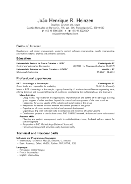
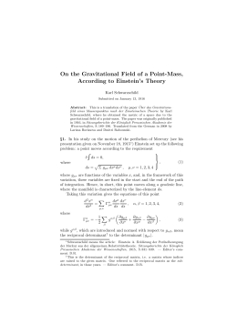
THE MINIMUM DELTA-V LAMBERT'S PROBLEM
Antonio Fernando Bertachini de Almeida Prado
Instituto Nacional de Pesquisas Espaciais São José dos Campos - SP - 12227-010 - Brazil
Phone (123)41-8977 E. 256 - Fax (123)21-8743 E-mail: [email protected]
Roger A. Broucke
Depto. Aerospace Eng. - Eng. Mechanics, Univ. ofTexas,
Austin-TX-78712-1085-USA.
Phone (512)471-4255 - Fax (512)471-3788 E-mai!: [email protected]
RESUMO. Este trabalho tem por objetivo formular e resolver
uma nova variante do conhecido "Problema de Lambert", um
dos mais importantes e discutidos tópicos em mecânica
celeste. A idéia é substituir a exigência de que a transferência
seja completada num tempo dado (problema original) pela
exigência de que o consumo de combustível envolvido nessa
manobra seja mínimo. Esse problema é resolvido através do
desenvolvimento de equações analíticas para as componentes
do impulso aplicado e teoria de rninirnização de funções. A
seguir, são feitas simulações para a comparação entre os
resultados obtidos por essa teoria e resultados disponíveis na
literatura. Esses resultados podem ser facilmente estendidos
para o estudo de uma transferência bi-impulsiva entre duas
órbitas Keplerianas coplanares com mínimo consumo de
combustível.
ABSTRACT. This paper formulates and solves a new version
of the well-known "Lambert's Problem," one of the most
important topics in celestial mechanics. The idea is to replace
the requirement that the transfer must be completed in a given
time (original problem) by the requirement that the fuel
expenditure involved in this transfer must be rninimum. This
problem is solved by developing analytical equations for the
components of the impulse applied and theory of rninirnization
of functions. Next, simulations are made to compare the
results obtained from this theory with results available in the
literature. Those results are easily extended to the study of biimpulsive transfers between two Keplerian and coplanar orbits
with rninimum expenditure of fuel.
Artigo Submetido em 10-10-94
l ' revisão 19·12-95; 2' revisão 12-03-95
Aceito sob recomendação do Ed. Cons. Prol. I)r. Rafael S. Mendes
84
SBA Controle & Automação I Vol. 7 nO 2 I maio a agosto 1996
1. INTRODUCTION
The original Lambert's problem is one of the most important
and popular topics in celestial mechanics. Several important
authors worked on it, trying to find better ways to solve the
numerical difficulties involved (Breakwell et alii 1961; Battin,
1965 and 1968; Lancaster et alii 1966; Lancaster &
Blanchard, 1969; Herrick, 1971; Prussing, 1979; Sun & Vinh,
1983; Taff & Randall, 1985; Gooding, 1990). It can be defined
as: "A Keplerian orbit, about a given gravitational center of
force is to be found connecting two given points (P I and P2) in
a given time Llt".
This paper formulates and proposes several forms to solve a
problem that is related to the Lambert's problem. This new
formulation is a little bit different from the original one, but it
also has many important applications. This new problem is
called "Minimum Delta-V Lambert's Problem" and it is
formulated as follows: "A Keplerian orbit, about a given
gravitational center of force is to be found connectin lY two
given points (P I that belongs to an initial orbit and P'"2 that
belongs to a final orbit), such that the LlV for the transfer is
rninimum".
To solve this problem, the analytical expressions for the total
increment of the velocity required LlV (as a function of only
one independent variable) and for its first derivative with
respect to this variable are obtained. Then, a numerical
scheme to get the root of the first derivative and the numeric
value of the LlV at this point is used. From this information it
is possible to get all the other parameters involved, like the
components of the impulses, their locations, etc. This research
is closely connected to the search for a rninimum two-impulse
transfer between two given coplanar orbits in the approach
hat is used in Prado (1993) and Broucke & Prado (1993). The
:mly difference is that the initial and final points of the
transfer are now fixed.
2. DEFINITION OF THE PROBLEM
Suppose that there is a spacecraft in a Keplerian orbit that is
called 0 0 (the initial orbit). It is desired to transfer this
spacecraft to a final Keplerian orbit 02, that is coplanar with
lhe orbit 00. To perform this transfer, we start at the point P I
(rI> aI)' where an impulse with magnitude LlV I that has an
angle <1>1 with the local transverse direction is applied. The
transfer orbit crosses the final orbit at the point P2 (r2, a2),
where an impulse with magnitude LlV 2 making an angle <1>2
with the local transverse direction is applied. To define the
basic problem (the "Minimum Delta-V Lambert's Problem"), it
is necessary to specify the true anomaly (aI) of the departure
point in the orbit 0 0 (point P I ) and the true anomaly (a 2) of
the point of arrival in the orbit O2 (point P2). With these two
values given and all the Keplerian elements of both orbits
known, it is possible to determine both radius vectors ~ and
r2 at the beginning and at the end of the transfer. Then the
problem is to find which transfer orbit connecting these two
vectors and using only two impulses is the one that requires
the minimum LlV for the maneuver. This problem is what is
defined here as the "Minimum LlV Lambert's Problem". The
sketch of the transfer and the variables used are shown in Fig.
1.
D = ~;
h =eSin(ro)
(1)
where 1.1 is the gravitational parameter of the central body; C is
the angular momentum of the orbit, e is the eccentricity and ro
is the argument of the periapse. The subscripts "O" for the
initial orbit, "1" for the transfer orbit and "2" for the final orbit
are also used. In those variables, the expressions for the radial
(subscript r) and transverse (subscript t) components of the
two impulses are:
LlVtl = DI -Do + (Dlk l -Doko)Cos(a l )+
(Dlh l
-
(3)
Doh o)Sin(a l )
(5)
The problem now is to find the transfer orbit that minimizes
the total LlV and that satisfies the two following constraints
equations, expressing the fact that the orbits intersect:
gl =
Using basic equations from the two-body celestial mechanics,
it is possible to write an analytical expression for the total LlV
(= LlV I + LlV2) required for this maneuver. To specify each of
the three orbits involved in the problem, the elements D, h and
k are used. They are defined by the following equations:
k = eCos(ro);
D~(I+koCos(al)+hoSin(al))­
Df (1 + k lcos(a l )+ hSin(a l )) =O
(6)
l
x
Final
Orbit
Fig. 1 - Geometry of the "Minimum LlV Lambert' s Problem".
SBA Controle & Automação IVo\. 7 nO 2 I maio a agosto 1996
85
gl
= Di(I+kzCos(Sl)+h1Sin(Sz))-
(7)
Df (1 + k jcos(sz)+ hjSin(Sz ))= O
.
.
Vij in the varlable D j. The expresslOns for
The problem is reduced to the one of finding the value of D j
that . gives the minimum value for the expression
~V = ~Vr~ + vti + JVr~ + Vt~
where i = r,t; j = 1,2 and the word "Direct" stands for the part
of the derivative that comes from the explicit dependence of ~
dk
and
j
d(~~j)
- - - can be obtained from the equations (2) to (5) and the
dh j
.
dk
oDj
j
expressions for -;-- and
3. USING THE CHAIN RULE FOR THE
DERIVATIVES
ah
j
aD
can be obtained from the
j
equations (8) to (9).
In this approach (and in the next one), the constraints (6) and
(7) are used to solve this system for two of our variables,
making the equation for the ~V a function of only one
independent variable. The system formed by these two
equations is symmetric and linear in the variables h j and kj, so
the system is solved for these two variables. The results are the
equations (8) and (9).
kl = -Csc(e l
d(~~j)
-e2{((~~ )1+koCOs(el)+hoSin(el))-I]sin(e2)-'"
-((~nl +k,eo,(e, )+h,Sin(e, ))-I}in(e,)]
With all those equations available, a numerical algorithm can
be built to iterate in the variable Dj to find the unique real root
a(~V)
a(~V)
of the equation - - = O. To obtain the value of -:..-- for
aD
dD j
a given Dj, necessary for the iteration process required, the
following steps can be used:
j
i) Evaluate k j and h j from equations (8) and (9) for the given
Dj ;
ii) With Dj, h j and k j the equations (2) to (5) are used to
evaluate
(8)
and
~Vrj, ~Vt1, ~Vr2' ~Vt2, ~Vj (~~Vr~ +~Vti
)
~V2 (J~Vr~ +~Vt~ );
iii) With all those quantities known, it is possible to evaluate
h = -csc(e1 -e2 { (
J
d(~ jj)
(~~ )t + k2Cos(e2)+~Sin(e2))-1 ]cos(eJ-...
a(~ !i)
and
ah
dk j
(obtained from equations (2) to
j
(5)) and equation (10) to finally obtain
-((~nl +koCo,(e, )+ hoSin(e, ))-1]co,(e,)]
d(~V)
aD
given Dj.
(9)
Now that the ~V is a function of only one variable (D j),
elementary calculus can be used to find its minimum. All that
has to be done is to search for the root of the expression
d(~V)
- - = O. From the definition of ~V it is possible to write:
dD j
4. SOLVING THE EQUATION
a(~v) =0
aD
j
At this point, it is important to remark that the function
a(~v)
dD j
is very sensitive to small variations in Dj, specially
100
SO
(lO)
60
40
Now, the chain rule for derivatives is applied to obtain
expressions
for
the
quantities
d(~Vrj). d(~Vt1). d(~Vrl). d(~Vt2)
A
general
dDj
dDj
dD j
dDj
expression for them is:
1.5S
1. 61
1.59
1. 62
4000
2000
1. 596 1.59S
1.6p2 1.604 1.606 1.60S
-2000
(lI)
-4000
Fig. 2 - ~V and its Derivative as a Function of D j
86
for the
j
SBA Controle & Automação I Vol. 7 n° 2 I maio a agosto 1996
,hen dose to the real roat. Its curve is almost a straight line
vith a slope that goes to infinity when 8 2 - 8] goes to 180°.
·ig. 2 shows the detail for a transfer where 82 - 8] = 3.14.
'rom that figure it is easy to see that this fact comes fiom the
harpness of the curve !1V x DI> when dose to the minimum.
[bis characteristic is particular for the set of variables used
md it is not a physical problem. If another independent
[ariable is used, like the argument of the periapse of the
ransfer orbit, the curve for the !1V x D] has a much less sharp
ninimum and, in consequence, its derivative has no big
umps.
Those equations alIow the calculation of the expression for
a(!1V)
- - - , that is given by expression (10). The partial
aD]
derivatives involved are given by:
[bis behavior makes numerical methods to find the roat based
)fi derivatives (like the popular Newton-Raphson) inadequate.
:n this research, the method of dividing the interval in two
)arts in each iteration shows to be adequate, although not fast
n convergence.
5. CALCULATING
~V(D1)
EXPLlCITLY
(17)
!\nother similar way to solve this problem is to use the
~uations for h] and k] (equations (8) and (9)) to find the
~uivalent of the equations (2) to (5) as a function of D] only.
!\fter some algebraic manipulations the folIowing expressions
:tunctions of D] only) can be obtainecl:
!1Vr ] = -
a(!1V,2) =
aD]
Csc(8] -82)[ (2
2)2 Dl +Do ...
2D]2
"-2(DJ2 + D]:)Cos(8] -8 2)-D]:k2Cos(8] - 28 2 }+...
"+(2D5ko - D]:kz)Cos(8])+ D]:h2Sin(8] - 28 2 }+···
Csc(8] -82) [ (2
2\,
2D
2 D] -D2 r-...
]
...+(2D5ho -
.. .+2(D5 - Df )cos(8] -82 )+",
Di hz )Sin(8])
]
(18)
...+(D5 k o -DOD]ko)cos(28] -82 )+",
.. .+(D5 k O+ DOD] k O- 2Di k 2 )Cos{8 2)+...
...+(D;ho - DoWzo )sin(2e e2 )+...
...+(D;ho + DoDiho- 2Di~)sin(e2) ]
l -
(12)
Now, the same technique of dividing the interval in two parts
in each iteration is used, to find the root of the equation (10).
6. USING LAGRANGE MULTIPLlERS
(13)
An elegant method to skip the algebraic work to solve
equations (6) and (7) for hl and kl is to introduce two
Lagrange multipliers /1.1 and 1-2. This is done by defining a
new function to be minimized, given by the expression:
(20)
...+(Di k 2 -D]D2k 2 )cos(8] -282 )+",
...+(Di k 2 +D]D2k 2 - 2D5ko)cOs{8])+...
...+(DJD2h2 -D]:h2 )Sin(8]-28 2}+...
(14)
...+(D]:h2 + DP2 h2 - 2D5ho)sin(8]) ]
!1Vt2
= ~2
J
[(D] - D2
Xl + k 2Cos(82 )+h2Sin(82))]
where gl and g2 are given by the equations (6) and (7).
Then, using the standard theory for Lagrange multipliers, the
five equations in the five unknowns Dl, hl, kl, 1-1, 1-2 that
have to be satisfied are obtained by treating alI the variables as
independent of the others. The equations are:
l[(
YL
__
aD] - !1V]
(15)
2
2)
D] -Do -DOhOh] +D]h] -DOkOk] +D]k] +
.. .+(2D J k] - DOk J - Doko )Cos(8])+...
SBA Controle & Automação 1 Vol. 7 nO 21 maio a agosto 1996
87
...+(2D]h] - DOh] - Doho)Sin(S])
l
(25)
After that, the system of equations (21) to (25) is solved by
numerical means. This solution gives all the information
required to consider the problem solved.
...+_1_. [ (D] - D2 - D2h/12 + D]h]2 - D2k]k 2 + D]kn+...
Mi
"+(2D]k]-D2k] -D2k2)cos(S2)+'"
...+ (2D]h] - D2h] - D2h2)s'in(S2)
J-..
The disadvantage of this approach is the increase in the
number of variables and equations from one to five. The
advantage is that the algebraic work to derive the previous
equations shown in this paper can be skipped.
(1 + k] Cos(S] )+h]Sin(S] )}-...
...-2À. 2D] (1 + k]COS(S2 )+h]Sin(S2 ))= O
(21)
7. RESULTS
...-2À.]D]
aI'
-a' =
h]
D
- ] , [D]k]-Doko+(D]-Do)Cos(s])]+
M]
+ DI. [D]kl -D2k2 +(D]-D2)CoS(S2)]-'"
d1
(22)
2
To test those equations, codes in standard FORTRAN are
developed to run some examples to get numerical results to
compare with the ones available in the literature. For this
purpose the initial and final orbit of the transfer are choose to
be the same ones chosen by Lawden (1991), when solving the
related problem of optimal two-impulse transfer. They are:
.. .-~DI2Sin(S])- ~D]2Sin(S2) = O
aa.~
Á]
1.
Do =
= D]. [D]hl
M·]
-
.J3; hO =O; kO = 1/3
Doho + (D] - Do)Sin(S])] +
D2
:]. [D]h] -D2h2 +(D] -D2),s'in(S2)] .-'"
2
~D]2COS(S])- ~D]2COS(S2) = O
(24)
360
o
45
= ..fi; h2 = 1/4; k2 = 0.4333
(23)
90
Then equation (10) is solved (by any of the forms showed in
this paper) to find D] and the respective d V for a given pair of
SI and S2' This process is repeated for values of SI and S2 in
the range O S; SI S; 360 and O S; S2 S; 360. Contour-plots are
made to show the behavior of the d V as a function of S] and
S2' Fig. 3 shows the results. Every point (Sj, S2) in that plot
is one particular case of the "Minimum Delta-V Lambert's
135 180 225 270 315, 360
360
315
315
270
270
225
225
180
180
135
135
90
90
45
45
O
O
O
45
90
135 180 225 270 315 360
Fig. 3 - Contour-Plot for d V as a Function of S] and S2'
88
SBA Controle & Automação I Vol. 7 nO 2 I maio a agosto 1996
61.00
185.18
61.06
61.13
61.19
61.25.
61.32
;
".
185.12
61.38
185.18
185.12
y o
"'>
c:i
185.05
184.99
184.93
.185.05
o
-~
-
184.99
184.93
184.86
184.80
61.00
184.86 .
61.06
61.13
61.19
61.25
61.32
184.80
61.38
Fig. 4 - Contour-Plot for t:N When 8 1 and 8 2 Are Close to the Absolute Minimum.
'roblem" and the ~V associated is the solution of this case.
lle whole picture is a collection of a large number of cases to
over all the possibilities. Fig. 4 is an amplification of the
egion dose to the absolute rninimum of ~V, as shown in
,awden (1991). From those plots it is possible to find the
egions (in 8 1 and 82) that give us a rninimum ~V orbit
ransfer between the two given orbits. If necessary, it is always
lossible to study in more detail a specific region, as done dose
::> the absolute rninimum in Fig. 4. This procedure has the
mportant practical applications of providing a good estimate
to be used as a good first guess) for the rninimum ~V transfer
letween the two orbits involved
S. CONCLUSIONS
REFERENCES
Battin, RR. (1965). Astronautical Guidance. McGraw-Hill,
New York, NY.
Battin, RR. (1968). A New Solution for Lambert's Problem.
Proccedings of the XIX lnternational Astronautical
Congress, Oxford, VoI. 2, pp. 131-150,.
Breakwell, lV., Gillespie, RW. & Ross, S. (1961).
Researches in Interplanetary Transfer. Journal of
American Rocket Society, VoI. 31, pp. 201-208.
Broucke, RA & Prado, AF.B.A (1993). Optimal N-Impulse
Transfer Between Coplanar Orbits. Paper AAS-93660. AAS/AIAA Astrodynarnics Meeting, Victoria,
Canadá.
['bis paper formulates and proposes a solution to the
Minimum Delta-V Lambert's Problem". This variant of the
•ambert's problem has the original requirement of completing
he transfer in a given time replaced by the new requirement
hat the transfer has a rninimum ~V. The analytical
:xpressions and numerical procedures to solve this problem
lfe derived in different ways. Contour-plots for a test case are
nade. It is also showed how to use this problem to solve the
)roblem of finding the rninimum ~V transfer orbit between
wo given coplanar orbits.
Gooding, RR. (1990). A Procedure for the Solution of
Lambert's
Orbital
Boundary-Value
Problem.
Celestial Mechanics, VoI. 48, pp. 145-165.
~cknowledgments:
Lancaster, E.R & Blanchard, RC. (1969). A Unified form of
Lambert's Theorem. Technical Note D-5368, NASA,
USA
Rerrick, S. (1971). Astrodynamics. Van Nostrand Reinhold,
London.
[be authors are grateful to CAPES (Federal Agency for Post}raduate Education - Brazil) and INPE (National Institute for
:>pace Research - Brazil) for supporting this research.
SBA Controle & Automação I Vol. 7 nO 2 I maio a agosto 1996
89
Lancaster, E.R, B1anchard, RC. & Devaney, RA. (1966). A
Note on Lambert's Theorem. Journal of Spacecraft
and Rockets, VoI. 3, pp. 1436-1438.
Lawden, D.F. (1991). Optima1 Transfers Between Coplanar
Elliptica1 Orbits. Journal of Guidance Contrai and
Dynamics, VoI. 15, No. 3, pp. 788-791.
Prado, A.F.B.A. (1993). Optima1 Transfer and Swing-By
Orbits in the Two- and Three-Body Prob1ems. Ph.D.
Dissertation, University of Texas, Austin, Texas,
USA.
Prussing, I.E. (1979). Geometrica1 Interpretation of the
Angles a and ~ in Lambert's Problem. Journal of
Guidance, Control, and Dynamics, VoI. 2, pp. 442443.
Sun, F.T. & Vinh, N.X. (1983). Lambertian Invariance and
Application to the Prob1em of Optimal Fixed-Time
Impulsive Orbital Transfer. Acta Astronautica, VoI.
10, pp. 319-330.
Taff, L.G. & Randall, P.M.S. (1985). Two Locations, Two
Times, and the Element Set. Celestial Mechanics,
VoI. 37, pp. 149-159.
90
SBA Controle & Automação I Vol. 7 nO 21 maio a agosto 1996