METHODOLOGIES
FOR THE
VEHICLES’ AGGREGATOR
PARTICIPATION
IN THE
OF AN
ELECTRIC
ELECTRICITY MARKETS
Ricardo Jorge Gomes de Sousa Bento Bessa
Thesis submitted to the Faculty of Engineering of University of
Porto in partial fulfillment of the requirements for the degree of
Doctor of Philosophy
Thesis Supervisor
Professor Manuel António Cerqueira da Costa Matos
Full Professor at the Department of Electrical and Computer Engineering
Faculty of Engineering, University of Porto
April 2013
”As we walked along the flatblock marina, I was calm on the outside, but thinking all the time - Now it was to be
Georgie the general, saying what we should do and what not to do, and Dim as his mindless greeding bulldog.
But suddenly, I viddied that thinking was for the gloopy ones, and that the oomny ones use like, inspiration and
what Bog sends. Now it was lovely music that came into my aid. There was a window open with the stereo on,
and I viddied right at once what to do.”
Alex, Clockwork Orange, 1971
Acknowledgments
The support of exceptional researchers, colleagues, friends and family was essential to conclude this work. Here, I will express a public word of appreciation and acknowledge their role
in this thesis.
This thesis was supervised by Professor Manuel Matos, Full Professor at the Faculty of Engineering of the University of Porto (FEUP), to who I am grateful for accepting this supervision. Professor Manuel Matos was much more than a supervisor, it was a true professor. His
guidance and advices allowed me to improve my scientific and personal competences, which
ultimately changed my viewpoints in different subjects.
The opportunity to work with Professors Peças Lopes and Vladimiro Miranda was also very
rewarding at different levels, and their teachings and enthusiasm influenced this thesis. I am
truly grateful to Professor Cláudio Monteiro since, on an early stage of my career, trusted in
me to work with him in different research projects. His friendship and advices were crucial to
follow this path and this thesis is also a result of his conviction in my capacities.
My former professors from the Faculty of Economics of the University of Porto, in particular
Professor João Gama, were responsible for making me think “out-of-the-box” and open to
multidisciplinary research.
In 2006, when I went to work at INESC Porto, the high quality of the human resources created
the perfect conditions to evolve at the scientific level. For me, it was a luck and a pleasure to
have true scientists as examples, such as Carlos Moreira, Luis Seca, André Madureira, Jorge
Pereira and Ricardo Ferreira. They were an inspiration to this thesis, and their support a valuable help. The opportunity to work with João Sousa and his friendship was essential for my
integration at INESC Porto and important for improving my programming skills. Furthermore,
the research work and the vision of Joel Soares and Pedro Almeida about the electric vehicles
topic, as well as their friendship and valuable discussions, was an important contribution to
this thesis. The help of Leonardo Bremermann was an essential support to combine the work
of the ANEMOS.plus project with this PhD thesis. The friendship and sense of humour during
critical (and non-critical) situations of Bernardo Silva were very gratifying during these years.
Finally, I cannot forget Célia Couto, Paula Castro and Rute Ferreira since their work made my
life much more easier during the PhD period.
At a personal level, I must dedicate a few paragraphs to acknowledge a group of persons that
made this work a reality.
First, thanks to my parents. It is not fair to work hard during their life in order to give a better
life to their children, and see both leave their home to graduate in another city. This thesis
and all my research work during these almost four years, is dedicated to them, for their effort,
for their support and for their love. To my sister Ana Rita, most of the time I was away and
unavailable, but she also played an important role. To my grandmother, who I know is very
proud of her grandson.
I also have a very good group of friends. I cannot mention all their names here because
the number of pages of this thesis would increase exponentially. I particularly acknowledge
Vanessa and António Pina, Joaquim Matos, Pedro Correia and Lourenço Moura since their
friendship, their words and advices in specific moments of my life were essential to complete
this path. The “mavericks” Pedro Costa and Tiago Azevedo were also essential to maintain the
equilibrium between the forces.
Finally, words are not enough to described the role and importance of my beloved Ana Pinto.
Her support and love during these years were the light during darkest times, the absolute
trust in my capacities was the fuel of this work, and her words were full of music and hope.
Definitely, this is also her thesis!
This work was supported by Fundação para a Ciência e a Tecnologia (FCT) de Portugal,
under PhD grant SFRH/BD/33738/2009 and by INESC TEC - Science and Technology.
Abstract
The Electric Vehicle (EV) is one element that contributes to a sustainable transport sector
since it helps reducing greenhouse gas (GHG) emissions and oil-dependency. It also establishes a connection between the transport and electric power sectors. In order to promote
a sustainable development, different stakeholders from the electric power sector are seeking
an increase of Renewable Energy Sources for Electricity (RES-E), complemented by a smart
grid infrastructure that enables a more active participation of the demand-side in the power
system operation.
The EV charging, if uncontrolled and during peak hours, could result in technical problems
at the distribution network level (e.g., branches congestion). However, direct-control of the
EV charging using the smart grid technology increases the demand-side flexibility which mitigates the technical problems and supports the integration of RES-E (e.g., by offering reserve
services). The existing electricity market rules do not allow bids from small loads and, in order
to decrease the communication requirements between the system operators and EV, a market
agent called aggregator can serve as an intermediary between a group of vehicle owners, electricity market, transmission and distribution system operators. Computational algorithms are
needed to make the smart grid architecture feasible.
Within this context, this PhD thesis explores the concept of an EV aggregator and contributes
with a set of computational tools that enable its active participation in the electricity market,
in particular the provision of secondary and balancing reserve services.
Firstly, a framework with optimization/forecasting models covering the majority of the electricity market sessions is defined. Then, day-ahead optimization models, based on forecasts
for the market prices and EV variables, are formulated to determine the bids for the electrical energy, secondary and balancing reserve market sessions. Operational management
algorithms, using information from the plugged-in EV and the accepted bids, are proposed to
coordinate EV charging during the operating day and comply with the market commitments
(e.g., avoid reserve shortage). The optimization models are evaluated in a test case with
synthetic EV time series and data from the Iberian electricity market.
The main contributions from this PhD thesis are: (a) day-ahead optimization models for
electrical energy, secondary and balancing reserve bids; (b) operational management algorithms that coordinate the EV individual charging and allow the provision of reserve without
compromising power system reliability; (c) estimation of the forecast errors impact on the
aggregator’s total cost and reserve shortage magnitude.
Resumo
O veículo elétrico (VE) é um elemento de uma solução global para o desenvolvimento sustentável do sector dos transportes, uma vez que permite reduzir as emissões de gases de efeito
de estufa e dependência do petróleo. Estabelece uma ligação com o sector elétrico, no qual
diferentes agentes procuram, em conjunto com o conceito de rede inteligente, aumentar a
contribuição de fontes de energia renovável para produção de eletricidade, promovendo um
desenvolvimento sustentável.
A integração de VE, com carregamento não-controlado, pode provocar problemas técnicos na
rede elétrica de distribuição. No entanto, o controlo do carregamento com base numa infraestrutura de comunicação bidirecional mitiga problemas técnicos e auxilia a integração de
geração de base renovável. De forma a reduzir os requisitos de comunicação para controlo
do carregamento, e dado que as atuais regras do mercado de eletricidade não permitem a
participação individual de pequenas cargas, é introduzido um novo agente de mercado chamado agregador de VE. Este agente serve de intermediário entre um grupo de VE, mercado
de eletricidade, operadores da rede de transporte e distribuição.
Neste contexto, esta tese de doutoramento explora o conceito de agregador e contribui com
um conjunto de algoritmos computacionais que permitem uma participação ativa do agregador no mercado de eletricidade, em particular no fornecimento de reserva secundária e de
balanço.
Numa primeira fase, é definida uma arquitetura que inclui modelos de previsão e otimização
para cada sessão do mercado. Em seguida, são formulados modelos de otimização, baseados
em previsões para o dia seguinte dos preços de mercado e consumo dos VE, com o objetivo
de otimizar as ofertas de energia elétrica e reserva. São igualmente propostos algoritmos
operacionais para coordenar o carregamento dos VE de forma a satisfazer os compromissos
do mercado elétrico durante o próprio dia e com base em informação de VE estacionados para
carregamento. Os modelos de otimização são testados num caso de estudo construído com
dados sintéticos do consumo de VE e dados reais do mercado Ibérico de eletricidade.
As principais contribuições desta tese são: (a) modelos de otimização para o dia seguinte
das propostas de compra de energia elétrica e venda de reserva secundária e de balanço; (b)
algoritmos operacionais que coordenam o carregamento individual dos VE, e permitem ao
agregador fornecer reserva sem comprometer a fiabilidade do sistema elétrico; (c) estimação
do impacto dos erros de previsão no custo total do agregador e na magnitude das situações
com reserva não-fornecida.
Contents
List of Figures
xvi
List of Tables
xx
List of Acronyms and Symbols
xxii
1 Introduction
1
1.1 General Context and Motivation . . . . . . . . . . . . . . . . . . . . . . . . . . . . . .
1
1.2 Objectives of the Thesis . . . . . . . . . . . . . . . . . . . . . . . . . . . . . . . . . . .
7
1.3 Structure of the Thesis . . . . . . . . . . . . . . . . . . . . . . . . . . . . . . . . . . . .
8
1.4 List of Publications . . . . . . . . . . . . . . . . . . . . . . . . . . . . . . . . . . . . . .
9
2 Background and State of the Art
11
2.1 Introduction . . . . . . . . . . . . . . . . . . . . . . . . . . . . . . . . . . . . . . . . . . 11
2.2 Background . . . . . . . . . . . . . . . . . . . . . . . . . . . . . . . . . . . . . . . . . . . 12
2.2.1 Power System Reserves . . . . . . . . . . . . . . . . . . . . . . . . . . . . . . . 12
2.2.2 Electricity Markets . . . . . . . . . . . . . . . . . . . . . . . . . . . . . . . . . . 16
2.2.3 Demand-side Active Participation . . . . . . . . . . . . . . . . . . . . . . . . . 21
2.3 Integration of EV into the Power System . . . . . . . . . . . . . . . . . . . . . . . . . 24
2.3.1 Early Studies . . . . . . . . . . . . . . . . . . . . . . . . . . . . . . . . . . . . . 24
2.3.2 Recent Studies . . . . . . . . . . . . . . . . . . . . . . . . . . . . . . . . . . . . 24
2.4 Economic and Technical Issues of EV in the Electricity Market . . . . . . . . . . . . 31
2.4.1 Peak and Base Power . . . . . . . . . . . . . . . . . . . . . . . . . . . . . . . . 31
2.4.2 Ancillary Services . . . . . . . . . . . . . . . . . . . . . . . . . . . . . . . . . . 33
2.4.3 Storage and RES-E . . . . . . . . . . . . . . . . . . . . . . . . . . . . . . . . . . 35
2.4.4 EV Aggregation Agent . . . . . . . . . . . . . . . . . . . . . . . . . . . . . . . . 35
2.4.5 Business Models for the Aggregator . . . . . . . . . . . . . . . . . . . . . . . 40
2.4.6 EV and Market Rules . . . . . . . . . . . . . . . . . . . . . . . . . . . . . . . . 44
xii
Contents
2.4.7 Summary and Remarks . . . . . . . . . . . . . . . . . . . . . . . . . . . . . . . 45
2.5 Smart Grid and Standardization . . . . . . . . . . . . . . . . . . . . . . . . . . . . . . 46
2.6 Algorithms for Supporting the EV Aggregator Business . . . . . . . . . . . . . . . . 50
2.6.1 Optimization Algorithms without Network Constraints . . . . . . . . . . . 50
2.6.2 Network Constrained Optimization Algorithms . . . . . . . . . . . . . . . . 59
2.6.3 Forecasting EV Variables . . . . . . . . . . . . . . . . . . . . . . . . . . . . . . 61
2.6.4 Battery Model for Optimization Algorithms . . . . . . . . . . . . . . . . . . . 62
2.6.5 Final Remarks . . . . . . . . . . . . . . . . . . . . . . . . . . . . . . . . . . . . . 63
3 EV Aggregator Model and Framework
65
3.1 Architecture . . . . . . . . . . . . . . . . . . . . . . . . . . . . . . . . . . . . . . . . . . 65
3.1.1 Interaction with EV Owner and Charging Point Manager . . . . . . . . . . 68
3.1.2 Interaction with TSO and DSO . . . . . . . . . . . . . . . . . . . . . . . . . . 72
3.1.3 Information Flows . . . . . . . . . . . . . . . . . . . . . . . . . . . . . . . . . . 74
3.1.4 Economic and Physical Flows . . . . . . . . . . . . . . . . . . . . . . . . . . . 76
3.2 Management Processes . . . . . . . . . . . . . . . . . . . . . . . . . . . . . . . . . . . . 79
3.3 Electricity Market Framework and Algorithms . . . . . . . . . . . . . . . . . . . . . 80
3.3.1 Short-term Horizon . . . . . . . . . . . . . . . . . . . . . . . . . . . . . . . . . 81
3.3.2 Very Short-term Horizon . . . . . . . . . . . . . . . . . . . . . . . . . . . . . . 83
3.3.3 Operational Management . . . . . . . . . . . . . . . . . . . . . . . . . . . . . 83
3.3.4 Market Settlement . . . . . . . . . . . . . . . . . . . . . . . . . . . . . . . . . . 84
3.4 Final Remarks . . . . . . . . . . . . . . . . . . . . . . . . . . . . . . . . . . . . . . . . . 84
4 Optimization Models for the Day-ahead Energy Market
87
4.1 Introduction . . . . . . . . . . . . . . . . . . . . . . . . . . . . . . . . . . . . . . . . . . 87
4.2 Global Approach . . . . . . . . . . . . . . . . . . . . . . . . . . . . . . . . . . . . . . . . 89
4.2.1 Representation of the EV Information . . . . . . . . . . . . . . . . . . . . . . 89
4.2.2 Advantages and Limitations . . . . . . . . . . . . . . . . . . . . . . . . . . . . 90
4.2.3 Formulation of the Optimization Problem . . . . . . . . . . . . . . . . . . . . 91
4.2.4 Forecasting Tasks . . . . . . . . . . . . . . . . . . . . . . . . . . . . . . . . . . . 94
4.3 Divided Approach . . . . . . . . . . . . . . . . . . . . . . . . . . . . . . . . . . . . . . . 96
4.3.1 Representation of the EV Information . . . . . . . . . . . . . . . . . . . . . . 96
4.3.2 Advantages and Limitations . . . . . . . . . . . . . . . . . . . . . . . . . . . . 96
4.3.3 Formulation of the Optimization Problem . . . . . . . . . . . . . . . . . . . . 97
4.3.4 Forecasting Tasks . . . . . . . . . . . . . . . . . . . . . . . . . . . . . . . . . . . 98
4.4 Operational Management Algorithm . . . . . . . . . . . . . . . . . . . . . . . . . . . 101
4.4.1 Formulation of the Optimization Problem . . . . . . . . . . . . . . . . . . . . 102
4.4.2 Forecasting the Imbalance Unit Costs . . . . . . . . . . . . . . . . . . . . . . 105
4.5 Test Case Description . . . . . . . . . . . . . . . . . . . . . . . . . . . . . . . . . . . . . 105
xiii
Contents
4.5.1 EV Synthetic Time Series . . . . . . . . . . . . . . . . . . . . . . . . . . . . . . 106
4.5.2 Electricity Market . . . . . . . . . . . . . . . . . . . . . . . . . . . . . . . . . . 107
4.5.3 Participation in the Electricity Market . . . . . . . . . . . . . . . . . . . . . . 108
4.5.4 Forecasting Models . . . . . . . . . . . . . . . . . . . . . . . . . . . . . . . . . 110
4.5.5 Sampling Process for Evaluation . . . . . . . . . . . . . . . . . . . . . . . . . 112
4.6 Comparison Between Global and Divided Optimization Models . . . . . . . . . . . 113
4.6.1 Illustrative Example of the Optimization Models Output and Results . . . 113
4.6.2 Comparison of the Deviations Between Accepted Bid and Actual Charging Values . . . . . . . . . . . . . . . . . . . . . . . . . . . . . . . . . . . . . . . 115
4.6.3 Comparison of Costs from Participating in the Electricity Market . . . . . 117
4.7 Sensitivity Analysis of the Global Approach . . . . . . . . . . . . . . . . . . . . . . . 122
4.8 Performance of the Operational Management Algorithm . . . . . . . . . . . . . . . 125
4.8.1 Comparison with State of the Art Operational Algorithms . . . . . . . . . . 125
4.8.2 The Impact of Very Short-term Forecasts . . . . . . . . . . . . . . . . . . . . 126
4.9 Discussion . . . . . . . . . . . . . . . . . . . . . . . . . . . . . . . . . . . . . . . . . . . 128
5 Optimization Models for the Secondary Reserve Market
131
5.1 Introduction . . . . . . . . . . . . . . . . . . . . . . . . . . . . . . . . . . . . . . . . . . 131
5.2 Problem Description . . . . . . . . . . . . . . . . . . . . . . . . . . . . . . . . . . . . . 132
5.2.1 Participation in the Electricity Market . . . . . . . . . . . . . . . . . . . . . . 132
5.2.2 Characteristics of the Secondary Reserve . . . . . . . . . . . . . . . . . . . . 135
5.3 Day-ahead Energy and Reserve Optimization . . . . . . . . . . . . . . . . . . . . . . 140
5.4 Operational Management Algorithm . . . . . . . . . . . . . . . . . . . . . . . . . . . 149
5.4.1 EV Fleet Operating Point and Calculation of the Available Reserve . . . . 150
5.4.2 Operational Management . . . . . . . . . . . . . . . . . . . . . . . . . . . . . 156
5.5 Market Settlement . . . . . . . . . . . . . . . . . . . . . . . . . . . . . . . . . . . . . . 161
5.6 Test Case Results . . . . . . . . . . . . . . . . . . . . . . . . . . . . . . . . . . . . . . . 163
5.6.1 Sampling Process . . . . . . . . . . . . . . . . . . . . . . . . . . . . . . . . . . . 164
5.6.2 Aggregator’s Viewpoint: Total Cost . . . . . . . . . . . . . . . . . . . . . . . . 164
5.6.3 TSO’s Viewpoint: Reserve Shortage . . . . . . . . . . . . . . . . . . . . . . . 168
5.6.4 Different Quality of the EV Variables Forecasts . . . . . . . . . . . . . . . . . 175
5.7 Final Remarks . . . . . . . . . . . . . . . . . . . . . . . . . . . . . . . . . . . . . . . . . 178
6 Optimization Models for the Balancing Reserve Market
181
6.1 Introduction . . . . . . . . . . . . . . . . . . . . . . . . . . . . . . . . . . . . . . . . . . 181
6.2 Problem Description . . . . . . . . . . . . . . . . . . . . . . . . . . . . . . . . . . . . . 182
6.2.1 Characteristics of the Balancing Reserve . . . . . . . . . . . . . . . . . . . . 182
6.2.2 Participation in the Electricity Market . . . . . . . . . . . . . . . . . . . . . . 185
6.3 Day-Ahead Energy and Reserve Optimization . . . . . . . . . . . . . . . . . . . . . . 187
xiv
Contents
6.3.1 Input Variables and Forecasts . . . . . . . . . . . . . . . . . . . . . . . . . . . 187
6.3.2 Formulation of the Optimization Problem . . . . . . . . . . . . . . . . . . . . 190
6.4 Operational Management Algorithms . . . . . . . . . . . . . . . . . . . . . . . . . . . 193
6.4.1 Operational Management for Day-Ahead Reserve Bids . . . . . . . . . . . . 193
6.4.2 Operational Management for Hour-Ahead Reserve Bids . . . . . . . . . . . 195
6.5 Market Settlement . . . . . . . . . . . . . . . . . . . . . . . . . . . . . . . . . . . . . . 202
6.6 Test Case Results . . . . . . . . . . . . . . . . . . . . . . . . . . . . . . . . . . . . . . . 204
6.6.1 Sampling Process . . . . . . . . . . . . . . . . . . . . . . . . . . . . . . . . . . . 204
6.6.2 Aggregator’s Viewpoint: Total Cost . . . . . . . . . . . . . . . . . . . . . . . . 205
6.6.3 TSO’s Viewpoint: Reserve Shortage . . . . . . . . . . . . . . . . . . . . . . . 208
6.6.4 Impact of the Reserve Direction Forecast . . . . . . . . . . . . . . . . . . . . 210
6.6.5 Different Quality of the EV Variables Forecasts . . . . . . . . . . . . . . . . . 215
6.7 Final Remarks . . . . . . . . . . . . . . . . . . . . . . . . . . . . . . . . . . . . . . . . . 216
7 General Conclusions and Future Work
7.1
219
Contributions and Main Findings . . . . . . . . . . . . . . . . . . . . . . . . . . . . . 219
7.1.1 Contributions . . . . . . . . . . . . . . . . . . . . . . . . . . . . . . . . . . . . . 219
7.1.2 Main Findings . . . . . . . . . . . . . . . . . . . . . . . . . . . . . . . . . . . . . 220
7.2 Perspectives for Future Work . . . . . . . . . . . . . . . . . . . . . . . . . . . . . . . . 223
Bibliography
227
A Statistical Analyses of the Test Case Data
251
A.1 Synthetic EV Time Series . . . . . . . . . . . . . . . . . . . . . . . . . . . . . . . . . . 251
A.1.1 Individual EV . . . . . . . . . . . . . . . . . . . . . . . . . . . . . . . . . . . . . 251
A.1.2 Aggregated EV . . . . . . . . . . . . . . . . . . . . . . . . . . . . . . . . . . . . 257
A.2 Energy and Reserve Prices . . . . . . . . . . . . . . . . . . . . . . . . . . . . . . . . . . 262
B Evaluation of the Forecast Performance
267
B.1 Aggregated EV Variables . . . . . . . . . . . . . . . . . . . . . . . . . . . . . . . . . . . 267
B.2 Individual EV Variables . . . . . . . . . . . . . . . . . . . . . . . . . . . . . . . . . . . . 268
B.2.1 Forecast Error of the Changed Forecasts . . . . . . . . . . . . . . . . . . . . . 271
B.3 Market Prices . . . . . . . . . . . . . . . . . . . . . . . . . . . . . . . . . . . . . . . . . . 273
B.4 Reserve Direction . . . . . . . . . . . . . . . . . . . . . . . . . . . . . . . . . . . . . . . 274
C State of the Art Operational Algorithms
277
C.1 Priority-based Algorithm . . . . . . . . . . . . . . . . . . . . . . . . . . . . . . . . . . . 277
C.2 Price-ranking-based Algorithm . . . . . . . . . . . . . . . . . . . . . . . . . . . . . . . 278
xv
List of Figures
1.1 Final energy savings of the European transport sector and forecasted number
of electric vehicles . . . . . . . . . . . . . . . . . . . . . . . . . . . . . . . . . . . . . . .
3
1.2 Life cycle GHG emissions from vehicles shown as a function of the life cycle
GHG intensity of electricity generation . . . . . . . . . . . . . . . . . . . . . . . . . .
4
2.1 Frequency control scheme and actions of the ENTSO-E operational handbook . . 14
2.2 Response time and duration of different reserve categories in the USA . . . . . . 15
2.3 Structure of the electricity market . . . . . . . . . . . . . . . . . . . . . . . . . . . . . 16
2.4 Illustrative example of an EV providing regulation up and down . . . . . . . . . . 25
2.5 A test on providing two hours of secondary reserve . . . . . . . . . . . . . . . . . . 34
2.6 Technical management and market operation framework for EV integration . . . 37
2.7 “Package deal” business model . . . . . . . . . . . . . . . . . . . . . . . . . . . . . . . 42
2.8 Standards used in the EDISON project . . . . . . . . . . . . . . . . . . . . . . . . . . 49
3.1 EV aggregator architecture . . . . . . . . . . . . . . . . . . . . . . . . . . . . . . . . . 68
3.2 Components of public (or semi-public) and fast charging stations for AggregatorEV-CPM interaction. . . . . . . . . . . . . . . . . . . . . . . . . . . . . . . . . . . . . . 70
3.3 Components of a residential or office charging station . . . . . . . . . . . . . . . . 71
3.4 Information flows between aggregator, DSO/TSO, EV and CPM . . . . . . . . . . . 76
3.5 Economic and physical flows between aggregator, DSO/TSO and EV driver . . . 77
3.6 Electricity market framework and algorithms for the EV aggregator . . . . . . . . 81
3.7 EV variables: charging requirement and availability . . . . . . . . . . . . . . . . . . 82
4.1 Global and divided approaches for short-term management . . . . . . . . . . . . . 88
4.2 Seasonal plots for EV availability of one and 1500 EV . . . . . . . . . . . . . . . . . 90
4.3 Total charging requirement forecast and realized value . . . . . . . . . . . . . . . . 95
4.4 Availability forecast and realized value of one EV . . . . . . . . . . . . . . . . . . . 101
4.5 Diagram with the sequence of tasks for participating in the electricity market . . 108
xvi
LIST OF FIGURES
4.6 Diagram with the temporal horizons of the forecast and optimization models . . 109
4.7 Accepted bids of the global and divided approaches for one illustrative day . . . 114
4.8 Accepted bids and actual charging (from the operational algorithm) for one
illustrative day . . . . . . . . . . . . . . . . . . . . . . . . . . . . . . . . . . . . . . . . . 115
4.9 MAPD of the divided approach with forecasted information for fleets A and B . . 117
4.10 MAPD of the global approach (for fleets A and B) with forecasted and realized
values of the EV variables as input . . . . . . . . . . . . . . . . . . . . . . . . . . . . . 118
4.11 DBIAS of the global approach (for fleets A and B) with forecasted and realized
values of the EV variables as input . . . . . . . . . . . . . . . . . . . . . . . . . . . . . 119
4.12 Total cost increase between the divided approach with forecasted and realized
values used as input in the day-ahead optimization . . . . . . . . . . . . . . . . . . 119
4.13 Total cost increase between the global approach with forecasted and realized
values used as input in the day-ahead optimization . . . . . . . . . . . . . . . . . . 120
4.14 Costs reduction of the divided and global approach in fleet A compared to the
inflexible EV load approach . . . . . . . . . . . . . . . . . . . . . . . . . . . . . . . . . 120
4.15 Costs reduction of the divided and global approach in fleet B compared to the
inflexible EV load approach . . . . . . . . . . . . . . . . . . . . . . . . . . . . . . . . . 121
4.16 β against MAPD for different aggregation sizes and fleet A . . . . . . . . . . . . . 123
4.17 β against MAPD of different aggregation sizes and fleet B . . . . . . . . . . . . . . 123
4.18 The impact of β in the components of the total cost for fleet A . . . . . . . . . . . 124
4.19 The impact of β in the components of the total cost for fleet B . . . . . . . . . . . 124
4.20 Aggregation size against MAPD for fleets A and B obtained with four different
operational algorithms . . . . . . . . . . . . . . . . . . . . . . . . . . . . . . . . . . . . 126
4.21 Surplus and shortage costs for fleets A and B obtained with three different
operational algorithms . . . . . . . . . . . . . . . . . . . . . . . . . . . . . . . . . . . . 127
5.1 Market clearing of the secondary reserve bids . . . . . . . . . . . . . . . . . . . . . . 133
5.2 Sequence of tasks for participating in the day-ahead energy and secondary reserve markets . . . . . . . . . . . . . . . . . . . . . . . . . . . . . . . . . . . . . . . . . 134
5.3 Secondary reserve . . . . . . . . . . . . . . . . . . . . . . . . . . . . . . . . . . . . . . . 135
5.4 PJM AGC regulation signal for 6 hours . . . . . . . . . . . . . . . . . . . . . . . . . . 136
5.5 Histograms for the number of equivalent minutes of the upward secondary
reserve of a hydro and thermal power plants in Portugal for the year 2011 . . . . 137
5.6 Histograms of the secondary reserve in Portugal and PJM. . . . . . . . . . . . . . . 138
5.7 Autocorrelation plots of the secondary reserve in Portugal and PJM. . . . . . . . . 138
5.8 Day-ahead forecast of the secondary reserve capacity price . . . . . . . . . . . . . 141
5.9 One step-ahead forecast of the upward tertiary reserve price in Portugal . . . . . 142
5.10 POP, upward and downward reserve power of one EV . . . . . . . . . . . . . . . . . 142
xvii
LIST OF FIGURES
5.11 Output of the day-ahead optimization for one illustrative day of the test case
(fleet A) . . . . . . . . . . . . . . . . . . . . . . . . . . . . . . . . . . . . . . . . . . . . . 147
5.12 Output of the day-ahead optimization for one illustrative day of the test case
(fleet B) . . . . . . . . . . . . . . . . . . . . . . . . . . . . . . . . . . . . . . . . . . . . . 149
5.13 Outputs of the day-ahead optimization for energy and secondary reserve bids . . 150
5.14 Increase in secondary reserve by starting the non-adjustable generator M3 as
tertiary reserve . . . . . . . . . . . . . . . . . . . . . . . . . . . . . . . . . . . . . . . . . 152
5.15 Variables required to redefine the operating point . . . . . . . . . . . . . . . . . . . 153
5.16 Illustrative examples for the calculation of the redefined operating point . . . . . 156
5.17 Illustrative example of the operational management algorithm output for secondary reserve and fleet A . . . . . . . . . . . . . . . . . . . . . . . . . . . . . . . . . . 159
5.18 Illustrative example of the operational management algorithm output for secondary reserve and fleet B . . . . . . . . . . . . . . . . . . . . . . . . . . . . . . . . . . 160
5.19 Total cost reduction in fleets A and B from selling secondary reserve . . . . . . . . 165
5.20 Reduction in the total cost for both fleets and with different sets of available
information . . . . . . . . . . . . . . . . . . . . . . . . . . . . . . . . . . . . . . . . . . . 167
5.21 pCRPS and pICRPS for upward and downward reserve directions . . . . . . . . . 171
5.22 pCRPS and pICRPS for upward reserve as a function of two different tolerances
for the target SoC . . . . . . . . . . . . . . . . . . . . . . . . . . . . . . . . . . . . . . . 172
5.23 pRNS and pIRNS of upward and downward reserve in fleets A and B . . . . . . . 174
5.24 pCRPS and pRNS of upward and downward reserve in fleets A and B for different qualities of charging requirement and availability forecast (with a ratio
between upward and downward reserve bids) . . . . . . . . . . . . . . . . . . . . . 177
5.25 pCRPS and pRNS of upward and downward reserve in fleets A and B for different qualities of charging requirement and availability forecast (with separated
upward and downward reserve bids) . . . . . . . . . . . . . . . . . . . . . . . . . . . 178
6.1 Balancing reserve . . . . . . . . . . . . . . . . . . . . . . . . . . . . . . . . . . . . . . . 183
6.2 Market clearing of the balancing reserve bids . . . . . . . . . . . . . . . . . . . . . . 186
6.3 Sequence of tasks for participating in the energy and balancing reserve market
sessions . . . . . . . . . . . . . . . . . . . . . . . . . . . . . . . . . . . . . . . . . . . . . 187
6.4 Autocorrelation diagrams of the binary variable that indicates if the secondary
and balancing reserve was dispatched in the upward direction . . . . . . . . . . . 188
6.5 Illustrative examples of the day-ahead energy and balancing reserve optimization192
6.6 Illustrative example of the day-ahead and hour-ahead operational management
algorithms output for balancing reserve . . . . . . . . . . . . . . . . . . . . . . . . . 201
6.7 Reduction in the total cost compared to optimizing only the energy bids . . . . . 206
6.8 Total cost reduction of three different sets of available information . . . . . . . . 207
6.9 Upward pRNS and pIRNS in fleets A and B . . . . . . . . . . . . . . . . . . . . . . . 209
xviii
LIST OF FIGURES
6.10 Upward and downward pRNS and pIRNS of fleets A and B, assuming that the
reserve is not fully dispatched during each time interval . . . . . . . . . . . . . . . 211
6.11 pRNS of upward and downward balancing reserve in fleets A and B for different
qualities of the charging requirement and availability forecast . . . . . . . . . . . 216
A.1 Availability daily pattern of each EV from fleet A divided by driver type . . . . . . 252
A.2 Frequency of arrivals and departures in each time intervals from three EV from
fleet A . . . . . . . . . . . . . . . . . . . . . . . . . . . . . . . . . . . . . . . . . . . . . . 253
A.3 Boxplots summarizing the average and maximum plugged-in time of fleet A . . . 254
A.4 Boxplots summarizing the average and maximum plugged-in time of fleet B . . . 254
A.5 Boxplots summarizing the average initial and target SoC of fleet A . . . . . . . . . 255
A.6 Boxplots summarizing the average initial and target SoC of fleet B . . . . . . . . . 255
A.7 Boxplots summarizing the average flexibility of each EV in fleets A and B . . . . . 256
A.8 Autocorrelation diagram of the availability time series of one EV of each type . . 258
A.9 Seasonal plot of the aggregated variables from fleet A . . . . . . . . . . . . . . . . 259
A.10 Seasonal plot of the aggregated variables from fleet B . . . . . . . . . . . . . . . . . 260
A.11 Autocorrelation diagram of the aggregated variables from fleet A . . . . . . . . . 261
A.12 Boxplots conditioned to the hour of the day for the market prices of year 2009 . 263
A.13 Boxplots conditioned to the hour of the day for the market prices of year 2010 . 264
A.14 Boxplots conditioned to the hour of the day for the market prices of year 2011 . 264
A.15 Autocorrelation plot of the energy and secondary reserve capacity prices for
year 2011 . . . . . . . . . . . . . . . . . . . . . . . . . . . . . . . . . . . . . . . . . . . . 265
B.1 Boxplot with the accuracy of the availability forecast for fleets A and B . . . . . . 269
B.2 Boxplot with the mMAPE for the charging requirement of fleets A and B . . . . . 270
B.3 Spearman correlation and mean absolute error of the prices forecasts . . . . . . . 273
B.4 Mean absolute error of the forecasts for the tertiary and secondary reserve
prices in Portugal . . . . . . . . . . . . . . . . . . . . . . . . . . . . . . . . . . . . . . . 274
xix
List of Tables
2.1 Economic value of different types of EV in the electricity market . . . . . . . . . . 45
4.1 Illustrative example of three EV with charging process controlled by the aggregator . . . . . . . . . . . . . . . . . . . . . . . . . . . . . . . . . . . . . . . . . . . . . . . 91
4.2 Illustrative example of the charging requirement distribution of three EV . . . . . 93
4.3 Parameters of the truncated Gaussian probability density function . . . . . . . . . 106
4.4 Three types of behavior regarding EV charging . . . . . . . . . . . . . . . . . . . . . 107
4.5 Total cost increase and deviations obtained from not including very short-term
forecasts in the operational algorithm . . . . . . . . . . . . . . . . . . . . . . . . . . 128
5.1 Secondary reserve bids from one EV plugged-in during four hours and net electrical energy that results from the reserve provision during the first two hours . 140
5.2 Set of charging solutions of an EV offering upward reserve power . . . . . . . . . 145
5.3 Example of a charging solution of an EV offering upward and downward reserve power . . . . . . . . . . . . . . . . . . . . . . . . . . . . . . . . . . . . . . . . . . 146
5.4 Total cost’s components of settlement scheme (a) for a test sample of fleet B . . 166
5.5 Percentage of upward and downward reserve power shortage . . . . . . . . . . . . 169
5.6 Standard deviation values used in the truncated Gaussian distributions for the
charging requirement and availability forecasts . . . . . . . . . . . . . . . . . . . . . 176
6.1 Illustrative example of the upward and downward balancing reserve dispatch
in Portugal . . . . . . . . . . . . . . . . . . . . . . . . . . . . . . . . . . . . . . . . . . . 185
6.2 Downward pRNS and pIRNS from fleets A and B . . . . . . . . . . . . . . . . . . . . 208
6.3 pRNS of the upward and downward balancing reserve and total cost increase
with different forecasts for the reserve direction . . . . . . . . . . . . . . . . . . . . 212
6.4 Total cost’s components for one test sample with different forecasts for the
reserve direction . . . . . . . . . . . . . . . . . . . . . . . . . . . . . . . . . . . . . . . . 214
xx
LIST OF TABLES
6.5 Standard deviation values used in the truncated Gaussian distributions for the
charging requirement and availability forecasts . . . . . . . . . . . . . . . . . . . . . 215
A.1 Summary statistics of the average ratio between charging requirement and battery size for all vehicles from fleet A . . . . . . . . . . . . . . . . . . . . . . . . . . . . 256
A.2 Summary statistics of the average ratio between charging requirement and battery size for all vehicles from fleet B . . . . . . . . . . . . . . . . . . . . . . . . . . . . 256
A.3 Summary statistics of aggregated EV variables of fleet A . . . . . . . . . . . . . . . 257
A.4 Summary statistics of aggregated EV variables of fleet B . . . . . . . . . . . . . . . 257
A.5 Summary statistics of day-ahead electrical energy price for years 2009, 2010
and 2011 in Portugal . . . . . . . . . . . . . . . . . . . . . . . . . . . . . . . . . . . . . 262
A.6 Summary statistics of upward tertiary reserve price for years 2009, 2010 and
2011 in Portugal . . . . . . . . . . . . . . . . . . . . . . . . . . . . . . . . . . . . . . . . 262
A.7 Summary statistics of downward tertiary reserve price for years 2009, 2010
and 2011 in Portugal . . . . . . . . . . . . . . . . . . . . . . . . . . . . . . . . . . . . . 262
A.8 Summary statistics of secondary reserve capacity price for years 2009, 2010
and 2011 in Portugal . . . . . . . . . . . . . . . . . . . . . . . . . . . . . . . . . . . . . 263
B.1 Forecasting performance for the EV aggregated variables for fleets A and B . . . 268
B.2 mMAPE of the aggregated availability and charging requirement forecast for
fleets A and B with 1500 EV . . . . . . . . . . . . . . . . . . . . . . . . . . . . . . . . . 270
B.3 mPBIAS of the aggregated availability and charging requirement forecast for
fleets A and B with 1500 EV . . . . . . . . . . . . . . . . . . . . . . . . . . . . . . . . . 270
B.4 mMAPE and mPBIAS of the modified aggregated availability and charging requirement forecast for fleet A . . . . . . . . . . . . . . . . . . . . . . . . . . . . . . . . 272
B.5 mMAPE and mPBIAS of the modified aggregated availability and charging requirement forecast for fleet B . . . . . . . . . . . . . . . . . . . . . . . . . . . . . . . . 272
B.6 Accuracy and Area Under the ROC Curve (AUC) of the day-ahead forecasts for
the balancing reserve direction in Portugal . . . . . . . . . . . . . . . . . . . . . . . 275
B.7 Accuracy and Area Under the ROC Curve (AUC) of the hour-ahead forecasts for
the balancing reserve direction in Portugal . . . . . . . . . . . . . . . . . . . . . . . 275
B.8 Accuracy of four different basic (or heuristic) binary forecast models . . . . . . . 275
xxi
List of Acronyms and Symbols
Acronyms
AC
Alternate Current
ACE
Area Control Error
AGC
Automatic Generation Control
AIC
Akaike Information Criterion
AMI
Advanced Metering Infrastructure
BETTA
British Electricity Trading and Transmission Arrangements
BMS
Battery Management System
BPA
Bonneville Power Administration
CAISO
California Independent System Operator
CAMC
Central Autonomous Management Controller
CAU
Central Aggregation Unit
CD
Control Device
CPM
Charging Point Manager
CSP
Curtailment Service Providers
CVC
Clusters of Vehicle Controllers
DBIAS
Deviations Bias
DC
Direct Current
DLC
Direct Load Control
DMS
Distribution Management System
DR
Demand Response
xxii
Acronyms
DSO
Distribution System Operator
EDA
Estimation Distribution Algorithm
ENTSO-E
European Network of Transmission System Operators for Electricity
ERCOT
Electric Reliability Council of Texas
ERGO
Electric Recharge Grid Operator
ESP
Energy Service Providers
EV
Electric Vehicle
EVC
External Vehicle Charger
EVM
Electric Vehicle Meter
EVSE
Electric Vehicle Supply Equipment
FAN
Field Area Network
GHG
Greenhouse Gas
GLM
Generalized Linear Model
HAN
Home Area Network
HSL
High Sustained Limit
ICT
Information and Communications Technology
IEC
International Electrotechnical Commission
IP
Internet Protocol
ISO
ISO New England
ISO
Independent System Operator
LMP
Locational Marginal Price
LOLE
Loss of Load Expectation
LSL
Low Sustained Limit
MAE
Mean Absolute Error
MAPD
Mean Absolute Percentage value of the Deviations
MAPE
Mean Absolute Percentage Error
MG
MicroGrid
MGAU
MicroGrid Aggregation Unit
MGCC
MicroGrid Central Controller
xxiii
Acronyms
MISO
Midwest ISO
MMG
MultiMicroGrid
NERC
North American Electric Reliability Corporation
NYISO
New York ISO
OC
On-board Computer
OPF
Optimal Power Flow
OVC
On-board Vehicle Charger
PBIAS
Percentage Bias
pCRPS
Percentage of Constant Reserve Power Shortage
pICRPS
Percentage of Intervals with Constant Reserve
Power Shortage
pIRNS
Percentage of Intervals with Reserve Not Supplied
PJM
Pennsylvania-New Jersey-Maryland Interconnection
PLC
Power Line Communication
POP
Preferred Operating Point
pRNS
Percentage of Reserve Not Supplied
pRPS
Percentage of Reserve Power Shortage
RES-E
Renewable Energy Sources for Electricity
RNS
Reserve Not Supplied
RTO
Regional Transmission Organization
SAE
Society of Automotive Engineers
SEI
Solid Electrolyte Interphase
SoC
State of Charge
TCP
Transmission Control Protocol
TSO
Transmission System Operator
UCTE
Union for the Co-ordination of Transmission of
Electricity
V2G
Vehicle-to-Grid
xxiv
List of symbols
V2V
Vehicle-to-Vehicle
VC
Vehicle Controller
List of symbols
µ
Ratio between upward and downward secondary reserve power.
αt
Factor that relates the maximum charging
power with the percentage of satisfied charging
requirement.
β
Coefficient of the linear relation between the
maximum charging power and the percentage
of satisfied charging requirement.
∆ dk own
Variable for adjusting the initial downward reserve bids in time interval k.
∆t
Time step (length of the time interval) of time
interval t.
up
∆k
Variable for adjusting the initial upward reserve
bids in time interval k.
Dt
Seasonal index that takes a different value for
each day of the week.
E tbase
Baseline for the upward balancing reserve in
time interval t.
E tbid
Accepted energy bid in the day-ahead market
for time interval t.
E tcons
EkDA
E td own∗
Consumed electrical energy in time interval t.
Initial plan from the day-ahead optimization.
Dispatched downward balancing reserve in
time interval t.
ǫt
Unobservable error term (or disturbance).
Et
Optimized electrical energy for time interval t.
E t, j
Optimized electrical energy for charging the jth
EV in time interval t.
xxv
List of symbols
E t,∗ j
Electrical energy consumed by the jth EV in time
interval t.
up∗
Et
Dispatched upward balancing reserve in time
interval t
g
Smoothing spline.
H
Set of time intervals from the optimization horizon.
plug
Ĥ j
[i]
ith forecasted availability (or plugged-in) period
of the jth EV.
plug
Hj
[i]
ith availability (or plugged-in) period of the jth
EV.
ht
Seasonal index that takes a different value for
each hour of the day.
E x por t
It
Cross-border exported electrical energy during
time interval t.
I mpor t
It
Cross-border imported electrical energy during
time interval t.
Lj
Number of availability periods of the jth EV.
l
Maximum order of lagged variables.
λdt own
Number of equivalent minutes of dispatched
downward secondary reserve in interval t.
up
λt
Number of equivalent minutes of dispatched
upward secondary reserve in interval t.
ϕ
Convex loss function.
Mt
Total number of EV plugged-in at time interval
t.
Φ
Costs associated to reserve shortage.
φ
Regression model’s coefficients.
π−
t
+
πt
P̂tma x
Negative imbalance unit cost of time interval t.
Positive imbalance unit cost of time interval t.
Forecasted total maximum charging power in
time interval t.
xxvi
List of symbols
P̄tmax
0
Maximum, constant and feasible charging
power of the EV fleet in time interval t 0 .
P̄tmin
0
Minimum, constant and feasible charging
power of the EV fleet in time interval t 0 .
P jma x
Pt,d own
j
Maximum charging power of the jth EV.
Downward secondary reserve power of the jth
EV for time interval t.
up
Pt, j
Upward secondary reserve power of the jth EV
for time interval t.
shor t a g e
pt
sur plus
pt
Price for negative imbalances of time interval t.
Ψ
Costs associated to deviations between actual
Price for positive imbalances of time interval t.
charging and accepted bids.
p̂ t
Day-ahead energy price forecast for time interval t.
Pt′
0
Operating point (or actual preferred operating
point).
Pt′d own
0
′up
Pt 0
cap
p̂ t
p̂ dt own
Available downward secondary reserve power.
Available upward secondary reserve power.
Forecasted capacity price of secondary reserve.
Forecasted price for dispatched downward reserve.
P̄td own
Downward secondary reserve power that can
be sustained during interval t.
up
P̄t
Upward secondary reserve power that can be
sustained during interval t.
pt
Day-ahead energy price for time interval t.
up
p̂ t
upper
P̄t 0
Forecasted price for dispatched upward reserve.
Upper power limit that guarantees full availability of downward reserve power in time interval t 0 .
P̄tl ower
0
Lower power limit that guarantees full availability of upward reserve power in time interval
t0 .
γ
Penalization coefficient for secondary reserve
capacity shortage.
xxvii
List of symbols
ρ
Penalization coefficient for reserve not supplied
(electrical energy).
R̂ j,i
Forecasted charging requirement for the ith
availability period of the jth EV.
RN S td own
Downward reserve not supplied in time interval
t.
up
RN S t
Upward reserve not supplied in time interval t.
R̂ t
Forecasted total charging requirement for time
interval t.
R t 0 , j,i
Residual charging requirement for the ith availability period of the jth EV at beginning of time
instant t 0 .
R̂ Dt
Forecasted total charging requirement distribution for time interval t.
T
Time interval of the last plugged-in EV to depart.
t
Time interval.
t0
First time interval.
τ+
t
Binary variable for the upward balancing downward reserve direction.
τ−
t
Binary variable for the upward balancing upward reserve direction.
t f inal
Last time interval of the availability period.
t ini t ial
First time interval of the availability period.
vk
Slack variable.
wp t
Forecasted wind power penetration level.
y
Response variable from a regression model.
y t− j
jth lag of the response variable y.
xxviii
Chapter
1
Introduction
1.1 General Context and Motivation
Sustainable development is as much an economic necessity as it is an environmental and social
obligation. This term was introduced, in 1987, by the Brundtland Commission report as the
“development that meets the needs of the present without compromising the ability of future generations to meet their own needs” [1]. This concept provides guidelines for strategic
decision-making for planning human activities using a holistic approach that includes environmental, social and economic long-term goals. The electric power and transport sectors are
following these fundamental guidelines to construct their sustainable paths.
The sustainable path of the electric power system is mainly characterized by the following
actions [2][3]: increase energy efficiency in generation, transmission and distribution of electrical energy; high quality and security of supply; promotion of energy efficiency and saving
measures in final costumers combined with smart meters deployment; increase the share of
Renewable Energy Sources for Electricity (RES-E). The main goals/outcomes are greenhouse
gas (GHG) emissions reduction, primary energy dependency reduction, social and economic
development of regions/country (e.g., lower electricity prices, contribution from the RES-E
sector to increase employment rate).
In the transport sector, the term sustainable transport can be defined as “transportation that
does not endanger public health or ecosystems and meets mobility needs consistent with (a)
use of renewable resources at below their rates of regeneration and (b) use of non-renewable
resources at below the rates of development of renewable substitutes.” [4].
In the European Union (EU), the GHG emissions from the transport sector increased around
1
1.1. General Context and Motivation
36% since 1990, which degraded the environmental quality [5]. This sector, because of its oildependency, is responsible for around a quarter of EU GHG emissions, and the road transport
represents about one-fifth of the EU’s CO2 total emissions1 . Moreover, concerns such as the
dependency on oil supply [6] and a foreseen “end of cheap oil” during this century [7] have
motivated a wide range of policy and technological measures for the transport sector.
The European Commission (EC), in order to promote the use of energy from renewable resources, approved the Directive 2009/28/EC [8] that sets a mandatory target of 20% share
of energy from renewable sources in the Community’s gross final consumption of energy by
2020 and a mandatory 10% minimum target of energy from renewable sources in the transport sector. The target for the transport sector should be pursued with a mix between different
technological solutions (e.g., hybrid and battery electric vehicles, biofuels, hydrogen) [9] and
policies (e.g., including the transport sector in the EU Emissions Trading System, behavior
change programs, standards for fuel quality) [10]. The EC strategy consists in supporting the
market development of alternative fuels and investment in their infrastructure [9].
The Electric Vehicle (EV) is one element that helps to decarbonize the transport sector and
decrease its oil-dependency [11][12]. There are three main types of EV [13]: battery, hybrid
and fuel cell. The hybrid EV combines an internal combustion engine with batteries and
electric motor. The hybrid EV is divided into two groups: conventional vehicles that, for
instance, charge the battery using regenerative braking that converts the vehicle’s kinetic
energy into electrical energy; vehicles capable of plugging-in with the electric system to charge
and discharge the batteries. The fuel cell EV uses hydrogen to generate electricity that can be
used for driving or stored in batteries and can plug-in for discharging stored electrical energy.
Presently, plug-in EV are a niche in the global market. In [14], it is forecasted a decrease
to a third of conventional combustion vehicles sales by 2030, and an increase of the hybrid
EV (full hybrids 22%, mild hybrids 34%), including 8% of plug-in EV sales. The hydrogen
fuel cell EV are only foreseen to be fully commercialized around 2025, but this might be an
optimistic prediction since this technology stills in a R&D phase [15].
According to a report from the International Energy Agency (IEA), EV can contribute to reducing the world’s CO2 emissions of the transport sector in 2050 to 30% below the levels in
2005, considering an annual sale of around 50 million light-duty EV and 50 million of plug-in
hybrid EV per year [16].
Figure 1.1 depicts the final energy savings of the European transport sector in two scenarios characterized by different forecasts for the number of plug-in hybrid and battery EV until
2050 [17]. In the ambitious scenario, the battery EV only show large-scale market integration
1
Source: http://ec.europa.eu/clima/policies/transport/index_en.htm (accessed in December 2012).
2
1.1. General Context and Motivation
100
175
150
75
125
100
50
75
50
25
Number of PHEV/BEV [M]
Energy demand/savings [Mtoe]
200
25
0
1990
1995
2000
2005
2010
Additional savings – Ambitious scenario
Savings – Moderate scenario
Figure 1.1:
2015
2020
2025
2030
2035
Final energy demand – Passenger transport
PHEV – Ambitious scenario
BEV – Ambitious scenario
2040
2045
0
2050
PHEV – Moderate scenario
BEV – Moderate scenario
Final energy savings of the European transport sector and forecasted number of electric
vehicles [17].
after 2035, while the hybrid EV start in 2020. In the moderate scenario, both battery and
hybrid EV start their market deployment after 2030. The final energy savings are 16 Mtoe
(11% reduction compared to baseline scenario) in the moderate scenario and 36 Mtoe (25%
reduction) in the ambitious scenario.
The deployment of EV technology establishes a connection between the transport and electric
power sectors. In fact, this EV deployment can contribute to a sustainable development of
the electric power system, but their positive effect depends on two aspects: (a) the impact
on GHG emissions varies with several factors, such as the power system generation portfolio,
season of the year (e.g., availability of hydropower resources) and geographical location of EV
charging; (b) the EV charging strategy, in particular whether it is controllable or not, impacts
the power system operation.
Regarding the first aspect, as mentioned in [18], EV are not “zero-emission vehicles”, since
they can be charged with RES-E, but also with coal and gas-fired power plants (and even with
nuclear). In coal-based power systems and without technological solutions for carbon capture
and storage, the EV can result in GHG emissions comparable (or even higher) to the ones
from classical combustion vehicles [19].
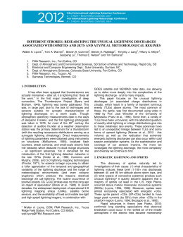
Figure 1.2 depicts the life cycle GHG emissions from a set of vehicles (hybrid EV, plug-in
hybrid EV with 30, 60 and 90 km of range, classical combustion vehicle) as a function of the
life cycle GHG intensity of the power system [20]. The small slope in the combustion vehicle
and hybrid EV is related to the electricity used for vehicle manufacturing. For the plug-in
EV, this picture indicates that with a low carbon generation portfolio the GHG emissions of
3
1.1. General Context and Motivation
Figure 1.2: Life cycle GHG emissions from vehicles shown as a function of the life cycle GHG intensity of
electricity generation [20].
plug-in hybrid EV are lower compared to a hybrid EV, but for coal-based power systems the
emissions are higher than the ones for hybrid EV.
Therefore, the development and investment in EV should be complemented with decarbonization policies for the electric power system, such as investment in RES-E, more flexible resources in the supply and demand-side, and participation of distributed generation in ancillary
services.
The second aspect, and which is related to this PhD thesis, is that, even in countries with a
high penetration of RES-E, if the EV are charged during peak hours, peak power units with
intensive GHG emissions are likely to be dispatched, which undermines the benefits from
EV. This is likely to happen if the EV charging is uncontrollable, e.g. the EV starts charging
when the drivers plug-in at home after returning from work. This uncontrollable charging can
increase the GHG emissions [21] and create technical problems in the distribution network
[22] (e.g., branches congestion and voltage limits violation).
Therefore, in order to take full advantage of the EV benefits to the system and avoid technical
problems, it is essential to directly control and coordinate the charging process of each EV.
For instance, a coordinated strategy of EV charging can help to decrease the power losses and
branch congestions, as well as to improve voltage profiles [23]. Moreover, direct control also
enables the provision of ancillary services (e.g., reserves) from the EV [24].
The backbone that enables EV charging control is a smart grid infrastructure [25], which
provides additional capabilities for the observability and controllability of the distribution
network level, and is strongly supported by the Information and Communications Technology
(ICT) and the Advanced Metering Infrastructure (AMI). This enables new features, such as
4
1.1. General Context and Motivation
a two-way communication infrastructure, which creates conditions for demand response and
dispatch.
The massive deployment of the EV and necessary interaction with the power system operators
of transmission and distribution networks can be supported by an agent responsible for aggregating EV and managing their charging process within the smart grid paradigm [26]. This
agent is called aggregator and it is an enabler of the EV integration in the electricity market
and power system operation. From the system operators’ viewpoint, the EV aggregator is part
of a hierarchical control architecture and coordinates the EV charging in response to the system operators’ signals, which decreases their communication requirements [23]. From the EV
owners’ viewpoint, the aggregator uses their available flexibility to purchase electrical energy
at low price and sells ancillary services in the electricity markets, which ultimately lead to a
retailing tariff reduction.
The combination of a smart grid infrastructure, direct control of EV charging and aggregators
entails the following benefits that cover economic, environmental and social aspects:
• with the electric power sector unbundling, the economic signals and incentives for
future investments in generation capacity generally come from the electricity market
prices. With the increasing penetration of RES-E, the market prices are showing a declining tendency (in some cases are even negative [27]), which decreases the incentives
to build additional and more flexible generation capacity to handle RES-E variability and
uncertainty, and can put offline secondary and tertiary reserve resources when needed.
Nevertheless, countries with a significant penetration of EV can use this existing flexible demand-side resource and postpone the need to create financial instruments (e.g.,
capacity markets or tariffs) that encourage investments in flexible generation capacity.
This also postpones investments in flexible conventional power plants;
• it creates conditions for integrating high penetration of RES-E, since it contributes to
avoiding curtailment of RES-E during valley hours, and its flexibility and fast response
capability support the system in handling variability and uncertainty of RES-E (e.g.,
through the provision of reserve services);
• shifting EV load to valley hours allows conventional power plants to run at a higher load
factor, improving their efficiency and reducing GHG emissions;
• compared to a situation with uncontrolled EV charging, controllable charging reduces
the peak load and decreases the need to invest in additional conventional peak power
plants;
• it introduces new competition in the ancillary services market, reduces the amount of
5
1.1. General Context and Motivation
reserve power used from conventional power plants, and contributes to a more active
participation from the demand-side in these services;
• it encourages competition and innovation in the electricity retail market. For instance,
electricity retailers might expand their products, such as adopting a retailing tariff closer
to the wholesale market price, and create financial incentives for inducing a more flexible and price-responsive behavior of the loads. In this case, the consumer benefits from
a decrease in the final cost of electricity and is encouraged to make behavioral changes.
These benefits and various features of sustainable development can only be activated with
an adequate coordination between EV aggregators and system operators within the smart
grid infrastructure. This coordination requires interdisciplinary computational models (from
operations research, statistics, data mining, etc.) that support the EV aggregator activity and
its integration in the power system. This interdisciplinary framework is called computational
sustainability [28], and is defined as “new computational models, methods, and tools to help
balance environmental, economic and societal needs for sustainable future” [29].
Related to this context and considering the potential benefits from EV aggregators for the
power system, this PhD thesis aims to contribute with a set of computational tools that support the participation of plug-in hybrid and battery EV in the electricity market, enabling the
provision of secondary and balancing reserve services from this agent and ultimately supporting an increasing penetration of RES-E. The goal is to have demand-side treated equally with
the supply-side and provide similar services (e.g., secondary and balancing reserve) without
compromising power system reliability.
This research work was driven by the following research question:
Which decision-aid methods are required by an EV aggregator to participate in
the electricity market and perform economical and technical management of its portfolio?
Even with the possibility of collecting a large amount of information, there are information
gaps and also inherent uncertainties such as the drivers’ behavior and electricity market prices.
Therefore, this activity requires a chain of computational models divided into three phases:
forecast, day-ahead optimization and operational management. The forecasting phase provides the inputs of the day-ahead optimization that determines the “optimal” bids for the
electricity market. An operational management algorithm is used, during the operating day,
to coordinate the EV charging and comply with the market commitments; the actual charging
decisions of the EV fleet result from this operational phase.
These algorithms take into account the current power system design, which includes a liberal6
1.2. Objectives of the Thesis
ized electricity market environment, and minimize the aggregator’s wholesale cost. Therefore,
EV charging follows economic signals given by the electricity market, but from a demand-side
perspective that results in some benefits to the power system. For instance, moving EV charging from high prices (i.e., peak hours) to low prices (i.e., valley hours) periods increases
the efficiency of conventional generators that operate with low load factor during valley
hours. During valley hours, the occurrence of situations with RES-E surplus (in particular
wind power) might be frequent and the EV charging contributes to the decrease wind power
curtailment.
Furthermore, EV aggregators with suitable management procedures, such as the operational
management algorithms proposed in this PhD thesis, help decrease forecast errors associated
to EV charging, since one objective consists in minimizing imbalance costs. An EV aggregator that operates its EV fleet charging in response to reserve prices (i.e., cheap charging as
downward reserve and income from selling upward reserve) uses its flexibility to handle imbalances from other market agents (e.g., wind farms), and since it can offer bids at a very low
marginal price, it also helps decrease the system operational costs (which are included in the
consumers’ final tariff).
Finally, by discussing the role of an EV aggregator, the framework to support its participation
in the electricity market and necessary computational tools for enabling its operation, we are
moving the discussion from the supply to the demand-side. The discussion is about finding
solutions in the demand-side that support the increasing share of electrical energy from RESE, and developing appropriate computational tools that enable the integration of RES-E from
the electrical power system in the transport sector.
1.2 Objectives of the Thesis
The work presented in this thesis involves the development of new computational tools for
supporting the EV aggregator participation in electricity markets. The main objectives are:
• to define a model for the EV aggregator that includes a framework with the necessary
computational algorithms for each market session, available information and communication flows and commercial relations with stakeholders;
• to formulate optimization problems, which use forecasts as input, to support the EV
aggregator in defining the “optimal” and robust bids for the energy, secondary and
balancing reserve market sessions and without considering the vehicle-to-grid (V2G)
concept;
7
1.3. Structure of the Thesis
• to formulate operational management algorithms that coordinate the EV individual
charging in order to minimize imbalance costs due to deviations between accepted bids
and actual charging, and avoid reserve shortage situations;
• to study the sources and effects of uncertainties in the optimization results. The optimization results should provide information about the impact of forecast errors in the
total wholesale cost and reserve shortage magnitude;
• to refine our current understanding of the electricity market rules to accommodate this
new market agent. Although this is not a main objective, the optimization models results
should lead to a set of suggestions for adjusting the current electricity market protocols
in order to better accommodate EV.
1.3 Structure of the Thesis
The work developed within the scope of this PhD thesis is organized into seven chapters
(including the present one).
The current chapter 1 presents the general context and motivation to this PhD thesis, defines
the problem under research and its main objectives.
Chapter 2 is a literature review about the integration of EV in the power system and electricity
market, covering technical and economic perspectives, as well as optimization algorithms for
supporting the EV aggregator participation in the electricity market. Relevant background for
this topic, such as power system reserves and electricity markets, is also presented.
The aggregator model (e.g., architecture, economic, physical and information flows), and
a framework for the electricity market sessions with corresponding optimization/forecasting
algorithms are described in chapter 3.
The following three chapters propose optimization problems covering different electricity
market sessions, illustrated with the same test case composed of synthetic EV time series
and market data from the Iberian electricity market. Each chapter has its own results section.
The participation of the EV aggregator solely in the day-ahead electrical energy market is
addressed in chapter 4. Two alternative optimization approaches, global (uses forecasts for
aggregated EV variables) and divided (uses forecasts for EV variables of each vehicle), are
described and compared. An operational management algorithm that coordinates the EV
individual charging in order to minimize imbalance costs is also described and evaluated. The
8
1.4. List of Publications
impact of forecast errors in the total wholesale cost is estimated.
Chapter 5 formulates a day-ahead optimization problem for energy and secondary reserve
bids and an operational management algorithm that coordinates EV charging in order to
minimize differences between contracted and realized values of energy and secondary reserve.
Chapter 6 covers the participation of an EV aggregator in a reserve intended to solve energy
imbalances between scheduled and realized values for the system, generally resulting from
renewable generation forecast errors. A day-ahead optimization problem is formulated for the
electrical energy and balancing reserve bids, and two operational management algorithms,
one for day-ahead bids and another for hour-ahead bids, are proposed for this balancing
reserve.
Chapters 5-6 also estimate the impact of forecast errors in the total cost and reserve shortage
magnitude.
The main document ends with chapter 7, where the main contributions, findings and topics
for future work are described.
Three appendices complement the main document.
Appendix A presents statistical analyses of the synthetic EV time series and market data used
in the test case. Appendix B presents the forecast error analyses of the EV and market prices
time series. Appendix C describes two heuristic operational management algorithms from the
state-of-the-art and that were enhanced by Lima [30]. These two algorithms are compared
with the operational algorithm proposed in chapter 4.
1.4 List of Publications
International Journals
• (Chapter 2) R.J. Bessa and Manuel A. Matos, “Economic and technical management of
an electric vehicles aggregation agent: a literature survey,” European Transactions on
Electrical Power, vol. 22, no. 3, pp. 334-350, Apr. 2012.
• (Chapter 4) R.J. Bessa and M.A. Matos “Global against divided optimization for the
participation of an EV aggregator in the day-ahead electricity market. Part I: theory,”
Electric Power Systems Research, vol. 95, pp. 309-318, Feb. 2013.
• (Chapter 4) R.J. Bessa and M.A. Matos “Global against divided optimization for the
9
1.4. List of Publications
participation of an EV aggregator in the day-ahead electricity market. Part II: numerical
analysis,” Electric Power Systems Research, vol. 95, pp. 319-329, Feb. 2013.
• (Chapter 5) R.J. Bessa, Manuel A. Matos, F.J. Soares, and J.A. Peças Lopes, “Optimized
bidding of a EV aggregation agent in the electricity market,” IEEE Transactions on Smart
Grid, vol. 3, no. 1, pp.443-452, Mar. 2012.
• (Chapter 5) R.J. Bessa and M.A. Matos, “Optimization algorithms for an EV aggregator
selling secondary reserve in the electricity market,” paper under review in Electric Power
Systems Research, 2013.
• (Chapter 6) R.J. Bessa and M.A. Matos, “Optimization models for EV aggregator participation in a manual reserve market,” IEEE Transactions on Power Systems, in press, 2013.
(doi: 10.1109/TPWRS.2012.2233222)
International Conferences
• (Chapter 3) R.J. Bessa and M.A. Matos, “The role of an aggregator agent for EV in
the electricity market,” in Proceedings of MedPower 2010, Agia Napa, Cyprus, 7-10 Nov.
2010.
• (Chapter 4) R.J. Bessa, N. Lima, and M.A. Matos, “Operational management algorithms
for an EV aggregator,” in Proceedings of MedPower 2012, Cagliari, Italy, 1-3 Oct. 2012.
• (Chapter 5) R.J. Bessa, F.J. Soares, J.A. Peças Lopes,and M.A. Matos, “Models for the
EV aggregation agent business,” in Proceedings of IEEE PowerTech 2011, Trondheim,
Norway, 19-23 June 2011.
• (Chapters 4-6) R.J. Bessa and M.A. Matos, “Forecasting issues for managing a portfolio
of electric vehicles under a smart grid paradigm,” in Proceedings of the Third IEEE PES
Innovative Smart Grid Technologies (ISGT 2012), Berlin, Germany, 14-17 Oct. 2012.
National Conferences
• (Chapter 4) R.J. Bessa and M.A. Matos, “Two alternative approaches for modelling a
portfolio of electric vehicles,” 1st PhD. Students Conference in Electrical and Computer
Engineering, Faculty of Engineering, University of Porto, Portugal, 28-29 Jun. 2012.
• (Chapter 5) R.J. Bessa and M.A. Matos, “Alguns problemas de optimização para um
agente agregador de veículos eléctricos. Optimization problems for an EV aggregation
agent,” presentation in the 15◦ Congresso Nacional da Associação Portuguesa de Investigação Operacional, Coimbra, Portugal, 18-20 Apr. 2011.
10
Chapter
2
Background and State of the Art
Abstract
This chapter presents a literature review about the integration of EV in the power system and electricity market, from technical and economic perspectives and with particular emphasis on the role
of an EV aggregator. Moreover, optimization algorithms for supporting the EV aggregator participation in the electrical energy and ancillary services market are reviewed. Relevant background for
this topic, such as power systems reserves and electricity markets, is also presented.
2.1 Introduction
Primarily, the EV1 is an additional electric load in the power system, characterized by a significant temporal uncertainty of its consumption value. However, in a Smart Grid environment,
it is possible to control the EV charging or even inject power from the EV batteries into the
electrical network [called Vehicle-to-Grid (V2G)].
The present state of the art in the topic of EV is mainly devoted to study the integration of
EV in the electrical network and power system operations. Different authors are studying the
EV integration, exploring scenarios where EV are additional loads, but also scenarios where
EV are controllable loads that could include or not the V2G capability. Generally, the outcome
of this research is that new management procedures, with a strong link to the Smart Grid
paradigm, allow a massive integration of EV and mitigate impacts on voltage profiles, power
losses and branch congestions. It is not an objective of this chapter to present a detailed
1
In this thesis the acronym EV means plug-in battery or plug-in hybrid vehicles if nothing more is added.
11
2.2. Background
review on this topic, thus only the relevant results are briefly presented in section 2.3.
The literature review will be mainly focused in two research directions. The first one is related to the economic and technical value of EV in the electricity market (section 2.4). The
aggregation of EV was found to be technically attractive and economically valuable and, in
general, to favor the deployment of EV, if a good business model is adopted. Thus, business
models for an EV aggregator are also reviewed.
The second one, in section 2.6, is related to optimization algorithms developed to support the
participation of an EV aggregator in the electricity market.
This chapter also presents the relevant background for this topic (section 2.2), which contains
a description of the power system reserves, electricity market and demand-side integration.
2.2 Background
2.2.1 Power System Reserves
Reserve Definitions
In each time instant, the Transmission System Operator (TSO)2 is responsible for managing the load-generation mismatch in the power system. A positive imbalance (generation
greater than load) will increase the system frequency above its nominal value (50 or 60 Hz),
and a negative imbalance (load greater than generation) will decrease the system frequency.
This leads to the need of an upward and downward reserve capacity composed of loads and
generation units able to respond to frequency disturbances. The upward reserve consists of
generation units (or loads) online or offline able to, in a short period, increase their generation levels (or decrease their consumption levels). The downward reserve consists of online
generation units able to decrease their generation levels or loads able to start consuming (or
increase consumption) in a short period. The nomenclature and technical characteristics of
reserve categories are different across several countries, even inside the same interconnected
system [32].
The classical reserve categories, depicted in Figure 2.1, are defined by the European Network
2
In the USA a different nomenclature is used: Independent System Operator (ISO) and Regional Transmission
Organization (RTO). Both have the same functions of the TSO in Europe, but the main difference is that the ISO
usually operates only within a single USA state, while the RTO operates over large interstate areas. A detailed
comparison between TSO, ISO and RTO can be found in [31].
12
2.2. Background
of Transmission System Operators for Electricity (ENTSO-E) Operational Handbook as:
• primary control reserve: “joint action of all interconnected TSO, primary control stabilizes the system frequency at a stationary value after a disturbance or incident in the
time-frame of seconds, but without restoring the system frequency and the power exchanges to their reference values. The time for starting the action is a few seconds after
the incident, the deployment time for 50% or less of the total primary control reserve is
at most 15 seconds and from 50% to 100% the maximum deployment time rises linearly
to 30 seconds. Primary control power must be delivered until the power deviation is
completely offset by the secondary/tertiary control reserve of the control area in which
the power deviation has occurred.” [33];
• secondary control reserve: “is used to keep or restore the system frequency to its setpoint value of 50 Hz and the power interchanges with adjacent control areas to their
programmed scheduled values, thus ensuring that the full reserve of primary control
power activated will be made available again.” [34]. “Secondary control makes use of a
centralized and continuous Automatic Generation Control (AGC), modifying the active
power set points / adjustments of generation sets/controllable load in the time-frame
of 30 seconds (at the latest) up to typically 15 minutes (at the latest) after an incident”
[33];
• tertiary control reserve: “is usually activated manually by the TSO in case of observed or
expected sustained activation of secondary control. It is primarily used to free up the
secondary reserve in a balanced system situation, but it is also activated as a supplement
to secondary reserve after larger incidents. Schedule activated tertiary control reserve
is activated with relation to the predefined timeframe of exchange schedules, e.g. 15
minutes” [33].
The Nordic countries (forming the Nordel network) are not connected to the Union for the Coordination of Transmission of Electricity (UCTE) interconnected network (with the exception
of West Denmark) and their reserve nomenclature is different [35]. Nevertheless, in technical
terms the use of the reserves is rather similar.
The primary reserve is divided into normal and disturbances automatic frequency controlled
reserve, and secondary reserve is called load frequency control. Other types of reserves are
required for full restoration of imbalances. These reserves are mostly manually activated and
used to restore the balance after deviations (e.g., forecast errors) during the operating hour
and to relieve the frequency controlled reserves. The activation time of these reserves is less
than 15 minutes.
13
2.2. Background
System
Frequency
Primary
Control
Secondary
Control
Tertiary
Control
Time
Control
Figure 2.1: Frequency control scheme and actions of the ENTSO-E operational handbook [33].
The nomenclature of ENTSO-E is presently being revised in the “Draft Network Code on LoadFrequency Control and Reserves” [36] that is under public consultation. Primary reserve
will be named frequency containment reserve, secondary reserve named frequency restoration
reserve and tertiary reserve named replacement reserve. Nevertheless, the definitions are rather
the same.
In the USA, the reserve nomenclature and categories are also different across the North American Electric Reliability Corporation (NERC) jurisdiction. Nevertheless, the three control types
of the ENTSO-E definitions can also be found [37]. The primary frequency control is frequently called primary frequency response and the secondary control is often referred to as
regulation reserve [38]. The tertiary control is often referred to as ramping or load-following
reserve [37].
The difference between the USA and Europe is that contingency reserves are explicitly defined
in North America while they are not in Europe [39]. Contingency reserves are mainly considered for handling forced outages of conventional generation. Kirby [40] presents a reserve
description, depicted in Figure 2.2, that is reasonably consistent across North America. The
primary, regulation and load following reserve are included in the group of reserves for normal
conditions (i.e., compensates for the variability and uncertainty of load), while the reserves for
contingency conditions are: spinning, non-spinning and replacement (or supplemental) reserve.
Spinning reserve is defined as “online generation, synchronized to the grid, that can increase
output immediately in response to a major generator or transmission outage and can reach
full output within 10 min”. Non-spinning reserve is the “same as spinning reserve, but need
not respond immediately; resources can be offline but still must be capable of reaching full
output within the required 10 min”. The replacement reserve “is used to restore spinning and
14
2.2. Background
Replacement or Supplemental Reserve
Contingency Operations
Non-Spinning Reserve
Spinning Reserve
Normal Operations
Load Following or Energy Imbalance
Regulation
Voltage Control
0.1
1
10
100
TIME (MINUTES)
Figure 2.2: Response time and duration of different reserve categories in the USA [40].
non-spinning reserves to their pre-contingency status; it must have a 30-60 minutes response
time.”.
Redefinition of the Reserve Nomenclature
For countries with high penetration of RES-E (mainly wind and solar), Holttinen et al. [41]
revised the reserve nomenclature: non-event (normal operation) for variability and forecast
errors inside the scheduling period; fast-event (contingency operation) for unplanned outage
of a generator or cross-border transmission line; slow-event for net-load ramps and forecast
errors that can occur in longer time-scales (from ten minutes to hours). The authors argue
that RES-E based generation does not change faster enough to be a contingency event and the
impact in secondary reserve is lower (c.f., [42][43]) than the impact on tertiary reserve (both
reserves are included in the non-event category). High penetrations of RES-E based generation
will introduce slow-events characterized by high generation ramps and forecast errors.
In the time-scale of tertiary reserve, several countries have already created a reserve category
for slow-events. For instance, the Spanish power system has a deviations reserve that is only activated for load-generation deviations above 300 MWh [44]. In Denmark, the manual reserve
is used to handle forecast errors. The Hydro-Quebec power system includes an energy balancing reserve for handling forecast errors [43]. In the USA, it is under discussion the creation of
a ramping reserve [45].
Conversely, in Portugal, the tertiary reserve3 is used to compensate forecast errors [47]. Elec3
In fact, in Portugal tertiary reserve is called reserva de regulação [46], but this term is not used because its
English translation is regulation reserve, which could create confusion with a reserve category in U.S.A. that
has the same name but a different function.
15
2.2. Background
tric Reliability Council of Texas (ERCOT) uses the non-spinning reserve for handling wind
power forecast errors [48].
In this thesis, the reserve is divided into the following categories according to its main functions:
• frequency reserves: classical reserve categories (i.e., primary, secondary and tertiary frequency control) that are procured by the TSO/ISO for handling frequency excursion
problems;
• balancing reserve: active power manually requested by the TSO/ISO to handle forecast
errors and ramp up/down events related to RES-E generation. This reserve is slower
than frequency reserve and the TSO will procure this type of reserve for handling positive and negative imbalances of the market schedule.
2.2.2 Electricity Markets
Figure 2.3 depicts the general structure of an electricity market, which will be reviewed in
this section.
Futures Market (E)
Bilateral Contracts (E+AS)
Tenders (AS)
Day-ahead
Market (E+AS)
Bilateral
Contracts (E)
Intraday,
Hour-ahead
and Real-!me
Markets
(E+AS)
…
…
Days, weeks, months, years
before
Payment for
Imbalances
Day (D)
Opera!ng Day
(D+1)
Time
Spot Market
Figure 2.3: Structure of the electricity market (E: Electrical energy; AS: Ancillary services).
The electricity market can be divided into two different types [49]: the spot market, where
the electrical energy and ancillary services4 are traded for immediate physical delivery, and
the futures market, where the delivery is at a later date and normally does not involve physical
delivery. The futures market is normally used for risk hedging [50]. In this section, emphasis
is given to the spot market.
4
Ancillary services are functions separated from the electrical energy market, which are used to support reliability and power quality of the power system. One example is the power system reserves.
16
2.2. Background
Coexisting with the electricity market, there are also bilateral contracts that the market agents
are free to trade. These contracts are normally used to guarantee a certain amount of electrical
energy for the demand-side, or to guarantee a certain profit for the supply-side, or used as a
risk hedging mechanism.
Typical European Spot Markets
A typical European electricity market can be operated by the TSO or by a pool operator. The
pool operator establishes relations with generators, distribution companies, retailers, eligible consumers and the TSO. The pool operator or TSO runs a centralized market-clearing
algorithm.
The spot market can be divided into two main categories: electrical energy and ancillary
services. The electrical energy market is divided in day-ahead and intraday (or hour-ahead)
sessions.
The day-ahead electrical energy market is a double-side auction where the supply-side (i.e.,
agents with generation units) submits bids (i.e., minimum price they want to receive and
quantity) that are ordered by ascending price and cumulative quantity (named supply curve)
and the demand-side (i.e., agents with loads) submits bids (maximum price they want to pay
and quantity) that are ordered by descending price (named demand curve). The point of
intersection of these two curves is the market-clearing price, which is a uniform price since
all the market agents pay/sell the electrical energy at this price value. An alternative auction,
which is uncommon to find in electrical energy markets, is called pay-as-bid price auction. In
the pay-as-bid system, the supply-side sells the cleared quantity at the offered bid’s price (the
same is valid for the demand-side).
The market gate closure5 is normally before noon. The market agents may present buy and
sell hourly bids that cover all 24 hours (or 48 half-hours in some markets) of the next day
(or operating day). Different types of bids are possible: a price independent bid for all hours
regardless of the price level, with only a price cap and floor; a price dependent hourly bid for
all hours where a stepwise curve is submitted (i.e., different quantities for different prices);
complex bids that can include inter-temporal constraints of the generation units (e.g., ramp
constraints) or minimum revenue requirement (e.g., start up and down costs).
After the market-clearing, the TSO performs constraints management (i.e., solves network
congestion and voltage limits violation). The procedure to solve technical constraints modifies
5
Time instant when participants cannot modify their bids any-more.
17
2.2. Background
the day-ahead schedule and determines which selling and buying offers should be added or
removed from the initial daily program of operation. In electricity markets with more than one
control area and in case of congestions between interconnected areas, the market is separated
into lower/higher price areas.
There are a few countries without a day-ahead energy market. One example is the British
Electricity Trading and Transmission Arrangements (BETTA), which moved from a pool trading to a free bilateral trading operating on a rolling half-hourly basis and one hour-ahead of
actual supply (gate-closure is one hour before) [51].
Intraday markets are conceptually analogous to day-ahead energy markets and the main difference is the gate closure. Essentially, it follows the day-ahead session, and works as an
adjustment market close to the operating hour. In these cases, with additional and/or more
accurate information, the market agent can correct the accepted bids from the day-ahead
market or from previous intraday sessions.
Two structures of intraday markets can be found:
• continuous trading that takes place after the day-ahead market and with a gate closure
of one hour before physical delivery. One example is the Elbas session from NordPool
[52];
• fixed number of sessions at pre-defined periods and for the remaining hours of the
operating period. One example is the Iberian electricity market, which has six intraday
market sessions [53].
The majority of these intraday markets are non-mandatory and present a low liquidity [52][54].
The ancillary services are divided in reserve services and other services (e.g., voltage control,
black start). The mechanisms for procuring reserve differ from country to country and from
category to category. In general, the TSO is responsible for procuring these services and different mechanisms can be used: mandatory and non-remunerated; monthly or yearly tenders;
bilateral contracts; electricity market (i.e., on a daily basis) [55].
For example, in the Nordic countries, the automatic frequency controlled reserves are acquired by TSO using different types of contracts with generators [35]. In Germany, there is
a competitive tendering for primary and secondary control reserve that takes place every six
months and is organized by the TSO for its control area [56]. The primary reserve is traded
only with a capacity price bid, while secondary reserve is traded with a price for available
and dispatched capacity. In other countries, such as Portugal and Spain, primary reserve is
mandatory and non-remunerated [55]. In France, the secondary reserve is procured with bi18
2.2. Background
lateral contracts between TSO and generators with a pay-as-bid-price for both net energy and
capacity [55].
The secondary reserve can also be procured with day-ahead auctions in the electricity market.
For example, in Portugal and Spain, there is a market pool for secondary reserve [53]. The
agents present capacity bids (quantity in MW and price in C/MW), and the amount of reserve
contracted to each unit is settled at the marginal price of the secondary reserve market. The
dispatched reserve price (price in C/MWh) is defined by the price that results from the tertiary
reserve market. In Portugal, the TSO defines a ratio between upward and downward reserve
capacity [57][58]. Another country with a day-ahead market for secondary reserve is Italy
[59], but with a pay-as-bid-price system and mandatory participation.
Tertiary reserve is contracted for the next day or during the operating day [54]. For example,
in NordPool the manual reserve is purchased in the regulating power market, with a gate
closure of 45 minutes before the operating hour. The bids presented by the market agents
(called production and load balancing responsible) are placed in priority order according to
the price and the TSO uses this list as far as possible to handle imbalances due to forecast
errors [35].
The tertiary reserve bids in Portugal and Spain are presented for the next day (at 23h00) to
the TSO and the market agents can continuously update and modify these bids until one hour
(in Portugal) and 45 minutes (in Spain) before the operating hour. The TSO, has for each
hour, a list of bids, which are used when it is necessary (i.e., can be called 15 minutes before
and during the operating hour) to handle forecast errors and/or replace secondary reserve
[54]. There is only a single price for dispatched reserve power and maximum duration is
usually one hour. In Spain, there is also a deviations reserve market that takes place between
intraday sessions and the agents can present bids one hour before the time horizon of the
corresponding balancing market session [58].
In Germany, upward and downward tertiary reserve (or minute reserve) is procured on a
daily basis after the energy market for six four-hour time slots of the next day [60]. Tertiary
reserve is traded with two prices, one for available capacity and another for dispatched power.
In Italy, there are five balancing market sessions with pre-defined opening and gate closure
times where reserve services are procured for solving imbalances and congestions [59]. The
participation is mandatory and with a pay-as-bid price.
Other type of ancillary services, such as voltage control, are normally mandatory and nonremunerated, or remunerated with bilateral contracts [55].
Imbalance prices (or financial penalizations), for both positive and negative deviations from
19
2.2. Background
schedule, result from the use of reserves for solving imbalances, and these prices reflect the
costs incurred by the TSO for delivering electrical energy in real-time [61].
For example, in Portugal, the imbalance prices are tariffs related to the costs of contracting
and using reserves (secondary and tertiary), while in the NordPool, the imbalance prices are
the clearing price of the regulating power market (i.e., manual reserve). Two possibilities
exist for imbalance prices: single (or symmetrical) price and double (or asymmetrical) price
for negative and positive deviations. Some countries like Germany and the Netherlands have
a single imbalance price, while others, like Portugal and Denmark, have a double price [54].
In most cases, deviations opposite to the total system deviation are not penalized (i.e., they
are valued at the electrical energy price from the last day-ahead or intraday market session).
USA Spot Markets
The USA markets have two fundamental differences to the European markets. First, the price
is calculated for every node [called Locational Marginal Price (LMP)] of the transmission
network [62]. The LMP reflects the cost of generation in specific nodes. For instance, when
there is transmission congestion, the generation with lower cost cannot supply the loads in
certain locations and, in this case more expensive generation is scheduled to meet these loads
and the LMP is higher in those nodes.
The second difference is the market-clearing mechanism. Ellison et al. [63] identified three
different clearing mechanisms:
• integrated joint-optimization: prices and schedule of energy and reserves are determined
simultaneously by an optimization problem with a single objective function and a set
of constraints. The ISO with this mechanism are Midwest ISO (MISO), New York ISO
(NYISO), California Independent System Operator (CAISO) and ERCOT.
• coupled joint-optimization: separated optimization for energy and reserves, but both
optimization problems have coupled constraints (e.g., the energy optimization contains
inequality constraints related to reserve requirements). The Pennsylvania-New JerseyMaryland Interconnection (PJM) uses this mechanism.
• decoupled optimization: separated optimization of energy and reserve without coupled
constraints (i.e., similar to the European markets). The ISO New England (ISO) uses
this mechanism.
There is also a real-time market in the USA which performs functions similar to the intraday markets in Europe. The gate closure of this market varies widely across ISO, ranging
20
2.2. Background
between 30 and 75 minutes before the operating hour. Financial penalties are considered for
imbalanced energy from the day-ahead or real-time schedule [64].
In the real-time market, the agents can present reserve bids, but in cases, such as the NYISO
[65] and CAISO [62], the majority of the reserve is procured in the day-ahead market.
2.2.3 Demand-side Active Participation
One of the goals of the Smart Grid paradigm is to enable the transmission of direct control or
price signals to reduce consumptions during peak hours or emergency situations [66]. This is
achieved by integrating Information and Communications Technology (ICT) [e.g., Advanced
Metering Infrastructure (AMI)] and advanced control technologies into the power system.
With the availability of bidirectional communication, distributed sensors (e.g., phasor measurement units), advanced data mining and optimization techniques, a proactive participation
of the demand-side in the electricity market is feasible and expected.
Europe
Torriti et al. [67] presented an overview of the Demand Response (DR) programs in Europe.
According to the authors, this mainly consists of long-term contracts or programs to promote
the DR participation of large industrial consumers, through interruptible tariffs and time-ofuse tariffs. For example, in Spain, Portugal and Italy the DR mainly consists of interruptible
contracts for large consumers which receive curtailment signals from the TSO some time in
advance. For small consumers the only incentive is a time-of-use tariff.
However, this is changing in Europe, in particular with the deployment of the Smart Grid
paradigm [25]. For example, in [68] it is mentioned that the TSO of Norway (Statnett) is
developing action plans for acquiring 260 MW of DR through both tendering and market
bidding, mainly focused on medium-size end-users and independent aggregators.
The TSO of Denmark (presently Energinet.dk), in order to promote the participation of small
loads in the regulation power market, published a proposal in 2010 for the following years
which outlines two methods [69]:
• participation in the regulation power market under the current rules and to overcome
the minimum bid size constraint (10 MW) it will be allowed to aggregate assets on the
demand-side;
21
2.2. Background
• self-regulation: the price of the regulation power market6 will be published during the
operating hour (in opposition to one hour after the operating hour) and in this model
the small loads units will have the chance to self-regulate in accordance to this price.
This service can be divided into two types: (a) the balance responsible has direct control
over some loads (e.g., heat-pumps, electric boilers); (b) the balance responsible defines
the electricity tariff according to the regulation price (and its business model) and the
end-user reacts to the tariff value.
Finally, in Germany, the Federal Network Agency defined new conditions for the primary
and secondary reserve tenders [70]. The goal was to enable access from small generators,
loads and storage. For primary reserve, the main changes were: reducing the tender horizon
from one month in advance to one week; reducing the minimum bid from 5 MW to 1 MW;
the possibility to aggregate resources. For secondary reserve, the changes were similar, but
minimum bid was reduced from 10 MW to 5 MW.
USA
In the USA, there is an increasing share of DR programs and integration in the electricity
market. Kirby et al. [71] present an overview of the current situation. The experience
of having loads supplying ancillary services is limited to the markets of ERCOT, MISO, PJM,
NYISO and some pilot projects in ISO-NE, Bonneville Power Administration (BPA) and CAISO.
In PJM, around 250 MW of spinning reserve is from demand-resources and half of the spinning
reserve in ERCOT comes from loads. Similarly to Europe, almost all loads are industrial or
large consumers. MISO uses loads for regulation reserve; PJM and BPA also have pilot projects
with loads supplying primary reserve. Interruptible loads (based on low frequency threshold
or ISO signal) participate in contingency reserves in ERCOT, MISO, PJM and NYISO.
In the restructured market of ERCOT, the role of demand was enhanced and a set of DR types
were created [72]. One of these types was LaaR (load acting as a resource). The idea of LaaR
is to have loads directly competing with generators to provide several ancillary services (e.g.,
non-spinning reserve) procured in the day-ahead market. In 2008, the level of participation in
LaaR was around 1300 MW, but this available capacity consists of large and medium industrial
and commercial facilities.
Another example is the PJM market, which allows the participation of Curtailment Service
Providers (CSP) that aggregate demand resources to reduce load [73][74]. The CSP can
participate in PJM Economic Load Response market that enables demand resources to reduce
6
Latest activated regulation power unit.
22
2.2. Background
consumption in response to energy, spinning reserve and/or day-ahead supplemental reserve
prices, or follow a PJM regulation signal to reduce or increase load. The participation of loads
in the spinning reserve market increased during the last years and, presently, loads provide
17% of this reserve (mainly industrial consumers). There is no participation of loads in the
regulation reserve market.
The participation of residential loads in the DR programs is minimal and it only exists at
pilot projects level [71]. One example is the Demand Response Reserves Pilot Project from
ISO-NE for single or aggregated load resources providing a service similar to the forward
reserve market in ISO-NE [75]. The program was primarily designed to supermarkets, big-box
retailers and aggregators of residential air-conditioning with direct control, until a maximum
load reduction of 5 MW.
Reserve Shortage in DR Programs
The authors of [40] and [71] mentioned the fact that forecasting the load participation in
ancillary services might be a difficult task. Several factors (e.g., nature of the load, control
algorithms, aggregation size) could make difficult to deliver the contracted energy. Therefore,
it is important to develop mechanisms that mitigate this problem.
Some TSO/ISO already have penalty terms for situations with reserve capacity shortage. For
example, ISO-NE has two penalty terms for the forward reserve market7 [75]: failure-toreserve penalty that is imposed when the available reserve capacity in that hour is less than
the capacity contracted in the market; failure-to-activate is imposed when a resource failed to
activate or reduce load when requested to do so by the ISO within 10 or 30 minutes. Between
2008 and 2010, the failure-to-activate term was very low, compared to the failure-to-reserve
penalty, which ranged between 3% and 4% of the forward reserve payment [76].
PJM and CAISO have recently introduced a pay-for-performance compensation for resources
providing regulation reserve8 . PJM uses three components [77]: accuracy score is the correlation between control signal and regulating unit’s response; delay score is the time delay
between control signal and point of highest correlation from the accuracy score; precision score
is a function of the difference in the energy provided versus the energy requested by the regulation signal.
7
8
The forward reserve market has seasonal auctions (summer and winter) and comprises obligations of 10-min
non-spinning reserve and 30-min operating reserve.
http://info.a123systems.com/blog/bid/133226/New-California-ISO-Frequency-Regulation-Rules-Favorableto-Grid-Energy-Storage (accessed in March 2013)
23
2.3. Integration of EV into the Power System
These three components make a performance score that is included in the clearing process.
Poor performing resources will appear more costly and thus less desirable. For instance, a 20
MW resource with a 0.25 performance score would appear as costly as an 80 MW resource
with a 1.00 performance score. The NYISO also has a factor (between 0 and 1) related to the
regulation service performance (i.e., capability of following the AGC signal) [78].
In Portugal, there is also a penalization term for situations with secondary reserve capacity
shortage [57].
2.3 Integration of EV into the Power System
2.3.1 Early Studies
The first studies about economic and technical problems resulting from the massive integration of EV in the power system were mainly characterized by the following aspects:
• EV were merely additional loads for charging batteries [79][80];
• two alternative charging strategies were used for assessing the EV impact: (a) charging
begins when the drivers park the EV; (b) a time-of-the-day pricing induces the driver
to charge the EV in periods when the electricity price is lower (e.g., low-load periods)
[79][81];
• the distribution network was not included in the studies [79][80][82].
Two important conclusions were relevant for future studies. First, a considerable improvement
is needed in residential areas of the distribution network if early planning is not conducted
and the installation of control devices for controlling time and power of EV charging is recommended [79]. Second, the impact of EV should be studied at the substation level, mainly
because EV load is not uniformly distributed in the distribution network and residential areas
are expected to have a high EV consumption [82].
2.3.2 Recent Studies
Recently, with the possibility of bidirectional communication and load control from the Smart
Grid paradigm [83], the EV integration studies have been revised and the following aspects
introduced:
• EV is an active resource, either by exploring the possibility of bidirectional power injec24
2.3. Integration of EV into the Power System
tions (V2G) or by exploring the possibility of controlling the EV charging;
• detailed studies are conducted at the distribution network level, in order to assess the
impact of different EV penetration levels in the network losses, congestion and voltage
profiles.
The first point refers to the V2G concept, which was introduced in 1997 by Kempton and
Letendre [84]. Under this concept, the electrical network could receive power from a pluggedin EV and, in this case, the charger is bidirectional (able to deliver power to the grid and to
charge the battery).
Brooks and Thesen [85] claim that, even without V2G, EV with controllable unidirectional
charging might also provide (or sell) reserve services. The authors described the concept
of Preferred Operating Point (POP), from what the EV provides upward and downward regulation, similar to the operating point of conventional generators for spinning reserve. The
difference between the POP of the conventional units and the EV is that the conventional units
have a positive POP (e.g., dispatched generation level) while for the EV it could be zero or
negative (i.e., load is treated as negative generation). The capacity of the regulation services
is only linked to the deviation capacity from the POP. Figure 2.4 depicts the example of one
EV consuming 7 kW (i.e., the value of POP) with a maximum charging power of 14 kW, which
means that it can provide 7 kW of upward regulation until it reaches the “zero load” situation
and 7 kW of downward regulation.
Using this POP approach, the EV is capable of reducing or increasing consumption under a
dispatch control signal.
Figure 2.4: Illustrative example of an EV providing regulation up and down with a POP value of -7kW
(i.e., 7 kW of load). The shaded area represents the energy delivered to the vehicle by the grid over the
one-hour period [85].
25
2.3. Integration of EV into the Power System
The V2G or the POP modes enable the provision of power system reserves. Still, the EV
is an electric load and the possibility of controlling its charging rate and schedule (which
is frequently called smart charging) offers benefits compared to a situation where the EV is
an uncontrollable load. Two alternative modes for controlling the EV charging (or power
injection in V2G) are envisioned: (a) direct control of the charging rate; (b) indirect control
using a price signal to induce a certain behavior in the EV charging. The majority of the
studies in the literature explore the direct control mode.
Impact on the Distribution Network
Several authors have studied the impact of EV in the distribution network, including smart
charging strategies9 with V2G or unidirectional controllable load.
Fernández et al. [86] describe an assessment methodology to evaluate the impact of different
EV penetration levels on the distribution network investments (e.g., LV lines, MV/LV transformers) and energy losses. The results for three different scenarios of EV penetration (35%,
51% and 62%) are presented for peak and off-peak hours. The possibility of V2G is included
and also a smart charging strategy to avoid EV charging simultaneously during peak hours.
The authors concluded the following:
• for a scenario with 62% of EV, the integration of EV increases the investment levels up
to 19% in a residential urban area and up to 3% in an industrial and residential area;
• the use of a smart charging strategy during peak hours decreases the need for network
reinforcements: the investment in the urban area is up to 5% and in the industrial and
residential area is up to 1%;
• when moving EV charging from peak to off-peak hours the investment needed at peak
hours decreases between 5% and 35%. Nevertheless, additional investment can be
needed for accommodating this additional off-peak load;
• if the majority of EV charge during off-peak hours, the electrical energy losses increase
up to 40% (scenario with 62% of EV and residential urban areas) compared to the
reference case without EV, while in peak hours the increase is only 13%.
This study was devoted to a planning phase [i.e., ex-ante evaluation of Distribution System
Operator (DSO) investments] considering economic and technical aspects. A different ap9
In general terms, smart charging consists in controlling the EV charging process to avoid violations of physical
constraints of the distribution network [23].
26
2.3. Integration of EV into the Power System
proach, more focused in studying the impact of EV at the operational level, is presented by
Lopes et al. [23]. Steady-state simulations were conducted on a typical semi-urban 15 kV distribution network to analyze the EV impact on branch power flow limits and voltage profiles.
The authors concluded the following:
• with uncontrollable charging10 , only a maximum EV penetration of 10% is tolerable;
above this limit, branch congestion and excessive voltage drops start to occur;
• a dual tariff policy11 allows a maximum penetration of 14%. The main problem with
this strategy is that it concentrates most of the EV charging around hour 23h00 which
induces a large decrease in the voltage values;
• a smart charging strategy, where the DSO controls the EV charging in order to avoid
problems such as branch congestion, allows a maximum penetration of 52%;
• the voltage’s lower limit, in this specific case-study, was the limiting factor of the EV
integration. However, in a network with the load concentrated in specific points, such
as a residential urban area, the branch limits might be the limiting factor.
These steady-state simulations are further extended and enhanced in [22]. The author describes a stochastic method combining power flow calculations and Monte Carlo simulation
for evaluating EV impact on the distribution network. The analysis of four different distribution networks (three MV networks and one LV) showed that the impacts of EV are influenced
by several factors, such as EV integration level, EV driver’s behavior, mobility patterns, technical characteristics of the network and charging strategies.
The author also describes an operational procedure to be used by a DSO to resolve congestion
and voltage violations caused by EV charging in the distribution network. The process defines EV charging decrease/increase set-points to be used as corrective and preventive actions
during emergency situations.
In order to assess the impact of battery EV in the residential distribution network, ClementNyns et al. [87] use an optimization problem that minimizes power losses and voltage deviations. The following conclusions were obtained:
• with uncontrollable charging, an increase in the number of EV leads to a significant
increase in the power losses and voltage deviations, e.g. for a scenario with a 30%
penetration level, the power losses are 6% of the total power if EV fleet charge between
18h00 and 21h00 and 2.2% if charge between 21h00 and 6h00;
10
11
No charging control and the charging starts immediately when the EV plugs-in.
Higher tariff at peak hours, compared to off-peak hours.
27
2.3. Integration of EV into the Power System
• with smart charging (i.e., solving the optimization algorithm) the power losses decrease
for all charging periods and penetration scenarios. The difference is more significant in
the voltage deviations since the maximum voltage deviation is well below 10%;
Impact on the Generation System
Hartmann and Ozdemir [88] evaluated the impact of two different charging strategies (uncontrollable charging and grid stabilization storage using V2G) on the daily fluctuations of
the German power system. The uncontrollable charging increases the daily fluctuations 1.5%
with 1 million of EV and 92% with 42 million of EV, compared to scenarios without EV. When
the EV uses V2G, a reduction of 16% is achieved. A third charging strategy, driven by profit
maximization using V2G, was also tested. According to the authors, because of the similarity
between price and load peaks, the fluctuations are also reduced by around 12%.
Bremermann et al. [89] present a probabilistic method that embeds a homogeneous Poisson process for modeling EV driving behavior in a sequential Monte Carlo simulation. The
methodology is used to evaluate the generation capacity reserve (or static reserve) and operating reserve adequacy from a long-term perspective. Three charging strategies were analyzed:
uncontrollable charging, dual-tariff charging and smart charging12 .
For a modified IEEE-RTS 96 system and for static reserve, the results are the following: uncontrollable charging increases the Loss of Load Expectation (LOLE) from 1.45 hrs/year (no
EV in the system) to 2.8 hrs/year (in a scenario with 100,000 EV), while the dual-tariff gives
a LOLE of 1.5 hrs/year for the same scenario. In the operating reserve evaluation, the results
are the following: uncontrollable charging increases LOLE from 3.87 hrs/year (no EV in the
system) to 5.77 hrs/year (in a scenario with 100,000 EV); dual-tariff charging increases the
LOLE to 9.54 hrs/year in the same scenario since it introduces a new peak in off-peak hours;
with smart charging, the LOLE from the dual-tariff strategy decreases to 3.79 hrs/year, which
is lower than the base case with no EV.
Impact on Power System Emissions
A changing in the generation system (e.g., units start-up, load factor, and wind power curtailment) also impacts its Greenhouse Gas (GHG) emissions. Goransson et al. [21] studied the
integration of plug-in hybrid EV in a wind-thermal power system (25% wind power and 75%
thermal generation) based on western Denmark. The results show that EV can reduce the CO2
12
In this work, smart charging consists in postponing EV charging during off-peak hours with loss of load events.
28
2.3. Integration of EV into the Power System
emissions of the power system if the EV charging follows one of these two strategies: (a) EV
charging is controlled and takes place when it is more favorable from the system perspective;
(b) the power system is free to charge and discharge EV in V2G mode. The average emissions
reduction with strategy (a), compared to a system without EV, was around 3% for a scenario
with 20% share of EV in the total load, and 4.7% for strategy (b) in the same scenario.
This improvement is mainly due to a reduction in the start-up of thermal units and an increase in system’s ability to manage short-term variations. A uncontrollable charging strategy
increases the CO2 emissions around 3.1% in a scenario with 20% share of EV in the total load.
The two previously mentioned strategies also decrease the wind power curtailment levels,
which entails a reduction in the emissions between 0.5-0.7 kg/MWh.
Sioshansi and Denholm [90] used a unit commitment model based on the one used by the
ERCOT to simulate the power system operation with different EV penetration levels (from 1%
to 15%). The authors found that, as the EV penetration increases, a strategy that controls
directly the EV charging for minimizing operational costs achieves a reduction in nitrogen
oxides (NOx) emissions during ozone season and a slightly increase in CO2 and sulfur dioxide
(S02 ) emissions. The load shift from less efficient to more efficient generation units results in
this NOx decrease.
The use of V2G reduces the CO2 , NOx and SO2 emissions. This reduction with V2G is mainly
due to the provision of spinning reserves by the EV since they reduce the need to keep natural
gas-fired plants online to provide this service.
Note that these simulations were conducted for year 2005 in Texas, with installed wind power
around 2.4% of total capacity.
Schill [91] found out that for the German generation mix in 2009, EV integration would
not increase the feed-in of wind power since the situations with wind power curtailment
are occasional in this system. Furthermore, the additional load from EV will increase the
utilization of low-cost and emission-intensive generation in Germany, such as lignite-based
generation.
It is important to stress that the authors only conducted simulations in a two weeks period
and assuming perfect forecasts for wind power. A larger period and the inclusion of forecast
errors might have changed the conclusions.
As final a remark, the impact of EV in GHG emissions cannot be generalized for every power
system since it depends on its specific characteristics, such as the mix of generation technologies or the amount of renewable-based generation surplus.
29
2.3. Integration of EV into the Power System
Impact on the Power System Dynamic Behavior
Lopes et al. [23] conducted dynamic simulations to assess potential benefits of the EV integration. The authors propose an electronic interface control based on droop control for primary
frequency control in both emergency and islanding operation modes of microgrids13 . The V2G
mode and direct control are included.
The authors present the following main results:
• adapting the EV charging (i.e., battery charge and discharge rates) under frequency
excursions is an efficient procedure in reducing the total required storage capacity in
the microgrid;
• in a larger isolated system (e.g., an island), with the participation of EV in frequency
control, the frequency drops only to 49.65 Hz (instead of 49.40 Hz in a scenario without
EV in frequency control). This is achieved by reducing EV consumption from 401 kW to
141 kW during frequency drop.
The dynamic simulations were also extended and enhanced in [93], where in addition to
primary control, the provision of secondary frequency control is also addressed. For the island
of Flores (Azores), the author showed that the provision of frequency control from EV reduces
the frequency oscillation band of the system, with a small effort for EV in terms of consumed
energy and, under high penetration of wind power, the dynamic behavior is better than a
scenario where EV are uncontrollable loads.
Regarding the possibility of participating in secondary frequency control, the results show that
EV can improve the performance [i.e., higher reduction in the Area Control Error (ACE)] of
this service in interconnected systems, allowing a reduction of the conventional reserves (i.e.,
EV is a reserve resource) and facilitating an increase in the RES-E penetration.
Impact on the Electricity Market
Schill [91] describes a complete market simulation algorithm based on the game theoretic
Cournot model [94] to assess the impact (prices and social welfare) of one million of EV on
the German electricity market.
Uncontrollable charging creates an evening peak in the electricity price because of the addi13
A microgrid “comprises an LV distributed system with small modular generation technologies, storage devices
and controllable loads, being operated connected to the main power network or islanded, in a controlled
coordinated way” [92].
30
2.4. Economic and Technical Issues of EV in the Electricity Market
tional load, while controllable charging (direct control) increases slightly the off-peak prices
compared to a baseline scenario without EV. When V2G mode is considered, the price difference is smoother when compared to controllable charging.
The authors also evaluated changes in producer profits (i.e., amount received by sellers minus cost to sellers) and consumer surplus (i.e., value to buyers minus amount paid by buyers).
The uncontrollable charging increases the producer profits and decreases the consumer surplus. Controllable charging has the same effect, but with a much lower magnitude. When
V2G is used for price arbitrage (i.e., take advantage of a price differences between hours), it
produces a different effect since the price smoothing decreases producer profits and increases
consumer surplus substantially (i.e., consumers benefit from lower peak prices). Note that the
battery degradation costs were not included in these calculations. When degradation costs are
included, the results with V2G are close to the case with controllable load.
2.4 Economic and Technical Issues of EV in the Electricity Market
2.4.1 Peak and Base Power
Kempton and Letendre [84] studied the economic value of three types of battery EV (differing
in battery type, battery cost and potential output) as peak power resource, using V2G. The
authors compared EV supplying peak power with an existing utility program [i.e., residential
Direct Load Control (DLC)]. The EV solution offers the same investment cost but five times or
more the peak support capability of the DLC program.
The authors also compute the annual cost to the EV owners from giving the utility access to
their batteries and, the annual value of the EV peak power capacity to the utility. The results
showed that peak power supply can be cost-effective for the utility as well as for the EV owner.
The approach described in [84] was used by Kempton and Kubo [95] to evaluate the economic potential of EV for the Kanto region of Japan. The authors concluded that a decline
in battery costs, a small change in utility purchase rates, and changes in the regulation policy
(e.g incentives for large-batteries) will make EV attractive to sell peak power in Japan.
Kempton et al. [96] computed the economic potential of having EV of different types (battery,
fuel cell and plug-in hybrid) selling peak power in three years of the California’s electricity
market and the cost to the EV owner for providing the power.
The cost of electricity injected into the electrical network was estimated and found too high
to be competitive for base load power, e.g. the Honda EV has a cost of $0.446/kWh while the
31
2.4. Economic and Technical Issues of EV in the Electricity Market
base load power price is around $0.1/kWh. The fuel cell EV shows the highest potential profit
for selling peak power.
The authors computed the cost of providing power to the network and found that:
• in battery EV, the cost of battery degradation was more important than the cost of
recharging electricity;
• in fuel cell EV, the cost of hydrogen fuel and the capital cost for additional V2G interface
devices are the main factors;
• in plug-in hybrid EV, the V2G cost depends on the fuel cost and on the investment in
V2G equipment.
In general, the results show that the peak power market, when compared to the ancillary
services market, is less promising, since peak power price was never high enough. Similar
conclusions were obtained by Kempton and Tomic [97], Williams and Kurani [98].
Peterson et al. [99] analyzed the net income that an EV owner gets from discharging the
battery at high prices during peak hours for using at home and charging during low-price
hours. The results for historical price data from Boston, Rochester and Philadelphia, and for
a vehicle with a 16 kWh battery, suggest that the incentives are not sufficient to motivate this
kind of practices by an EV owner. The maximum annual profit with perfect price forecasts and
without battery degradation is between $142-249 in the three cities; with battery degradation
included, the profit decreases to between $12-118 and in the case with naive price forecasts
it is between $6-72.
In a companion paper, Peterson et al. [100] analyzed the battery degradation of a Li-ion
battery cell. The statistical analysis shows that the battery capacity loss that results from
using the EV battery in V2G mode is approximately half the capacity loss resulting from rapid
cycling while driving. An important result was that several thousand driving/V2G days incur
substantially less than 10% capacity loss regardless of the amount of V2G support used.
Hartmann and Ozdemir [88] conducted economic analysis about the revenue of EV participating in V2G mode in the European Energy Exchange market (Germany, EEX). The strategy
consists in selling a share of stored electrical energy in the market. The following conclusions
are relevant to understand the potential value of V2G compared to a diesel vehicle:
• an EV without V2G must drive at least around 10,000 km in one year to compensate
the higher investment cost compared to a diesel vehicle. With V2G and a high battery
cost (434 C/kWh) the yearly distance is above 45,000 km, while with low battery cost
32
2.4. Economic and Technical Issues of EV in the Electricity Market
(217 C/kWh) the yearly distance is above 20,000 km;
• the battery degradation has an important impact on the economic performance, in particular when a high share of battery is used for V2G, since it demands an early battery
replacement. Moreover, if a share of the battery used for V2G is above 20%, the degradation costs also result in a higher cost per km for the EV. compared to a diesel vehicle.
The inclusion of this cost might offset the revenue from the V2G.
2.4.2 Ancillary Services
According to Hawkins [101] and Andersson et al. [102], the following characteristics of EV
make them attractive for ancillary services: fast response, distributed location, possibility of
automatic regulation response and can provide downward reserve in a cost effective manner.
As weaknesses, the following characteristics were identified [102]: the capacity and period
for supplying reserve is limited by the battery size and by the connection wires power; the
uncertainty associated to the drivers behavior affects the reserve reliability; upward reserve
with V2G has a high cost and implies energy losses in charging and discharging. As it will be
discussed in section 2.4.4, an EV aggregator helps solving these weaknesses.
Kempton et al. [96] computed the economic value of EV with V2G for three years of the
California’s spinning and secondary reserve markets. In these two reserves, the EV is paid for
dispatched (in $/MWh) and available (in $/MW) capacity prices.
According to the authors, for the capacity payment, the maximum power of the connection
wires is an important limiting factor. This is also the limiting factor for the energy payment
of secondary reserve, mainly because this reserve is only dispatched in periods between 4
seconds and 1 minute. In the spinning reserve, the limiting factor is the storage capacity
since this reserve type can be dispatched for periods between 10 minutes and 1 hour and a
low storage capacity decreases the ability of an EV to provide this service for several minutes
continuously.
For the spinning reserve market, most of the EV analyzed by the authors could deliver this
service with a positive net income. The battery EV can provide the service at an average net
income from tens of dollars to $700, for the fuel cell EV it ranges between tens of dollars to
$2000 and insensitive to fuel prices, while the hybrid EV in motor-generation can provide a
net income around $2000.
For the secondary reserve, fuel cell and hybrid vehicles (in motor-generation mode) only provide upward regulation. The results show that battery EV is particularly promising for this
33
2.4. Economic and Technical Issues of EV in the Electricity Market
service, with a net income between $8442 and $3162 for the lead-acid battery. This is because the EV would be injecting and absorbing power under real-time commands from the
system operator and over an extended period of time and the net total energy becomes approximately zero [26]. Therefore, battery EV could perform regulation function indefinitely
with a much lower deep of discharge, with battery charging power fluctuating around its POP.
This avoids capacity issues related to battery state-of-charge and promotes less battery degradation, thus decreasing the battery degradation cost. However, with V2G, the degradation
and replacement costs of the battery are still the most important share in the service cost.
The fuel cell and hybrid EV did not provide a positive net income. Only in one year, a positive
income was obtained; on average, the fuel cell EV with on-board hydrogen achieves a net
income ranging from -$2984 to $811 while for the hybrid EV it is of -$759.
Kempton and Tomic [97] and Williams and Kurani [98] obtained similar conclusions.
Kempton et al. [103] tested a single battery EV with V2G operating under real-time dispatched
by PJM. The test shows that the power response of the EV (dashed line) tracks the AGC signal
(grey line) very closely, as depicted in Figure 2.5. The battery State of Charge (SoC), in black,
varies between 60% and 70% in two hours (from 12h30 to 14h30) and, after 13h45, the SoC
decreases because more upward secondary reserve was requested. The energy is stored and
injected during the provision of secondary reserve.
'
Regulation Signal
Vehicle Power
Battery SOC (%)
10
90
Mostly discharging
as a generator
0
50
30
Mostly charging as a load
-10
'
12:30
13:00
State of Charge (%)
Power (kW)
70
10
13:30
14:00
14:30
Time
Figure 2.5: A test on providing two hours of secondary reserve [103].
34
2.4. Economic and Technical Issues of EV in the Electricity Market
2.4.3 Storage and RES-E
Kempton and Tomic [104] presented storage and backup power of EV as an important mechanism to accommodate high penetration of RES-E and handle forecast errors. The main conclusions from the authors are: storage from battery and hybrid in battery mode is more adequate
for the most frequent and low electrical energy shortfalls of wind power, while the backup
from fuel cell and hybrid in motor-generator mode is more adequate for less frequent and
high shortfall of wind power.
Markel et al. [105] discussed several indirect control schemes based on grid communication
of real time load, price and RES-E generation. One of these charging schemes consists in
charging EV exclusively with RES-E at a fast rate when there is a high penetration of renewable
energy and at a slow rate in periods with lower penetration. The authors show that EV can
reduce the wind farm 10 minutes ramp rates by 5%, which means that smart charging can
help reducing RES-E generation ramps.
Ekman [106] studied different EV charging strategies in order to estimate the effect of EV on
the balance between generation and load under high penetration of wind power generation.
A smart charging strategy leads to a reduction of the maximum excess wind power generation
by 800 MW and improves the balance between wind power generation and load. The V2G
mode will not reduce the need for additional power capacity but it can be important for
balancing management.
Kiviluoma and Meibom [107] describe a model that optimizes long-term investments for
switching from conventional generation to wind power by combining heat storages, wind
power and EV. The authors concluded that dedicated electricity storage is not economically
viable to accommodate wind power forecast errors, and the flexibility introduced by heat storage and EV with V2G could be more economical. The results show that the accepted increase
in wind power was much larger with the heat storage measures than with plug-in EV; heat
storage measures offer a larger flexibility while the EV are more limited.
2.4.4 EV Aggregation Agent
Concept and Role
The set of services that EV can provide were reviewed in the preceding sections from economic
and technical viewpoints. However, the current market rules do not allow the participation
of loads and generators with power capacity of few kilowatts [108]. Furthermore, it would
35
2.4. Economic and Technical Issues of EV in the Electricity Market
be very demanding to have a DSO or TSO directly controlling and receiving information from
thousands of EV.
The solution suggested by different authors is an aggregation agent for EV. This concept was
introduced in 2001 by Kempton et al. [96]. The aggregator serves as an intermediary between
the vehicle owner, electrical utilities or the electricity market. The aim of the aggregator is to
represent a large power capacity (at least 1 MW) that can be sold in the electricity market or
by a contract established with an electrical utility.
A similar aggregation agent concept was introduced by Brooks [109]. According to the author,
the interaction between the aggregator and the EV owners shall be performed considering the
fundamental principle that the highest priority of an EV is transportation. Therefore, an operation where the drivers communicate their driving needs to the aggregator and the aggregator
manages all this information is proposed. With all the driving profiles, the aggregator creates
a “virtual power plant” where the number of vehicles expected to be plugged at any given
time of the day is known, along with how much electrical energy is expected to be available
in the battery and required for charging. The main advantage is that the total power and
available electrical energy in each hour would be forecasted with less uncertainty in contrast
with a single vehicle.
The similar aggregator concept is mentioned by Kempton and Tomic [97], Guille and Gross
[110], and Quinn et al. [111].
Lopes et al. [23] described an architecture, depicted in Figure 2.6, where the EV is included
in the MicroGrid (MG) and MultiMicroGrid (MMG) concepts. The authors describe a hierarchical control scheme: the Distribution Management System (DMS) communicates with
a Central Autonomous Management Controller (CAMC) that is installed at MV/HV substation level and is responsible for managing a large amount of EV plugged with the network;
CAMC controls under abnormal system operation (e.g., grid operating near its technical limits,
islanded operation) the Clusters of Vehicle Controllers (CVC), which represent EV fleet charging and charging stations and communicates with the MicroGrid Central Controller (MGCC);
the MGCC sends set-points to the corresponding Vehicle Controller (VC) (that is the charging/discharging process of batteries) under abnormal system operation, related to charging
rates, adjustment of operation droops (for primary frequency control).
Under normal system operation, this hierarchical architecture encompasses an aggregator that
acts as an intermediary between the EV owners and the electricity market. The aggregator is
composed by two sub-entities with hierarchical dependence: Central Aggregation Unit (CAU)
and the MicroGrid Aggregation Unit (MGAU). The CAU is physically connected to the MV/HV
substations and the MGAU links the EV (through a VC) to the CAU. An aggregator may have
several CAU and each CAU will communicate with several MGAU.
36
2.4. Economic and Technical Issues of EV in the Electricity Market
Technical Operation
Market Operation
CONTROL HIERARCHY
PLAYERS
Electric Energy
Generation System
GENCO
Reserves
Reserves
Transmission System
TSO
Distribution System
DMS
Control
Level 2
Reserves
Electric Energy
Electric Energy
DSO
CAMC
RAU
Electricity
Supplier
Control
Level 3
MGCC
Electricity Market
Operators
Technical Validation of the Market Negotiation (for the transmission system)
Control
Level 1
Electric Energy
MGAU
Suppplier/Aggregator
Parking
CVC
EV
Owner/Electricity
consumer
VC
Controls (in normal system operation)
At the level of
Controls (in abnormal system operation/emergency mode)
Communicates with
Figure 2.6:
Battery
Replacement
Parking
Facilities
Battery
Suppliers
Sell offer
Electricity
Consumer
Technical validation of the market results
Buy offer
Technical management and market operation framework for EV integration into electric
power systems [23].
In this framework, the DSO makes an ex-ante validation of the EV aggregator bids and during the operating day, the aggregator can respond to signals from the DSO under abnormal
operating conditions or, in last resort, the DSO sends direct control signals to the EV.
Economic and Technical Issues
Brooks [109] evaluated the feasibility and practicality of having EV providing the secondary
reserve. The test was performed in a Volkswagen Beetle converted to electric propulsion
with an 18 kWh battery with V2G and dispatched remotely by wireless communication. An
aggregator function with direct control was developed to serve as the intermediary between
the system operator and multiple vehicles.
The economic value of this service beats the battery wear cost under almost all operating
conditions. The cost of battery is between 20% and 60% of the annual potential revenue.
Moreover, the battery capacity increased around 13% during the test, but according to the
authors the only consistent conclusion is that no harm was done to the battery pack during
the test.
Almeida et al. [112] modified the traditional AGC in order to make possible the EV response
to changes in system frequency and schedule power flows in interconnection lines. The studies
were conducted for an equivalent of the Portuguese power system, including interconnections
with Spain. The scenario considers 1.5 million EV, corresponding to 30% of the entire Por37
2.4. Economic and Technical Issues of EV in the Electricity Market
tuguese light vehicles fleet. The EV were modeled as an aggregated controllable load that
provides secondary reserve by reducing its load until reaching zero consumption; the V2G
mode was not tested in this work.
For an off-peak scenario with high availability of hydro and wind resources, it was simulated
a short-circuit which resulted in the loss of approximately 1100 MW of wind power generation. Under these conditions, the results show that the AGC response with EV participation is
faster than with EV as non-controllable loads. Without EV, the total reserve levels considered
in the study would be insufficient to recover the scheduled interconnection value, while this
is possible with the additional reserve provided by the EV. Moreover, when EV participate in
AGC, there is a faster reduction in the value of line loading after the disturbance and the ACE
assumes values near zero after 10 minutes.
Tomic and Kempton [113] analyzed, in a period of four years of the New York ISO market,
the net revenue of two real fleets (100 Th!nk City and 252 Toyota RAV4) with battery EV that
provide secondary reserve. Upward and downward secondary reserve of the first fleet was
found to be profitable in all years (with the exception of 2001), but the authors found that it
was more lucrative for this fleet to provide only downward reserve (the EV operates just as a
grid-controllable load). For the second fleet, the upward and downward reserve was found to
be very lucrative in the New York ISO. Nevertheless, there is also profit if the aggregator supplies only downward reserve. According to the authors, when providing downward reserve,
the battery SoC at the instant of starting to provide reserve limits this service.
The analysis was extended to three additional electricity markets: ERCOT, PJM, CAISO. The
results show that the first fleet could provide secondary reserve with profit in these three
markets (in the previous one the market value of ancillary services is lower), and the second fleet presents high profits in most of the markets. For these three markets, the authors
also concluded that, although with lower profit, the provision of only downward reserve is
interesting.
Quinn et al. [111] compared the situation with a direct communication between the TSO/ISO
and the EV owner and, the situation with an intermediate communication between an aggregator and the TSO/ISO. The results show that the reserve power in the direct architecture
is less available during large portions of the day, while the aggregator availability is almost
100%. The direct architecture is less reliable (measured with the forced derated hours ratio)
than the aggregator, mainly because the direct scheme relies totally on the uncontrolled behavior of EV owners. The aggregator scheme can control the reliability through the contracted
fleet size, the contract power, or both.
These authors, in addition to analyzing the viewpoint of the system operator, consider the
angle of EV drivers measured by the robustness of the return on their investment in hardware
38
2.4. Economic and Technical Issues of EV in the Electricity Market
and vehicles. Both architectures have positive net present value with profits of $7643-7943
for the direct communication and $3268-3568 for the aggregator. The results show that the
aggregator architecture limits the amount of initial investment that an EV driver can payback
and also the gross profit (but still with a positive net present value) and, therefore, from the
EV driver viewpoint, the direct architecture is more attractive.
Some assumptions in the paper can explain the economic difference between the two architectures. First, the EV, in the direct communication architecture, is always paid for being available
(capacity payment) and it is always dispatched (energy payment); in reality, however, in some
hours, the EV may not be assigned to provide the service nor dispatched. Second, it is assumed
that the aggregator increases the fleet size in order to guarantee a reliability standard and this
limits the profit obtained by the particular EV, when compared with a single EV without this
requirement.
Andersson et al. [102] simulated the behavior of 500 individual plug-in hybrids with V2G as
providers in the primary, secondary and tertiary reserves of Germany and Sweden. The results
for both countries showed the following:
• none of the Swedish reserve markets are profitable. In Germany, it is possible to generate profit on all three reserve markets (30-80 C per EV and month) because the available
and dispatched reserve capacity prices are higher than in Sweden (where reserve power
is delivered by hydropower plants);
• the German secondary reserve market is the most attractive because of its high capacity
payments and the EV were often activated for downward reserve (which means cheap
charging). A comparison between the profit from selling upward and downward reserve, showed that downward regulation will always be interesting because it means
charging at a lower cost. Conversely, upward reserve is financially more “risky” because
the battery degradation cost is the main factor that affects the results.
Schill [91] using a market simulation tool evaluated the participation of an EV aggregator in
the German electricity market, considering V2G and direct control. The aggregator is either a
price-taker or an agent with strategic bidding (i.e., forecasts the market reactions to its bids).
The results show that if battery degradation costs are considered, the interest of using V2G
for price arbitrage decreases. For instance, for 10 C/MWh of degradation cost, only half of
the battery is used for arbitrage, while above 50 C/MWh the battery storage capacity is not
used. This is more critical for an aggregator with strategic bidding since, in order to mitigate
the price smoothing effect, it utilizes less storage capacity than a price-taker.
Dallinger et al. [114] investigate the impacts of driving behavior of a battery EV fleet on the
39
2.4. Economic and Technical Issues of EV in the Electricity Market
value of V2G for secondary reserve. A dynamic approach for analyzing the impact of mobility
stochastic behavior (with Monte Carlo simulation) is compared with a static approach (with
average daily values as in Kempton et al. [96] and Kempton and Tomic [97]). The dynamic
approach presented a 40% reduction in the available power for reserve compared to the static
approach. This shows that it is absolutely indispensable to consider the dynamic behavior of
EV, otherwise the economic results may be misleading. The authors also showed that a large
EV fleet could compensate the stochastic behavior of the individual drivers.
From the economic analysis with both static and dynamic approaches, the authors concluded
that downward secondary control is the most profitable service for an aggregator in the German electricity market for the year 2008.
2.4.5 Business Models for the Aggregator
This section reviews business models for an EV aggregator with direct control over the EV
charging process, including V2G in some cases. Note that if all the EV are uncontrollable
loads, the aggregator is a typical electricity retailer that is responsible for buying electrical
energy in the market, to satisfy the consumption requirements of its clients.
Different Prospects for the Aggregator Model
Kempton and Tomic [104] described three different business models for the aggregator and
EV with V2G.
In the first model, the aggregator manages time availability of the fleet used for transportation
and sells services directly to the system operator or to the electricity market. The fleet is
parked in a single location and connected to a single network point, e.g. corporation’s fleet.
The second model consists in using power from dispersed vehicles but with a business partnership with an electricity retailer company. In this case, the aggregator buys electrical energy
from hundreds or thousands of vehicles with V2G and sells services in the electricity market. The aggregator does not have any control over the individual vehicles, but can provide
financial incentives so that they stay plugged-in when possible.
In the third model, instead of an electricity retailing company, the aggregator could be a
company from a different business area. The aggregator could be a battery manufacturer that
offers free replacement batteries in exchange for some of the profit from selling energy to the
grid, or a cell phone network that may provide communications functions and other services
40
2.4. Economic and Technical Issues of EV in the Electricity Market
similar to the ones used for cell phones, or an Energy Service Company (ESCO).
For Brooks [109], the aggregator communicates and makes transactions directly with the grid
operator and then shares the value created with the connected vehicles. The commercial
interaction with the vehicles’ owners can be done through direct payments, subsidized leases,
or ownership and/or warranty of the vehicle battery pack by the aggregator.
Gomez et al. [115] propose different business models and discuss regulatory issues for residential, public (in the streets) and private charging (e.g., fast-charging stations) points:
• residential charging: (a) a classical electricity retailer supplies the electricity, with timeof-use tariffs, for EV charging, which can be billed separated from domestic electricity
consumption; (b) an aggregator buys energy from a retailer or participates in the market, sells this energy to EV drivers and optimizes charging power and period in order to
maximize its profit;
• public street charging: an aggregator is responsible for buying and selling electricity for
EV charging and pays a regulated fee for using the charging infrastructure owned by
the DSO;
• private charging point: a Charging Point Manager (CPM) owns the charging infrastructure, buys electricity from a retailer (or aggregator) and provides charging services to
EV drivers, or, in alternative, the CPM can participate directly in the market.
The authors suggest that the EV owners could have a supply contract with the aggregator,
which would be valid in different charging points. This means a separation of the retailing
activity from the ownership of the charging stations.
Battery-centered Business Models
Kempton et al. [96] describe a business model where the aggregator provides free replacement batteries and possible free charging or cheap charging, in exchange for being able to
use the vehicle stored energy. The advantage of this model is that the aggregator is the only
entity responsible for technically managing the batteries (e.g. deep of discharge, cycling) and
for the replacement.
Guille and Gross [110] described a business model called “package deal”, to attract and preserve EV owners with proper incentives. Figure 2.7 presents an overview of this proposed
business model. The aggregator will interact with the ISO/RTO, Energy Service Providers
(ESP), battery suppliers and parking facilities. The dotted/dashed arrows represent money
41
2.4. Economic and Technical Issues of EV in the Electricity Market
all services
$
$
aggregated
BVs as a
aggregated
BVs as a
resource
load
BV
…
BV
…
BV
MWh
BV
$
MW
MWh
$
MWh
ESP 1
…
ESP
n
ISO /RTO
parking
services
batteries
$
$
battery
supplier
A
…
battery
supplier
Z
parking
facility α
…
parking
facility ζ
Figure 2.7: “Package deal” business model [110].
flows, the dotted arrows are the communication flows, the full lines connected to the aggregator represent the extra services provided by the aggregator to EV and the full lines marked
with MWh and MW are energy related services.
The aggregator provides preferential rates for the acquisition of batteries (or additional battery warranty), maintenance and discount rates for charging the EV. In exchange, the EV
owner is constrained to plug the vehicle at the times determined in the contract. The incentive for long-term contracts is higher than for short-term commitments. If an EV owner fails to
meet the contract, it is penalized by losing all discounts and/or battery maintenance, or, in the
limit, the contract is canceled. Rewards are also considered for “well behaved” EV owners.
The aggregator can use its large purchase power to negotiate better prices and conditions
(e.g., extended warranty) with battery manufacturers and parking lot owners and offer these
services as part of the “package deal”. This model is appealing for an EV owner because it
offers lower charging rates and the owner is no longer concerned about battery degradation.
This will decrease the investment and operational costs of the EV with V2G.
42
2.4. Economic and Technical Issues of EV in the Electricity Market
“Real-world” Examples
Presently, business models for EV are being implemented in several countries. Andersen et al.
[116] analyze the business model of Better Place, which is investing in several countries such
as Denmark, Israel and the USA. The core business consists in creating an Electric Recharge
Grid Operator (ERGO), which has the following basic elements: charging points grid with
a smart-metering infrastructure that communicates with its users and manages the charging
process of each vehicle; partnership with vehicle, batteries and hardware manufacturers; separation of battery ownership from car ownership by offering several kinds of leasing deals for
batteries or even for vehicles. In addition to charging points, battery replacement stations for
trips above 160 km are also considered.
The idea is to operate the battery leasing as a cell phone communication business. The EV
owner pays for the energy he uses to travel kilometers, in analogy to the payment per minute
in communications. Different leasing schemes can be arranged for the batteries, e.g. paying
for using the battery during a predefined number of kilometers. This model does not explore
the V2G concept.
In Portugal, the industrial and scientific network MOBI.E14 is implementing a charging network accessible to all users. Each user has a card that provides access to the charging points
and may liberally select a retailer for electrical mobility. In this model, the aggregator is a
typical electricity retailer and the EV are uncontrollable loads. This retailer was also included
in the Portuguese legislation for the EV sector [117]. A similar retailer is also envisioned in
the Spanish legislation [118].
More advanced aggregators, able to sell services to the grid (with V2G, for example) are
also emerging as start-up companies from universities. One example is Nuvve15 , a spin-off
company from the University of Delaware, that is proprietor of different patents such as
“Aggregation server for grid-integrated vehicles” [119] and “Electric vehicle equipment for
grid-integrated vehicles” [120]. The company provides a complete V2G solution that includes
hardware and software, aiming at aggregating EV and participating in ancillary services markets.
Detailed information about its business model and participation in the electricity market is not
available. The only detail about their model is that they are giving an incentive to EV owners
to plug-in as often as possible. This company is also expanding its business to Denmark16 .
14
15
16
www.mobie.pt (accessed in November 2012)
www.nuvve.com (accessed in November 2012)
http://green.autoblog.com/2011/06/27/denmark-to-test-nuvve-vehicle-to-grid-technology/ (Nov. 2012)
43
2.4. Economic and Technical Issues of EV in the Electricity Market
Another company is Fleet Energy Company [121], a spin-off from Burt Fleet Services. This
company is an aggregator and project developer for electrification of medium and heavy-duty
fleet vehicles to be used in ancillary services.
2.4.6 EV and Market Rules
In order to accommodate EV (as flexible loads) some changes in the current electricity market
rules are necessary. Andersson et al. [102] compared the current and ideal market design in
Germany and Sweden to accommodate EV. The conclusions were the following:
• electricity markets with prices for available and dispatched reserve capacity are desired.
For an EV, it is appealing to have a payment for being ready to provide downward
secondary reserve and then charge at a cheap price;
• the period in the contract for supplying reserve should be short (e.g., 30 minutes, one
hour);
• in order to avoid high forecast errors, EV need a short time-period (e.g., one hour)
between gate closure and operating hour in the different market sessions;
• it is necessary to reduce the minimum bid size to values lower than 1 MW.
Hay et al. [122] discussed the introduction of EV in the NordPool regulating power market
and concluded that changes are needed in the current market rules. Firstly, real-time measurements are required, which can be costly to fulfill in a fleet with thousands of EV. Secondly,
the minimum bid is 10 MW which avoids individual participation of EV and requires the
aggregation of thousands of EV to meet this value.
Søndergren et al. [69] discussed a set of possible modifications in the electricity market for
possible branch’s overload in the distribution network:
• LMP for the distribution network. This means joint market-clearing of demand and generation bids and network constraints management. However, including the distribution
network in this process might be prohibitive;
• market for grid capacity where the DSO is the seller, operating in parallel with the
energy market. This can take place after the day-ahead energy market. This solution
might also suffer from the same problems of the previous point;
• local adjustment markets in the distribution network to solve congestions. This solution
might suffer from low market liquidity or market agents with market power;
44
2.4. Economic and Technical Issues of EV in the Electricity Market
• prior to the energy market, the DSO publishes network capacity limitations to all agents,
and the energy trading is performed within these constraints;
• the DSO imposes, for the following day, a grid tariff (called dynamic tariff) for each time
interval and node, and the agents bid into the market taking into account the tariff value
(total price = energy price + dynamic tariff). In areas with congestions, the EV will get
an incentive for not consuming in that interval. Nevertheless, it might be difficult to set
a price sufficiently high to avoid congestion situations and, during the operating day,
the network conditions may change and additional congestions could occur.
Some of these solutions (in particular the first three) require significant changes of the current
electricity market, while the last three only require minor changes.
2.4.7 Summary and Remarks
Table 2.1 summarizes the type of vehicles that are more suitable for each market session. This
shows that some EV types are more suitable (both in technical and economic terms) for some
market services: fuel cell EV showed the highest potential for selling peak power, battery
EV presented a higher potential for the secondary reserve market, battery and hybrid EV are
also attractive for the spinning reserve market. Fuel cell can only provide upward secondary
reserve due to technical limitations.
The analyses of Table 2.1 were conducted from a single vehicle perspective. The introduction
of an aggregation agent might change some of these conclusions. For instance, an aggregator
can solve the limitation of the storage capacity in battery EV and overcome the main drawback
to provide peak power.
Nevertheless, even with an aggregator, the market prices play an important role in the economic value. For instance, peak power is only profitable to an aggregator if the price difference
between peak and off-peak hours offsets the battery degradation costs.
Table 2.1: Economic value of different types of EV in the electricity market (inspired by [123]).
++: very suitable; +: suitable; (blank) not suitable; (*) limited by storage
Electricity Market Opportunities (Sell Bids)
EV Type
Peak Power
Spinning Reserve
Secondary Reserve
Battery
(*)
++
++
Plug-in Hybrid
(*)
++
+
Fuel Cells
+
45
2.5. Smart Grid and Standardization
The reserve services can be supplied with V2G or by defining a POP (i.e., no bidirectional
power injection). The POP approach entails several advantages over V2G: it does not require
additional capital costs with V2G equipment; it reduces the costs with battery degradation;
it implies lower losses in the charger and battery. Note that in the long-term, V2G could be
more profitable than this approach. However, the present high battery cost and the uncertainty around the impact of battery degradation cost make V2G only attractive for driving
distances above 45,000 km per year and price arbitrage between peak and off-peak hours is
not economically attractive. Moreover, the provision of reserve services with V2G is highly
dependent on the market prices (available and dispatched reserve capacity price) and battery
degradation costs.
Socio-technical aspects, such as costumer acceptance, historical aversion to technology and
stakeholders influence, can create barriers in a transition to V2G [124]. Another psychological
barrier is that EV owners might not feel comfortable in having a third-party extracting power
from their batteries. Furthermore, there are legal and regulatory impediments to V2G, such
as warranty problems related to increased battery wear caused by repeated cycling [125].
The main disadvantage of the POP approach is that it does not use the full potential of EV battery and provides less reserve capacity than a V2G approach. For instance, the upward reserve
capacity is limited by the flexibility of each EV in postponing its charging, and the downward
reserve capacity is limited by the initial state-of-charge (SoC) of the battery. Nevertheless,
providing only downward reserve is economically attractive since it means cheap charging.
Although there are already business models for aggregators exploring V2G, it seems that the
POP approach will be the first step for an active participation of EV in ancillary services markets and then a full transition to V2G is expected when economic and technical issues are
resolved.
Finally, the economic calculations reviewed in this section ignore the fact that it is necessary
to forecast the EV consumption and the market prices. Forecast errors in the EV consumption
could be translated into financial penalizations because of the deviations between bids and actual values and forecast errors in the market prices could be translated into opportunity losses
(e.g., missing an hour for selling power at a high price). Therefore, in future developments it
is necessary to include this information in long-term economic analysis, similarly to what was
done in [126] for sizing different storage technologies under wind power uncertainty.
2.5 Smart Grid and Standardization
The International Electrotechnical Commission (IEC) standard 61851-1 defines four different
charging modes [127]:
46
2.5. Smart Grid and Standardization
• mode 1: “connection of the EV to the Alternate Current (AC) supply network utilizing
standardized socket-outlets at the supply side, single-phase or three-phase, and utilizing
phase(s), neutral and protective earth conductors”;
• mode 2: “connection of the EV to the AC supply network utilizing standardized socketoutlets, single-phase or three-phase, and utilizing phase(s), neutral, and protective earth
conductors together with a control pilot conductor between the EV and the plug or incable control box”;
• mode 3: “direct connection of the EV to the AC supply network utilizing dedicated EV
supply equipment where the control pilot conductor extends to equipment permanently
connected to the AC supply”;
• mode 4: “the indirect connection of the EV to the AC supply network utilizing an offboard charger where the control pilot conductor extends to equipment permanently
connected to the AC supply”.
The active load management option is only feasible in charge mode 3 [128], and it requires
an Electric Vehicle Supply Equipment (EVSE)17 . Several associations, such as EURELECTRIC
and ORGALIME, recommend shifting over time to mode 3, since it is the preferred solution in all types of locations and allows charge management within the Smart Grid context
[130][131]. Manufacturers of charging equipment are also adopting this charging mode
[132][133]. Modes 1 and 2 are considered to be transitional solutions.
Standardization is also being conducted for chargers and associated cables, normally divided
into three/four charging levels. Bending et al. [134] presented the following categorization:
• single-phase AC charging: normally used for household charging and provides low power
levels compared to the battery capacity. This is normally called level 1 charging and
the typical power is around 3 kW (it takes 12 hours to charge a 35 kWh battery).
Furthermore, in dedicated charging installations, it is also possible to find higher power
levels for this charging type. This refers to level 2 charging with a typical power around
10-20 kW (it takes 2-4 hours to charge a 35 kWh battery);
• three-phase AC charging: requires access to a three-phase power supply and can provide
higher charging power levels than single-phase charging. This could be used in level
17
The EVSE is divided into three components: supply device that supplies electrical power and provides shock protection (located on-board for normal charging); power cord, which is a cable that carries electrical current and
communications signals from the supply to the connector; connector, which connects the EVSE to the charging
sockets on the EV [129].
47
2.5. Smart Grid and Standardization
3 charging (or fast charging) with charge power around 40 kW (it takes less than 45
minutes to charge a 35 kWh battery);
• Direct Current (DC) charging: requires a dedicated off-board charger and can also be
used in fast charging stations (level 3).
The number of standards for the EVSE that allow these levels is large and varies from region
to region [134]. For example, Society of Automotive Engineers (SAE) J1772 allows two
charging levels, one of 1.9 kW (level 1) and another one of 19 kW (level 2); the Mennekes
solution offers charging power ranging between 3 kW and 43 kW. Note that these standards
and charging levels define the maximum EV charging rate.
Tuttle and Baldick [135] divided the EV technology development into four generations:
• first generation: the majority of the EV only includes unidirectional power flow and an
on-board interface to define the charging window;
• second generation: the communications of the EV will be enhanced with Power Line
Communication (PLC) capability between EV and EVSE, ZigBeeTM wireless communication protocol between smart meter and EVSE and also a cell phone network or wireless
communications between the EV and Home Area Network (HAN)18 . This enhanced
communication infrastructure will allow the interaction with aggregators through price
or direct control signals, as well as the participation in the ancillary services market.
More than three to four years are necessary to create this generation;
• third generation: the V2G mode is included in the EV. Nevertheless, it is only used in
three applications: supply power to an isolated load; backup generator in a household;
support a larger isolated facility (e.g., mobile hospital). In this first approach to V2G,
there is a very little interaction with the network. The timeframe for this technology is
five years after EV manufacturers conducted detailed tests about battery durability and
costs;
• fourth generation: full interaction of EV with V2G and the network, and participation in
the electricity market. This scenario is likely to take more than eight to ten years.
Communications technologies are the backbone of the Smart Grid and EV charging infrastructure. There is a large set of wireless communication protocols for implementing bidirectional
communications, such as HomePlugTM , ZigBeeTM and cellular network [136]. These tech18
Communication infrastructure, implemented in the costumer domain, which deals with the flow between EV
and smart meters.
48
2.5. Smart Grid and Standardization
nologies are not yet proven to work for EV applications and there is a lack of industry-wide
codes and standards for EV-network interaction.
According to Gungor et al. [137], two communication infrastructures can be distinguished:
HAN and Field Area Network (FAN), being the later the communication infrastructure of the
power system network (i.e., between the smart meter and the network control center). It
is suggested that for the HAN, PLC and wireless communications (e.g., ZigBeeTM , 6LowPAN,
Z-wave) can be used, while for FAN the recommendation is cellular and internet-based communication.
The joint work of the International Organization for Standardization and IEC for standardization of the EV communication interface was focused on the communication interface between
EV and EVSE, in particular the message structure and patterns defined in the ISO/IEC 15118
standard and on the standard IEC 61850 for enabling a homogeneous interaction between EV
and the aggregator [138].
These standards are also being tested in the EDISON project [139]. Figure 2.8 depicts the
aggregator framework of the project and corresponding standards. The standard IEC 61850
supplies the necessary components to describe and send relevant data between EVSE and
aggregator, while standard IEC 61851 is for the physical connection and charging of an EV.
Another possibility is the ISO/IEC 15118, which deals with both physical interconnection and
high-level communication protocol.
1
Figure 2.8: Standards used in the EDISON project [139].
A large set of standards have already been developed for the EV charging infrastructure [136].
For example, the SAE J2293 establishes the requirements for EV and the off-board EVSE,
the SAE J2847 provides requirements and specifications on the necessary communication
between EV and the network, SAE J2894 defines recommendations for power quality in the
charging equipment.
49
2.6. Algorithms for Supporting the EV Aggregator Business
2.6 Algorithms for Supporting the EV Aggregator Business
Several authors developed algorithms for optimizing EV charging, but their objective function was exclusively oriented to reduce distribution network losses or voltage deviations
[140][141]. This type of formulation does not embrace the participation in the electricity
market nor any cost minimization of the EV charging.
Under the current regulatory framework and without incentives for minimizing losses and
voltage deviations, the main goal of an aggregator is to minimize the costs with EV charging by
using optimization and forecasting techniques. Therefore, this section only reviews algorithms
developed for meeting this goal. Two types of optimization algorithms are reviewed: 1)
algorithms that do not include network constraints in their formulation; 2) algorithms that
include these constraints together with a cost/profit minimization/maximization.
2.6.1 Optimization Algorithms without Network Constraints
Participation in the Electrical Energy Market
Kristoffersen et al. [142] developed a model to define the optimal charging plan of an EV
aggregator participating in the NordPool day-ahead energy market. The objective function is
the minimization of the total cost (fuel, electricity and battery wear). The strategy consists in
charging at a lower price while limiting fuel consumption and in selling power, if profitable,
using V2G. The problem is limited by several constraints, such as the electrical energy balance
of the battery and technical limitations of the battery. The k-means clustering algorithm was
used to assign a driving pattern to each EV.
The model is deterministic and assumes perfect forecast for all the variables involved in the
problem. The results show that the optimal strategy charges the EV mostly during the night,
when prices are lower. However, when the penetration of EV increases, prices during the night
also increase, which decreases the incentive to store and sell electrical energy (i.e., difference
between peak and off-peak prices). When EV penetration grows, the economic opportunity to
sell electrical energy decreases.
Bashash et al. [143] present a multi-objective formulation for optimizing the charging of
a hybrid EV fleet, and extends a method previously published [144] for a single hybrid EV.
The objective functions are the minimization of the total cost (fuel and electricity prices)
and battery degradation for each driving cycle. Battery degradation is evaluated using an
electrochemistry-based model that simulates Solid Electrolyte Interphase (SEI) growth, which
50
2.6. Algorithms for Supporting the EV Aggregator Business
is responsible for battery health degradation during energy storage and cycling. Both objective
functions are conflicting because, according to the authors, a high SoC (in particular when
subjected to a high charging rate) corresponds to a high SEI growth and, conversely, a high
SoC, prior to departure, reduces the total cost since electricity is cheaper than fuel.
The multi-objective problem is solved with NSGA-II [145] and the result is a Pareto front.
The preferred solution is determined with a trade-off analysis. The results for an aggregator
(decision-maker) that gives more importance to the total cost compared to another decisionmaker showed that the EV charge more electricity from the grid. The authors also concluded
that the possibility of charging at work reduces the average energy cost between 1% and 19%
and does not significantly affect battery degradation. This happens because charging at work
allows the EV to reduce the amount of electricity charged at home before the first trip, which
reduces battery degradation.
Sánchez-Martin et al. [146] describe an optimization problem for an aggregator with direct control over EV charging in parking areas and participating in the energy market. The
objective function minimizes the cost of charging EV. Three EV operating modes are considered: controllable load (i.e., shifting charging to cheap hours), V2G and Vehicle-to-Vehicle
(V2V), which consists in exchanges between EV interconnected in the same parking area. The
problem is solved with mixed integer linear programming since binary variables are used to
indicate whether the EV is charging or discharging. The authors consider the possibility of
EV departing without being completed charged because of constraints in the network and a
penalization term is included in the objective function to minimize this situation.
Furthermore, the model also includes the negative impact of the depth of discharge limit in
battery lifecycle. A constraint is included for not allowing discharging a battery when its SoC
is lower than a specific value (set to 70% in the paper).
The results for a fleet with 50 EV (80% hybrid and 20% full electric) show that the use of
V2G and V2V is much lower compared to the EV charging in cheap prices hours. Thus, the
cost reduction is mainly because charging takes place during cheap hours. Compared to an
uncontrolled charging strategy, the proposed algorithm achieves a cost reduction of 38.5%.
Sensitivity analysis, modifying the depth of discharge level, increases the V2G and V2V use,
but with the current battery technology this is prohibitive.
Sundstrom and Binding [147] addressed the problem of optimizing EV charging in the presence of forecast errors. The authors identified two variables that are essential for the optimization process and which can be forecasted or transmitted by the driver for the next day:
minimum energy needed to drive during the next trip; time of departure of the next trip. It
is assumed that this information could be inaccurate and that the aggregator must be conservative in the charging (i.e., buy more energy in order to avoid not satisfying the minimum
51
2.6. Algorithms for Supporting the EV Aggregator Business
energy needed). A service margin approach is proposed, where the forecasted minimum energy needed is incremented and the time of departure of the next trip is anticipated, both
according to a safety margin. These safety margins are included in a linear optimization
problem. The authors do not present results of the methodology.
The following limitations can be identified in the method:
• the use of safety margins might not be the minimum cost solution since, to avoid energy
shortage, the aggregator could pay a high penalization cost associated to energy surplus;
• this method deals with the forecast error associated to each EV and does not take advantage of coordinating EV charging to decrease forecast errors;
• it is also necessary to forecast the arrival time instant, which requires the adoption of a
safety margin. The introduction of this third variable can increase the complexity when
computing the safety margins.
Participation in the Energy and Secondary Reserve Market
Most of the approaches reviewed in this section use the V2G mode for selling secondary (or
regulation) reserve in the electricity market.
Rotering and Ilic [148] describe an optimization model for an optimal controller that can be
installed in an EV. Two algorithms based on classical dynamic programming are proposed.
The first optimizes the charging rates and periods for minimizing the cost. The second aims
to generate profits from selling secondary reserve using V2G in the secondary reserve market.
Constraints caused by vehicle utilization and technical limitations are included in the algorithms, which use as input the following information: forecast of the market price, maximum
available power for regulation up and down, and power required for the next driving cycle.
Both algorithms assume perfect forecasts for the input reserve and EV variables.
Han et al. [149] propose a dynamic programming for selling secondary reserve with V2G
in the electricity market. The authors identified three control variables for the aggregator:
charging sequence, duration and rate. However, if the EV driver defines a single point for
the target SoC (and not a range), the problem of calculating the charging duration is solved.
Moreover, a proof is provided saying that the charging control should be on or off at the
maximum charging rate to maximize the revenue. Therefore, the dynamic programming
problem determines the charging sequence (i.e., time intervals when EV charges at maximum
power).
52
2.6. Algorithms for Supporting the EV Aggregator Business
Perfect forecasts are assumed for all the input variables. Furthermore, it is assumed that
the EV, under dispatch via AGC, would be injecting and absorbing power and the net total
energy becomes approximately zero after short periods of time. This assumption cannot be
generalized to all the power systems since the traditional AGC signal can request secondary
reserve in one direction during a long period of time and the net total energy is different from
zero in each market time interval [150].
Escudero-Garzas et al. [151] describe a set of optimization algorithms for a fair allocation
of power for secondary reserve (with V2G) among the EV, controlled by an aggregator that
participates with bids in the electricity market. A fair allocation is focused on avoiding situations such as having EV with low SoC supplying upward secondary reserve and reaching the
minimum level, or EV with high SoC supplying downward reserve and reaching the maximum
level. The following optimization algorithms are proposed:
• state-dependent utility: allocates power to EV, according to their available battery (i.e.,
power is proportionally allocated according to the previous SoC);
• charging dynamics optimization: maximizes the difference between the SoC at present
time and the SoC at the previous regulation period;
• water-filling algorithm: explores similarities between this problem and the power allocation problem for parallel channels in communications [152];
• variance minimization: minimizes the SoC variance with respect to the mean SoC of the
EV.
These four algorithms maximize the aggregator profit, but also seek a fair allocation of the
reserve among the EV fleet. The results for the New York ISO market and for a fleet with 1500
EV showed that the water-filling approach almost achieves perfect fairness and the variance
minimization method also presents an interesting performance. The state-dependent utility
approach provides the lowest variance of profit per vehicle and the charging dynamics optimization achieves the highest profit at a reasonable performance in fairness.
The main limitation of this algorithm is that perfect forecasts are assumed for the price and
EV variables.
Sortomme and El-Sharkawi [153] explore the use of a POP for selling secondary reserve in
the market. The authors describe and compare two types of methods for selecting the initial
POP: heuristic and optimization algorithms. The heuristic algorithms are the price-based and
load-based algorithms described in [105] and a third one is based on the maximum regulation participation. These three algorithms set the initial POP and three additional constraints
53
2.6. Algorithms for Supporting the EV Aggregator Business
define the final POP and regulation up and down capacities. According to the authors, these
three charging strategies lead to suboptimal solutions. Hence, optimal analogues for the three
heuristic strategies are described. The load-based charging includes an additional constraint
preventing excessive load during peak hours. However, this constraint does not avoid congestion and voltage violations in the distribution network.
Results for a fleet of 10,000 EV show that the maximum regulation algorithm guarantees the
maximum profit to the aggregator.
In this work, the possibility of coordinating the EV charging for internally balancing the forecast errors is not considered. In fact, the authors use perfect forecasts for all the input variables. It is important to stress that forecast errors in these variables could lead to situations
with reserve shortage.
In [154], the same authors enhanced these algorithms to include bids simultaneously to the
secondary and spinning reserve markets. The process of dispatching the EV for both reserves is
sequential. First, the aggregator optimizes the secondary reserve bids and, then, the resulting
power is used to calculate the spinning reserve bid.
Compared to the previous methods from the authors, two additional modifications are introduced:
• the optimization problem considers the complete day and a binary variable indicating if
the EV is plugged-in or not is used to control the maximum charging power. Note that
perfect forecast is used for this variable;
• the formulation takes into account unplanned departures by EV owners and includes a
constraint based on the probability of departure for compensating this loss of capacity;
this constraint “forces” the aggregator to under schedule capacity and then over dispatch
when the EV departs.
The same authors, in [155], propose a linear optimization algorithm for optimizing the bids
(i.e., maximize aggregator’s profit) in the energy, secondary and spinning reserve markets, including the possibility of V2G. The income comes from selling energy, secondary and spinning
reserve and costs are considered for battery degradation and purchasing energy. The dispatch
for upward secondary or spinning reserve can be a reduction in the POP, or an increase in the
discharging power, or a combination of both. The same is valid for the downward reserve. As
in the previous paper, the process of dispatching secondary and spinning reserve is sequential,
but considering the capability of discharging energy.
This formulation also takes into account unplanned departures by EV owners. However, vari54
2.6. Algorithms for Supporting the EV Aggregator Business
ables such as the arrival time instant, the energy required for charging EV and the percentage
of used reserve power are assumed to be known. Therefore, even with this constraint, this
method suffers from the limitations of the authors’ former methods. The role of forecasting
errors might be more critical in this method because situations where the aggregator supplies
secondary reserve at the expense of the spinning reserve can occur.
In [154], a comparison is presented between the algorithm that optimizes the energy and
secondary reserve bids using the POP approach (described in [153]) and the algorithm that
uses V2G. The results for ERCOT and for a fleet of 10,000 EV showed the following: the use
of V2G achieves a higher profit for different battery degradation costs, mainly because only
with POP there is no income from selling energy and V2G provides more reserve capacity to
the system (i.e., more income from available reserve capacity); the average price of electricity
for the EV owners is 0.01$/kWh with V2G and 0.025$/kWh with POP. Note that the results
do not include any investment in hardware for V2G or forecast errors impact.
Wu et al. [156] propose a game-theoretic model to supply secondary reserve with a decentralized control of EV with V2G. In this framework, a software agent that represents the interests
of the EV owner is installed in each EV and chooses if the EV charges, discharges or remains
in standby for maximizing its own payoff function.
An aggregator is responsible for setting a pricing policy (i.e., indicating how much it pays for
EV participation) that promotes the EV participation in the secondary reserve market. The
aggregator might not be able to supply the full reserve quantity contracted by the TSO/ISO
since some EV may not enroll with the service. Thus, it is assumed that the aggregator has a
backup battery bank in its portfolio.
The benchmark case is a centralized approach where the aggregator minimizes the use of
battery bank. The goal of the decentralized control is to reach a Nash equilibrium19 such that
it is the optimal solution of the centralized control.
The results show that the proposed decentralized algorithm achieves a performance comparable to a centralized algorithm and the battery bank is almost unused. The main limitations
of this algorithm are:
• the authors do not consider the fact that the aggregator needs to inform the TSO/ISO of
how much regulation capacity is available for the next day and this introduces forecast
errors that affect the reserve reliability and would require an intensive use of the battery
bank;
19
“Is a vector of all players’ strategies such that no player has an incentive to deviate unilaterally.”
55
2.6. Algorithms for Supporting the EV Aggregator Business
• the Nash equilibrium is defined for each hour independently and this might affect the
multi-period performance of the method. The authors give the following example: in
one particular time interval, the optimal solution consists in having five out of ten EV
discharging their batteries, but since the problem is solved only for one time interval it
does not matter which five EV discharge. However, different selections of the five EV
may affect the performance in subsequent time intervals.
Han et al. [157] address the problem where an EV aggregator makes a contract with a
TSO/ISO for providing secondary reserve using V2G mode. The aggregator should specify
explicitly in the contract the amount of contracted power capacity (CPC) prior to delivering
this service (this is also valid for secondary reserve market bids). The authors present a
probabilistic model for modeling the achievable power capacity (APC) of an EV aggregator
and for providing the CPC that gives the maximum profit. The EV are clustered into different
groups characterized by their plug-in probability and power capacity. For each group, the
APC probability is derived from a binomial distribution, which is then approximated by a
Gaussian distribution. The total APC is computed by summing the Gaussian distributions of
each group. Based on the probability distribution of the APC, profit functions (representing
the aggregator’s revenue) for four different financial penalization schemes are derived.
The main limitation of the method is that the calculated APC may be very optimistic because of
two reasons. First, the clustering approach is an approximation and EV may change from one
cluster to another as the hour changes (i.e., power capacity changes with the hour). Second,
the APC is dynamic and proportional to the charging strategy of each EV. Therefore, it must
be updated as the charging of each EV evolves (as discussed by Dallinger et al. [114]). This
makes the method only suitable for markets where the aggregator can update its bids in the
short-term (e.g., hourly updates).
Pantos [158] describes a stochastic linear optimization problem for computing bids for the
energy and secondary reserve market using the V2G mode. The model takes as input probabilistic information from several variables:
• a clustering technique is applied to historical driving behavior (i.e., energy needs for
driving). The driving patterns are considered as stochastic scenarios and the fleets as
a scenario subset from the clustering technique. In case of new EV without historical
data, a Monte Carlo simulation is used;
• the remaining variables (e.g., energy needs in the market, energy needs for secondary
reserve, prices of energy and secondary reserve) are modeled by their statistical central
moments (mean and variance).
56
2.6. Algorithms for Supporting the EV Aggregator Business
The stochastic problem is solved with the point estimate method (based on [159]) which
defines a set of input data points at which the output variables are deterministically evaluated.
The author also proposes a method to calculate the final energy price (i.e., retail tariff), which
uses the value-at-risk based on the charging cost and profit from selling ancillary services.
This method has the following limitations:
• the serial dependency of the variables and forecast errors is neglected when modeling
stochastic variables;
• the proposed model merges EV with similar driving pattern and an average profile is
assigned to EV from the same cluster. This reduces the computational complexity, but
at the same time it is an imperfect representation of the information which introduces
additional uncertainty into the problem (as discussed by Dallinger et al. [114]);
• there is no joint coordination of EV during an operational phase where it is necessary
to coordinate EV charging for complying with the market commitments. In fact, the
formulation should be a two-stage stochastic optimization, with a “wait-and-see” phase
where decisions depend on which of the scenarios is realized.
Operational Management Algorithms
During the operating day (close to real-time), the aggregator needs to manage the EV charging
to ensure that the drivers’ requirements are satisfied. These operational algorithms can be
divided into two groups: (a) algorithms that manage the EV charging under time-of-use tariffs
or real-time price; (b) algorithms that minimize the difference between the actual charging
and a given signal (e.g., accepted bids in the electricity market).
The algorithms from the first group are reviewed in the following paragraphs.
Cao et al. [160] described a method for controlling the EV charging in response to a timeof-use price. The EV aggregator defines the charging periods according to the maximum
charging power and expected ending time defined by the EV driver. A heuristic algorithm was
developed for minimizing the charging cost considering the relation between the maximum
charging power and the battery SoC. This approach resulted in a reduction of the charging
cost and a better distribution of the load between peak and off-peak periods compared to
uncontrolled charging.
Su and Chow [161] describe an optimization algorithm for managing a large number of EV
charging in municipal charging stations. The objective function is the maximization of the
57
2.6. Algorithms for Supporting the EV Aggregator Business
average SoC at the next time interval. The average SoC is obtained by weighting the SoC considering the rated battery capacity, the remaining time for charging and the price difference
between real-time price and the price that a specific EV owner is willing to pay. This weighting scheme defines a priority list for EV, according to these three criteria. The optimization
problem is solved with Estimation Distribution Algorithm (EDA) [162]. The aim of the paper
was to compare the EDA algorithm with a genetic algorithm, an equal priority algorithm and
a heuristic algorithm [163]. The results show that the EDA presents a higher optimization
performance, since it improved the fitness value between 8 % and 22% compared to the other
methods.
Amoroso and Cappuccino [164] also propose two heuristic methods for charging electric vehicles close to real-time. In both methods, the EV are ordered by decreasing priority, where
the priority function is defined by the user’s satisfaction20 and the aggregator’s profit21 . After
defining the priority order, the first algorithm charges each EV at the maximum rate of the
battery, while the second algorithm divides uniformly the required energy for charging over
the entire available plugged-in period.
The main limitation of these two heuristic methods is that the EV charging is defined only
considering the current time interval and, since forecasts are not used, these algorithms are
only suitable for real-time markets or for distributing the purchased energy by the plugged-in
EV.
The following two algorithms are from the second group.
Wu et al. [165] describe a heuristic algorithm for determining the time intervals of the dayahead market and in bilateral contracts where the aggregator should purchase energy for EV
charging. The objective is to minimize the cost of purchasing electrical energy. The time
intervals are ranked according to their price and are associated with the purchased energy
until the maximum charging power is reached.
The algorithm is based on price and on EV load forecast and there is the possibility of having
deviations between the day-ahead bids and the actual charging. Thus, a second heuristic
algorithm is proposed for mitigating these deviations during the operating day. This algorithm
distributes by each EV the purchased electricity following the prices ranking used in the dayahead algorithm (i.e., all the plugged-in EV charge first in the time slot with the lowest dayahead price) and with minimum deviation as possible. The algorithm dynamically updates the
list of EV and corresponding information (i.e., energy requirement and expected departure
20
21
Energy required to complete charging process divided by available time before departure.
Combination of the electricity price paid by the user and penalty that the aggregator must pay if all the required
energy is not supplied to the user.
58
2.6. Algorithms for Supporting the EV Aggregator Business
time) and the decisions are made for each arriving EV.
This operational algorithm suffers from the following limitations:
• it is not an optimization algorithm and this could lead to suboptimal solutions because
using the same price ranking of the day-ahead algorithm does not guarantee a solution
with minimum deviation;
• it does not include the possibility of having the total EV charging greater than the dayahead accepted bid. This may occur in hours where the purchased electricity was insufficient to meet the driver’s energy requirement;
• it does not consider the imbalance prices, which might be different for positive and
negative deviations.
Bashash and Fathy [166] describe a modeling and control framework for EV charging in the
presence of renewable generation. First, the authors describe a state-space transport-based
partial differential equation (inspired in [167]) that represents the charging dynamics of an
EV fleet controlled by an aggregator and considering V2G.
Then, the developed state-space model is integrated in a robust sliding mode control algorithm
(inspired in [168]). The goal of this algorithm is to minimize the error between desired
signal (i.e., renewable energy generation) and the EV charging. The results showed that the
proposed control algorithm is able to track the renewable energy generation and minimize
the ACE.
The methodology described in this paper is oriented to a situation where the system operator
controls EV charging to handle generation variability. However, although not mentioned by
the authors, the controller can be adapted to minimize the deviation between accepted bids
and actual charging levels. The main limitation of this method is that the space-state model
does not take into consideration forecasts for the EV variables or economic considerations,
such as minimizing charging cost or selling reserve services.
2.6.2 Network Constrained Optimization Algorithms
Galus and Andersson [169] propose a modeling approach for EV, with an integration scheme
modeled by an energy hub agent and an EV aggregator. The authors describe a demand management scheme for the aggregator, based on mechanism design theory [170]. The aggregator tries to recharge all EV plugged in its control area while maximizing their total utility in
each time step. The EV are modeled to increase their value of energy individually over time,
59
2.6. Algorithms for Supporting the EV Aggregator Business
as they try to reach their individual objectives and respect the technical constraints. Reactive and proactive behavior is incorporated and electricity prices are also incorporated in the
model. Perfect forecasts are used for the input variables.
Sundstrom and Binding [171] presented an optimization problem for minimizing the cost of
charging EV constrained by the distribution network branch limits. The objective is to determine the charging schedule that minimizes the charging costs, respects the electrical energy
requirements for the next trips and respects the distribution network capacity. The optimization problem is formulated as a linear program, which is solved iteratively for complying with
the maximum tolerable load in each node of the network. The method showed a significant
reduction of network’s overloading, compared to unconstrained charging. Nevertheless, the
authors also show that the proposed algorithm is computationally demanding.
The importance of having a forecasting module to estimate how much electrical energy (duration of the connection event and minimum required SoC) has to be delivered to the EV
was identified for future work, together with the need to investigate the impact of forecasting
errors in the optimization system.
O’Connell et al. [172] present the concept of day-ahead dynamic distribution network tariffs, which is similar to the concept of LMP and reflects congestion costs of the network. The
method for calculating the tariffs is as follows: the DSO uses day-ahead forecasts for the
price and EV load as input in a DC Optimal Power Flow (OPF) that computes LMP. The LMP
are decomposed into three components: marginal cost of generation, losses and congestion.
The marginal congestion cost defines the tariff value. Note that to avoid complex and computational demanding calculations, the process is sequential and the congestions are handled
separated from the energy market-clearing. In this stepwise approach, the DSO communicates
to the EV aggregators the congestion tariffs before bidding in the day-ahead energy market
and the aggregator makes its optimization, minimizing the sum of the forecast energy price
plus dynamic tariff.
This approach is different from the previous ones because the dynamic tariffs scheme is decoupled from the optimization model (i.e., network constraints are not explicitly included in
the optimization model). Therefore, the algorithms from section 2.6.1 could be used in this
approach and the only necessary modification is to include an additional price in the objective
function.
This approach has two main barriers: a) calculating LMP, including the distribution network,
seems to be a challenge from the computational side and some simplifications, such as using
a DC model, might be necessary; b) the DSO will need to use forecasts for the generation
and load and this might lead to suboptimal solutions and, during real-time operation, some
60
2.6. Algorithms for Supporting the EV Aggregator Business
congestion problems can still occur.
2.6.3 Forecasting EV Variables
An EV aggregator participates in the electricity market under the same rules as generators and
other load retailers. This means that it must make an estimative of the EV consumption for
the next day and hours in order to use optimization algorithms such as the ones described in
the previous sections.
The current literature is scarce in terms of forecasting algorithms for supporting the optimization algorithms of the EV aggregator. It is more common to find algorithms for modeling
the EV driving pattern and consumption [173][174], which are more suitable for planning
studies.
Forecasting methods for optimizing the aggregator’s bids should consider the following aspects:
• a time-series approach modeling the serial dependency of the variable should be adopted,
because average (or typical) profiles are just a coarse estimative for the variables;
• if the aggregator has direct control over the EV charging (i.e., dispatchable DR), this
means that the classical approach of forecasting the load in each time interval cannot
be strictly followed because the aggregator is forecasting a variable that it controls at
the same time;
• if the EV consumption is responsive to a price signal (i.e., voluntary DR), it is necessary
to forecast, based on historical data, the impact of the price signal on the EV consumption.
For the dispatchable DR paradigm, two recent works can be found in the literature.
Aabrandt et al. [175] describe an exponential smoothing model to forecast the plugged-in
intervals. A formula is also given for calculating the variance associated to the prediction.
The energy needed for this next trip is not forecasted by the model.
Sundstrom et al. [176] describe a trip forecasting algorithm, based on a semi-Markov model
(according to [177]). The aim of the algorithm is to forecast the charging periods (instead
of driving periods) and the following variables are forecasted: energy consumed during the
trip; waiting time before disconnection; duration after disconnecting before connecting again;
location of the vehicle during connection event. This forecasting method was evaluated in
61
2.6. Algorithms for Supporting the EV Aggregator Business
three months GPS data of one vehicle (not an EV) and the results showed 84% of correctly
predicted locations and 4 hours error in the waiting time. These results are for one step-ahead
forecast.
Currently, in the literature, there are no methods to forecast EV load consumption under a
voluntary DR paradigm. However, methods for other type of loads can be found [178][179]
and, in the future, these methods can be adapted to include EV.
2.6.4 Battery Model for Optimization Algorithms
Sundstrom and Binding [180] compared two different battery models, linear and quadratic
approximation, used by an aggregator with the goal of minimizing the charging costs when
participating in the energy market. This quantifies the level of detail necessary to include the
battery in the optimization problems.
In the linear approximation, the internal power Pint is assumed to be equal to the external
power Pint = Pe x t , which means that all the internal losses in the battery are neglected. The
aim of the quadratic approximation is to represent the non-linear relation between external
and internal power, Pe x t = f (Pint ), using a second-order Taylor series expansion. This approximation attempts to capture a non-linear relation between charging power and rate of change
of the battery SoC.
The comparison results showed that the difference between the two models is minor, indicating that a linear approximation is sufficient. According to the authors, the losses in the
battery increase with the charging power, thus for lower charging power (e.g., 3.5 kW) the
impact is not significant. Furthermore, although using perfect forecasts for all the variables,
the authors state that forecast errors are likely to have a significantly larger impact than the
battery model.
Furthermore, concerning this topic, Wu et al. [165] observed the following: “optimal battery
charging follows a varying power profile. However, it has been found that modeling this profile in detail does not affect the simulation results significantly”. Marra et al. [181] modeled
the demand profiles generated by EV charging and showed that the charging power of 3.7 kW
only drops when the battery SoC is above 95%.
62
2.6. Algorithms for Supporting the EV Aggregator Business
2.6.5 Final Remarks
During the last three years, numerous authors developed algorithms for supporting the aggregator participation in the electricity market. These algorithms were not restricted to the V2G
concept and some authors explored the concept of using the EV as a controllable load (POP
approach) for supplying secondary reserve. The main limitation of most of these works is the
assumption that perfect knowledge is available about the EV variables. In fact, it is necessary
to forecast these variables and account for the forecast errors in the algorithms. Otherwise,
it may be unmanageable to comply with the market commitments, such as providing reserve.
Moreover, the algorithms only consider the possibility of managing the EV charging individually and do not explore the possibility of computing bids based on the total values of the EV
variables.
The operational management algorithms from the literature are mainly focused on controlling the EV charging, according to a time-of-use tariff or a real-time price. However, when
the aggregator participates in day-ahead or intraday sessions it is necessary an operational
management algorithm for coordinating EV charging, in order to avoid penalizations due to
deviations from the accepted bids. In fact, one of the aggregator’s goals is to coordinate all EV
to meet service commitments contracted by the ISO/TSO with acceptable quality while also
satisfying requirements of the EV drivers.
All the bidding optimization algorithms from the literature only address the participation in
the secondary (or regulation) reserve market. The participation in tertiary and balancing reserve markets is not addressed. Moreover, the algorithms for secondary reserve either assume
that the EV under dispatch via AGC would have a net total energy approximately zero (i.e.,
upward regulation offsets downward regulation) or neglect the fact that the secondary reserve
capacity may not be fully mobilized in each hour.
Finally, although the idea of constrained optimization (discussed in section 2.6.2) sounds
interesting, it should be noted that the branches’ overload would differ with the charging profiles of other EV (not associated to the same aggregator). Hence, it seems more appropriated
to create new market rules and develop new management algorithms to address the risk of
congestion in distribution networks.
The following chapters of this thesis describe original optimization algorithms covering the
electrical energy, secondary and balancing reserve markets. These algorithms take as input forecasts for the EV and market variables and operational management algorithms are
proposed for minimizing the imbalance costs and guarantee an acceptable reliability when
supplying reserve.
63
Chapter
3
EV Aggregator Model and Framework
Abstract
This chapter describes different aspects of the aggregator model, such as: architecture and stakeholders role; interactions between the different agents; economic, physical and information flows.
A framework with the electricity market sessions and optimization/forecasting algorithms to support the EV participation is described.
3.1 Architecture
The EV aggregator’s architecture defines the technical interactions with the electricity market,
EV owners, DSO and TSO. Andersen et al. [182] defined three architectures for EV market
integration, discriminated according to stakeholders and mechanisms used to influence the EV
behavior: centralized control, partly centralized and fully distributed. This nomenclature and
definitions may produce ambiguous interpretations. Therefore, new definitions are proposed
here:
• standard retailer: the aggregator is a standard electricity retailer for electrical mobility.
It may indirectly influence the EV charging by setting the typical time-of-use electricity
tariffs. The charging monitoring is only for billing purposes;
• indirect control: the aggregator sends price signals to each EV for indirect control and the
EV driver is an independent decision-maker. Intelligent negotiation software parameterized with the driver’s preferences (decision-maker) is installed on-board and controls
the EV charging in response to the price signal. The price signal can be the real-time
price, the forecasted market price, or any specific value to get a certain behavior from
65
3.1. Architecture
the EV (e.g., obtain consumption reduction to offer as upward reserve);
• hierarchical direct control: the aggregator directly controls the charging of each EV, receives signals requesting consumption increase/decrease from the DSO and TSO and
distributes these signals by the fleet of plugged-in EV. For example, the aggregator may
receive signals from the DSO to reduce consumption in one node of the distribution
network to avoid technical problems (e.g., overloads, voltage limits violation) and the
aggregator takes appropriate control actions to meet the DSO request;
• autonomous: the EV behaves as an autonomous and intelligent agent that can interface
directly with the DSO/TSO and/or electricity market.
In the standard retailer architecture, the aggregator does not have any control over the EV
charging and it is a simple electricity retailer. Thus, the provision of ancillary services or load
curtailment in case of technical problems in the distribution network is not possible. Due to
its simplicity, this architecture will be adopted in an early phase of EV integration.
The provision of ancillary services is possible with the indirect control [69][156]. However,
it is necessary to define a correct pricing scheme to enroll EV in ancillary services provision
and forecast the available reserve capacity. Moreover, since the aggregator does not have
direct control over the charging process, it may be difficult to provide ancillary services (such
as secondary reserve) with the reliability and availability standards demanded by the TSO.
This architecture was adopted in the e-mobility Berlin pilot project, where decision-making
algorithms that negotiate with the aggregator were installed in the EV [182].
Regarding the autonomous architecture, the current electricity market rules typically set a minimum bid size around megawatts (e.g., in Germany is 5 MW for secondary reserve), which
leaves aside bids from individual EV. Moreover, this approach also suffers from two disadvantages: a) for secondary reserve it requires that the AGC sends signals to each individual EV
and managing all this information exchange may be prohibitive in terms of communication
requirements; b) the load forecast for a single EV could have high forecast errors for the next
day and the EV owner could incur in high financial penalizations because of deviation from
the contracted levels. Because of this second disadvantage, the EV can become averse to
offering reserve services and the TSO averse to buying reserve from the EV.
The aggregator overcomes these disadvantages since it is an intermediary between EV driver
and the TSO/DSO in terms of communications, and coordinates EV individual charging to
mitigate deviations from scheduled values. The hierarchical direct control allows the provision
of ancillary services to the TSO and supports the DSO in managing the distribution network
with a high penetration of EV and postpones reinforcements of the distribution network. This
66
3.1. Architecture
architecture has been adopted in several National and International projects, such as the
European project MERGE [183], the Danish Edison project [184], the Portuguese project
REiVE1 (Redes Eléctricas Inteligentes com Veículos Eléctricos) and Google Energy [24]. Note
that ancillary services such as primary frequency control and primary voltage control are
automatic and local, therefore they do not require any hierarchical direct control or indirect
control.
The architecture developed in this thesis follows the hierarchical direct control, illustrated in
Figure 3.1 and described in the following paragraphs and subsections.
The owners of plug-in EV, seeking the lowest electricity tariff, establish a contract with an
aggregator. The aggregator is an electricity retailer and represents the EV drivers in the electricity market (e.g., purchases electrical energy for EV charging). The retailing activity is only
for electrical mobility, which allows separate pricing of electricity for this purpose and the
inclusion of taxes from the government.
Two different groups of clients are foreseen for the EV aggregator:
• inflexible EV load: a client who does not allow the aggregator to control the charging
process. For this client, the aggregator is only an electricity provider;
• flexible EV load: a client who allows the aggregator to control the charging process
(bidirectional communication), which means that its preferences (i.e., final SoC and
departure time instant) must be satisfied, but presents a degree of freedom regarding
when this load can be supplied.
The interaction with these clients will be described in section 3.1.1.
The aggregator can present the following bids in the electricity market:
• buying bid in the energy market: the aggregator purchases electrical energy for charging
the EV at the lowest price. The sellers are generators;
• selling bid in the energy market: if V2G is available, the aggregator can offer electrical energy in the electricity market in hours with high prices. The buyers are other electricity
retailers;
• selling bid in the ancillary services market: the aggregator offers reserve services and the
buyers are the TSO and DSO.
1
http://reive.inescporto.pt/en (accessed in December 2012)
67
3.1. Architecture
TSO
Flexible EV Load
DSO
…
Ancillary
Services
Market
EV
Aggregator
Energy
Market
Inflexible EV load
Electricity Market
Bids validation
…
Bidirectional communication
Unidirectional communication
Selling bid
Buying bid
Figure 3.1: EV aggregator architecture.
The DSO makes an ex-ante technical validation of the aggregator’s bids. The TSO purchases
reserve services from the aggregator for load-generation balancing. The relation between
aggregator and TSO/DSO is described in section 3.1.2.
The V2G mode is not considered in this thesis and reserve services are provided using the
POP approach. This choice was mainly driven by the uncertainty that arises from battery
wear issues and other technical problems related to V2G. The V2G is a viable option, but
only for the long-term. Therefore, the goal in this thesis was to explore a solution with
less technological challenges, which only requires bidirectional communication and variable
control of the charging rate.
3.1.1 Interaction with EV Owner and Charging Point Manager
The EV driver can connect for charging in different types of locations [133]:
• home and office for long parking periods. The recommended charging is single-phase
AC with charge power around 3 kW (it takes between 6-8 hours to complete charging).
This is called normal charging;
• car parking, shopping center and public street for parking periods between 1 and 2
hours. The recommended charging is single-phase AC with 7 kW (it takes 3-4 hours to
full charge), or three-phase AC with 10 kW (it takes 2-3 hours to full charge). This is
68
3.1. Architecture
called normal public (or semi-public) charging;
• fast-charging stations for professional use (e.g., taxi, bus) or for long driving distances
(located in highways). The charging can be performed with three-phase AC and charge
power up to 43 kW (20-30 minutes to full charge), or with DC connection and charge
power up to 50 kW. This is called fast-charging.
Public and Fast-charging Stations
The public, semi-public and fast-charging points are owned and operated by a CPM, which
is independent from the aggregator. The aggregator establishes contracts with several CPM
which give to the EV driver mobility and freedom to use different charging points, but remaining with the same aggregator. The owner of public charging points could be the DSO.
Figure 3.2a depicts the components of a DC fast-charging station that allow the interaction
between CPM, aggregator and EV owner.
The EVSE in DC fast-charging points includes an External Vehicle Charger (EVC) that converts AC to DC (supplied by a three-phase circuit), power cord, connectors and an Electric
Vehicle Meter (EVM) for billing purposes. The EV has an On-board Computer (OC) that displays the SoC evolution and allows the EV driver to define its preferences for the charging
process. There is also a Battery Management System (BMS) that manages output, charging
and discharging, monitors its state and provides critical safeguards to protect the battery from
damage.
Figure 3.2b depicts the components of a public (or semi-public) and fast-charging AC point.
This figure illustrates two alternative solutions: normal charging with single-phase AC and
fast-charging with three-phase AC. The difference to Figure 3.2a is an On-board Vehicle
Charger (OVC) designed to charge from 3 to 43 kW [133], instead of an EVC.
In this thesis, it is assumed that the EV are inflexible loads when connected to the charging
points (a) and (b) of Figure 3.2. This is a plausible scenario since a driver, connected to a
fast-charging station, is only interested in having the EV plugged-in for a few minutes.
Bidirectional communication with the aggregator would be possible in public and semi-public
charging points. However, the EV in shopping centers and public stress is only parked, on
average, during two hours and this does not give too much flexibility to control EV charging
and justify the investment cost in an advanced EVSE with bidirectional communication.
For these inflexible EV, the aggregator only estimates, for each hour, the quantity of energy that
is necessary to purchase in the market for meeting their charging demand. The interaction
69
3.1. Architecture
Aggregator
Aggregator
DC Fast
Charging
Sta!on
EVM
EVSE
EVM
EVSE
AC
AC
Fast
EVC
or
Public
and Fast
Charging
Point
AC
Normal
DC
OC
OVC
OC
BMS
EV
BMS
EV
(a) DC fast-charging station.
(b) Public and fast-charging AC
point.
Figure 3.2:
Components of public and fast charging stations for
Aggregator-EV-CPM interaction. EVSE: EV Supply Equipment; EVM: EV
Meter; EVC: External Vehicle Charger, OC: On-board Computer; BMS:
Battery Management System.
is unidirectional and just for billing purposes and can be described as follows: the EV driver
parks for charging, uses an ID card associated to his aggregator and defines the target SoC
(on the OC) for the charging process; the EV starts charging after the validation task; after
charging completion, the metered data is sent by the EVSE to the aggregator.
Home and Work Charging Points
The flexible EV are connected at home, office or residential car parking (in a garage or a street
close to buildings). Surveys about drivers behavior and preferences indicate that charging at
home during the night and at office is the natural behavior of plug-in EV drivers [185][134].
The expected charging power for these points is around 3 kW [130] and it is expected that the
DSO will set a limit in the contracted power, similar to what is done for household consumers.
This power limit is also likely to be found in private company parking lots; otherwise, a
significant upgrade of the company electrical installation would be required.
An EV driver can also choose to be inflexible in these charging points.
Figure 3.3 depicts the components of a residential or office charging point with bidirectional
communication for flexible EV. The EVSE is owned by the EV driver or by his company, but
70
3.1. Architecture
Aggregator
CD
EVM
EVSE
Home/Office
Charging
Point
AC
OVC
OC
BMS
EV
Figure 3.3: Components of a residential or office charging station. EVSE: EV Supply Equipment; EVM:
EV Meter; CD: Control Device; OVC: On-board Vehicle Charger; OC: On-board Computer; BMS: Battery
Management Systems.
the aggregator is responsible (at least partially) for installing and supporting the costs of the
EVM and Control Device (CD). The EVM and CD together can also be called “energy box” for
EV. The vehicle charger is located inside the EV and the CD is installed outside the EV since
it allows the communication protocol between aggregator and EVSE to be different from the
protocol between EVSE and OVC.
There are different protocols for the communication infrastructure (see section 2.5 of chapter
2) between the elements of Figure 3.3. One possible solution is to adopt standard IEC 61851
for the EVSE-EV communication and standard IEC 61850 that defines protocols for Transmission Control Protocol (TCP)/Internet Protocol (IP) networks and enables aggregator-EVSE
communications [139]. It is assumed that the aggregator does not use the smart meters
infrastructure owned by the DSO2 .
The bidirectional interaction between aggregator and EV can be described as follows: the EV
driver parks for charging at home or at office (in this case the driver uses an ID card), defines
in the OC the target SoC and expected departure time instant; the aggregator controls the
charging process respecting the preferences of the EV driver; the metered data is collected in
real-time by the aggregator via EVSE. If the EV driver fails to communicate his preferences, a
default profile defined in the contract with the aggregator is used (e.g., target SoC of 100%,
departure in 8 hours).
For the flexible EV, the aggregator optimizes the quantity of purchased energy in the electricity
2
Otherwise, the aggregator pays a tariff to the DSO for using its communication infrastructure.
71
3.1. Architecture
market and corresponding period in order to decrease its wholesale cost. Moreover, it can also
offer reserve services to minimize the cost. The aggregator controls the EV charging process to
meet accepted bids, but it does not have any control over the individual EV driving behavior.
The driver preferences must still be respected and are the main priority. The EV driver is free
to arrive for charging and depart before charging completion. The benefit to the EV driver is
a cheap electricity retailing tariff (topic discussed in section 3.1.4). The driver will use public
and fast-charging stations as complementary services.
3.1.2 Interaction with TSO and DSO
TSO
The TSO is a buyer of frequency and balancing reserves and the EV aggregator is a potential
provider. The benefit, for the TSO, from buying reserve from the EV aggregator is access to
cheap (compared to coal and gas-fired power plants) and fast reserve and the possibility of
using a flexible resource already available in the system instead of conventional generators
with intensive GHG emissions. The active participation of the demand-side increases the
sufficiency and efficiency of the secondary and balancing reserve markets.
In the frequency reserves category, only primary and secondary reserves are automatic. Tertiary reserve is manual. Here, it is assumed that primary reserve is mandatory and nonremunerated. Thus, the only automatic reserve that is purchased in the market is secondary
reserve and the aggregator is a potential provider.
The aggregator distributes the control signals from the AGC by each plugged-in EV and coordinates the EV individual charging to increase the secondary reserve reliability. The TSO
remunerates this service with a price for dispatched reserve (in C/MWh) and another for
available reserve capacity (in C/MW).
The tertiary and balancing reserves are manually activated. The EV aggregator can supply
tertiary reserve, but here more emphasis is given to the balancing reserve.
The aggregator distributes the requested amount of balancing reserve by the plugged-in EV
and coordinates their charging to ensure an acceptable reliability level. It is remunerated with
a price for dispatched reserve3 .
In order to supply secondary and balancing reserve, the EV charger should be able to operate
3
In general, this reserve is only paid by delivered energy (or dispatched reserve power), but in order to stimulate
investments in flexible resources (demand and supply-side) some countries may introduce a capacity price.
72
3.1. Architecture
at values different from zero and maximum charge power. Presently, with charging mode 3 it
is possible to have a variable charge rate.
Since balancing reserve handles “slower” events (e.g., hourly deviation from schedule) compared to secondary reserve, the charge rate variation is expected to be slower during the
mobilization period. On the contrary, secondary reserve will take more use of a fast variable
rate to handle random variations in shorter time-scales.
In terms of timing requirements, the standard IEC61851 defines a maximum of 15 seconds for
modifying the available current level [127]. This maximum time complies with the minimum
mobilization time of secondary reserve (generally 30 seconds) and tests conducted on an EV
show an acceptable capability in following AGC signals [103].
As an alternative, the aggregator can combine on/off charging signals within the fleet in order
to provide ramp up/down response.
DSO
There are different and alternative mechanisms for the aggregator/DSO coordination in order
to solve technical problems in the distribution network (reviewed in section 2.4.6 from chapter
2). Here it is proposed a possible procedure for handling technical problems at the distribution
network level, but this thesis does not develop algorithms to solve this problem.
The proposed procedure assumes that the DSO purchases upward and downward power from
the aggregator in an adjustment market in order to solve potential technical problems at the
distribution network level. The bids in this adjustment market can be shared with the balancing reserve market. This means that the aggregator can submit the same bid in both
markets, but a technical coordination between DSO and TSO is necessary to avoid that the
use of the adjustment power by the DSO counteracts the load-generation balancing task of the
TSO. Presently, this market does not exist, but it is similar to what is done in most electricity
markets for solving congestions in the transmission network.
The aggregator/DSO interaction is as follows:
1. the DSO makes an ex-ante validation of the aggregator’s energy and reserve bids (as
proposed by Lopes et al. [23])4 and determines load reduction/increase quantities and
location to solve technical problems using, for instance, a heuristic method (such as
[186][22]);
4
The level of detail associated to the distribution network is an open-issue and depends on the available information about the network topology.
73
3.1. Architecture
2. the EV aggregators submit bids in the balancing reserve and adjustment markets;
3. with the output of points 1 and 2, the DSO checks if the available upward and downward
adjustment bids, associated to a distribution network node, are sufficient to solve the
technical problems. If not, the DSO determines additional and mandatory adjustment
bids for a specific hour and node;
4. this validation exercise is conducted for each market session (e.g., day-ahead, intraday
and hour-ahead) and the DSO uses the adjustment bids when it is necessary;
5. during the operating hour, the DSO sends signals to the aggregator requesting the purchased adjustment power. In case of emergency operation, the DSO, using its own communication infrastructure, can send compulsory signals to stop the charging of flexible
and inflexible EV, but only in last resort.
Note that this is just one possible solution, for which new management procedures are needed,
but it requires minimum changes in the current electricity market. This approach separates the
technical constraints management of the distribution network from the bidding optimization
phase.
The benefits to the DSO is the possibility of using upward and downward adjustment power
from EV to solve technical problems and investment deferral in the distribution network [86].
The cost incurred by the DSO from using this service gives economic signal for additional
investments in the distribution network. If this cost is higher than the investment cost in new
or upgraded lines and equipment, the decision should be network reinforcement.
In this procedure, it is necessary to develop regulatory rules to avoid windfall profits and unfair situations for the aggregators. One case of windfall profits that suitable regulation rules
should avoid is an EV that purchases a high quantity of electrical energy for a node connected
to branches with frequent congestions and, then, obtains a high income from selling consumption reduction in that node.
For instance, the zonal market in ERCOT system involuntarily created an incentive for wind
farms owners to overestimate wind power generation in order to receive a curtailment payment for solving network congestions [187]. This allowed a payment even in situations where
the wind resource was insufficient to meet the scheduled quantity.
3.1.3 Information Flows
The required data from the EV is collected using the communication infrastructure between
aggregator, EVSE and EV. The goal is to respect confidential information and avoid using data
74
3.1. Architecture
that could raise ethical issues and refusal from the drivers. Therefore, data such as historical
and future EV driving routes or real-time location of the EV is not used or collected. In fact,
data is only collected when the EV is plugged-in for charging and only from its electrical
consumption.
The communication infrastructure should be able to enroll and register the EV with its aggregator when it connects for charging and transmit static and dynamic information from the EV
to the aggregator and vice-versa. It should be reliable (i.e., response time) enough to supply
ancillary services such as secondary reserve.
The static information is the following:
• EV type, e.g. hybrid, battery, fuel cell;
• ID of the EV and charging point;
• power capacity of the EVSE (kW);
• battery capacity (kWh);
• target SoC (in %) and expected departure time instant defined by the driver;
• charging characteristics, e.g. the EV is only able to switch charging on or off, or there is
a maximum ramp rate in charging power (in %/sec).
Figure 3.4 depicts the dynamic information flows between aggregator, DSO/TSO and EV
driver. The dynamic information consists of the following:
• EV status (binary variable - connected or not);
• signals from the TSO and DSO;
• charging rate in each time instant (kW) and the integral gives the consumed electrical
energy;
• battery SoC in each time instant.
It would be very demanding to have a DSO or TSO directly controlling and receiving information from thousands of EV. Therefore, the communications flow should be bidirectional: upstream information from the EV to the aggregator and from the aggregator to the TSO/DSO;
downstream information from the TSO/DSO to the aggregator and from the aggregator to the
EV [188].
More specifically, the aggregator receives control (or request) signals for secondary and bal75
3.1. Architecture
Flexible EV Load
AGC Signal
Balancing Signal
TSO
Reserve
Shortage (MW)
EV
Aggregator
Inflexible EV load
Total Charge Power (MW)
Total Charged Elect. Energy (MWh)
Signal for
Power
Adjustment
Available
Upward and
Downward
Adjustment
Power
Total Charging
Power by
Distribu!on
Network Node
CPM
Control Signals
Metered Values
DSO
Figure 3.4: Information flows between aggregator, DSO/TSO, EV and CPM.
ancing reserve from the TSO and distributes these signals by the plugged-in flexible EV. The
EVSE, from the flexible EV, sends real-time measures of dynamic information to the aggregator and, then, the aggregator sends total values of power and energy to the TSO/DSO in
real-time. Furthermore, using the information collected from the EVSE, the aggregator estimates the potential shortage in reserve capacity and transmits this information to the TSO.
The DSO sends a signal requesting the use of adjustment power to solve branches’ overloads
and voltage problems and the aggregators informs the DSO about the total charging power in
each network node and also the available upward and downward adjustment power in each
node.
The aggregators only receive metered values of energy from inflexible EV connected to home
and office charging points and also from EV charging in public and fast charging stations
owned by the CPM.
It is assumed that real-time measurements are required by the TSO for secondary and balancing reserve provision. Nevertheless, the TSO could waive this requirement (in particular
for balancing reserve) and request only time interval measurements (e.g., 10 minutes) to the
aggregator.
3.1.4 Economic and Physical Flows
The economic and physical flows between aggregator, DSO/TSO and EV owner are depicted
in Figure 3.5. This business relation must create value (but not necessarily monetary value)
among all involved stakeholders. The product is the EV charging controllability and flexibility,
which is contracted by the aggregator to the driver, and sold to the DSO and TSO in the
electricity market.
76
3.1. Architecture
Elect. Energy
Market
Imbalance
Charges (-€)
CPM
Use of Charging
Point Tariff (-€)
Power
Shortage
Charges
+
Use of
Network
Tariffs
(-€)
Payment for
Reserves
(+€)
Flexible EV Load
Purchased
Energy (-€)
MWh
EV
Aggregator
MWh
MW
MWh
TSO
Inflexible EV load
Payment to
Solve
Conges"ons (+€)
DSO
Cash Flow
Physical Flow
Ancillary Services
Figure 3.5: Economic and physical flows between aggregator, DSO/TSO and EV driver.
The aggregator has costs related to the electrical energy purchased in the market and imbalance penalties if the consumed energy is different from the accepted bid. If participating in
the reserve markets, the aggregator receives a capacity payment, from the TSO, for having
available secondary reserve capacity and a payment for supplying secondary and balancing
reserves. The aggregator also receives an energy payment if the DSO uses the adjustment
power bids. In both cases, if the aggregator is unable to supply all the requested reserve or
adjustment power it incurs in financial penalties for power shortage. The penalties are only
applied to the aggregator and not to each individual EV.
The aggregator pays tariffs to the DSO and TSO for the transmission and distribution network
use and in some countries (like Portugal) there is also a tariff (paid to the TSO) related to the
global use (or management) of the system.
An important part of the aggregator’s business model is the definition of the retailing tariffs
for EV drivers. These tariffs depend on the business model and should be established by
considering a trade-off between expected profit per EV and capacity of attracting new clients.
For instance, the aggregator can reduce the retailing tariff for each EV (or its markup) and,
with a good marketing campaign, increases the number of EV under contract, which results
in an increase of the total profit. The calculation of the tariffs’ value is not addressed in this
thesis, but here some considerations are made about their structure and objectives.
For public, semi-public and fast-charging points, the retailing tariff paid by the driver to the
aggregator includes two components: consumed electricity and charging installations use.
The aggregator pays to CPM for using its charging point, and the tariff paid by the clients
77
3.1. Architecture
includes a markup related to the aggregator profit’s margin (from the retailer activity). The
aggregator must define a priori the retailing tariff.
Since in these charging points the aggregator does not control the charging process, the tariff
should be higher than the one for flexible EV connected to home and office charging points.
In home and office charging points, the contract between aggregator and EV owners establishes that the client may choose to be flexible or inflexible. The inflexible EV client pays
a tariff similar to the public and fast charging points but without the cost associated to the
charging installation use.
The flexible client offers controllability and flexibility to the aggregator and gets in exchange a
lower retailing tariff. For the EV owner, it is irrelevant if the offered controllability is used for
supplying reserve or just for charging during low-price hours. The EV owner sells flexibility,
which the aggregator uses for minimizing its wholesale costs. The value of flexibility depends
on the aggregator model (e.g., marketing, management processes, optimization algorithms)
and, thus, it should be the aggregator to define a priori its value.
There are a large number of conceivable tariffs for flexible EV. One possibility is to adapt
the classical time-of-use tariff that differentiates by price different periods of the day and introduce a variable term to remunerate flexibility. In this case, the tariff should include the
following incentives: plug-in in specific periods of the day (e.g., off-peak hours, hours with
high reserve price), during the maximum possible time and with low ratio between required
energy and charging period length5.
The remuneration by flexibility should be transparent and clear to the EV driver. For example,
the on-board computer of the EV could inform the driver about the tariff value that corresponds to the different combinations of the expected departure hour and target SoC, also
considering the period of the day (i.e., peak or off-peak period).
As mentioned before, the EV driver is free to leave before the defined departure time instant,
but two penalizations are foreseen: a) the target SoC may not be reached because of early
departure (but this was a decision taken by the driver); b) a penalty is added to the tariff
for not complying with the transmitted information. To avoid these penalizations, the EV
driver can be very conservative when defining the expected departure, but, in this case, it
would decrease its flexibility and get a higher tariff. This scheme creates incentives to avoid
early departure or very conservative definitions of the expected departure time instant and
promotes a high level of commitment from the driver.
5
An EV that requires 10 kWh to meet its target SoC with an expected departure after 5 hours is less flexible than
an EV that requires the same quantity but with a departure only after 10 hours.
78
3.2. Management Processes
There is no lower limit for the retailing tariff, depending on the aggregator’s business model
and reserve prices, the value could be zero or even negative (i.e., the aggregator pays to the
EV driver).
The contract between aggregator and EV establishes that the aggregator must meet the target
SoC defined by the clients, otherwise penalties (e.g., financial payments, termination of the
contract) are envisioned if quality of service standards are not satisfied. In exchange for an
additional discount in the tariff, the EV driver may allow some flexibility (i.e., a tolerance
band) around the target SoC.
3.2 Management Processes
The management processes of an EV aggregator can be divided into five time horizons:
• long-term (or business model): time horizon greater than one year. The aggregator determines which type of EV and clients are necessary to attract, in order to increase the
fleet’s economic value in some markets. The aggregator defines the retailing price and
contract conditions for building its portfolio of EV drivers. Depending on the business
model, the aggregator can make or renegotiate contracts with suppliers, such as battery manufacturers or smart grid equipment suppliers. Marketing campaigns are also
planned in this phase;
• mid-term: time horizon ranging from weeks to months ahead. The aggregator defines
the position in several markets (e.g. ancillary services, energy, futures) based on the
EV portfolio, predicted market prices, drivers’ behavior and EV technical characteristics.
This process involves the participation in markets of futures and bilateral contracts, as
well as an estimation of which sessions from the spot market are more attractive to the
aggregator;
• short-term: time horizon up to two days ahead with hourly or half-hourly time steps
(depending on market rules). The aggregator participates in day-ahead markets to buy
electrical energy and sell ancillary services;
• very short-term: time horizon ranging from 1 to 6 hours ahead with hourly and halfhourly time steps. The aggregator participates in intraday markets to adjust the dayahead bids, reserve markets or in real-time (or hour-ahead) markets;
• operational (or “almost” real-time): the starting point is the short or very short-term
schedule and the aggregator coordinates the EV individual charging to fulfill the market
79
3.3. Electricity Market Framework and Algorithms
commitments (and avoid financial penalizations) and EV owners’ needs. The aggregator
may also respond to signals from the DSO under abnormal operating conditions (such
as network operated near its technical limits).
As the time horizon decreases, more information is available since all plugged EV are monitored by the aggregator and it is assumed that the EV drivers communicate their preferences
for the charging process (otherwise, a default profile is used).
In this thesis, the long-term and mid-term management horizons are not addressed. The next
section describes the framework defined in this thesis for the short-term, very short-term and
operational time horizons.
3.3 Electricity Market Framework and Algorithms
For inflexible EV, an optimization model for the market bids is not necessary. The aggregator
only needs to forecast the total consumption in each hour and purchase, in the energy market, the forecasted quantity. This process can be more complex if information about forecast
uncertainty is included in the bidding process, following a strategy similar to the wind power
bidding in the electricity market [189].
Figure 3.6 depicts the proposed framework of electricity market sessions and optimization
(and forecasting) algorithms for flexible EV. This framework covers the majority of electricity
markets schemes across the world, it is divided by time horizons and a separation is made
between input information and market processes. The grey blocks indicate the algorithms not
developed in this thesis.
The developed optimization models have the following characteristics:
• deterministic, but use point forecasts as inputs;
• the aggregator is a “price-taker”: the decisions made by the aggregator do not affect the
market clearing prices [190]. The problem consists only in determining the quantity
to buy/sell in each time interval. The “price-taker” assumption is valid when there is
sufficient competition in the market and a single market agent does not have a large
quota of the market (i.e., market power). Note that this assumption does not mean that
the increasing participation of aggregators in the electricity does not impact the price
levels. A change in the market price levels may occur with the increasing number of
EV aggregators, but this thesis does not study the future impact of EV in the electricity
market prices.
80
3.3. Electricity Market Framework and Algorithms
Input Informa!on
Day-ahead
Forecas!ng
Energy and
Reserve Prices
Reserve
Direc!on
EV Variables
Market Processes
Balancing
Reserve
Market
Up or down
change in the
EV
consump!on
Joint
Op!miza!on
Day-ahead
Purchasing
Energy
bids
Market
Joint
Op!miza!on
Day-ahead
Secondary
Res. Market
Up and
down
regula!on
band
Short-term (day-ahead)
Very short-term (hours-ahead)
Informa!on Transmi"ed from
plugged-in EV
Hours-ahead
Forecast
Very Shortterm Forecast
Reserve Prices
Reserve Direc!on
Hour-ahead
bid
Balancing
(the day-ahead
Res. Market opt. is an ini!al
plan)
Intraday
Market
(hoursahead)
Update the
day-ahead
bids
(Europe)
OR
Real-!me
Market
(hourahead)
Energy
+
Reserve
(USA)
EV variables
Actual Charging Decisions (opera!on hour)
Informa!on Transmi"ed from
plugged-in EV
Hours-ahead
Forecast
Very Shortterm Forecast
Opera!onal Coordinates
Management EV charging
Imbalance Prices
EV Variables
Market Se"lement
Total
Wholesale
Cost
(+) Cost of charging EV (spot market + downward reserve)
(+) Penaliza!on for imbalances
(+) Penaliza!ons for reserve not supplied
(-) Profit from selling upward reserve
(-) Profit from available reserve capacity
Figure 3.6: Electricity market framework and algorithms for the EV aggregator.
3.3.1 Short-term Horizon
The day-ahead (or short-term) optimization processes are intended for energy, secondary
reserve and balancing reserve market sessions. The aggregator has different possibilities: (a)
optimization of the energy bids; (b) joint optimization of the energy and secondary reserve
bids; (c) joint optimization of the energy and balancing reserve bids; (d) joint optimization of
energy, secondary and balancing reserve bids. In this thesis, optimization models for problems
(a)-(c) are formulated.
The outputs from the day-ahead optimization models are: energy bid for each market time
interval; upward and downward balancing reserve capacity bid; upward and downward secondary reserve capacity bid (in MW). Since the aggregator is a “price-taker”, it is assumed
that the bid price is lower enough to be accepted.
The joint optimization models can be used in sequential markets or in joint markets where
energy and reserve bids are cleared together.
This framework assumes that secondary reserve is only contracted in a day-ahead session.
This is valid for most European markets with daily secondary reserve markets, like the Iberian
and Italian markets. In most of the USA markets it can be contracted in the real-time (or
81
3.3. Electricity Market Framework and Algorithms
hour-ahead) market, but as mentioned in section 2.2.2 (chapter 2), the majority of secondary
reserve in the USA is contracted in the day-ahead market. A day-ahead session for the balancing reserve market is also considered.
The day-ahead optimization models require forecasts for different variables: energy and reserve prices, balancing reserve direction and EV variables.
Forecasting the balancing reserve direction consists in anticipating if the power system will
need upward or downward balancing reserve in each time interval of the next hours and
day. Since the secondary reserve handles less predictable events, the optimization model for
secondary reserve does not use information about secondary reserve direction.
The load forecasting task is common in problems related to power systems and electricity
markets. However, this problem is different because the aggregator controls EV consumption, which means that the approach of forecasting the EV consumption in each time interval
(similarly to classical load forecasting problems) cannot be strictly followed. The approach
proposed in this thesis is to forecast two EV variables (illustrated in Figure 3.7): charging
requirement and availability.
The availability is the time-period where the EV is plugged-in for charging. In the example
of Figure 3.7, it is the time period between 21h30 and 8h30. The charging requirement
is the total electrical energy needed to get from the initial (i.e., when the EV arrives for
charging) to the target SoC defined by the EV driver for the next trip, including the charger
efficiency. In Figure 3.7, the charging requirement is the total energy required for getting
from a 50% to a 100% SoC, which is 10 kWh, plus the charger’s efficiency losses (1.11 kWh).
A charging requirement value is always associated to an availability period. The aggregator
then distributes this quantity, according to its optimization strategy, by the time intervals of
(2) Charging Requirement = 11.11 kWh
(90% of charger efficiency)
SoCini=50%
(=10 kWh)
SoCend=100%
(=20 kWh)
21h30
8h30
EV Arrives
EV Departs
(1) Availability Period
Figure 3.7: EV variables: charging requirement and availability.
82
3.3. Electricity Market Framework and Algorithms
the corresponding plugged-in period.
Note that this approach does not require personal information, such as driving routes (historical and planned) or the number of travelled kilometers. The metered values of these variables
can be computed from the variables described in section 3.1.3 (i.e., EV status and electrical
energy consumption) and the historical data is used for fitting forecasting models.
3.3.2 Very Short-term Horizon
The following sessions are included in the very short-term horizon: hour-ahead balancing
reserve market; intraday market (typically in Europe); real-time market (typically in the USA).
The participation in the intraday market sessions is not mandatory, but it is foreseen that the
aggregator will use these sessions to update day-ahead bids using recent information (e.g.
very short-term forecasts, information transmitted by plugged-in EV). The same is valid for
the real-time market and, in both cases, the aggregator is mitigating imbalances and corresponding financial penalties. Note that the price difference between real-time (or intraday)
and day-ahead price can induce losses and income in case of differences to the day-ahead bid
quantity [189].
Two situations are considered for balancing reserve: (a) day-ahead submission of bids that
cannot be changed during the operating day; (b) day-ahead bids that can be adjusted or
removed 45 minutes before the operating hour in an hour-ahead market for this reserve.
This thesis does not formulates optimization models for the participation in intraday and
real-time markets. A bidding optimization model is proposed for the hour-ahead balancing
reserve market. It takes as inputs hour-ahead forecasts for the reserve price and direction,
as well as information transmitted by plugged-in EV (i.e., target SoC and expected departure
time instant). Although not addressed in this thesis, the model can use hour-ahead forecasts
for the EV variables.
3.3.3 Operational Management
Since it is not possible to produce perfect forecasts, it is necessary to have an operational
management phase were the EV individual charging is coordinated to satisfy the contracted
energy and reserve levels (i.e., bids for the short-term and very short-term horizons).
During the operating day, the TSO sends set-points requesting balancing and secondary reserve from the aggregator. Operational management algorithms are developed for the energy
83
3.4. Final Remarks
and reserve markets and use information from the plugged-in EV as input. These algorithms
may include very short-term forecasts for the EV variables. Forecasts for the imbalance prices
due to deviations between purchased energy and actual consumption are also used as input.
3.3.4 Market Settlement
After the operating day, there is a settlement phase where the deviations from the market
schedule (both energy and reserve) are determined using metered data for hourly (or halfhourly) periods and priced according to positive and negative imbalance prices. From this
process, it results a cost term that is summed to the cost from purchasing electrical energy.
The income from providing secondary or balancing reserve is also computed in this phase.
3.4 Final Remarks
This thesis adopts a hierarchical direct control architecture where the aggregator has direct
control over the charging process of each EV and receives signals from the TSO/DSO for
providing secondary and balancing reserve. This architecture covers three fundamental requirements for EV integration in the electricity market: a) copes with a minimum bid size
limit around megawatts; b) reduces the communication requirements between TSO/DSO and
EV; c) coordinates the EV individual charging to guarantee an acceptable reliability of the
reserve provision and decrease imbalance costs.
In order to enable the aggregator concept and EV integration in the electricity market, it is
necessary to develop a suitable business model. Nevertheless, the aggregator business model
does not guarantee profitability, but creates the necessary conditions for it. The profit highly
depends on the algorithms that an aggregator uses to participate in the electricity market and
also on the commercial issues, such as setting the retailing tariffs (problem not addressed in
this thesis).
A market framework, divided by different time horizons (with different available information), that covers the majority of the possible spot market sessions was defined. The goal is to
design algorithms independently of specific market rules or that could handle different market
rules with little adaptation. These algorithms optimize the bids for different market sessions
(e.g., energy, secondary and balancing reserve). Furthermore, it is crucial to include forecasts
for the input variables of the optimization problem and consider an operational management
phase where the aggregator coordinates the EV individual charging in order to supply the
contracted energy and reserve power levels.
84
3.4. Final Remarks
These optimization models do not conduct long-term economic evaluation of the aggregator
business activity, but their performance, measured by a reduction in the wholesale cost, provides the economic basis for setting retailing tariffs that simultaneously attract new clients
and guarantee an interesting profit.
85
Chapter
4
Optimization Models for the Day-ahead
Energy Market
Abstract
This chapter addresses the bidding optimization problem faced by the EV aggregator when participating in the day-ahead electrical energy market. Two alternative optimization approaches, global
and divided, are described. The difference is on how information about EV is modeled. The global
approach uses aggregated values of the EV variables, while the divided approach uses individual information from each EV. In any case, an operational management algorithm is required to minimize
imbalance costs by mitigating the deviation between purchased energy and actual EV charging during the operating day. A realistic test case is used to study the impact of EV information modeling
in the optimization models.
4.1 Introduction
The EV aggregator participates in the day-ahead electrical energy market (or energy market
in abbreviated form) with bids for purchasing electrical energy for charging its clients. The
optimized decisions related to this market are performed on a daily basis and the bids are not
discriminated by EV.
The EV information can be modeled in the optimization model by two alternative approaches
(depicted in Figure 4.1):
• global approach: the variables related to each EV are aggregated (summed) and the
87
4.1. Introduction
optimization model determines the “optimal” bids entirely based on summed values of
EV availability and charging requirement. EV individual information is not included in
the optimization model;
• divided approach: the variables related to EV behavior are forecasted for each EV and
the optimization model based on this information computes the optimal charging for
each EV. The bid is equal to the sum of the optimized individual charging.
Both approaches have the same goal (i.e., solve the same problem), being the difference on
how information about the EV is modeled in the optimization phase.
(Forecasts)
EV Availability
EV Charging
Requirements
(Forecasts)
Total Availability
Total Charging
Requirements
global
approach
Optimization with
Aggregated Information
divided
approach
Optimization with
Individual Information by EV
bid with total
values
bid with total
values
Operational
Management
(information by EV)
EV expected
departure Hour and
target SoC
(from plugged-in EV)
Figure 4.1: Global and divided approaches for short-term management.
After the participation in the day-ahead market and during the operating day, the aggregator
uses an operational management algorithm to coordinate the EV individual charging in order
to minimize imbalance costs (that result from the deviation between accepted bids and actual
charging) and satisfy the drivers’ charging requirements. This algorithm takes the following
inputs: accepted bids from the day-ahead energy market; expected departure time interval,
present and target SoC level of the plugged-in EV. This algorithm is discriminated by EV and
explores the EV fleet flexibility since it allows different combinations of the individual EV
charging to obtain different total values of the actual consumption.
An important part of this model chain consists in forecasting algorithms for the EV variables
(i.e., availability period and charging requirement). In order to test the optimization models,
statistical forecasting methods are proposed for these variables, which are handled as time
series. A comparison with other time series forecasting algorithms is out of this chapter’s
88
4.2. Global Approach
scope, since the goal in this thesis is to describe which variables should be forecasted and
how it could be done and to assess the impact of information modeling and forecast errors
in the optimization phase. Therefore, the forecasting algorithms are instrumental and were
developed to enable a comprehensive evaluation of the optimization models.
This chapter is organized as follows: the global and divided approaches are described in sections 4.2 and 4.3; the operational management algorithm is described in section 4.4; section
4.5 describes the realistic test case used to compare the optimization approaches; sections 4.64.8 present a comparison between both approaches; section 4.9 discusses the main results.
4.2 Global Approach
4.2.1 Representation of the EV Information
The EV information in the global approach is represented by aggregated values of three variables. The first variable is the total maximum charging power, and the aggregated value is the
sum of the maximum charging power of each plugged-in EV in a specific time interval. For
example, if, in a specific time interval, 10 EV are plugged-in with a maximum charging power
of 3 kW, the total maximum available power is 30 kW.
The second variable is the total charging requirement. The charging requirement of each
EV is associated to a specific availability to charge (or plug-in) period and it is placed in the
last time interval before departure. For example, consider an EV (with battery size 30 kWh)
that plugs-in for charging at interval H1 with an initial SoC of 50%, expected to depart in
time interval H9 with a target SoC of 100%. The charging requirement of this EV is 16.5
kWh (assuming a charger efficiency of 90%) and this value is placed in time interval H8 to
construct the charging requirement time series of each EV. This variable means that 16.5 kWh
must be supplied to the EV by the end of time interval H8. The total charging requirement is
the sum of the individual time series.
The third variable is the total charging requirement distribution and the only difference is
that the charging requirement is placed in all the time intervals of the availability period. For
example, for the aforementioned EV, the 16.5 kWh are placed in all the time intervals between
H1 and H8. This variable means that in each time interval of the period between H1 and H8
there is one EV that requires 16.5 kWh for reaching its target SoC.
89
4.2. Global Approach
4.2.2 Advantages and Limitations
The main advantage of the global approach is that the aggregated values present less variability and a more pronounced periodic behavior. Figure 4.2 depicts a seasonal plot [191] for a
one-month time series from a single EV and from the number of plugged-in EV in a fleet with
1500 EV.
The time series are synthetic and generated by the method described in [22][192] (more
details about the time series are given in section 4.5.1 where the test case is described and
also in appendix A). The plot shows one-month of time series data grouped by the individual
seasons (daily pattern) in which the data were observed. Each line in the plot, with 48 halfhours, is one day from the one-month time series; thus, each plot has 31 lines. The time
series of one EV is binary and shows a high variability from day-to-day. The aggregated time
series does not show a high daily variability and depicts two clear seasonal patterns: one for
weekdays where the number of plugged-in EV in residential areas after 10 AM is low, and
another for weekend days where the number of plugged-in EV is higher.
Another advantage is that the optimization problem has a low number of decision variables
and constraints. The main disadvantage is that this approach does not fully capture the impact
of the charging process in the total maximum charging power for each hour. To illustrate this
statement, an example with three EV plugged-in during six hours, with maximum charging
power of 3 kW, is given in Table 4.1.
The global approach uses as input the total maximum charging power. In this example, its
value is 9 kW in each hour since the three EV are plugged-in during the six hours period. As
the charging progresses in time, this total maximum power must be corrected by discounting
the EV with full battery (or almost) but that remain plugged-in.
4
8
12
18
24
30
36
42
48
600
400
200
0
Availability (Number of Plugged−in EV)
0.8
0.6
0.4
Availability of the EV
0.2
0.0
0
800
1500 EV
1.0
1 EV
0
Hour
4
8
12
18
24
30
36
42
Hour
Figure 4.2: Seasonal plots for EV availability of one and 1500 EV in half-hour time intervals.
90
48
4.2. Global Approach
Table 4.1: Illustrative example of three EV with charging process controlled by the aggregator.
H1
H2
H3
H4
H5
H6
9
9
9
9
9
9
Information used in the global approach
Total (sum of) max charging power [kW]
Individual charging [kW]
Individual information from each EV
EV-1 (needs 18 kWh for SoC = 100%)
3
3
3
3
3
3
EV-2 (needs 5 kWh for SoC = 100%)
3
0
2
0
0
0
EV-3 (needs 7 kWh for SoC = 100%)
3
0
3
1
0
0
Total adjusted max charging power [kW]
9
8
8
4
3
3
By analyzing the individual information, one can see that, in the beginning of hour H2, the
total of charging requirement that remains to be satisfied is 21 kWh (30 kWh minus the 9
kWh charged in hour H1) but the maximum charging power is 8 kW instead of 9 kW because
EV-2 can only charge additional 2 kWh. In the beginning of hour H4, the total charging
requirement that remains to be satisfied is 10 kWh (9 kWh for EV-1 and 1 kWh for EV-3) but
the maximum charge is decreased to 4 kW because EV-2 remains plugged-in but it is already
full and EV-1 can only charge additional 1 kWh.
However, the global approach does not use individual information from each EV and the
charging optimization is not performed individually for each EV; instead, it is made for the
aggregated values of the EV fleet. If individual information was used (matter discussed in
section 4.3), the aggregator would have information about which EV reached the target SoC
(i.e., met the charging requirement) and it would not be necessary to calculate the total
charging power.
4.2.3 Formulation of the Optimization Problem
The mathematical formulation of the optimization problem is the following:
X
min
p̂ t · E t
(4.1)
∀t ∈ H
(4.2)
t∈H
subject to:
t € Š
t € Š
X
X
Ej ≥
R̂ j ,
j=1
j=1
t € Š
t € Š
X
X
Ej −
R̂ j ≤ R̂ Dt ,
j=1
Et
∆t
∀t ∈ H
(4.3)
j=1
≤ P̂tma x · 1 − α t ,
91
∀t ∈ H
(4.4)
4.2. Global Approach
where E t is the decision variable (i.e., optimized electrical energy), H a set of time intervals
from the optimization horizon (e.g., one day), p̂ t the day-ahead energy price forecast for
time interval t (a generic time interval), R̂ t the forecasted total charging requirement, R̂ Dt
the forecasted total charging requirement distribution, P̂tma x the forecasted total maximum
charging power, α t a factor that relates the maximum charging power to the percentage of
satisfied charging requirement, ∆t the time step (i.e., length of the time interval).
If the time step ∆t is lower than the market time step (typically one hour), the bid’s quantity
(Ekbid ) is the sum of each E t contained in the market time interval k. In this case, the market
price is the same in each time interval contained in the market time step. Note that this time
step should be defined according to the average duration of a trip or lower enough to capture
EV that depart and arrive for charging.
The objective function (4.1) consists in minimizing the cost of buying energy E t in the market
for charging the EV fleet. The model has three constraints. The first constraint (4.2) guarantees that, when an EV departs, the energy required for satisfying the charging requirement
was purchased in the energy market.
The constraint (4.3) guarantees that energy is only purchased in time intervals where there are
sufficient EV plugged-in for charging the corresponding quantity. This constraint is explained
with an illustrative example of three EV, presented in Table 4.2.
In this example, EV-1 and EV-2 are connected between H4 and H6 and have charging requirement equal to 9 kWh and 8 kWh correspondingly; EV-3 is plugged-in during six hours and
has charging requirement equal to 3 kWh. The maximum charging power is 3 kW. The charging requirement is placed in the last time interval before departure, which is H6 for all EV.
The sum of the individual values gives the total charging requirement (R t ). In the charging
requirement distribution variable, the values are placed in the time intervals where the EV is
plugged-in (e.g., the 9 kWh are placed in hours H4-H6 of EV-1). The sum for each hour is the
total charging requirement distribution (R Dt ).
A possible E t is also illustrated in the table. As shown in Table 4.2, constraint (4.3) limits to
zero the energy purchased at H2 and H3 (otherwise the LHS would be greater than the R Dt ),
since EV-3 is already charging 3 kWh in H1 (which is the EV charging requirement value) and,
in time intervals H2 and H3, there are no additional EV plugged-in for consuming electrical
energy. Without (4.3) it would be possible to have E t > 0 at intervals H2 and H3 if these were
hours with a price lower than in H4-H6.
The constraint (4.4) guarantees a purchased energy below or equal to the forecasted total
maximum charging power ( P̂ ma x ) in time step t. The factor α t was introduced to adjust the
92
4.2. Global Approach
Table 4.2: Illustrative example of the charging requirement distribution of three EV.
H1
H2
H3
H4
H5
H6
Charging req. [kWh]
Individual information from each EV
EV-1 (needs 9 kWh for SoC = 100%)
0
0
0
0
0
9
EV-2 (needs 8 kWh for SoC = 100%)
0
0
0
0
0
8
EV-3 (needs 3 kWh for SoC = 100%)
0
0
0
0
0
3
Charging req. dist. [kWh]
EV-1
0
0
0
9
9
9
EV-2
0
0
0
8
8
8
EV-3
3
3
3
3
3
3
0
0
0
0
0
20
3
3
3
20
20
20
3
0
0
6
6
5
3
3
3
9
15
0
Information used in the global approach
Total charging requirement [kWh]: R̂ t
Total charging requirement dist. [kWh]:
E t [kWh]
Pt € Š Pt € Š
LHS of (4.3): j=1 E j − j=1 R̂ j
R̂ Dt
maximum charging power as the charging process evolves (problem explained in section 4.2.2
and illustrated by Table 4.1) and it is a linear function of the percentage of satisfied charging
requirement1 at the beginning of period t:
 t−1

Š
P€
E j − R̂ j 

 j=1

,
αt = β · 


D
R̂


t
∀t ∈ H
(4.5)
The coefficient β is estimated from historical data (i.e., EV availability, charging requirement)
to minimize the deviation between purchased energy and actual total EV charging. The estimation process has two steps: (a) run the global optimization model for different values of
β; (b) select the β that leads to the lowest deviation. Historical data are available, unless the
aggregator is starting its business; in this case, the aggregator should start with a high β value
(above 0.5) to be conservative.
It is important to stress that (4.4) mitigates the problem, but it does not solve it totally. The
problem can only be solved using information from individual EV, as in the divided approach
that will be described in section 4.3. Moreover, this equation can also have other shapes, such
as a quadratic function.
1
In the example of Table 4.1, this percentage, in the beginning of interval H4 is given by (9 + 5 + 6)/30·100% =
66.6%, and this corresponds to a reduction of 55.5% in the maximum power (from 9 kW to 4 kW).
93
4.2. Global Approach
4.2.4 Forecasting Tasks
It is assumed that the EV driver defines, when plugs-in the EV for charging, the target SoC
and the expected departure hour. This information is unknown for the next day. Therefore, in
order to use the day-ahead optimization model, the aggregator needs to forecast the following
variables: total charging requirement (R̂ t ), total charging requirement distribution (R̂ Dt ) and
the total maximum charging power ( P̂tma x ). The proposed forecast algorithm consisted in a
linear model with lagged variables and covariates and can be written as:
y t = φ0 + φ1 · y t−1 + φ2 · y t−2 + · · · + φl · y t−l + h t + D t + ǫ t
(4.6)
where y is the response variable ( P̂tma x , or R̂ t , or R̂ Dt ), φ the model’s coefficients, y t− j the jth
lag of the response variable y, l the maximum order of lagged variables, h t a seasonal index
that takes a different value for each hour of the day, D t a seasonal index that takes a different
value for each day of the week and ǫ t an unobservable error term (or disturbance).
The model’s coefficients can be fitted on historical time series data using the generalized least
squares [193] (implemented in function gls from R package nlme [194]) since the model’s
residuals were found to be autocorrelated.
If the number of EV drivers under contract with the aggregator changes, the model parameters need to be re-estimated. Recursive least squares with forgetting factor can be used for
estimating the coefficients in time varying conditions [195].
This model can also be used to forecast the load of inflexible EV.
To select the lagged variables, the first step is to check, using a unit-roots test [196], whether
or not the time series is stationary. Then, the visual analysis of the autocorrelation diagram,
together with the Akaike Information Criterion (AIC) [197], is used to select the lagged variables.
Figure 4.3 depicts an illustrative example of a total charging requirement forecast (for 1500
EV) and corresponding realized values from the synthetic time series that will be described in
section 4.5.1 (a detailed analysis is also presented in appendix A).
This forecasted variable informs the total charging requirement that must be satisfied by the
aggregator until the corresponding time interval. For example, it was forecasted that in the
43rd time interval there are EV departing totalizing a 1.04 MWh of charging requirement.
Time intervals with charging requirement equal to zero (e.g., 30th time interval) mean that
there are no EV departing by the end of this interval. The forecasted charging requirement
shows a good fit to the realized value.
For the objective function (4.1), it is necessary to produce forecasts of the day-ahead energy
94
0.0
0.2
0.4
0.6
0.8
Charg. Req. [MWh]
1.0
1.2
1.4
4.2. Global Approach
0
20
40
60
80
100
Look−ahead Time Intervals
Figure 4.3: Total charging requirement forecast (grey line) and realized value (black line).
price. For this purpose, a forecast model, based on additive models theory [198] and with
nonlinear relations modeled by smoothing splines, is proposed. The model is a linear predictor
involving a sum of smooth functions of covariates and it is written as:
p̂ t = φ0 + φ1 · p t−1 + φ2 · p t−2 + · · · + φl · p t−l + g wp t + h t + D t + ǫ t
(4.7)
where g is a smooth function estimated using cubic basis splines and wp t the forecasted wind
power penetration level.
The function g is a linear combination of known basis functions of the corresponding covariate:
g (x) =
s €
X
b j (x) · ω j
Š
(4.8)
j=1
th
where b j (x) is the j
basis function for cubic splines, ω the coefficients of the regression
model to be estimated with least squares and s the number of basis functions. Inserting (4.8)
in (4.7) yields a linear regression model. It is necessary to define the number and location of
the splines knots, which are the points where the sections of cubic polynomial join.
The cubic basis splines function can be constructed with function gam from R package mgcv
[199].
For feature selection, the same procedure of the EV variables can be followed. Based on recent
price forecasting literature [200] and also in preliminary results, it was decided to include as
covariate the forecasted penetration of wind power (i.e., ratio between forecasted totals of
load and wind power generation).
Finally, multi-step ahead forecasts are necessary for the optimization problem. For the mod95
4.3. Divided Approach
els in equations (4.6) and (4.7) there are two alternative multi-step forecasting strategies:
iterated and direct approach [201]. In the iterated approach, the one look-ahead time step
forecast is computed and used as the “real” value for producing the forecasts for the second look-ahead time step, and the process is repeated iteratively and always using the same
model. This approach has two disadvantages: (a) since the measured value is replaced by the
forecasted value, the error is propagated through the time steps; (b) the model is fitted only
for one-step ahead forecasts.
In the direct approach, k models are fitted for each look-ahead time step. The inputs are
always the same in each model, while the response variable is the k step-ahead value. This
model solves the two disadvantages of the iterated approach. Nevertheless, the k models are
learned independently which induces a conditional independence and inhibits the modeling
of temporal dependence.
Tests in the EV and price time series showed that the iterated approach leads to a better
performance.
4.3 Divided Approach
4.3.1 Representation of the EV Information
In the divided approach, EV information is disaggregated by EV and represented by two variables. The first variable is the availability period, which is a binary variable indicating the
time intervals where the EV is plugged-in and available for charging. The second variable is
the charging requirement of each EV, associated to the specific availability period.
4.3.2 Advantages and Limitations
The divided approach uses the individual information from each EV, which prevents the problem of the maximum charging power (described in section 4.2.2), in contrast to the global
approach.
However, the main disadvantage is that the availability and consumption time series of a
single EV present a high variability (c.f., variability of a single EV in the left-hand side of Figure
4.2). This variability is reduced by aggregating the output from the individual optimization
in order to submit the market bid, but it remains necessary to study the influence of the
individual variability in the final solution. Another disadvantage is the very high dimension of
the optimization problem, which may difficult the inclusion of information about uncertainties
of the input variables.
96
4.3. Divided Approach
4.3.3 Formulation of the Optimization Problem
The basic idea of the divided approach is to determine the market bids using individual information from each EV. The mathematical formulation is as follows:


Mt
X
X
€
Š
E t, j 
min
 p̂ t ·
t∈H
subject to:
E t, j
X
t∈
≤ P jmax ,
∆t
€
Š
E t, j = R̂ j,i ,
(4.9)
j=1
∀ t ∈ H, ∀ j ∈
∀j ∈
1, · · · , M t
¦
©
1, · · · , M t , ∀i ∈ 1, · · · , L j
(4.10)
(4.11)
plug
Ĥ j [i]
where E t, j is the decision variable (i.e., optimized energy for charging the jth EV in time interval t), H a set of time intervals from the optimization horizon, p̂ t the day-ahead energy
price forecast for time interval t (a generic time interval), R̂ j,i the forecasted charging requireplug
[i]
th
EV,
ment for the ith availability period of the jth EV, P jma x the maximum charging power, Ĥ j
th
the i
forecasted availability period (from a set with L j availability periods) of the j
M t the total number of EV plugged-in at time interval t, and ∆t the time step. Note that
each ith availability period is a vector of time intervals between t ini t ial and t f inal , e.g. an EV
”
—
plug
[i = 1] = t ini t al = 12h00; t f inal = 16h00 and
that stops for charging two times has: Ĥ j
”
—
plug
[i = 2] = t ini t al = 18h00; t f inal = 22h00 .
Ĥ j
The market bid Ekbid is the sum of E t, j contained in the market time interval k.
The objective function minimizes the total cost of purchased energy. The constraint (4.10)
limits the energy purchased for each EV by its maximum charging power. The constraint
(4.11) ensures that the energy purchased for each availability period i of the jth EV matches
the forecasted charging requirement for that period.
The optimization problem of equations (4.9)-(4.11) can be solved separately for each EV
since there are no joint constraints between EV. Moreover, the optimal solution of this linear
programming problem can be obtained with a heuristic method (similar to Wu et al. [165])
that ranks the forecasted energy price and defines the EV charging according to this price
merit order.
In the divided approach, in addition to the day-ahead energy price, there are two variables
that need to be forecasted for each EV: the EV availability period (Ĥ plug ) and the charging
requirement R̂ j . The following section formulates a forecasting methodology for these variables.
97
4.3. Divided Approach
4.3.4 Forecasting Tasks
The forecasting algorithm for the EV availability and charging requirement is divided into two
phases. First, a binary variable for the EV availability is forecasted. Then, non-parametric
bootstrapping is used to forecast the charging requirement associated to the forecasted availability period. This approach is inspired on the work of Willemain et al. [202] for estimating
the entire distribution of the sum of the demands for service parts inventories over a fixed
lead-time.
For the binary forecasting, the Generalized Linear Model (GLM) theory is used [203]. Compared to the classical linear models, GLM are for non-Gaussian response variables, such as
count and binary data. The basic idea is to express linear models for a transformation of the
mean value (link function) and keep the observations untransformed, which preserves the
distributional properties of the observations. The link function is any monotone mapping of
the mean value space to the real line used to form the linear predictor. The logit function
ln(a/(1-a)) was used.
In this problem, the response variable y is 1 if the EV is plugged-in or 0 otherwise. A natural
distributional assumption is the Bernoulli distribution. The quantity modeled by the GLM is
the posterior probability p(y = 1|x), where x is a set of covariates. Let y t be the response
variable; the GLM for the EV availability can be written as:
pr o b y t = 1| y t−1 · · · y t−l =
1 1 + exp − φ0 + φ1 · y t−1 + φ2 · y t−2 + · · · + φl · y t−l
(4.12)
where 1/(1+exp(-a)) is the inverse of the link function. The model is a binary regression
model with lagged values of the response variable and the coefficients can be estimated with
the function bayesglm from R package arm [204].
Multi-step ahead forecasts are necessary for the EV availability. In the iterated approach, the
forecasting model is fitted for one-step ahead forecasts and, because of this, the probability of
having a 0 following a 1 (i.e., EV departing) would be very low for any look-ahead time step.
For example, the model’s coefficients from fitting (4.12) to a synthetic time series of one EV
could be the following:
pr o b y t = 1| y t−1 · · · y t−l =
1 1 + exp − −4.03 + 6.276 · y t−1 + 0.6689 · y t−48 + 1.05 · y t−336
(4.13)
where the lags 48 and 336 are for modeling the daily and weekly seasonal pattern (with
half-hour time steps).
With the model of (4.13), the posterior probability in time interval t of the forecast horizon is
equal to 0.98 when y t−1 = y t−48 = y t−336 = 1, and equal to 0.9 when y t−1 = 1 and y t−48 =
98
4.3. Divided Approach
y t−336 = 0. Moreover, the subsequent look-ahead time steps t + 1, t + 2, . . . , will always have
a posterior probability greater or equal to 0.9, even when y t−48 = y t−336 = 0. Therefore, the
direct approach seems to be more appropriate; however, a modification is necessary to include
the two seasonal patterns (daily and weekly). The modified direct approach is:
pr o b y t = 1| y t−1 · · · y t−l =
(4.14)
1 1 + exp − φ0 + φ1 · y t−1 + φ2 · y t−2 + φ3 · y t−3 + φ4 · y t−48 + φ5 · y t−336
pr o b y t+1 = 1| y t−1 · · · y t−l =
(4.15)
1 1 + exp − φ0 + φ1 · y t−1 + φ2 · y t−2 + φ3 · y t−3 + φ4 · y t−47 + φ5 · y t−335
pr o b y t+2 = 1| y t−1 · · · y t−l =
(4.16)
1 1 + exp − φ0 + φ1 · y t−1 + φ2 · y t−2 + φ3 · y t−3 + φ4 · y t−46 + φ5 · y t−334
...
where each model is fitted individually for each look-ahead time step. The difference for the
standard direct approach is that the lagged variables related to the seasonal pattern are not
fixed and change with the look-ahead time step.
After producing forecasts for the EV availability periods (i.e., sequence of intervals where
y t = 1), the second step is to use non-parametric bootstrapping [205] to estimate the charging
requirement in each plugged-in period. The bootstrap samples are taken from an artificial time
series created from historical charging values. This artificial time series consists in rearranging
the historical charging data by removing the charging dependency from market prices inside
each availability period; i.e., each EV starts charging when it plugs-in and until the charging
requirement is satisfied. For example, an EV that needs 12 kWh for reaching full SoC will
charge at 3 kW during the first 4 hours2 . With this reorganization, the charging behavior only
depends on the number of hours that the EV is plugged-in for charging (and, of course, on the
initial and target SoC) and not on the market price.
The bootstrap samples are conditioned to the number of hours the EV is plugged-in. For example, for the first hour the bootstrapping technique resamples from the artificial time series, but
only from historical data of consumption during the first hour of the availability period. The
same process is followed for the subsequent hours. Summing the bootstrap samples inside
each time interval of the availability period gives us the forecast for the charging requirement
associated to a specific EV.
The bootstrapping technique is repeated N times and the result is a distribution of the charging requirement. This process is summarized in Algorithm 1, where ĉ t+h is a bootstrap sample
2
This corresponds to the charging behavior of inflexible EV.
99
4.3. Divided Approach
from the artificial charging time series for look-ahead time step t + k, R̃ n the charging requirement of the bootstrap sample n, plug.timet+h the plugged-in hour of time interval t + k, and
aval.period the availability period.
Algorithm 1: Forecast the charging requirement of each EV.
Data: Historical consumption data; availability forecast made at time step t for
look-ahead time step t + h ( y t+h|t ); time horizon (T h)
Result: Charging requirement forecast for each availability period
while n ≤ N do
for h = 1 : T h do
use GLM to forecast y t+h|t ;
if y t+h|t = 1 then
plug.time t+h = plug.time t+h−1 + 1;
ĉ t+h = bootstrap sample|plug.time t+h;
else
plug.time t+h = 0;
ĉ t+h = 0;
end
end
R̃ n =
P
plug
k ∈ Ĥ j
ĉk
[i]
end
The N bootstrapping samples create the charging requirement distribution, from which the
expected value and other statistics can be computed.
Figure 4.4 depicts an illustrative example of forecasted and realized values for the availability
of one EV. The realized values are taken from a synthetic time series generated with the algorithm described in [22][192]. The forecasted value is obtained with the forecasting approach
described in equations (4.14) and (4.15) for a time horizon of 100 look-ahead time steps.
The availability forecast shows three different situations: in the first period, the forecasted
departure instant is before the realized one; in the second period, the forecasted arrival and
departure instant do not match with the realized ones; in the last period, the forecasted
departure time is after the realized one. These deviations of the availability variable can be
called phase errors.
Based on the forecasted periods, the bootstrapping approach estimated a charging requirement of 11.52 kWh for the period between the 1st and 14th intervals (the realized value was
17.03 kWh for a period between the 1st -17th ), for the period between the 54th and 67th inter100
0.6
0.4
0.0
0.2
Availability
0.8
1.0
4.4. Operational Management Algorithm
0
20
40
60
80
100
Look−ahead Time Step
Figure 4.4: Availability forecast (grey line) and realized value (black line) of one EV.
vals the estimated charging requirement was 11.36 kWh (the realized value was 11.15 kWh
for a period between the 41st - 62nd ), and for the period between 73rd and 90th intervals the
estimated charging requirement was 10.43 kWh (the realized value was 9.11 kWh for the
period 73rd -86th ).
The deviation between forecasted and realized charging requirement in the second and third
periods is rather low, but in the first period there is an underestimation of the charging requirement. This means that the aggregator, for the first period, will purchase less energy in
the day-ahead market than what will be required by the EV during the operating day.
4.4 Operational Management Algorithm
The two previous sections described two alternative day-ahead optimization models. Regardless of the day-ahead bidding optimization approach, an operational management algorithm
is necessary to dispatch and combine the charging process of plugged-in EV, in order to minimize the imbalance costs due to deviations between accepted bid and actual charging.
This section describes an operational algorithm that optimizes the charging by EV even if
the day-ahead bid results from a global optimization approach, which is independent of the
algorithm used for the day-ahead bidding.
101
4.4. Operational Management Algorithm
4.4.1 Formulation of the Optimization Problem
Prior to present the formulation of the operational algorithm, it is necessary to explain the
calculation of the total cost from purchasing energy in the market since the definition of
imbalance costs is relevant for the objective function.
When the aggregator has surplus of energy in the market bid, it has to sell this extra energy
sur plus
at an imbalance price (p t
), in general, below the day-ahead energy price (p t ); if the
shor t a g e
situation is shortage of energy, it has to pay an imbalance price (p t
), in general, above
the day-ahead energy price [206]. This corresponds to the following equation for the total
cost:



X
 −psur plus · E bid − E cons , E bid ≥ E cons
 bid
t
t
t
€ t
Š t
TotalC ost =
Et · pt +
shor t a g e
cons
bid
bid
cons


·
E
−
E
p
,
E
<
E
t
t
t
t
t
t
€
Š




(4.17)
where E tbid is the accepted energy bid in the day-ahead market for time interval t (the length
of this interval is typically one hour and can be different from ∆t), p t is the day-ahead energy
sur plus
price, E tcons is the consumed electrical energy, p t
shor t a g e
pt
is the price for positive imbalances and
is the price for negative imbalances.
Equation (4.17) can be formulated to such that the total cost results from the cost of paying
the consumed electrical energy at the energy price plus the imbalance costs. Thus, it becomes:



€
Š
plus
X
 p t − psur
· E tbid − E tcons , E tbid ≥ E tcons 
t
 cons

€
Š
TotalC ost =
Et · pt +
 (4.18)
shor t a g e
cons
bid
bid
cons


−E
− pt · E
pt
,E
<E
t 
t
t
t
t
The first component of (4.18) corresponds to the cost incurred by the aggregator in case of
zero deviations (i.e., cost exclusively from purchasing energy). The second component is the
sur plus
surplus or shortage imbalance costs, where the price difference p t − p t
imbalance unit cost
(π+
t )
and the difference
shor t a g e
pt
is the positive
− p t the negative imbalance unit cost
(π−
t ).
The objective function of the operational management algorithm becomes the minimization
of the imbalance cost [second part of (4.18)]. Note that the real goal of the aggregator is not
to minimize individually the deviations of each EV; instead, it is to minimize the deviations
of the aggregated EV fleet, which leads to a different solution. In its mathematical form, the
objective function is given by:

 
Mk T
X
X

 
∗
Ek,
min
ϕ  E k −
j 
j=1
k=t 0
102
(4.19)
4.4. Operational Management Algorithm
where the decision variable E t,∗ j is the electrical energy to be consumed by the jth EV in time
interval t, T is the time interval of the last plugged-in EV to depart, t 0 is the current time
interval, Ek is the result (or accepted bid) from a generic day-ahead optimization model, Mk
is the number of EV plugged-in during time interval k, ϕ is the loss function given by

 u · π̂+ , u ≥ 0
k
ϕ (u) =
 −u · π̂− , u < 0
(4.20)
k
The piecewise linear convex function of (4.19) can be represented by:
min
T €
X
€
ŠŠ
max −u · π̂−
, u · π̂+
k
k
(4.21)
k=t 0
where u = Ek −
Mt P
j=1
∗
.
Ek,
j
= π−
), the objective function is the
For a market with symmetric imbalance prices (i.e., π+
k
k
minimization of the deviations absolute value.
This convex objective function can be transformed into an equivalent linear objective function
problem by expressing the formulation in its epigraph form [207]. The objective function
becomes:
min
T
X
vk
(4.22)
k=t 0


 Ek −
Mt X

 +
∗
Ek,
j  · π̂ k ≤ vk ,
∀k ∈
t0 , · · · , T
(4.23)
j=1


−  Ek −
Mt X

 −
∗
Ek,
j  · π̂ k ≤ vk ,
∀k ∈
t0, · · · , T
(4.24)
j=1
vk ≥ 0
(4.25)
where t 0 is the first time interval, vk a positive slack variable that, due to constraints (4.23)
and (4.24), can take the following values: zero when there is no imbalance, u · π̂+
when the
k
imbalance is positive and u · π̂−
when it is negative. Therefore, minimizing the sum of vk in
k
(4.22) is analogous to minimizing imbalance costs in (4.21).
The following constraints are also included in the operational algorithm:
∗
Ek,
j
∆t
max
≤ Pk,
j ,
X
∀j ∈
©
¦
plug
[i] , ∀i ∈ 1, · · · , L j
1, · · · , Mk , ∀k ∈ H j
∗
Ek,
j = R t 0 , j,i ,
∀j ∈
¦
©
1, · · · , Mk , ∀i ∈ 1, · · · , L j
plug
k∈H j [i]
103
(4.26)
(4.27)
4.4. Operational Management Algorithm
plug
where H j
[i] is the ith availability period of the jth EV, R t 0 , j,i is the residual charging require-
ment for the ith availability period of the jth EV at the beginning of time instant t 0 .
The constraint (4.26) limits the EV charging by its maximum power. The constraint (4.27)
enforces the charging requirement communicated by the EV driver.
The ∆t of the operational management algorithm must be lower or equal to the one used in
the day-ahead global or divided optimization and enough to capture arrival and departures of
EV.
plug
The operational management algorithm uses the realized values of H j
[i] and R t 0 , j,i from
the plugged-in EV. Information from EV that will connect in future time intervals is not used
or forecasted [i.e., i = 1 in (4.26) and (4.27)]. Nevertheless, the inclusion of this additional
information does not require significant changes in the algorithm, but it means an increase of
the computational running time3 . One possibility to improve computational performance is
to use parallel computing for the forecasts.
Note that the result from the day-ahead optimization (Ek ) is only greater than zero for the
and π+
are made
market clearing period, and for time intervals outside of this period Ek , π−
k
k
equal to zero. For instance, in t 0 = 5 th hour, k takes values between t 0 and T but there
is only energy purchased for the 24 hours period of the market, thus, the Ek is only greater
than zero between t 0 and the 24th hour. Nevertheless, the optimization problem is solved for
k > 24 th hour since it is necessary to satisfy the charging requirement constraint (4.27) of the
EV that depart after the 24th hour (i.e., T > 24 th hour).
This optimization problem is solved in each time interval with the following sequential process:
1. new information (expected departure time instant and target SoC) from the recently
plugged-in EV (i.e., that connected for charging between t 0 − 1 and t 0 ) is included in
equation (4.27) of the optimization model;
2. the optimization problem is solved with this new information for a period between t 0
and the maximum departure hour of all the EV (which is updated every t 0 ); π̂+
t and
0
π̂−
t are made equal to a large number (e.g., 1000) in order to force the deviation to be
0
zero at time interval t 0 ;
3. set points corresponding to the optimal charging levels for time interval t 0 are transmit3
A forecast for each EV takes 0.2 seconds, e.g., a 3 months participation in the electricity market would take
additional 180 hours for a fleet with 1500 EV.
104
4.5. Test Case Description
ted to the plugged-in EV; only the dispatch for time interval t 0 remains unchanged, the
charging levels for the subsequent time intervals can be modified in the next time interval (t 0 + 1). The charging requirement R t 0 , j is updated for the next period, R t 0 +1, j =
R t 0 , j − E t∗ , j ;
0
4. this optimization process is repeated for the next time interval, t 0 + 1 (go back to step
1).
4.4.2 Forecasting the Imbalance Unit Costs
For the constraints (4.23) and (4.24), it is necessary to forecast the imbalance unit cost. In
this thesis, an approach based on additive models is used:
y t = φ0 + φ1 · y t−1 + φ2 · y t−2 + · · · + φl · y t−l + g wp t +
€ Import Š
€ E x por t Š
g It
+ g It
+ g pt + ht + ǫt
(4.28)
where g is a smooth function estimated using cubic basis splines, p t the energy price from the
I mpor t
day-ahead market, I t
E x por t
and I t
the cross-border interconnection exchanges (exported
and imported electrical energy) of the bulk power system. The response variable y is the
−
positive (π̂+
t ) or negative (π̂ t ) imbalance unit costs.
During the operating day, the energy price, export and import cross-border interconnections
exchange are already known since these values result from the day-ahead market clearing.
It is important to stress that this model should be seen as a first approach to the problem and
it is a topic for future improvement.
4.5 Test Case Description
This section presents the test case used to compare and evaluate the two alternative optimization approaches. The test case uses real electricity market data, only the EV data is synthetic
and tries to mimic a forthcoming situation. Note that the price levels of the electricity market
are without the presence of EV, but the goal of this evaluation is not to quantify the impact
of EV in the electricity prices but rather to evaluate the robustness and applicability of the
optimization models.
105
4.5. Test Case Description
4.5.1 EV Synthetic Time Series
To produce time series of the EV availability and consumption, the generation mechanism to
create EV synthetic time series described in [22] and [192] was used. The movement of a fleet
with 3000 battery EV along one year was simulated using a discrete-time-space Markov chain
at each time step of half-hour (which is the average trip duration in Portugal), in accordance
with the common traffic patterns in the northern region of Portugal [208]. The statistical
post-processing of these traffic patterns is described in [22].
Having the EV movements fully defined, their power consumption was computed. Each EV
was initially characterized in terms of battery capacity, energy consumption and battery SoC in
the beginning of the simulation. These values were defined according to truncated Gaussian
probability density functions. The mean, standard deviation, maximum and minimum values
are given in Table 4.3.
The initial battery SoC values were defined as a parameter in the simulation, while the other
two variables were gathered from the information made available by 42 different EV manufacturers. The charger efficiency was assumed to be 90% and the battery depth of discharge
was 10%.
A specific driver behavior was also assigned initially to each EV. The possible behaviors considered in this paper were obtained from a survey made within the framework of the MERGE
project [134]. The results revealed that there are three major types of behavior regarding
EV charging, as presented in Table 4.4. Note that drivers of type 0 normally charge at home,
while types 1 and 2 charge at home and office (or industrial area).
The simulation methodology assumes that, at every time interval, each EV can be in one of
the following states: in movement, parked in a residential area, in an industrial area, in a
commercial area or in a fast-charging station. When the state is “in movement”, the energy
consumption and the respective reduction in the battery SoC are computed. At each time
interval, the EV battery SoC is updated according to the energy spent traveling or according
to the energy absorbed from the electrical network.
Table 4.3: Parameters of the truncated Gaussian probability density function [192].
Mean
Std. Dev.
Max.
Min.
Battery capacity [kWh]
24.73
17.19
85.00
5.00
Slow charging rated power [kW]
3.54
1.48
10.00
2.00
Energy consumption [kWh/km]
0.18
0.12
0.85
0.09
Initial battery SoC [%]
75.00
25.00
95.00
25.00
106
4.5. Test Case Description
Table 4.4: Three types of behavior regarding EV charging.
a
Type
Behavior
Percentage of the Responses
0
EV charges after the last trip of the day
57%
1
EV always charges when parked
20%
2
a
23%
EV charges only when it needs
It was defined a battery SoC threshold for charging equal to 40%.
Three charging levels were considered for the simulation: EV “parked in a residential area”
and “parked in an industrial area” charge at 3 kW (i.e., home and office charging points), EV
“parked in a commercial area” charge at 12 kW (i.e., public and shopping center charging
points) and the charging power in fast-charging stations is 40 kW [134].
When an EV is parked, the decision of whether or not plugging it in for charging is made
taking into consideration its driver’s behavior (see Table 4.4) and its current SoC (only for
type 2 drivers). This test case only studies EV parked in residential and industrial areas.
The simulation methodology provides, for a one-year period with half-hour time intervals
(∆t=0.5 hr in all the optimization problems), the following time series: the periods where EV
are plugged-in and available to charge, the EV power absorbed at each time interval (assuming
that the EV starts charging when it plugs-in), the EV battery SoC evolution and the EV traveled
distances. These time series are used for fitting the forecasting algorithms (as historical data),
producing forecasts with these algorithms and testing the optimization models.
A statistical analysis of the EV synthetic time series can be found in appendix A.
4.5.2 Electricity Market
The case-study follows the data and rules of the Iberian electricity market [53]. For the dayahead energy market, the market agents may present buy and sell hourly bids that cover all
24 hours of the next day (physical delivery period). The gate closure occurs at the 10h00
hour.
In general, the day-ahead session structure and rules do not change from market to market.
Therefore, the global and divided algorithms can be directly applied to different electricity
markets without significant changes.
The total cost is computed with equation (4.18) and for an hourly time step. The imbalance
sur plus
prices (p t
shor t a g e
and p t
) in the Portuguese control area are related to the tertiary reserve
(or reserva de regulação) prices. For simplicity and without loss of generality, it is assumed
107
4.5. Test Case Description
that both are the same.
The electricity market data of the case-study is from a three year period (2009-2011) of the
Iberian electricity market (control area of Portugal) and consists of: electrical energy price
of the day-ahead market for Portugal4; price of upward and downward tertiary reserve for
Portugal5; interconnection exchanges between Portugal and Spain (from OMIE website); dayahead load and wind power forecast for the Iberian Peninsula6.
A statistical analysis of the market prices data can be found in appendix A.
4.5.3 Participation in the Electricity Market
Figure 4.5 depicts a diagram with the sequence of tasks of the aggregator participation in the
Iberian electricity market.
Day D+1
Day D
Forecasting
Optimization
Bidding
Market
Clear.
Operational
Management
10h00 14h00
24 hourly intervals
…
Figure 4.5: Diagram with the sequence of tasks for participating in the Iberian electricity market.
Before 10h00 of day D, the aggregator forecasts the market and EV variables for day D+1,
computes optimal bids based on these forecasts, and then presents bids in the day-ahead
energy market. The market clearing process takes place between the 11h00 and 14h00 of day
D. Then, during day D+1, the aggregator manages the EV individual charging to minimize the
imbalance costs that result from the deviation between bids (presented in day D) and actual
consumption in day D+1.
Figure 4.6 depicts the diagram with the temporal horizons of the forecast and optimization
models.
The bidding optimization is performed for the market clearing period (24 hours of day 1),
but extended to have 12 additional hours since most of the EV are expected to depart in
day 2. Since the gate closure of the day-ahead energy market is 10h00 and ∆t=0.5 hr, the
aggregator needs to forecast the EV variables for a time horizon of 100 half-hour time intervals
4
5
6
[OMIE - Market Operator of MIBEL] http://www.omie.es/inicio (accessed in December 2012).
[REN market data] http://www.mercado.ren.pt/Paginas/default.aspx, (accessed in December 2012)
[e-sios, REE] http://www.esios.ree.es/web-publica/ (accessed in December 2012).
108
4.5. Test Case Description
Day 0
Day 1
Day 2
Day 3
Forecasting
Bidding Optimization
Market Clearing
Operational Manag.
…
Forecasting
Bidding Optimization
Market Clearing
Operational Manag.
10h00
…
end of the 12th
Interval
10h00
24 hourly intervals
end of the 12th
Interval
24 hourly intervals
Figure 4.6: Diagram with the temporal horizons of the forecast and optimization models.
(i.e. between 10h00 of day 0 and 12h00 of day 2). Only the forecast between the first time
interval of day 1 and the 12th time interval of day 2 is an input of the bidding optimization
model.
The output of the bidding optimization until the 24th interval of day 1 is one input of the
bidding optimization exercise in day 2 (as illustrated by the arrow in Figure 4.6), and this
interaction is repeated in each day. This guarantees the temporal continuity of the charging
process.
The output of the day-ahead optimization (or the output from the market clearing) is an input
of the operational management algorithm. The time horizon of the operational algorithm is
variable and equal to the maximum departure hour of all the EV. The output until the 24th
interval of day 1 is an input of the subsequent optimization in day 2 (as illustrated by the
arrow in Figure 4.6). The market clearing results of the energy market is made available at
14h00 of day 2 and this result is used to extend the period with accepted bids (i.e., where
Ek > 0) of the operational management algorithm.
In order to assess the advantages and limitations of the optimization approaches for flexible
EV, the two bidding approaches will be compared (e.g., quantify the cost decrease with flexible
charging) with the situation where all the clients charging at home/office points are inflexible
EV loads. In this mode, the charging starts immediately when the EV plugs-in. The aggregator,
in this case, is a standard electricity retailer that forecasts the total consumption and offers in
the day-ahead energy market a bid equal to the forecasted load for each time interval.
109
4.5. Test Case Description
4.5.4 Forecasting Models
Sections 4.2.4 and 4.3.4 describe generic statistical forecasting algorithms for the different
input variables. Here, the statistical models specifically used in the test case are described,
with particular emphasis on the selected lag terms and covariates.
Aggregated EV Variables
Three different EV variables are required for the global approach: total maximum charging
power, total charging requirement and charging requirement distribution. Moreover, for the
inflexible EV it is also necessary to forecast the total consumption.
The application of a unit-roots test showed that all the four time series are stationary. The
analysis of the autocorrelation diagrams for the aggregated variables (which can be found
in appendix A) shows a daily (higher peak in lag 48) and weekly (higher peak in lag 336)
patterns. Therefore, based on this information and using the AIC as a performance metric,
the following model was used to forecast the four variables:
y t = φ0 + φ1 · y t−1 + φ2 · y t−2 + φ3 · y t−48 + φ4 · y t−336 + h t + D t
(4.29)
The analysis of the forecast error can be found in appendix B.
The function gls from R package nlme [194] was used to estimate the coefficients using generalized least squares. On a laptop computer with an Intel Core i5 CPU M450 @ 2.40 GHz
processor and 4 GB of RAM, the execution time for estimating the model’s parameters was
106 seconds on average and 0.45 seconds for producing a single forecast with 100 look-ahead
time steps.
Individual EV Variables
For each EV, the availability is first forecasted and then non-parametric bootstrapping is used
to estimate the charging requirement for each plugged-in period.
The drivers of the three different types described in Table 4.4 exhibit different autocorrelation
diagrams for the availability time series (the autocorrelation plots are shown in appendix A).
The difference is particularly clear between types 0/1 and type 2. EV drivers of types 0 and
1 have a clear double seasonal pattern (i.e. daily and weekly), while type 2 drivers do not
have a seasonal cycle. Thus, because of different autocorrelation patterns, two GLM were
110
4.5. Test Case Description
considered:
pr o b y t = 1| y t−1 · · · y t−l =
(4.30)
1 1 + exp − φ0 + φ1 · y t−1 + φ2 · y t−2 + φ3 · y t−3 + φ4 · y t−48 + φ5 · y t−336
for types 0 and 1 drivers, and
pr o b y t = 1| y t−1 · · · y t−l =
1 1 + exp − φ0 + φ1 · y t−1 + φ2 · y t−2 + φ3 · y t−3 + φ4 · y t−4
(4.31)
for type 2 drivers. In both cases, y is a binary variable indicating whether or not the EV is
plugged-in. The same lagged variables were used for all EV from the same type.
The analysis of the forecast error can be found in appendix B.
The execution time for the charging requirement forecast (including the GLM fitting and availability forecast) was 8.56 seconds for one EV and for a single forecast with 100 look-ahead
time steps, while for a single forecast without GLM fitting was 0.2 seconds. The execution
times of this forecasting algorithm might be prohibitive if the number of EV is high. For
the simulations, the execution time is around 8 hours for 1500 EV during a test period of 3
months. However, this process can be parallelized and an implementation in C or Fortran
would increase considerably the computational performance.
Market Prices
The unit-root test showed that the price time series is non-stationary and a differentiation of
order 1 is needed [this means replacing y by ∆ y = y t − y t−1 in equation (4.7)]. Moreover,
based on the autocorrelation diagram with a daily and weekly seasonal cycle (shown in appendix A) and using the AIC, the following model was used to forecast the day-ahead energy
price:
∆p̂ t = φ1 · ∆p t−1 + φ2 · ∆p t−2 + φ3 · ∆p t−24 + φ4 · ∆p t−168 + g wp t + h t + D t
(4.32)
where ∆p̂ t is a first-order differentiation (p t − p t−1 ) of the day-ahead energy price.
The interior knots of the basis splines were placed in each quantile according to 6 degrees of
freedom (which attains the lowest AIC). The boundary knots were placed in the extremes of
the data.
The following model was used to forecast the negative imbalance unit cost:
€ Import Š
−
−
−
−
+g
It
+g p t +h t +D t
+φ
·∆π
+φ
·∆π
+φ
·∆π
=
φ
·∆π
∆π̂−
+g
wp
4
3
2
1
t
t−24
t−2
t−1
t
t−168
(4.33)
111
4.5. Test Case Description
The degree of freedom for the knots is 10.
For the positive imbalance unit cost π̂+
t (i.e. difference between surplus regulation and energy
I mpor t
price), the model of equation (4.33) is used, but with I t
E x por t
replaced by I t
.
The analysis of the forecast error can be found in appendix B.
4.5.5 Sampling Process for Evaluation
For a robust evaluation of the optimization results, a sampling process based in [209] was
adopted for producing random repetitions of a simulation experiment. The objective is to
evaluate the optimization results for different market data randomly sampled (but maintaining the temporal sequence) from the three year period. Since the forecasting algorithms
require training and evaluation datasets, a fixed length for these two sets was defined: 9
months for the training dataset, 3 months for the evaluation dataset.
Then, a sampling process without replacement is used to draw the first hour of the day, n, from
the candidate set. This sample is used to split the three years of data in training (between
n − 9 months and n) and evaluation (between n and n + 3 months) datasets. The process is
repeated 100 times and, for each sample n, the global and divided optimization models are
applied to the evaluation dataset (using the process described in section 4.5.3 for the market
participation), and corresponding costs of purchasing electricity (including imbalance costs)
are computed. The result, instead of a single value for the total cost, is a distribution with 100
samples.
This sampling process is only used in the electricity market data. Due to a high calculation
time (in particular in the divided approach), it is not possible to apply this sampling process to
the EV data. In order to test the optimization methodologies in different EV data, the synthetic
time series for 3000 EV is divided into two groups of 1500 EV: fleets A and B. Moreover, each
EV dataset is divided as follows: the first 9 months for fitting the models and the last 3 months
for evaluating optimization models and producing forecasts for the EV variables.
A detailed characterization of fleets A and B is given in appendix A, but in summary, fleet A is
more flexible and requires less energy for charging (i.e., the EV from fleet B present a lower
SoC when they arrive for charging compared to fleet A).
112
4.6. Comparison Between Global and Divided Optimization Models
4.6 Comparison Between Global and Divided Optimization Models
For the global approach, it is necessary to set the value of the β parameter, which adjusts P̂tma x
linearly as the charging process evolves. Using the complete year of 2010 as a dataset and
realized values of all input variables, the deviations between accepted bid and actual charging
were computed for each β value and the value that leads to its lowest value was selected. The
result was a β equal to 1.0 and 0.8 for fleets A and B correspondingly (section 4.7 presents
sensitivity analysis of the β value).
The optimization problems are solved with IBM ILOG CPLEX 12.2 optimizer [210] using the
Python API. The execution time of the global approach for a time horizon (H) of 72 half-hour
time intervals was 0.041 seconds. For the divided approach, it was 0.639 seconds for 1500 EV
and, for the operational algorithm, the maximum execution time was 0.475 seconds.
The comparison between the global and divided approaches, in terms of deviation between accepted bid and actual charging values and costs from participating in the market, is conducted
in the 100 samples generated with the sampling process described in section 4.5.5. Though,
first, an illustrative example of the optimization output and results is presented.
4.6.1 Illustrative Example of the Optimization Models Output and Results
Figure 4.7 depicts an illustrative example of the day-ahead optimization output (i.e., accepted
energy bid) from the two approaches for one day of the evaluation dataset. The plot shows a
dissimilarity between the two approaches in all time intervals. The global approach has time
intervals with no purchased energy in both days (in particular during the last seven hours),
while the divided approach purchased energy in all time intervals.
This suggests that the energy purchased by the global approach is more concentrated, which
may create difficulties in avoiding deviations. Conversely, the energy purchased by the divided
approach is more dispersed, which may facilitate the operational management algorithm. As
expected, the hours with higher energy purchased are during the night, where the forecasted
prices have low values.
The estimated cost from energy purchasing (i.e., the value of the objective function) for the
next day was 303.9 C with the global approach and 324.8 C with the divided approach.
During the operating day, the aggregator uses the operational management algorithm to coordinate the EV charging and minimize the imbalance costs. The output of the operational
113
60
3.0
4.6. Comparison Between Global and Divided Optimization Models
55
0.0
EUR/MWh
35
0.5
40
1.0
45
1.5
MWh
50
2.0
2.5
Divided
Global
Energy Price Forecast
6
12
18
24
Time Interval
Figure 4.7: Accepted bids of the global and divided approaches and day-ahead energy price forecast for
one illustrative day.
algorithm are the actual charging values by EV and the sum of the individual charging values
is depicted together with the accepted bid in Figure 4.8a for the global approach and 4.8b for
the divided approach. The energy price forecast and realized value are also presented.
Due to the imbalance costs and the mismatch between forecasted and realized energy price,
the actual cost of energy purchasing will be different from the estimated one. In this illustrative day, the actual cost was 292 C for the global approach (280.5 C for E tcons · p t and 11.5 C
for the imbalance costs) and 277.4 C for the divided approach (276.1 C for E tcons · p t and 1.3 C
for the imbalance costs). In this case, the true cost was lower than the estimated cost, because
the forecast overestimated the energy prices. A comparison between the costs obtained with
both bidding approaches for the three months evaluation dataset of the 100 samples will be
presented in section 4.6.3.
Figure 4.8 also shows that the global approach, for the period between the 19th and 24th time
intervals (where the energy bids were zero), presented negative deviations between accepted
bid and actual charging values (energy shortage) with a total of -0.48 MWh, while in the
divided approach the deviations were only -0.09 MWh. In other periods, such as between the
4th and 7th time intervals, the deviations were positive in the global approach (0.3 MWh) and
zero in the divided approach. The next section compares the absolute value of the deviations
obtained with both approaches for the three months evaluation dataset of the 100 samples.
114
30
35
EUR/MWh
45
0.0
25
0.5
40
1.5
Bid
Actual Charging
Energy Price Forecast
Realized Energy Price
1.0
MWh
2.0
50
55
2.5
60
3.0
4.6. Comparison Between Global and Divided Optimization Models
6
12
18
24
Time Interval
30
35
EUR/MWh
45
0.0
25
0.5
40
1.5
Bid
Actual Charging
Energy Price Forecast
Realized Energy Price
1.0
MWh
2.0
50
55
2.5
60
3.0
(a) Global.
6
12
18
24
Time Interval
(b) Divided.
Figure 4.8: Accepted bids and actual charging (from the operational algorithm), day-ahead energy price
forecast and realized values for one illustrative day.
4.6.2 Comparison of the Deviations Between Accepted Bid and Actual Charging
Values
The divided and global approaches use different forecasts for the EV variables and a merely
evaluation of their forecast error (results presented in appendix B) does not give complete information about the algorithms’ performance. Conversely, the deviation between accepted bid
(output of the day-ahead optimization) and actual charging values (output of the operational
algorithm) impacts the imbalance costs of the aggregator. Therefore, this section compares
the Mean Absolute Percentage value of the Deviations (MAPD) between bid (E t ) and actual
115
4.6. Comparison Between Global and Divided Optimization Models
charging
Mt P
j=1
!
E t,∗ j
, calculated for each market time interval t (i.e., one hour):
P
t
M AP D =
!
P
Mt ∗
E
−
E
t
j=1 t, j
!
· 100
Mt P P
E t,∗ j
t
(4.34)
j=1
The Deviations Bias (DBIAS), that measures whether there is an overall surplus or shortage of
energy in the accepted bid, is also used:
Mt P
P
DBIAS =
t
j=1
P
t
!
E t,∗ j
Mt P
j=1
− Et
!
E t,∗ j
· 100
(4.35)
Figure 4.9 depicts boxplots7 with the two metrics for the divided approach with forecasted
information and for the two fleets. The deviation between accepted bid and actual charging
values is 9.4% on average in fleet A and 10.7% in fleet B. As shown in appendix B, the forecast
error of the individual variables (availability and charging requirement) in fleet B is slightly
worse than in fleet A, which explains the higher MAPD.
Since the EV dataset is always the same in each random sample, the variation in MAPD from
sample to sample is only due to different energy and imbalance prices. In other words, these
deviations occur because the energy is purchased in different time intervals according to the
forecasted prices. The small variation in both metrics indicates that the divided approach is
robust to the electricity market conditions (i.e. energy price ranking).
The values of the DBIAS show that in fleet A the accepted bids underestimate (positive bias)
the actual charging (shortage of purchased energy), while in fleet B the bids overestimate the
actual charging (surplus of purchased energy).
Figures 4.10 and 4.11 depict the two metrics for the global approach using two different sets
of inputs for the day-ahead global optimization model: (a) forecasts for the EV variables and
market prices; (b) realized values of the EV variables and market prices (the realized value of
the imbalance prices is also used in the operational algorithm).
Note that in the global approach, using the realized values of the EV variables (total charging requirement and maximum power) is different from using the actual charging values that
7
The boxplot has five statistics: lowest datum (within 1.5 IQR) of the lower quartile, lower quartile, median,
upper quartile, and the highest datum (within 1.5 IQR) of the upper quartile. The outliers are also identified
on the boxplot.
116
4.6. Comparison Between Global and Divided Optimization Models
MAPD
DBIAS
Fleet A
Fleet B
9
10
11
12 −2
−1
0
1
2
3
Figure 4.9: MAPD of the divided approach with forecasted information for fleets A and B.
result from the operational algorithm, because the operational algorithm uses individual information from the EV and the global approach does not. Therefore, and as demonstrated in
section 4.2.2, the global approach with the realized values as input presents deviations that
are not due to forecast errors, but are related to information loss when only aggregated values
are used for computing the optimal bid.
The MAPD in this bidding approach, in contrast to the divided approach, has a more widespread
variation for different market conditions. For instance, the boxplot for fleet A with forecasted
information varies between 19% and 29%.
The average values of the MAPD are also higher compared to the divided approach: 24.4%
with forecasted and 25.5% with realized values in fleet A; 19.6% with forecasted and 19.3%
with realized values in fleet B. In the case of fleet A, the MAPD with forecasted values is lower
on average than the one obtained when using realized values. This means that these deviations are originated by the loss of information from using aggregated information, which is
difficult to detach from the influence of forecast errors.
The results for DBIAS show that for fleet A the accepted bids underestimate the actual charging values, while in fleet B the bids obtained with forecasted values overestimate the actual
charging and the bids obtained with realized values are underestimating.
4.6.3 Comparison of Costs from Participating in the Electricity Market
The previous section compared the deviations of the two optimization models and these deviations result in imbalance costs for the aggregator that are added to the cost from purchasing
energy in the market. This comparison gave an indication of the algorithms’ performance, but
117
4.6. Comparison Between Global and Divided Optimization Models
Fleet A
Fleet B
Forecast
Realized
20
22
24
26
28 30
18
MAPD [%]
20
22
24
Figure 4.10: MAPD of the global approach (for fleets A and B) with forecasted and realized values of the
EV variables and market prices used as input.
the total wholesale cost [computed with equation (4.18) from section 4.4] incurred by the aggregator is what affects its business activity and should be used to measure the performance
and robustness of the proposed optimization models.
Figure 4.12 depicts the total cost increase obtained by the divided approach with forecasted
values of the EV variables and market prices as inputs, compared to the results obtained when
realized values of these variables are used as input in the day-ahead optimization.
In both fleets, the total cost increase, compared to the use of realized values, is low on average.
The average cost increase in fleet A is 3.9% and 2.8% in fleet B. Nevertheless, there are some
outliers in fleet A and its maximum cost increase is 10.3%. These results for fleet A contrast
with the MAPD results from the previous section, since fleet A obtained the lowest MAPD on
average. This emphasizes the importance of comparing the algorithms’ performance in terms
of total cost since different imbalance prices in positive and negative directions and price
forecast errors affect the final results.
This small cost increase suggests that more advanced optimization models, including stochastic information, can only improve over this small percentage.
Figure 4.13 depicts the total cost increase of the global approach with realized and forecasted
values as input. The average total cost difference is 2.9% in fleet A and 1.5% in fleet B.
Note that, in fleet A, some samples present a negative cost increase, meaning that the result
obtained with the forecasted values is better than the one obtained with realized values. This
was an expected result since the MAPD values from the previous section showed that the
results obtained with forecasted values have lower deviations on average.
118
4.6. Comparison Between Global and Divided Optimization Models
Fleet A
Fleet B
Forecast
Realized
0.05
0.10
0.15
0.20 −0.20
DBIAS [%]
−0.10
0.00 0.05 0.10
Figure 4.11: DBIAS of the global approach (for fleets A and B) with forecasted and realized values of the
EV variables and market prices used as input.
Fleet B
Fleet A
2
4
6
8
Total Cost Increase from using Forecasted Values [%]
10
Figure 4.12: Total cost increase obtained by the divided approach, for fleets A and B, when using forecasted values as input compared to the use of realized values in the day-ahead optimization.
These low values in cost increase indicate that the forecast errors have a low impact on results.
As shown in the appendix B, the forecast error for the aggregated variables is lower than the
ones obtained for individual variables. This low impact of forecast errors is traded-off with
imbalance costs originated from modeling the EV fleet only with aggregated information.
In both optimization approaches, the cost increase in fleet A is higher compared to B. Since
the same forecasts for the EV variables are used in all 100 samples, this wide variation of the
cost increase in fleet A is mainly due to forecast errors in the energy and imbalance prices
which affect more fleet A than fleet B.
119
4.6. Comparison Between Global and Divided Optimization Models
Fleet B
Fleet A
0
2
4
6
8
Total Cost Increase from using Forecasted Values [%]
10
Figure 4.13: Total cost increase obtained by the global approach, for fleets A and B, when using forecasted
values as input compared to the use of realized values in the day-ahead optimization.
Figure 4.14 depicts the reduction of the total cost and its three components compared to
the inflexible approach (i.e., all EV are inflexible loads): cost of energy purchased in the
Divided
Shortage Cost
−500 −300 −100 0
Surplus Cost
Global
Divided
Day−ahead Cost
Global
Total Cost
10 20 30 40 50 60
Cost Reduct. w.r.t. to Inflexible Approach [%]
10 20 30 40 50 60
−200
0 100
day-ahead market [E tbid · p t in equation (4.17)], cost of positive imbalances or surplus cost
”
—
bid
[π+
− E tcons in equation (4.18)], and cost of negative imbalances or shortage cost
t · Et
”
—
cons
bid
[π−
·
E
−
E
in equation (4.18)].
t
t
t
Divided
Global
Divided
Global
Figure 4.14: Costs reduction of the divided and global approaches in fleet A compared to the inflexible
EV load approach and using forecasts for all the variables.
The global approach has the highest imbalance costs (both shortage and surplus) since it
also has the highest deviation values. The divided one reduces the surplus imbalance cost
120
4.6. Comparison Between Global and Divided Optimization Models
compared to the inflexible approach but the shortage cost is higher. The inflexible approach
presents a lower forecast error (as shown in appendix B), which justifies the lowest imbalance
cost compared to the other two approaches. Note that negative values mean that the surplus
and shortage cost of the inflexible approach are lower than the imbalances costs of the divided
or global approach and these negative values can be greater than -100%. For example, in one
test sample of fleet A the surplus cost was 0.46 kC in the inflexible approach and 1.57 kC in
the global approach, which represents a negative cost reduction of -241%.
The divided approach presents the highest day-ahead and total cost reduction. The average
reduction of the day-ahead cost is 31.2% compared to 28.5% from the global approach and,
in the total cost, the reduction is 27.7% compared to 22.5% from the global approach.
The main contribution to reduce the total cost compared to the inflexible approach is from the
day-ahead cost, since the inflexible EV charge in more expensive time intervals. Moreover, the
main contribution to the difference between divided and global approaches comes from the
imbalance costs, since the day-ahead costs of both approaches are rather similar.
Figure 4.15 depicts the costs reduction for fleet B. The conclusions for the imbalance costs are
analogous to fleet A.
−300 −200 −100 0
Shortage Cost
Divided
Global
Divided
Day−ahead Cost
Global
Total Cost
0 10 20 30 40 50
Cost Reduct. w.r.t. to Inflexible Approach [%]
10 20 30 40 50
−400 −200
0
Surplus Cost
Divided
Global
Divided
Global
Figure 4.15: Costs reduction of the divided and global approaches in fleet B compared to the inflexible
EV load approach and using forecasts for all the variables.
Similarly to fleet A, the divided approach achieved the highest day-ahead cost reduction:
22.1% on average against 18.7% of the global approach. In terms of total cost reduction,
on average, it was 20.6% in the divided approach and 12.9% in the global.
The total cost decrease with fleet B is lower and this occurs because the EV of this fleet have
121
4.7. Sensitivity Analysis of the Global Approach
less flexibility (depicted in Figure A.7 of appendix A), compared to fleet A. The average plugin time (or duration of the availability period) is rather similar in both fleets, as well as the
availability pattern of both fleets. Thus, the higher charging requirement of fleet B in periods with similar length (on average) decreases its flexibility to charge in intervals with lower
price.
4.7 Sensitivity Analysis of the Global Approach
Since the global approach has a parameter (β), it is important to conduct sensitivity analysis
to evaluate the impact of its value on the deviation between accepted bid and actual charging
values (measured by the MAPD) and also on the imbalance costs. The analysis is conducted
for fleets A and B, being the first 9 months of 2010 used to fit the forecasting models and the
last three months of the same year used to produce forecasts and test the optimization model.
The β value was changed between 0 and 1 for different sizes of the EV fleet.
Figure 4.16 depicts a scatter plot relating different β values (ranging from 0 to 1 with 0.05
increments) to the deviation between bid and actual charging (MAPD) for four different aggregation sizes. As depicted for fleet A, when the value of β approximates 1 the MAPD
decreases. The impact of β in the MAPD is significant. For example, in the case with 1500
EV, β equal to 0 (which means no adjustment in the maximum charging power) leads to a
MAPD of 60.43%, while β equal to 1 leads to a MAPD of 32.21%. The value of the MAPD
decreases with the aggregation size, so for 75 EV, MAPD is 62.26% (β=1), while for 1500 EV
it is 32.21% (β=1).
The behavior for fleet B is depicted in Figure 4.17. In this fleet, the β that leads to the lowest
MAPD is 0.7 for 150 EV, 0.75 for 75 EV and 500 EV, and 0.8 for 1500 EV. The value of MAPD
decreases until 20.04% when the aggregation size increases. For this fleet, β values greater
than 0.8 lead to high MAPD values. This happens because high β values in this fleet are very
restrictive, and for this reason in some time intervals, it is necessary to present bids with high
values for satisfying charging requirements that were delayed because of the high β value.
This makes bids more concentrated in some time intervals (not necessarily the intervals with
the lowest prices), and the highest deviation values occur exactly in these time intervals.
These two plots suggest that the MAPD of the global approach may change with the group of
EV. In this test case, the MAPD value is different for each fleet, as well as the variation with
different values of β.
Figure 4.18 depicts the total cost, day-ahead cost, shortage and surplus costs for the global
122
4.7. Sensitivity Analysis of the Global Approach
75 EV
150 EV
500 EV
1500 EV
70
65
MAPD [%]
60
55
50
45
40
35
0.
2
0.
4
0.
6
0.
8
0.
2
0.
4
0.
6
0.
8
0.
2
0.
4
0.
6
0.
8
0.
2
0.
4
0.
6
0.
8
30
beta
Figure 4.16: β (from 0 to 1 with 0.05 increments) against MAPD for different aggregation sizes and fleet
A.
approach with different values of β and for fleet A with 1500 EV.
The plot shows that the day-ahead cost increases with β. This means that a lower β gives
more “freedom” to the optimization algorithm for placing the bids in the time intervals with
the lowest price. Conversely, this “freedom” results in an increase of the deviation between
accepted bid and actual charging (i.e., MAPD increases), and consequently in an increase of
shortage and surplus costs. The addition of these three components results in a total cost
increase when β decreases.
75 EV
150 EV
500 EV
1500 EV
140
120
MAPD [%]
100
80
60
40
8
0.
4
6
0.
0.
2
0.
6
0.
8
4
0.
0.
2
0.
6
8
0.
4
0.
0.
2
0.
4
0.
6
0.
8
0.
0.
2
20
beta
Figure 4.17: β (from 0 to 1 with 0.05 increments) against MAPD of different aggregation sizes and fleet
B.
123
4.7. Sensitivity Analysis of the Global Approach
28.5
1.8
1.6
0.
2
0.
4
0.
6
0.
8
0.
2
0.
4
0.
6
0.
8
0.
2
0.
4
0.
6
0.
8
0.
2
0.
4
0.
6
0.
8
27.5
1.4
21.2
28.0
2.0
Total Cost
29.0
2.5
21.6
21.4
kEUR
Surplus Cost
2.0
21.8
Shortage Cost
29.5
Day−ahead Cost
beta
Figure 4.18: The impact of β in the components of the total cost for fleet A with 1500 EV.
Due to this cost divergence, it may happen that the β value with the lowest MAPD does not
match the point with the lowest total cost. Figure 4.19 depicts this situation for fleet B. In this
case, the β with the lowest MAPD was 0.8, while the one with the lowest total cost is 0.6. The
day-ahead cost decreases with β, but the surplus and shortage costs start to increase when β
is greater than 0.8.
Day−ahead Cost
Surplus Cost
Total Cost
75
0.
2
0.
4
0.
6
0.
8
2
0.
4
0.
6
0.
8
0.
0.
2
0.
4
0.
6
0.
8
0.
2
0.
4
0.
6
0.
8
1
65
4
55
2
6
70
3
60
kEUR
8
4
65
10
5
Shortage Cost
beta
Figure 4.19: The impact of β in the components of the total cost for fleet B with 1500 EV.
124
4.8. Performance of the Operational Management Algorithm
4.8 Performance of the Operational Management Algorithm
4.8.1 Comparison with State of the Art Operational Algorithms
This section compares the operational algorithm proposed in this thesis (named optimized)
with two algorithms from the literature: (a) the heuristic method with maximum charge rate
that is based on a priority function from Amoroso and Cappuccino [164] (named prioritybased); (b) the heuristic algorithm based on the energy price ranking from Wu et al. [165]
(named price-ranking-based). These algorithms were modified by Lima [30] and a description can be found in appendix C. Note that the operational algorithm is independent of the
algorithm or procedure used to make the bids and, in this section, the input bids are from the
divided approach.
Furthermore, in order to stress the importance of coordinating EV charging, results from an
uncoordinated strategy are also presented. The uncoordinated strategy means no coordination between the EV charging and the aggregator only aggregates (or sums) the EV individual
charging values. In this case, each EV minimizes its own imbalances.
Figure 4.20 depicts the MAPD as a function of different fleet sizes (between 15 EV and 1500
EV) for each operational management algorithm and for the two fleets. Since all the algorithms use the same energy bids as input, the dissimilar values of MAPD are only due to a
different distribution of the actual charging inside the EV fleet.
In both fleets, the MAPD decreases as the number of EV increases (i.e., aggregation size).
Both plots show a high MAPD reduction for small aggregation sizes and a small reduction
for sizes greater than 150 EV. This highlights the importance of aggregating EV to mitigate
forecast errors. However, when the EV charging is uncoordinated, the value of MAPD is much
higher compared to the other three algorithms; in the case with 1500 EV, it is around 39% in
fleet A and 32% in fleet B. These results stress the importance of coordinating the individual
charging of the EV for decreasing the final deviations.
The optimized algorithm outperformed all the other operational algorithms in terms of MAPD.
With this algorithm, in fleet A, the MAPD decreases from 38.23% (with 15 EV) to 10.23%
(with 1500 EV) and in fleet B, from 32.76% to 10.80%. With the priority-based algorithm,
the MAPD decreased from 39.60% to 13.07% in fleet A, and from 33.66% to 12.22% in fleet
B, and with the price-ranking-based algorithm it decreases from 41.54% to 14.51% in fleet A,
and from 36.82% to 12.00% in fleet B.
The surplus and shortage costs obtained with the optimized, priority-based and price-rankingbased algorithms are depicted in Figure 4.21. The average costs of the uncoordinated strategy
125
4.8. Performance of the Operational Management Algorithm
Fleet A
60
Fleet B
Optimized
Price−ranking−based
Priority−based
Uncoordinated
55
50
45
MAPD [%]
40
35
30
25
20
15
90
0
10
50
12
00
13
50
15
00
75
0
60
0
45
0
30
0
15
0
10
50
12
00
13
50
15
00
90
0
75
0
60
0
45
0
30
0
15
0
10
Aggregation Size
Figure 4.20: Aggregation size against MAPD for fleets A and B obtained with four different operational
management algorithms. The fleet size is 15, 30, 50, and from 75 to 1500 EV with 75 increments.
are: 1.45 kC of shortage cost and 1.42 kC of surplus cost in fleet A; 2.25 kC of shortage cost
and 3.05 kC of surplus cost in fleet B.
Since the fleet size is only 1500 EV and the test period is 3 months, the imbalance costs are
considerably low in all three operational algorithms (but much higher in the uncoordinated
strategy). In relative terms, the cost difference between the imbalance costs of the three
operational algorithms is significant. In fleet A, the optimized algorithm reduces, on average,
the surplus cost in 27.58% compared to the priority-based approach, and 48.3% compared
to the price-ranking-based; the cost reduction in the shortage cost is 23.79% and 40.10%,
correspondingly.
The reduction in fleet B is lower: in the surplus costs is 7.41% and 16.08% correspondingly
and in the shortage cost is 17.90% and 22.36%.
4.8.2 The Impact of Very Short-term Forecasts
The optimized algorithm for operational management only uses information from the pluggedin EV and it does not use very short-term forecasts for the EV not plugged-in in time interval
t 0 . In order to quantify the impact from not using these forecasts in the algorithm, the divided
optimization is solved using the realized values of all variables (energy price and EV), and
two strategies are considered: (a) the individual optimization, that results from the divided
approach, is followed in the next day and it results in a perfect match between market bid and
actual charging; (b) the operational management algorithm without very short-term forecasts
is used to minimize the absolute difference between actual charging and market bid (obtained
with realized values).
126
4.8. Performance of the Operational Management Algorithm
Shortage Cost
0.2
0.2
0.4
0.6
0.8
Total Cost [kEUR]
0.4
0.6
1.0
0.8
1.2
Surplus Cost
Optimized
Priority−based Price−ranking−based
Optimized
Priority−based Price−ranking−based
(a) Fleet A.
Shortage Cost
0.5
0.5
1.0
Total Cost [kEUR]
1.0
1.5
2.0
1.5
2.5
Surplus Cost
Optimized
Priority−based Price−ranking−based
Optimized
Priority−based Price−ranking−based
(b) Fleet B.
Figure 4.21:
Surplus and shortage costs for fleets A and B obtained with three different operational
management algorithms.
These two strategies exclude the forecast errors influence in the day-ahead optimization and
their comparison gives an upper bound for the improvement that can be obtained with very
short-term forecasts.
Table 4.5 presents the average, minimum and maximum values in the 100 samples of the
following variables: MAPD obtained with strategy (b); total cost increase of strategy (b)
compared to strategy (a). These two variables measure the impact in deviations and costs
from not using very short-term forecasts in the operational management algorithm.
The results show that the impact is low and, since this is only an upper bound, the inclusion of
very short-term forecasts is likely to accomplish an improvement below the values in Table 4.5.
Therefore, it can be concluded that very short-term forecasts in the operational management
algorithm have a marginal impact in the final result.
127
4.9. Discussion
Table 4.5: Total cost increase and deviations (measured with MAPD) obtained from not including very
short-term forecasts in the operational management algorithm (average [minimum,maximum]).
MAPD [%]
Total Cost Increase [%]
Fleet A
1.98% [1.52%,2.61%]
4.73% [2.16%,9.32%]
Fleet B
2.73% [1.99%,4.12%]
3.89% [1.93%,7.19%]
4.9 Discussion
In this chapter, two alternative optimization approaches (with different representation of the
EV information) for supporting an EV aggregator participating in the day-ahead energy market were presented and compared. For each approach, statistical models were proposed to
forecast the required information about EV availability and consumption. Moreover, an operational management algorithm that extracts benefits from aggregating EV is described to
minimize the imbalance costs related to deviations between purchased and consumed electrical energy. These three phases (forecast>day-ahead optimization>operational management)
of the model chain are crucial for the aggregator business activity.
The major difference between the two proposed optimization approaches, global and divided,
lies in the representation of the forecasted information for the EV fleet. In fact, the divided
approach essentially consists in dispatching the EV individually based on the forecasted prices,
and does not use the capability of combining the EV individual charging. Conversely, the
global approach takes advantage of the aggregation capacity since it uses the aggregated
variables related to the EV availability and consumption. Nevertheless, using the output of the
divided approach, the operational management algorithm explores the aggregation capacity
(i.e., coordinates the EV individual charging) for minimizing the imbalance costs.
The forecasting results show that the algorithms provide acceptable quality to be used as
input for optimizing the day-ahead bids. Nevertheless, it is important to stress that these
algorithms were a first approach to the problem and have a high potential of improvement
in future works. The error of the aggregated variables used in the global approach is low
and the evaluation of the total cost indicated that advanced forecasting algorithms can only
accomplish improvements over a small percentage. The forecast errors for the individual EV
variables are high, but lead to a low deviation in the divided approach, which suggests an
acceptable quality.
The results showed that the operational management algorithm is crucial for decreasing deviation costs by combining the EV individual charging. This was particularly significant in the
divided approach where a forecast error of around 30% for charging requirement resulted in
128
4.9. Discussion
a final deviation around 9.5%. The comparison between global, divided and inflexible bidding
approaches lead to the following conclusions:
• the global approach has a higher deviation value compared to the divided one, which
results in a higher total cost. For instance, in one EV fleet the divided approach reduced the total cost around 27.7% compared to an inflexible approach, while the global
approach reduced 22.5%;
• the divided approach is more robust to different EV fleets and energy price patterns. For
the two EV fleets and a sampling process with 100 samples, the deviation in the divided
approach ranged from 8.5 to 12%, while in the global approach ranged from 18 to 30%;
• the inflexible approach also benefits from aggregating EV, which leads to low forecast
error, but its total cost is high because the EV are charged during high price periods;
• the algorithms presented a computational performance acceptable for practical applications.
The forecasting and optimization models were tested with EV synthetic data anticipating a
future scenario. Nevertheless, the conclusions about the model’s performance can be generalized to case-studies with real EV data and the algorithms can be applied without any change.
As an overall conclusion, the divided approach outperformed the global approach. Therefore, this approach is enhanced in the following chapters to include the possibility of offering
secondary and balancing reserve bids.
129
Chapter
5
Optimization Models for the Secondary
Reserve Market
Abstract
This chapter formulates a day-ahead optimization problem for energy and secondary reserve bids,
and an operational management algorithm that coordinates EV charging in order to minimize differences between contracted and realized values of energy, and supply secondary reserve with acceptable reliability. Forecasts for EV and market variables are included in the model. A market
settlement scheme that includes a penalty term for reserve shortage situations is proposed. The
algorithms are evaluated in a test case constructed with synthetic time series for EV and data from
the Iberian electricity market.
5.1 Introduction
The participation of loads in ancillary services markets has gained relevance in the recent
years, in particular with the deployment of the Smart Grid concept. The EV, when aggregated,
is a suitable candidate for offering secondary reserve in the electricity market.
The work in this chapter explores a solution where the EV aggregator controls directly the
charging of EV plugged-in in slow charging points and sells secondary reserve power in the
electricity market. The divided approach described in chapter 4 is extended to include the
possibility of offering secondary reserve power in both upward and downward directions, and
using forecasts for the EV variables (produced by the statistical models described in chapter
4). Moreover, an operational management algorithm is proposed to coordinate EV charging
131
5.2. Problem Description
and minimize the difference between contracted and realized values of energy and reserve.
An important characteristic of the proposed approach is that the formulation of the optimization problem takes into account the specific characteristics of secondary reserve.
This chapter starts by describing the problem, with particular emphasis to the characteristics
of secondary reserve (section 5.2). Then, the formulation of the day-ahead and operational
management optimization problems is presented (sections 5.3 and 5.4). After the operational
phase, it is necessary to calculate the total cost, which includes the income from having available secondary reserve, but also a penalty for reserve shortage situations. For this purpose,
two alternative market settlement schemes are proposed in section 5.5. The robustness of
the proposed models is examined in section 5.6 using the test case of chapter 4. Finally, a
discussion of the main results and modeling assumptions is presented in section 5.7.
5.2 Problem Description
5.2.1 Participation in the Electricity Market
In this chapter, a sequential market-clearing mechanism (i.e., the secondary reserve market is
cleared after the energy market) is assumed to take place since the Iberian electricity market
is used as test case. This is the most common situation in Europe. Nevertheless, the same
algorithms could be applied to a market with a joint clearing of energy and reserve bids.
The aggregator participates in the day-ahead energy market with bids for purchasing energy,
with a gate closure at hour 10h00, and a day-ahead session for secondary reserve takes place
at 14h00. The TSO defines the secondary reserve requirements for each hour of the next day
and purchases the corresponding quantity in the secondary reserve market.
The secondary reserve market is assumed to have a common price for upward and downward
directions. An illustration of the market clearing process with a common reserve capacity
price is depicted in Figure 5.1. This is the case of Portugal, where 1/3 of the reserve power
is in the downward direction and 2/3 in upward direction [46]. In Spain, there is also a
common capacity price, and the agents offer reserve bids in both directions1 . In the USA,
four out of seven ISO have a single price for each megawatt of secondary reserve regardless
of direction [63]. For instance, the regulation band in PJM, for demand response, is divided
1
According to the market-clearing results in e-sios platform (http://www.esios.ree.es), accessed in January 2013,
the market agents must present reserve power bids in both directions but the ratio changes with the hour of
the day and from unit to unit.
132
5.2. Problem Description
into equal shares for both directions [211]. Another possibility is to allow separated reserve
bids in each direction.
This chapter covers these two possibilities: one where the upward and downward reserve
power must respect a predefined ratio, and another where the market agents can offer separated reserve power in both directions (without the loss of generality, it is assumed a single
capacity price for both directions).
In general, the electricity markets have hourly or half-hourly time steps. For the secondary
reserve market, the power in the reserve bid is assumed to be constant during the market
interval. For example, a conventional generator can operate at 50 MW and supply additional
50 MW as upward reserve at constant power during one hour. In contrast, an EV aggregator
may not be able to offer constant power during a complete hour because several EV can depart
and arrive during that interval. For example, the aggregator can have 1000 EV plugged-in
during a half-hour and 800 EV during the second half-hour. If all EV are charging at 2 kW
(but with a maximum charging power of 3 kW), the aggregator can offer 1MW of downward
reserve in the first half-hour and 0.8 MW in the second. However, in an hourly time interval,
the average power would be 0.9 MW, which can only be attained during the first half-hour.
Therefore, in this thesis a change in the current market rules is proposed to promote the participation of EV in secondary reserve. The market time interval remains one hour, which means
that from the market-clearing it results an hourly price, but the secondary reserve bid submitted by the EV aggregator is decomposed in sub-hourly intervals of predefined length ∆t and
with constant power. In the aforementioned example, assuming ∆t=0.5 hr, the downward
reserve bid would be: 1 MW for the first half-hour and 0.8 MW for the second. This information is used by the AGC, when defining the regulation signals for each reserve resource and
the aggregator is penalized if it does not comply with the constant power in each time step of
length ∆t. The time length ∆t is a predefined value and should be defined in accordance to
the average trip duration time.
downward
EUR/MW
upward
marginal price
MW
Figure 5.1: Market clearing of the secondary reserve bids.
133
5.2. Problem Description
Note that most of the electricity markets created complex bids to accommodate specific characteristics of conventional generation units, such as minimum run times or minimum revenues. Thus, this can be seen as an additional complex bid designed for EV aggregators (and
also for other types of flexible loads). This change demands a new market-clearing algorithm
that takes into account complex bids from the EV aggregator.
The alternative for the aggregator would be to submit the minimum reserve power in the market interval, but this would decrease the aggregator’s income and would not create incentives
for having EV supplying secondary reserve.
Figure 5.2 depicts the sequence of tasks for the participation in the day-ahead energy and
secondary reserve markets. Firstly, the aggregator, at day D, forecasts the EV charging requirement and availability, as well as the energy and reserve prices. This forecasted information is
the input of a day-ahead optimization model (for next day D+1) that computes the bids for
the energy and secondary reserve markets. The bid submitted by the aggregator contains the
secondary reserve band divided into upward and downward power, and since the aggregator
is considered a “price-taker”, the price for available reserve capacity is assumed lower enough
to have the bid accepted.
Day D
1) Forecasng
2) Opmizaon
→ bids for
electrical energy +
secondary reserve
Day D+1
Energy
Market
Clearing
10h
Redefines the
operang point
Sec.
Reserve
Market
Clearing
14h
…
Opera"ng Day
16h 1h
24h
Operaonal Management
Computes the
available reserve
power
Dispatch EV
t0
Dispatch EV
t0+1
Dispatch EV
…
Figure 5.2: Sequence of tasks for participating in the day-ahead energy and secondary reserve markets.
During the operating day (day D+1), before the beginning of each time interval t 0 (with
length ∆t), the aggregator redefines the EV fleet operating point, computes the available
upward and downward reserve power and communicates this information to the TSO. The
aggregator dispatches the EV for meeting the fleet’s operating point for each time interval
(t 0 , t 0 + 1,. . . ), and places the plugged-in EV on standby to supply upward and downward
reserve power in response to an AGC request. An operational management algorithm is used
134
5.2. Problem Description
to coordinate the EV charging. A penalty term is applied for cases with reserve shortage.
The physical interaction between aggregator and EV (i.e., communication) can be performed
with the standardized technology reviewed in section 2.5 of chapter 2.
5.2.2 Characteristics of the Secondary Reserve
In the absence of perturbations, the events handled by secondary reserve are usually minuteto-minute random fluctuations inside the operating period (as illustrated by Figure 5.3), but
in some cases, this reserve can also be used to handle large deviations between load and
generation (e.g., unplanned outage or loss of synchronism from a generator) [34]. Secondary
reserve must only be used to correct the ACE, and not for other purposes such as to minimize
unintentional energy imbalances2 [33].
secondary reserve
10
1
2
3
4
5
6
7
8
11
12
9 10 11 12 13 14 15 16 17 18 19 20 21 22 23 24
Figure 5.3: Secondary reserve.
Figure 5.4 depicts the AGC regulation signal of PJM (secondary reserve is called regulation
reserve in PJM) for 6 hours, in 2 seconds time steps and normalized between -1 (upward) and
1 (downward) of the available reserve power in each hourly period3
This signal is the output of the AGC model and it is sent by PJM for each resource owner
assigned to supply secondary reserve. For instance, in the first 6 seconds, the reserve resource
receives a signal that goes between -1 to 1, while in some time instants, the resource receives a
signal of 0, which means to work at its predefined operating point (i.e., no reserve provision).
In other periods, such as between 4000 and 6000 seconds, the requested reserve power is
within 0.5 and -0.5.
2
3
Defined by ENTSO-E as the difference between the scheduled and the actual values of power deliveries [212].
Data collected from: PJM Regulation Performance Senior Task Force, http://www.pjm.com/committees-andgroups/task-forces/rpstf.aspx (accessed in December 2012). Note that the original signal was for generators,
with a negative value for downward reserve and a positive one for upward reserve. Here the signal is inverted
since EV is a load.
135
0.5
0.0
−0.5
−1.0
AGC Regulation Signal
1.0
5.2. Problem Description
0
2000
4000
6000
8000
10000
2 seconds
Figure 5.4: PJM AGC regulation signal for 6 hours with 2 seconds time steps.
This reserve encloses specific characteristics, reviewed in the remaining of this section, which
must be considered when developing optimization models for an EV aggregator. These characteristics are generally neglected in the formulation of the optimization problems described
in the literature for the participation of EV aggregators in the secondary reserve (see section
2.6.1 of chapter 2).
The first characteristic is that, despite being contracted on an hourly basis, secondary reserve is
normally not dispatched in the same direction during the complete hour. In an hourly period,
the reserve can be dispatched in one direction during a period below one hour (e.g., upward
reserve during 40 minutes), while in other cases, it can be dispatched in both directions (e.g.,
10 minutes of upward and 50 minutes of downward reserve).
Figure 5.5 depicts the histograms for the number of equivalent minutes of secondary upward
reserve dispatch of an hydro and a thermal power plant in Portugal4. The number of equivalent minutes corresponds to the ratio between the dispatched reserve power (electrical energy
in MWh) and its available reserve power (in MW).
The two histograms show a wide variation of the number of equivalent minutes. This means
that, when making a reserve power bid, the aggregator does not know, with certainty, the
reserve dispatch duration. For a downward reserve bid of 1 MW, a value of 20 minutes in the
histogram corresponds to activate this reserve at full power only during 20 minutes (in a one
hour interval) and, in this case, the EV fleet charges 0.2 MWh of electrical energy, instead of
the expected 1 MWh. In contrast to generation units, this creates a problem for EV since their
charging requirements must be satisfied and the aggregator does not know beforehand, with
certainty, the quantity of electrical energy that will be charged as downward reserve. The
same is valid for upward reserve.
4
Data collected from: http://www.mercado.ren.pt/ (accessed in December 2012).
136
5.2. Problem Description
300
200
0
0
100
Count
Thermal
100 200 300 400 500 600
Hydro
0
20
40
60
0
20
40
60
Number of Equivalent Minutes
Figure 5.5: Histograms for the number of equivalent minutes of the upward secondary reserve of a hydro
(Alqueva) and thermal (Lares) power plants in Portugal for the year 2011.
The number of equivalent minutes of dispatched secondary reserve is generally low. For instance, the annual average of the hydropower plant is 22 minutes for upward and 24 minutes
for downward reserve.
A second characteristic is that the net electrical energy (i.e., dispatched downward reserve
minus dispatched upward reserve in the same hourly interval) from the reserve provision is
different from zero in each hour.
Figure 5.6a depicts the histogram of the net electrical energy of secondary reserve in Portugal,
during the year 2011. Note that these values are from the total dispatched reserve power in
Portugal, and not from an individual generator, since the AGC signal used in Portugal is not
publicly available. As shown in the histogram, the net electrical energy is frequently different
from zero.
The same conclusion is valid for Figure 5.6b, where the histogram of the hourly AGC regulation signal transmitted by PJM for each reserve resource is depicted. This hourly signal is
obtained from the 2 seconds regulation signal of Figure 5.4 as follows:
X
2
′′
AGCh =
AGC t ·
3600
t ∈h
(5.1)
′′
where AGC t is the 2 seconds signal.
Each one of these hourly values, multiplied by the available reserve power in the corresponding hour (which is the same for both directions), gives the net electrical energy of the secondary reserve provision. For example, for an EV with POP equal to 2 kW, upward reserve
equal to 1 kW, downward equal to 1 kW, and an hourly AGC signal equal to -0.5 means that
the net electrical energy from reserve provision is -0.5 kWh, which shows that the battery SoC,
137
5.2. Problem Description
by the end of the hourly period, is incremented by 1.5 kWh (i.e., 2 kWh from the POP minus
the 0.5 kWh from the net energy). An hourly value equal to zero means that the reserve is dispatched in both directions during the same time. In this case, the battery SoC is incremented
by the electrical energy corresponding to the POP value (2 kWh in the example), which is
certain and known in advance. However, also in the PJM signal, there is a high frequency of
values different from zero, which adds uncertainty to the EV battery SoC by the end of each
150
Count
0
0
50
100
1000
500
Count
200
1500
250
hourly period.
−200
−100
0
100
−0.5
Net Electrical Energy [MWh]
0.0
0.5
1.0
Hourly AGC Reg. Signal
(a) Histogram of the net electrical energy
(b) Histogram of the hourly AGC regula-
of secondary reserve in Portugal for the
tion signal from PJM for 51 days.
year 2011.
Figure 5.6: Histograms of the secondary reserve in Portugal and PJM.
A third characteristic, and linked to the second one, is that producing forecasts with acceptable
accuracy for the net electrical energy related to the reserve provision is challenging. Figure
5.7a depicts the autocorrelation plot of the total net electrical energy of secondary reserve in
ACF
−0.05
−0.05
0.05
0.05
ACF
0.15
0.15
0.25
0.25
Portugal (i.e., the variable in the histogram of Figure 5.6a), during the year 2011.
0
10
20
30
40
0
Lag
10
20
30
40
Lag
(a) Autocorrelation function of the net electrical en-
(b) Autocorrelation function of the hourly AGC regula-
ergy of secondary reserve in Portugal for the year
tion signal from PJM for 51 days.
2011.
Figure 5.7: Autocorrelation plots of the secondary reserve in Portugal and PJM.
138
5.2. Problem Description
This plot shows an autocorrelation below 0.25 for all time lags, and the value for t − 1 is
only around 0.25. This low value of serial dependency suggests that there is a low amount of
information in the past values of the time series [213], which makes challenging to produce
forecasts with acceptable accuracy. This is consistent with the expected random nature of the
secondary reserve dispatch.
Figure 5.7b depicts the autocorrelation diagram of the hourly PJM regulation signal time
series during the 51 days. Similar to the Portuguese case, this diagram presents a “weak”
autocorrelation.
To conclude, the analyses conducted in this section showed the following:
• the duration period of the dispatched secondary reserve is variable, and in general,
lower than one hour;
• the net electrical energy from the reserve dispatch is frequently different from zero, and
it is difficult to forecast its value with acceptable accuracy.
Therefore, the formulation of the day-ahead optimization problem, which will be described
in the next section, should include constraints that allow a degree of flexibility in handling
situations where the available reserve in the previous intervals was not dispatched in one
direction (on the contrary to what was planned by the aggregator) or was dispatched only for
a limited period of time in one direction.
This is illustrated in Table 5.1, where the bids from one EV plugged-in during four hours
and with a charging requirement of 4 kWh are presented. The net electrical energy from the
reserve provision is unknown in advance and different values can lead to reserve shortage
situations.
For instance, if the net energy in interval H1 is 0.3 kWh and -0.8 in H2 [hypothesis (a)], the
EV in interval H3 can only operate at 0.5 kWh since the EV has already charged 3.5 kWh in
intervals H1-H2 and the charging requirement is 4 kWh. In this case, it is unable to supply
downward reserve in interval H3 and the available upward reserve power is only 0.5 kW. On
the other hand, if the net energy in interval H1 is -1.5 kW and -1.8 kW in H2 [hypothesis (b)],
the aggregator is able to supply 1 kW of downward reserve in interval H3, but if downward
reserve is not dispatched in that interval, the EV must charge 3 kWh in interval H4 (instead
of the planned 1 kWh) and it is unable to guarantee a constant upward reserve power of 2
kW during the complete hour, otherwise the charging requirement of 4 kWh is not satisfied
during the availability period.
139
5.3. Day-ahead Energy and Reserve Optimization
Table 5.1: Secondary reserve bids from one EV plugged-in during four hours (with a charging requirement
of 4 kWh) and net electrical energy that results from the reserve provision during the first two hours.
H1
H2
H3
H4
Ek [kWh]
2
2
2
1
up
Pk [kW]
Pkdown [kW]
2
2
2
0
1
1
1
0
(a) net energy [kWh]
0.3
-0.8
(b) net energy [kWh]
-1.5
-1.6
5.3 Day-ahead Energy and Reserve Optimization
The previous section discussed the characteristics of secondary reserve and concluded that
it is not possible to produce forecasts with acceptable quality for the hourly AGC regulation
signal. Thus, the formulation of the day-ahead optimization problem described in this section
disregards this information, and the goal is to obtain robust solutions that assure an acceptable
reliability of the secondary reserve provision as well as an attractive income to the aggregator
and the EV in its portfolio.
First, the input variables and corresponding forecasting algorithms are described, followed by
the day-ahead optimization model.
Input Variables and Forecasts
The day-ahead optimization model uses the following forecasts as inputs: (a) charging requirement and availability forecast of each EV; (b) day-ahead electrical energy price; (c) dayahead price for available and dispatched secondary reserve.
The EV variables and energy price are forecasted with the statistical algorithms described in
chapter 4.
The price for available reserve capacity is common for each direction and it is forecasted with
a seasonal ARIMA model selected by the function auto.arima from R package forecast [214].
Figure 5.8 depicts a day-ahead forecast of the capacity price for one day from the test case
described in chapter 4. The forecast shows an acceptable fit with the realized value. Note that
the capacity price shows a rather stable variation along the day, but with peaks in some hours.
This price forecast has an important impact on the results since the majority of the income
from selling secondary reserve comes from having available reserve power. Appendix A
presents a statistical analysis of the market price data and appendix B the forecast error results
for the reserve capacity price.
140
26
20
22
24
Real
Forecast
18
Sec. Capacity Price [EUR/MW]
28
30
5.3. Day-ahead Energy and Reserve Optimization
5
10
15
20
Hour
Figure 5.8: Day-ahead forecast of the secondary reserve capacity price in Portugal.
In contrast to the energy and reserve capacity price time series, the time series of the price
for dispatched reserve is irregular because the price only exists when the reserve is used in
that direction. The forecasting literature about algorithms for irregular time series is scarce,
in particular for seasonal time series. The only work about irregular seasonal time series is
the modified Holt-Winters algorithm [215]. In this chapter, this algorithm is used to forecast
the dispatched reserve price.
The model’s parameters are estimated to minimize the root mean square error of one stepahead forecasts, using the limited-memory modification of the BFGS quasi-Newton method
[216] (implemented in function optim of the R base distribution).
Figure 5.9 depicts a one step-ahead forecast and realized values of the upward tertiary reserve
price for two illustrative days (48 hours) from the test case described in chapter 4. Note that in
Portugal and Spain the energy delivered as secondary reserve is priced at the tertiary reserve
price and in some time intervals the upward reserve was not dispatched, thus there is no price
for those intervals. Moreover, the price forecast is produced for a complete day, but here the
forecasted values are only depicted for the intervals with realized values.
The forecast shows a good fit to the realized value, but in the second day (around hour 40)
there is a large deviation between forecast and realized values. This price is less relevant
for the optimization results, since the percentage of dispatched secondary reserve power is
generally low. Appendix B presents the forecast error results.
Formulation of the Optimization Problem
The decision variables of the day-ahead optimization problem are illustrated in Figure 5.10:
optimized energy (E t, j ) for charging the jth EV in time interval t (i.e., the preferred operating
up
point - POP), upward and downward secondary reserve power (Pt,d own
and Pt, j ) of the jth EV
j
141
30
20
10
Real
Forecast
0
Up. Res. Price [EUR/MWh]
40
5.3. Day-ahead Energy and Reserve Optimization
0
10
20
30
40
Hour
Figure 5.9: One step-ahead forecast for the upward tertiary reserve price in Portugal.
for time interval t. In this example, the EV operates at 1 kW and offers a secondary reserve
power of 3 kW (2 kW for downward reserve and 1 kW for upward reserve). The energy and
reserve bids are the sum of the individual values of each EV. Similarly to the divided approach
from the previous chapter, this optimization problem can also be solved individually for each
EV.
POP
Figure 5.10: POP, upward and downward reserve power of one EV.
The optimization problem is formulated assuming that there is a single reserve capacity price.
For markets with separated sessions for upward and downward secondary reserve, the modification would be a different capacity price for each direction.
The objective function is the minimization of the total cost, divided into the following components: (a) cost of purchasing electrical energy; (b) income from reducing EV charging
(dispatched upward reserve); (c) cost from charging EV as dispatched downward reserve; (d)
142
5.3. Day-ahead Energy and Reserve Optimization
income from having available secondary reserve power. It can be written as:

Mt €
Mt Mt Š
P
P
up
up P
d own
d own
 p̂ t ·
E
·
P
·
∆t
+
p̂
·
P
·
∆t
−
−
p̂
t, j
t
t
t, j
t, j
X
j=1
j=1
j=1

min
Mt 
up
cap P
t∈H
Pt, j + Pt,d own
p̂ t ·
j






(5.2)
j=1
up
where p̂ t is the forecasted day-ahead energy price, p̂ t
p̂ dt own
upward reserve,
the forecasted price for dispatched
cap
the forecasted price for dispatched downward reserve, p̂ t
the fore-
casted price for reserve capacity, M t the number of EV plugged-in at time interval t, ∆t the
length of time interval t, H a set of time intervals from the optimization horizon (e.g., for one
day with ∆t = 30 minutes, H ranges between 1 and 48).
The constraints of the optimization problem are described in the following paragraphs.
The method for computing the reserve band is as follows: first, the charging requirements
are satisfied considering the purchased energy and the upward reserve power, and then, the
downward reserve power is the remaining capacity (below the maximum charging power,
Ptma x ) in each time interval t.
The first point leads to the following constraint:
X
t∈
plug
where Ĥ j
up
E t, j − Pt, j · ∆t = R̂ j,i ,
©
¦
∀ j ∈ 1, · · · , M t , ∀i ∈ 1, · · · , L j
(5.3)
plug
Ĥ j [i]
[i] is the ith forecasted availability period (from a set with L j availability periods)
of the jth EV, and R̂ j,i the forecasted charging requirement for the ith availability period of the
jth EV.
The second point leads to the following constraint for downward reserve:
À
≤ P jmax , ∀ j ∈ 1, · · · , M t , ∀t ∈ H
E t, j ∆t + Pt,d own
j
(5.4)
The upward reserve band is limited by the energy bid in each time interval:
€
À Š
up
Pt, j ≤ E t, j ∆t , ∀ j ∈ 1, · · · , M t , ∀t ∈ H
(5.5)
and its total is limited by the charging requirement in each availability period:
X
t∈
up
Pt, j · ∆t ≤ R̂ j,i ,
¦
©
∀ j ∈ 1, · · · , M t , ∀i ∈ 1, · · · , L j
(5.6)
plug
Ĥ j [i]
Constraint (5.6) is included to avoid the aggregator from offering a total upward reserve
greater than the total energy that the EV fleet can consume (i.e., the charging requirement).
143
5.3. Day-ahead Energy and Reserve Optimization
The total downward reserve is also constrained by the charging requirement:
X ¦
©
,
∀i
∈
1,
·
·
·
,
L
Pt,d own
·
∆t
≤
R̂
,
∀
j
∈
1,
·
·
·
,
M
j
j,i
t
j
t∈
(5.7)
plug
Ĥ j [i]
With the constraint (5.8), the aggregator can only offer upward reserve in a specific interval
if the EV is able to consume the corresponding quantity both in the same and subsequent time
intervals. This increases the robustness of the bidding optimization since it forces the EV to be
capable of consuming the quantity that is offered as upward reserve. Otherwise, considerable
penalization (topic discussed in section 5.5) could be incurred if upward reserve cannot be
supplied. This constraint consists in postponing EV charging by offering upward reserve:
plug
k=t f inal ∈ Ĥ j
P
k=t
k=t f inal ∈ Ĥ
[i] plug
[i]
j
P
up
Pk, j · ∆t ≤
( Ek, j )
k=t
2
,
(5.8)
¦
©
∀ j ∈ 1, · · · , M t , ∀t ∈ H, ∀i ∈ 1, · · · , L j
where t f inal is the last time interval of the ith availability period.
In (5.8), the total consumption reduction between t and t f inal must be below or equal to half
of the energy consumed in the same period.
In order to illustrate this constraint, Table 5.2 presents three candidate solutions for offering
upward reserve with an EV plugged-in during six hours and with a charging requirement of 9
kWh and maximum charging power of 3 kW.
Solution (a), with constraint (5.8), is unfeasible because the charging requirement is already
satisfied after interval H3, and the aggregator makes an upward reserve offer in intervals H5
and H6 where it is not able to supply if requested by the TSO.
In the case of solution (b), after interval H2 there are 3 kWh of charging requirement that
remains to be satisfied, and so the EV has flexibility to offer upward reserve. However, the
upward reserve offer in interval H4 is only feasible if the upward reserve is supplied at 100%
in interval H3, and in interval H5 is only feasible if it is dispatched at 100% in intervals H3
and H4 (note that this is highly improbable in the secondary reserve framework).
Finally, solution (c) is feasible. For instance, in interval H3 the EV offers 3 kW of upward
reserve, and it consumes additional 3 kW in the remaining time intervals (H4 in this case).
It is important to stress that, with constraints (5.8) and (5.3), the upward reserve power is
limited by the fleet’s ability to postpone charging. Both constraints assumed that 100% of the
upward power is dispatched by the AGC (a similar assumption was made in [151]), which
is conservative since it limits the available reserve power (e.g., if a mobilization of 20% was
assumed, the upward power bid could be higher). However, it also offers robustness since the
available reserve power in the current interval is not affected even if the upward reserve is
144
5.3. Day-ahead Energy and Reserve Optimization
Table 5.2: Set of charging solutions of an EV offering upward reserve power in a six hours availability
period with a charging requirement of 9 kWh.
(a) Unfeasible solution 1.
H1
H2
H3
H4
H5
H6
Ek [kWh]
3
3
3
0
3
3
up
Pk
0
0
0
0
3
3
[kW]
(b) Unfeasible solution 2.
H1
H2
H3
H4
H5
H6
Ek [kWh]
3
3
3
3
3
3
up
Pk
0
0
3
3
3
0
[kW]
(c) Feasible solution.
H1
H2
H3
H4
H5
H6
Ek [kWh]
3
3
3
3
3
3
up
Pk
3
0
3
0
3
0
[kW]
dispatched in lower quantities during previous intervals. For instance, if the reserve in interval
H1 of solution (c) is not fully dispatched, there would be a surplus of consumed electrical
energy compared to what was planned, but the aggregator can consume less in interval H2 (if
necessary) to compensate this surplus at a cost of an energy imbalance penalty.
For electricity markets (like in Portugal), that requires a predefined ratio between upward and
downward reserve power, the reserve band is divided into upward and downward directions
with the following equality:
up
Pt, j = µ · Pt,d own
, ∀ j ∈ 1, · · · , M t , ∀t ∈ H
j
(5.9)
where µ is the ratio between upward and downward secondary reserve.
In Portugal, the reserve band is divided into 2/3 for upward and 1/3 for downward, so the
value of µ is 2.
After solving the LP problem, a post-processing phase is applied to the downward reserve. In
order to create sufficient flexibility to supply upward reserve, the purchased energy is higher
than the charging requirement [due to equation (5.3)]. Thus, this post-processing phase
eliminates downward reserve bids from the time intervals where the total purchased energy
is above the charging requirement. This is performed with the values of E t, j calculated by
145
5.3. Day-ahead Energy and Reserve Optimization
solving the LP problem and with the following equation:

!
t
t
€
€
Š
Š
P
P
d own
d own


E
R̂
−
Ek, j ≤ R̂ j,i
,
P
,
i
f
P
·
∆t
+
min
k, j
j,i
t, j
t, j

k=t ini tial
k=t ini tial
Pt,d own
=
j
t
€

Š
P

 0
E
> R̂ j,i
, i f Pt,d own
·
∆t
+
k,
j
j
k=t ini tial
(5.10)
where t ini t ial is the first time interval of the ith forecasted availability period, i.e. t ini t ial ∈
plug
Ĥ j
[i].
If the aggregator, according to the market rules, must guarantee a certain ratio between upward and downward reserve power, equality (5.9) is used to adjust upward reserve power in
order to maintain the ratio.
Equation 5.10 increases the robustness of the downward reserve bid, since, even in cases
where the upward reserve from the previous intervals is not dispatched, the aggregator is
able to supply the downward power in the subsequent intervals regardless of the dispatched
upward reserve.
Table 5.3 presents a potential solution for energy and reserve bids of one EV with charging
requirement of 9 kWh. In this example, the downward reserve power bid in interval H5 is
removed in the post-processing phase, since the sum of Ek between intervals H1 and H4 is
already equal to the charging requirement. Therefore, there is a risk of the EV not being
able to make available a downward reserve power of 1 kW in interval H5. For instance, if in
interval H2 only 0.5 kWh is dispatched as upward reserve and in interval H3 only 0.2 kWh,
the total electrical energy after interval H4 would be 8.3 kWh, and, since it can only charge
additional 0.7 kWh, the EV is unable to guarantee a downward reserve power of 1 kW in
interval H5. In this case, because of constraint 5.10, the aggregator can only offer downward
reserve during the first four intervals.
Table 5.3: Example of a charging solution of an EV offering upward and downward reserve power in a
six-hour availability period with a charging requirement of 9 kWh.
H1
H2
H3
H4
H5
H6
Ek [kWh]
2
2
2
3
2
2
up
Pk [kW]
Pkdown [kW]
0
1
1
0
2
0
0
0.5
0.5
0
1
0
Figure 5.11a depicts the output of the day-ahead optimization model for one day (with hourly
intervals) from the test case described in chapter 4 and for fleet A. The forecasts of the energy
and secondary reserve capacity prices are depicted in Figure 5.11b. The reserve power is
divided into 1/3 for downward and 2/3 for upward reserve.
146
2.0
2.5
5.3. Day-ahead Energy and Reserve Optimization
P down
t
1.5
up
MW
Pt
0.0
0.5
1.0
E t ∆t
6
12
18
24
Time Interval
60
(a) Energy and secondary reserve power bids.
^
p
t
^cap
p
50
40
30
20
EUR/MWh ; EUR/MW
t
6
12
18
Time Interval
(b) Forecasted secondary reserve capacity price and energy price.
Figure 5.11: Output of the day-ahead optimization (energy and secondary reserve power bids) for one
illustrative day of the test case (fleet A).
The aggregator mostly presents reserve power bids in the period between hourly intervals 1
and 4, and intervals 20 and 24, while during the remaining intervals the offered reserve is
rather low. Note that, in order to offer secondary reserve power, the aggregator must offer an
energy bid that is the reference operating point from which supplies upward and downward
reserve. For instance, in interval 2, the energy bid is 1.01 MW, from which a reserve of 0.9
MW is offered in upward direction (upward band is between 1.01 MW and 0.11 MW) and
half of this value is offered in the downward direction (reserve band is between 1.01 MW and
1.46 MW).
This bids’ pattern is consistent with the drivers’ behavior. The available power for secondary
reserve is higher when the number of plugged-in EV is high and also when the charging requirements are not yet fully satisfied. For instance, in intervals 5 and 6, the secondary reserve
bid is zero, since either the charging requirement of the EV is almost satisfied or there is no
147
5.3. Day-ahead Energy and Reserve Optimization
flexibility to postpone charging, as the EV will depart in the next intervals. The aggregator also makes secondary reserve offers in intervals where the forecasted energy price is high
(e.g., intervals 21 and 22), mainly because the reserve capacity price offsets this price increase
and the reserve bids are constrained by the availability and charging requirement of each EV
(e.g., a high reserve capacity price in interval 7 does not necessarily result in a high secondary
reserve power bid).
Because of constraints (5.5)-(5.8), the aggregator offers upward power earlier (between intervals 19 and 24 and between 1 and 4) to consume the necessary energy after those intervals
and meet the charging requirement.
The estimated total cost, calculated from the objective function (5.2), and assuming that the
upward and downward reserve is 100% dispatched, is 182.7 C. This cost is just an estimate
and only after the operational phase is it possible to calculate the real wholesale total cost.
Figure 5.12a depicts the output of the day-ahead optimization model for one day of fleet B,
and the corresponding price forecasts are depicted in Figure 5.11b.
The main difference to the previous example is that this fleet, in this illustrative day, offered
secondary reserve in the period between 12 and 19 hours. Furthermore, the price forecasts
show that in some hours the reserve capacity price is above the energy price (note that this
situation also occurred in the realized values). In this case, offering reserve is very attractive,
but, as explained before, the reserve bids are constrained by the EV availability and charging
requirement. Therefore, in hour 6, the difference between capacity and energy price is the
highest, but there is no available flexibility to offer more reserve.
The estimated total cost of this illustrative day is -42.1 C.
These two days will be revisited during the next section to illustrate the output of the operational management algorithm.
148
2.0
5.4. Operational Management Algorithm
1.5
P down
t
up
1.0
E t ∆t
0.0
0.5
MW
Pt
6
12
18
24
Time Interval
^
p
t
cap
^
p
30
40
50
t
20
EUR/MWh ; EUR/MW
60
(a) Energy and secondary reserve power bids.
6
12
18
Time Interval
(b) Forecasted secondary reserve capacity price and energy price.
Figure 5.12: Output of the day-ahead optimization (energy and secondary reserve power bids) for one
illustrative day of the test case (fleet B).
5.4 Operational Management Algorithm
The previous section described the day-ahead optimization model for deriving the energy and
secondary reserve bids. During the operating day, the aggregator coordinates the EV charging
to comply with the AGC signal and deliver secondary reserve with acceptable reliability. This
section describes an operational management algorithm to meet this goal.
The operational algorithm uses two types of information: (a) accepted bids from the electricity
up
market (E t , Ptd own, Pt , depicted in Figure 5.13) for time intervals t with length ∆t (the same
used in the day-ahead optimization); (b) updated available reserve power in the beginning of
each interval of the operating day. Note that the quantities in the accepted bids, as explained
in section 5.2.1, are divided by time intervals with length ∆t (which are contained inside the
149
5.4. Operational Management Algorithm
market time interval).
Figure 5.13: Outputs of the day-ahead optimization for energy and secondary reserve bids.
The second point means that the aggregator informs the TSO, before the beginning of t 0 ,
about the available secondary reserve. For instance, this is a common practice in PJM [211].
The operational management algorithm is divided into two phases that are described in the
following subsections: first, the redefinition of the EV fleet operating point and calculation of
the available reserve power, and then, the coordination of the EV charging to comply with the
AGC requests.
5.4.1 EV Fleet Operating Point and Calculation of the Available Reserve
The aggregator, 15 minutes before the beginning of time interval t 0 (e.g., necessary time
to activate tertiary or balancing reserve if necessary) and using the information from the
plugged-in EV, calculates the available reserve power in both directions for that interval and
communicates this information to the TSO.
These values are updated during the operation hour (e.g. every minute for the next 5 minutes), since the available reserve power can be reduced if the reserve is dispatched in one
direction during a long period. For instance, an EV with a residual charging requirement of
1.5 kWh is able to supply 3 kW, but only during 30 minutes. Therefore, the aggregator must
update these values in a continuous basis and for a time horizon of at least 5 minutes. The
AGC modifies its control signal based on the available power communicated by the aggregator. Financial penalization schemes for reserve shortage situations are discussed in section
5.5.
150
5.4. Operational Management Algorithm
The first step for computing the available reserve power, consists in determining the operating
point Pt′ (i.e., the actual POP for time interval t 0 ). The operating point is a constant charging
0
level that the aggregator can sustain during the complete interval t by coordinating the EV
fleet charging, and from which the upward and downward reserves are supplied. Note that
this is the operating point of the EV fleet and not of each EV. In the operational phase, the
aggregator combines the EV individual charging to attain the contracted reserve levels, and it
may happen that a specific EV only supplies reserve in one direction. For instance, an EV with
an operating point of zero can contribute to the provision of the downward reserve power.
The operating point is also used to calculate energy imbalances (deviation to the accepted
energy bid) and corresponding penalties in the market settlement phase.
Without the presence of uncertainty, the operating point would be equal to the accepted
energy bid. However, because of forecast errors, the operating point will deviate from the energy bid, which creates energy imbalances and decreases the availability of secondary reserve.
Therefore, the aggregator should define an operating point during the operational phase that
guarantees the contracted reserve at a cost of increasing the energy imbalances. The following paragraphs describe a procedure that re-calculates (using the energy bid as reference) the
operating point in order to maximize the availability of secondary reserve power.
It is important to note that changing the operating point in order to increase the available
secondary reserve is a standard practice in power system operation. Figure 5.14 illustrates
how ENTSO-E (former UCTE) recommends the use of tertiary reserve to free up secondary
reserve. In this example, generators M1 and M2 decrease their operating points in order to
increase the available upward secondary reserve, and the energy imbalance originated by this
change in the operating points is covered by starting generator M3 as upward tertiary reserve.
First, the aggregator, before the beginning of time interval t 0 , and using the information of all
plugged-in EV, computes two variables:
• P̄tmin
: minimum, constant and feasible charging power of the EV fleet in time interval
0
t0;
: maximum, constant and feasible charging power of the EV fleet in time interval
• P̄tmax
0
t0;
The P̄tmin
is computed by solving the following optimization problem:
0
 

 

Mt0
Mk T
X
X
X
 

 

∗
min ϕ 
E t∗ , j − 0 +
Ek,
ϕ  E k −
j 
0
j=1
k=t 0 +1
(5.11)
j=1
∗
where the decision variable Ek,
is the electrical energy to be consumed by the jth EV, Ek the
j
151
5.4. Operational Management Algorithm
Increase in secondary control reserve
by starting up the non-adjustable generator M3
as tertiary reserve (minute reserve)
Secondary
control reserve
Operating point
Secondary control
reserve
Operating point
Secondary
control
range
Secondary
control range
Secondary
control
power
Secondary
control
power
New operating
points
M1+M2+M3
instantaneous
output
M2 nonadjustable
output
M1+M2
instantaneous
output
M3 tertiary
(minute)
reserve
Nonadjustable
output
Values resulting from
the two generators
M1 and M2
M1
M2
M3
Values resulting from
all the generators
M1
M2
M3
Figure 5.14: Increase in secondary reserve by starting the non-adjustable generator M3 as tertiary reserve
[34].
result (or accepted bid) from the day-ahead optimization model, t 0 the first time interval of
the optimization period, T the time interval of the last plugged-in EV to depart and ϕ a convex
loss function given by:

 u · π̂+ , u ≥ 0
k
ϕ (u) =
 −u · π̂− , u < 0
(5.12)
k
−
where π+
t and π t are made equal to a large number, and k > t 0 are made equal to the
0
0
forecasted imbalance prices.
The optimization problem consists in charging the EV fleet as close as possible to zero in time
interval t 0 , respecting the maximum charging power (5.13) and charging requirement (5.14)
Mt0  ∗ ‹
P E t0 , j
.
constraints. Note that P̄tmin =
∆t
0
∗
Ek,
j
∆t
≤ P jmax ,
X
j=1
∀j ∈
¦
©
plug
[i] , ∀i ∈ 1, · · · , L j
1, · · · , Mk , ∀k ∈ H j
∗
Ek,
j = R t 0 , j,i ,
∀j ∈
¦
©
1, · · · , Mk , ∀i ∈ 1, · · · , L j
(5.13)
(5.14)
plug
k∈H j [i]
The value of P̄tmax
is calculated with:
0
P̄tmax
0
=
Mt0 X
min
j=1
152
R t0 , j
∆t
, P jmax
(5.15)
5.4. Operational Management Algorithm
which means that it is equal the maximum charging power constrained by the residual charging requirement. For instance, an EV with residual charging requirement equal to 1 kWh in a
half-hour period and with a maximum charging power of 3 kW, can only charge at constant 2
kW (= P̄tmax ) during that interval.
0
These two variables, together with the accepted energy bid (E t 0 ), are used to define the
operating point. Figure 5.15 depicts three situations that may occur in terms of energy bid
value and the variables required to calculate the EV fleet operating point.
(a)
(b)
(c)
Figure 5.15: Variables required to redefine the operating point of the EV fleet.
In situation (a), the accepted energy bid is within the minimum and maximum consumption
power limits. In order to guarantee full availability of the reserve power, the operating point
should be within two limits: upper power limit that guarantees full availability of downward
upper
reserve power in time interval t 0 ( P̄t 0
= P̄tmax − Ptd own), and lower power limit that guaran0
0
up
tees full availability of upward reserve power ( P̄tl ower = P̄tmin + Pt 0 ).
0
0
Depending on the accepted energy bid value, the following can occur:
upper
• if P̄t 0
upper
≥ P̄tl0ower (any operating point between P̄t 0
and P̄tl0ower allows full availability
of the reserve, thus it is selected the closest point to the energy bid)
h
i
À
À
upper
– if E t 0 ∆t ∈ P̄tl0ower , P̄t 0
⇒ Pt′0 = E t 0 ∆t
À
– if P̄tl ower > E t 0 ∆t ⇒ Pt′ = P̄tl ower (the operating point is made equal to P̄tl ower
0
0
0
0
since it is the closest point to the energy bid)
upper
– if P̄t 0
À
upper
upper
< E t 0 ∆t ⇒ Pt′ = P̄t 0
(the operating point is made equal to P̄t 0
0
since it is the closest point to the energy bid)
153
5.4. Operational Management Algorithm
upper
• if P̄t 0
À
< P̄tl ower , Pt′ = E t 0 ∆t (any change in the operating point value would in0
0
crease the reserve availability in one direction, at the cost of the other direction; the
choice is to maintain the operating point equal to the energy bid value)
In situation (b), the accepted energy bid is below the minimum consumption power level. The
operating point is defined as follows:
upper
• if P̄t 0
upper
P̄t 0
≥ P̄tl ower ⇒ Pt′ = P̄tl ower (the operating point should be within P̄tl ower and
0
0
0
0
, and it is made equal to P̄tl0ower since it is the closest point to the energy bid)
upper
• if P̄t 0
upper
< P̄tl ower , Pt′ = min P̄t 0
, P̄tmin (it is not possible to offer the full contracted
0
0
upper
reserve in both directions; if P̄t 0
0
is greater than P̄tmin , it is not possible to offer upward
0
reserve and the operating point is made equal to P̄tmin
; if it is lower, the operating point
0
upper
is made equal to P̄t 0
and it is possible to offer upward reserve between this point and
P̄tmin )
0
In situation (c), the accepted energy bid is greater than the maximum consumption power
level. The operating point is defined as follows:
upper
• if P̄t 0
upper
P̄t 0
(the operating point should be within P̄tl0ower and
upper
, and it is made equal to P̄t 0
upper
• if P̄t 0
upper
≥ P̄tl0ower ⇒ Pt′0 = P̄t 0
since it is the closest point to the energy bid)
(it is not possible to offer the full contracted
< P̄tl0ower , Pt′0 = min P̄tl0ower , P̄tmax
0
reserve in both directions; if P̄tl ower is greater than P̄tmax , it is not possible to offer down0
0
ward reserve and the operating point is made equal to P̄tmax ; if it is lower, the operating
0
point is made equal to P̄tl ower and it is possible to offer downward reserve between this
0
point and
P̄tmax
)
0
The goal of this approach was to change the operating point in order to comply with the
contracted reserve power, while at the same time, it tries to avoid a significant increase of
energy imbalances.
This change in the operating point creates an energy imbalance, which the TSO solves by
calling balancing or tertiary reserve, and the aggregator pays a financial penalty for this energy
imbalance. The aggregator can trade this operating point change in intraday or real-time
markets, which results in a decrease of the energy imbalances. However, the participation in
these markets is not addressed in this thesis.
The operating point is used to calculate the available upward and downward reserve power.
′up
The available upward reserve power (Pt 0 ) is given by:
up
′up
Pt 0 = min Pt′ , Pt 0
0
154
(5.16)
5.4. Operational Management Algorithm
This equation means that the aggregator can only decrease a charging rate that is attainable.
For instance, if the upward reserve bid is 5 MW and the operating point is only 3 MW, then
the available reserve capacity should be 3 MW.
The available downward reserve power (Pt′d own) is given by:
0



Pt′d own = min  Ptd own,
0
X
0

P jmax − Pt′ 
0
(5.17)
j∈K
where K is the set of plugged-in EV in t 0 with R t 0 > 0 (i.e., the charging requirement is not
P max fully satisfied), and
Pj
the maximum instantaneous charging power of the EV fleet
j∈K
in time interval t 0 . The available reserve power is the minimum between accepted bid and
the difference between the maximum instantaneous charging power of the EV fleet and the
operating point.
Figure 5.16a depicts the redefinition of the operating point for the illustrative example of Figure 5.11 (output of the day-ahead optimization). The accepted energy bid, the consumption
limits, and the redefined operating point are depicted for each hour. The first grey area is the
interval between P̄tmin and P̄tma x , which defines the range of feasible values for the EV fleet
0
0
charging power taking into account its constraints. The dark grey area is the interval between
upper
P̄tl ower and P̄t 0
0
, which defines the range of charging power values that assure a compliance
with the contracted secondary reserve levels.
h
All the operating points are within the bands
P̄tmin : P̄tma x
0
0
i
h
and
upper
P̄tl ower : P̄t 0
0
i
(which
means no reserve power shortage), while the accepted bids in intervals 6, 7 and 12 are above
x
. Thus, in those three intervals the operating point cannot be equal to the
the limit P̄tma
0
accepted energy bid (i.e., it must be lower). In interval 1, the accepted energy bid (that
corresponds to 0.6 MW) is below the limit P̄tl ower (0.655 MW), thus the operating point is
0
made equal to the lower limit.
Figure 5.16b depicts the operating point redefinition for the illustrative example of Figure
5.12 (output of the day-ahead optimization). In interval 18 of this example, the lower limit is
greater than the upper limit ( P̄tl0ower =0.52 MW and P̄tl0ower =0.49 MW), and since the energy
bid (0.8 MW) is within the maximum and minimum limits (0.14 MW and 0.9 MW), the
operating point is made equal to the bid value. In interval 17, the accepted energy bid (0.59
MW) was above the limit P̄tma x (0.56 MW) and the operating point is made equal to the upper
0
limit (0.43 MW). Note that, in several intervals (such as 3 and 24), the operating point is
made equal to the accepted energy bid, that is, within the upper and lower limits.
155
5.4. Operational Management Algorithm
, P min
P max
t
t
E t ∆t
P’t
upper
1.6
P lower
t
0.0
0.8
MW
2.4
Pt
6
12
18
24
Time Interval
(a)
, P min
P max
t
t
E t ∆t
P’t
upper
1.6
P lower
t
0.0
0.8
MW
2.4
Pt
6
12
18
24
Time Interval
(b)
Figure 5.16: Illustrative examples for the calculation of the redefined operating point.
5.4.2 Operational Management
During the operating day and when the AGC signal is zero, the aggregator dispatches the EV
to consume the operating point (Pt′ ) in t 0 and minimize the deviations to the accepted energy
0
bids (in k > t 0 ). This is accomplished with the following objective function:

 
 
!
Mt0
∗
Mk T
X
X
X
E
t0 , j 

 
 
∗
Ek,
min ϕ  Pt′0 −
+
ϕ  E k −
j 
∆t
j=1
j=1
k=t +1
(5.18)
0
The two constraints (5.13) and (5.14) are also considered.
When upward reserve is needed, the AGC sends a signal to the aggregator, and the aggregator
156
5.4. Operational Management Algorithm
dispatches the EV to supply the requested reserve using the following objective function:

 
 
!
Mt0
∗
Mk T
X
X
X
E
t0 , j 

 
 
′up
∗
Ek,
(5.19)
min ϕ  Pt′0 − Pt 0 −
+
ϕ  E k −
j 
′
∆t
j=1
j=1
k=t +1
0
where ∆t ′ (≤ ∆t) is the length of the period where the secondary reserve was activated.
When the AGC sends a signal requesting downward reserve, the following objective function
is used:
 
 
min ϕ  Pt′0 + Pt′d0 own −
Mt0
X
j=1

 
!
Mk T
X
X


 
0
∗
Ek,
+
ϕ  Ek −
j 
′
∆t
j=1
k=t +1
E t∗ , j
(5.20)
0
The constraints (5.13) and (5.14) are also considered for these two objective functions. Be′up
cause of constraint (5.14), it may happen that that both Pt′d own and Pt 0 become depleted after
0
some time (< ∆t). This occurs for the upward reserve, since the main priority is to satisfy
the charging requirement of the EV drivers, and it may not be possible to reduce the charging
rate for a long period of time. For the downward reserve, this occurs when the batteries of
some EV become full during ∆t or the charging requirement becomes fully satisfied.
In this case, the aggregator communicates the new available reserve power to the TSO, which
can mobilize tertiary reserve to free up additional secondary reserve or dispatch additional
reserve power from other resources. The aggregator pays a high penalty for not being able to
supply the required reserve (topic discussed in section 5.5).
The operational management algorithm is sequential and can be summarized as follows:
1. new information is available from the recently plugged-in EV (i.e., that connected for
charging between t 0 − 1 and t 0 ) and is included in equation (5.14) of the optimization
model;
2. using this information, the aggregator computes the operating point, available upward
′up
and downward reserve power: Pt′ , Pt′d own, Pt 0 . This information is communicated to
0
0
the TSO;
3. during time interval t 0 :
• the AGC sends signals requesting upward or downward reserve. The aggregator
solves the optimization problem from (5.19)-(5.20) and sends set points to the EV
−
fleet. The prices π̂+
t 0 and π̂ t 0 are made equal to a large number (e.g., 103);
• the aggregator updates the charging requirement of each EV based on the operating point plus dispatched reserve. Moreover, updates and communicates the new
157
5.4. Operational Management Algorithm
values of available reserve to the TSO;
4. this process is repeated for the next time interval t 0 + 1 with the recently arrived EV.
This operational algorithm concludes the management process of the EV fleet charging. The
aggregator starts with the day-ahead optimization (Figures 5.11 and 5.12), before the beginning of the operating hour redefines the operating point (Figure 5.16), and during the
operating hour, coordinates the EV charging to comply with the contracted levels. The output
(or result) of this last phase is the electrical energy consumed by the EV fleet in each hour,
which is depicted in Figure 5.17a for the illustrative example of Figure 5.11. Together with
the EV fleet actual consumption, the operating point and the available upward and downward
reserve power are also depicted. Figure 5.17b depicts the number of equivalent minutes for
the illustrative day.
For example, in hour 1, the number of equivalent minutes of dispatched reserve was 42.24
min for downward and 17.76 min for upward, and the electrical energy consumed by the
EV fleet by the end of that interval was 0.68 MWh, which corresponded to increasing the
charging level from 0.65 MW (Pt′0 ) to 0.68 MW by supplying more downward than upward
up
reserve power (i.e., E td own = 0.27·42.24/60 = 0.19 MWh against E t 0 = 0.55·42.24/60 = 0.16
0
MWh). In hour 24, the secondary reserve was also activated in both directions (46 min for
upward and 8.5 min for downward reserve) and the consumed electrical energy was below
the operating point.
Figure 5.18a depicts the output of the operational management algorithm for the illustrative
day of Figure 5.12. Figure 5.18b depicts the number of equivalent minutes. The conclusions
are rather similar to the previous day. In some hours, the consumed electrical energy deviates
from the operating point since reserve was mainly dispatched in one direction. Only in hour
23, are the operating point and consumed electrical energy similar. This happens because
the downward reserve was dispatched by around 39 min (but it is half of the upward reserve
power), and the upward reserve was dispatched by half of this time (21 min) but with twice
the reserve power. The net electrical energy from the reserve provision was approximately
zero: −0.8 · (21/60) + 0.4 · (39/60) = −0.02 MWh.
The market settlement phase, which will be described in the next section, is applied a posteriori and gives the “true” cost of the aggregator. In the two illustrative examples, the total
cost, after the operational management phase, was 204.9 C (in contrast to 182.7 C estimated
in the day before) and 119.3 C (in contrast to -42.1 C) correspondingly. This cost difference
is explained by a dispatched reserve power below 100%, price forecast errors, and imbalance
costs. Note that there are no reserve shortage situations in these two days.
158
2.5
5.4. Operational Management Algorithm
P’t down
up
0.0
0.5
1.0
MW
1.5
2.0
P’t
E *t ∆t
P’t
6
12
18
24
Time Interval
(a) Operating point, available upward and downward reserve power, and electrical energy
50
10
20
30
40
Up
Down
0
Number of Equivalent Minutes
60
consumed by the EV fleet during the operating interval.
6
12
18
24
Time Interval
(b) Number of equivalent minutes of upward and downward secondary reserve .
Figure 5.17: Illustrative example of the operational management algorithm output for secondary reserve
and fleet A.
159
2.0
5.4. Operational Management Algorithm
P’t down
up
1.0
0.0
0.5
MW
1.5
P’t
E *t ∆t
Pt
6
12
18
24
Time Interval
(a) Operating point, available upward and downward reserve power, and electrical energy
10
20
30
40
50
Up
Down
0
Number of Equivalent Minutes
60
consumed by the EV fleet during the operating interval.
6
12
18
24
Time Interval
(b) Number of equivalent minutes of upward and downward secondary reserve.
Figure 5.18: Illustrative example of the operational management algorithm output for secondary reserve
and fleet B.
160
5.5. Market Settlement
5.5 Market Settlement
A settlement phase takes place after the operating day, where the costs related to energy
imbalances and reserve shortage are added to the cost from purchasing energy and to the
income from having available secondary reserve.
In this paper, two alternative penalization schemes for reserve shortage are considered: (a)
the aggregator is penalized when it is unable to supply the constant reserve power during the
complete interval ∆t (based on the scheme adopted in Portugal [57]); (b) the aggregator is
only penalized when it fails to respond with adequate reserve power to a signal from the AGC
(inspired by [157] and also by the PJM regulation reserve remuneration scheme [77]).
For settlement scheme (a), in each direction of reserve, the aggregator is penalized by the
difference between the accepted reserve bid and the reserve power that can be sustained
during the complete interval t. The downward reserve power that can be sustained ( P̄td own)
is given by:
€
Š
P̄td own = min Ptd own, P̄tmax − Pt′
up
For the upward reserve, the P̄t
(5.21)
is given by:
€ up
Š
up
P̄t = min Pt , Pt′ − P̄tmin
(5.22)
The TSO and Energy Regulator may audit these values to avoid fraud. In fact, ERCOT defines
similar variables [150][217]: the High Sustained Limit (HSL), that is the maximum sustained
power consumption of the load resource, which is computed from the real-time averaged
MW during the 30 minutes of constant output, and Low Sustained Limit (LSL) which is the
equivalent for downward reserve.
The total cost is computed with the intervals of length ∆t and is given by:

Pt′ · ∆t · p t + E td own · p dt own−
X
€
Š

up
cap
up
up
Total C ost =

E t · p t − p t · P̄td own + P̄t +
€
Š
€
Š
t 
up
up
Ψ Pt′ · ∆t, E t + Φ Ptd own, Pt , P̄td own, P̄t





(5.23)
where Pt′ · ∆t is the consumed electrical energy that corresponds to the operating point (paid
at the energy price, p t ), E td own the consumption corresponding to the dispatched downward
up
secondary reserve (paid at the downward tertiary reserve price, p dt own), E t the dispatched up€
Š
up
cap
up
ward secondary reserve (paid at the upward tertiary reserve price, p t ), p t · P̄td own + P̄t
the income from having available reserve capacity, Ψ the costs associated to deviations from
the purchased energy (i.e., deviation between Pt′ · ∆t and accepted energy bid E t ), Φ the costs
associated to reserve shortage.
161
5.5. Market Settlement
For the reserve capacity income, the aggregator is remunerated by the values of reserve power
that can be sustained during interval t, and a penalty term proportional to the deviation
up
up
between Pt and P̄t
(and between Ptd own and P̄td own) is imposed.
up
In a real situation, the values of E t and E td own are metered, but here they are calculated as
follows:
′up
up
E t = Pt
up
up
(5.24)
· λ t − RN S t
up
where λ t is the number of equivalent minutes of dispatched upward reserve, and RN S up is
the upward reserve not supplied.
up
The RN S t is also metered, but here is calculated as the difference between the actual charging value (the output of the operational management algorithm, E t∗ ) and the charging value
up
′up
that would be obtained in case of no reserve shortage ( Ẽ t = Pt′ − Pt · λ t + Pt′d own · λdt own):

€
Š
 min E ∗ − Ẽ t , P ′up · λup
, i f E t∗ > Ẽ t
up
t
t
t
RN S t =
(5.25)
 0
, i f E ∗ ≤ Ẽ
t
t
The calculation of E td own is analogous:
E d own = Pt′d own · λdt own − RN S td own
t
€
Š
 min Ẽ t − E ∗ , P ′d own · λd own
, i f E t∗ < Ẽ t
t
t
t
d own
RN S t
=
 0
, i f E t∗ ≥ Ẽ t
(5.26)
where λdt own is the number of equivalent minutes of dispatched downward reserve.
The cost term Ψ penalizes energy imbalances as follows:

€
Š plus
 E t − Pt′ · ∆t · p t − psur
, E t > Pt′ · ∆t
t
€
Š shor t a g e
Ψ=
 P ′ · ∆t − E · p
, E t ≤ Pt′ · ∆t
− pt
t
t
t
The penalization term for reserve shortage, Φ, is as follows:

€
Š
 γ · p cap · P d own − P̄ d own
, Ptd own > P̄td own
t
t
t
€
Š
Φ=
up
up
 γ · p cap · P up − P̄ up
, P > P̄
t
t
t
t
(5.27)
(5.28)
t
where γ is a penalization coefficient that can take any positive value. The value used in
Portugal and Spain is 1.5 (which is also adopted in this chapter) [54].
up
Note that the terms RN S t and RN S td own are not included in (5.28) because the difference
up
up
between Pt and P̄t
(and between Ptd own and P̄td own) is an upper bound for their value.
162
5.6. Test Case Results
In settlement scheme (b), the total cost is given by:

Pt′ · ∆t · p t + E td own · p dt own−
X
€
Š

′up
cap
up
up
TotalC ost =

+
E t · p t − p t · Pt′d own + Pt
Š
€
Š
€
t 
up
′up
up
Ψ Pt′ · ∆t, E t + Φ Ptd own, Pt , Pt′d own , Pt , RN S t , RN S td own





(5.29)
′up
Note that in this case, the reserve capacity payment is a function of Pt′d own and Pt . Furthermore, the reserve shortage penalty Ψ has two components: one that penalizes the unavailable
′up
reserve power using equation (5.28), but for the deviation between Pt
up
and Pt
(and be-
tween Pt′d own and Ptd own); and another that penalizes the reserve not supplied (i.e., depleted
up
reserve) - RN S t and RN S td own. It is given by:

€
Š
 γ · p cap · P d own − P ′d own
, Ptd own > Pt′d own
t
t
t
€
Š
Φ=
up
′up
 γ · p cap · P up − P ′up
, Pt > Pt
t
t
t
(5.30)
€
Š
up
up
+ρ · p t · RN S t + p t − p dt own · RN S td own
where ρ is a penalization coefficient similar to γ.
Inspired by the Demand Response Reserves Pilot Program at ISO New England [218], in this
thesis the value of ρ is made equal to one. For upward reserve, this means that the aggregator
must supply more than 50% of the contracted reserve. Otherwise, the penalty term is greater
than the payment for partially supplying the reserve. For the downward reserve, the penalization term is different. It is equal to the difference between p dt own and p t , otherwise hours
with p dt own equal to zero (i.e., the most expensive reserve hours) would not be penalized.
5.6 Test Case Results
The previous sections described the optimization framework (day-ahead optimization > redefinition of the operating point > operational management), and the total wholesale cost
can be calculated with the market settlement scheme described in the preceding section.
In this section, the optimization framework is applied to the test case of chapter 4 and evaluated from the aggregator (i.e., total wholesale cost) and TSO’s (i.e., reserve shortage magnitude) viewpoints.
The optimization framework is tested in a set of test samples with different market prices and
number of equivalent minutes of dispatched reserve, using the sampling process described in
chapter 4 with the adaptations described in section 5.6.1. One outcome of this evaluation is
the robustness of the optimization problems, measured by the variation of the total cost and
percentage of reserve shortage under different conditions (or test samples).
163
5.6. Test Case Results
The optimization problems are solved with IBM ILOG CPLEX 12.5 optimizer [219] using
the Python API (64 bits). The average execution time of the day-ahead algorithm was 13.3
seconds on a laptop computer with an Intel Core i5 CPU M450 @ 2.40 GHz processor and 4
GB of RAM. For the operational algorithm, it was 0.61 seconds.
5.6.1 Sampling Process
The sampling process described in chapter 4 is used to create 30 test samples (9 months for
training and 3 months of evaluation) from different periods of two years of data5 (2010 and
2011). This allows tests with different energy and reserve price data.
The following sampling process, based on the binary time series of the direction of dispatched
secondary reserve in Portugal, is used to create different realizations of the number of equivalent minutes of dispatched secondary reserve:
• if upward secondary reserve is activated (i.e., the binary time series for upward reserve
has value 1), a sample is taken from the distribution of the number of equivalent minutes from the histogram of Figure 5.5 (thermal power plant). This gives the value of
up
∆t ′ in equation (5.19) and λ t in (5.24);
• if downward secondary is activated, a sample is taken from the histogram for downward
secondary reserve, and it gives the value of ∆t ′ in equation (5.20) and λdt own in (5.26);
• when the reserve is not dispatched in one direction, the values of ∆t ′ and λ are zero in
that direction.
5.6.2 Aggregator’s Viewpoint: Total Cost
The EV aggregator’s viewpoint is mainly related to the total wholesale cost, and the goal is
to reduce this cost by offering secondary reserve. Therefore, in this section, the total cost
calculated with settlement schemes (a) and (b) for the 30 test samples is compared with the
divided approach from chapter 4. Note that the reserve shortage events also affect the total
cost (penalty cost terms are included in its calculation), but are more related to the TSO’s
goals and therefore are quantified in section 5.6.3.
Figure 5.19a depicts the total cost reduction of fleets A and B for each test sample, using
5
The market data of Portugal was downloaded from http://www.mercado.ren.pt (accessed in December 2012),
but data from the year 2009 were not used because of some inconsistencies in the secondary reserve data.
164
5.6. Test Case Results
as reference the cost obtained with the divided approach (i.e., only electrical energy bids).
The results are also divided in the case with a ratio between reserve bids and the case with
separated bids.
Fleet A
Fleet B
Cost Reduction [%]
60
50
40
30
20
Ratio
Ratio
Separate
Separate
(a) Total cost reduction regarding the divided algorithm that only optimizes and submits energy bids.
Fleet A
Fleet B
Cost Reduction [%]
5
4
3
2
1
0
Ratio
Separate
Ratio
Separate
(b) Total cost reduction of scheme (b) compared to scheme (a).
Figure 5.19: Total cost reduction in fleets A and B from selling secondary reserve.
The results show that the participation in secondary reserve market decreases the total cost
in: 31% (fleet A) and 37.1% (fleet B) on average with reserve ratio bids; 38.7% (fleet A) and
36% (fleet B) on average with separated reserve bids.
In some test samples, the cost reduction with separated bids is lower than the one obtained
with a reserve ratio. This occurs in 9 out of 30 samples in fleet A and 17 out of 30 samples in
fleet B. Table 5.4 presents the value of the total cost’s components [using settlement scheme
(a) from equation (5.23)] for one test sample (3 months of evaluation) of fleet B where the
165
5.6. Test Case Results
cost reduction was 36.8% in the ratio case and 32.9% in the separated case.
Table 5.4: Total cost’s components of settlement scheme (a) for a test sample of fleet B.
Total cost’s components [kC]
Š
€
(+) Cons. Elect. Energy Pt′ · ∆t · p t
€
Š
(+) Down. Res. Cost E tdown · p down
t
€ up up Š
(-) Up. Res. Income E t · p t
€ cap €
ŠŠ
up
(-) Income Available Res. p t · P̄tdown , P̄t
Ratio
Separated
73.55
80.64
1.83
1.05
15.67
20.2
24.44
25.00
(+) Imb. Cost (Ψ)
2.38
3.24
(+) Res. Shortage Cost (Φ)
0.39
0.72
Total Cost
38.04
40.45
This lower cost reduction obtained with separated bids occurs because the cost with the operŠ
€
ating point Pt′ · ∆t · p t is higher, which means that the EV fleet operates at a higher power
level (or in intervals with higher prices) in order to guarantee an acceptable reliability for the
€ cap €
ŠŠ
up
upward reserve. The income from having available reserve power −p t · P̄td own, P̄t
and
€ up up Š
dispatched upward reserve −E t · p t is higher with separated bids but it is not sufficient to
offset the cost increase related to the operating point. Note that the goal was to increase the
available reserve power in order to meet the contracted bids and not to minimize the energy
imbalances costs or the costs related to the operating point.
Another characteristic is that, in some test samples, the total of upward and downward reserve
power is lower in the separated bids compared to the case with a predefined ratio, which leads
to a lower income from available reserve power. This suggests that the use of a ratio between
upward and downward reserve bids gives to the EV aggregator a more balanced and uniform
distribution of the reserve power by the EV, which also explains a narrow variation of the cost
reduction compared to the separated case. It was also observed that the post-processing phase
for the downward reserve power reduces much more the reserve power when separated bids
are calculated.
Figure 5.19b compares the total cost reduction of settlement scheme (b) compared to the
total cost calculated with scheme (a). Scheme (b) penalizes less the situations with reserve
shortage, since the aggregator only loses part of the income when it is not able to follow
the AGC regulation signal. In Figure 5.19b, the cost reduction is higher in the separated
case of fleet B, which, as will be presented in section 5.6.3, is the case with the highest
reserve shortage magnitude. Therefore, settlement scheme (b) is financially more attractive
to the EV aggregator and creates more incentives for the EV participation since it takes into
account the stochastic nature of the EV supplying secondary reserve. Scheme (a), from the
TSO’s viewpoint, is more attractive since it demands a higher compliance is terms of reserve
provision (or penalizes more reserve shortage events). Nevertheless, since EV is a cheap
166
5.6. Test Case Results
and fast-responding reserve resource compared to the conventional ones, the TSO can adopt
scheme (b) to better account for its specific characteristics. Note that scheme (b) is also
attractive to other demand-side resources, such as small size storage units and thermoelectric
loads.
Figure 5.20 depicts the cost reduction for two cases: perfect forecast for the EV variables used
in the day-ahead optimization; perfect forecast for all variables. The reference for computing
the cost reduction is the energy and secondary reserve bids obtained with forecasts for all the
variables [i.e., the result from Figure 5.19 using scheme (b)].
Fleet A
Fleet B
90
Cost Reduction [%]
80
70
60
50
40
30
20
10
0
Perfect EV Info.
Perfect Info.
Perfect EV Info.
Perfect Info.
Figure 5.20: Reduction in the total cost for both fleets and with two different sets of available information:
perfect forecast for the EV variables; perfect forecast for all the variables. The reference is the result obtained
with forecasts for all the variables.
The use of perfect forecasts for the EV variables only accomplishes a cost reduction of 4.1% in
fleet A and 6.7% in fleet B on average. This suggests that the uncertainty of the EV variables
has a small impact in the total cost. The impact on cost reduction is substantial when perfect
forecasts are used for all the variables (e.g., market prices, dispatched reserve): 71.5% in fleet
A and 67.1% in fleet B. Nevertheless, this “perfect forecast” assumption is only theoretical
since variables, such as the reserve direction, cannot be forecasted with acceptable accuracy
(as discussed in section 5.2.2). This also shows that neglecting this uncertainty may lead to
very optimistic results.
The following section addresses the TSO’s viewpoint, which is related to the reliability of the
secondary reserve supplied by the EV aggregator. This reliability is mainly measured by the
magnitude of the reserve shortage events, which also influences the aggregator’s total cost.
167
5.6. Test Case Results
5.6.3 TSO’s Viewpoint: Reserve Shortage
Traditionally, the TSO contracts resources that supply reserve with high reliability standards
and, in general, only unplanned outages can create reserve shortage events. Reserve resources
such as flexible loads or storage units, can become depleted during an hourly interval, mainly
due to electrical energy constraints such as storage capacity. In this case, the TSO faces a
scenario with uncertainty associated to the available reserve.
Therefore, evaluating the magnitude of reserve shortage events that result from using the
proposed optimization framework indicates, from the TSO’s viewpoint, the degree of reliance
on this reserve resource.
In this section, different metrics are used to measure the magnitude and number of reserve
shortage events associated to the EV aggregator and corresponding optimization models. The
variation of these metrics in the 30 test samples gives an indication of the algorithm’s robustness to different realizations of market prices and number of equivalent minutes for dispatched reserve.
The first metric is the Percentage of Reserve Power Shortage (pRPS), given by:
Š
P € up
′up
Pt − Pt
t
pRPS up =
· 100%
P € up Š
Pt
(5.31)
t
up
pRPS measures the difference between the accepted reserve power bid (Pt ) and the available
′up
reserve power (Pt ) communicated by the EV to the aggregator before the beginning of time
interval t 0 . A similar metric is used for downward reserve.
Table 5.5a presents the results (average, minimum and maximum values) of the pRPS for
upward and downward reserve in fleets A and B and for a situation where the secondary
reserve power is divided into 2/3 for upward and 1/3 for downward.
With the exception of downward reserve in fleet B, all cases show a low pRPS meaning that
the deviation between available and contracted reserve power is low.
The higher values of pRPS d own in fleet B can be explained by the negative bias (overestimation) of the charging requirement forecast (see Table B.3 in appendix B) which is translated
to an overestimation of the actual charging values as shown in chapter 4. An overestimation
of the charging requirement contributes to an overestimation of the downward reserve power
and consequently to an increase of the reserve shortage due to forecast errors.
Moreover, the test samples with high pRPS d own also exhibit a high total of offered upward
reserve power. In order to offer this high upward reserve power, the aggregator needs to pur168
5.6. Test Case Results
Table 5.5: Percentage of upward and downward reserve power shortage (pRPS) for fleets A and B (average
[minimum,maximum]).
(a) Upward and downward bids with a predefined ratio.
pRPS up
pRPS down
Fleet A
0.005% [0.00%,0.03%]
0.17% [0.00%,0.59%]
Fleet B
0.00% [0.00%,0.002%]
2.42% [0.94%,5.36%]
(b) Separated upward and downward bids.
pRPS up
pRPS down
Fleet A
0.26% [0.007%,0.80%]
0.096% [0.00%,0.63%]
Fleet B
0.22% [0.01%,0.68%]
3.37% [0.07%,11.60%]
chase more electrical energy in the market, and if the upward reserve is not fully dispatched,
this surplus can decrease the downward reserve availability. Note that this is more critical if
the flexibility of the EV is lower, which is the case of fleet B (see appendix A).
Table 5.5b presents the pRPS results for a situation where the upward and downward reserve
bids are separated (i.e., there is no predefined ratio). Like in the previous table, higher pRPS
values occur for downward reserve and fleet B. The reasons are the same, but in this case, it
is clearer that high pRPSd own occurs for test samples where the total of upward reserve power
is much higher than the total of downward reserve power.
For instance, the maximum value of pRPSd own (11.60%) occurs for a test sample where a
total of 27.2 MW (in a three month evaluation period) was offered as downward reserve and
a total of 1056.2 MW was offered as upward reserve. This low downward reserve power
occurs because the post-processing phase of equation (5.10) removes most of the downward
bids (without the post-processing, the total downward reserve power would be 225.3 MW).
This significant decrease of the downward reserve bids in the post-processing phase suggests
that, due to the high amount of offered upward reserve power (and consequently a higher
purchased electrical energy), the aggregator may have problems in supplying the downward
reserve power in this test sample.
Nevertheless, note that the average value of pRPS d own in the 30 test samples of fleet B was
3.37%, which seems to be an acceptable value for the aggregator’s performance.
The previous metric pRPS only measures the shortage of the available reserve power in the
beginning of each interval. In this case, the TSO is informed beforehand (e.g., 15 minutes
before the operating hour) about this reserve shortage and can take preventive measures,
such as activate a secondary reserve bid not dispatched by the market-clearing, to maintain
169
5.6. Test Case Results
the same level of the contracted secondary reserve.
However, during each interval, if the reserve is dispatched for a long period in one direction,
it may happen that the reserve becomes depleted and the aggregator is unable to supply
more secondary reserve (i.e., the available reserve power becomes zero). The Percentage of
up
Constant Reserve Power Shortage (pCRPS) between [ P̄t
up
and Pt ] is used to measure these
reserve shortage events and is given by:
P€
pCRPS up =
t
up
up
Pt − P̄t
P € up Š
Pt
Š
· 100%
(5.32)
t
A similar metric is also used for downward reserve.
Another metric is the Percentage of Intervals with Constant Reserve Power Shortage (pICRPS),
which is given by the number of intervals with reserve power shortage divided by the number of intervals with reserve bids. This metric is also calculated separately for each reserve
direction.
The metrics pCRPS and pICRPS measure reserve shortage events by assuming that the accepted reserve bid is activated in the same direction, at full power, during the complete interval t. Therefore, both give an upper bound (calculated a priori) to the reserve shortage
magnitude and are related to market settlement scheme (a). In this case, the aggregator,
15 minutes before the operating interval, can send this information to the TSO (or update
this information during the operating interval), and the TSO takes preventing measures if
necessary.
Figure 5.21 depicts the pCRPS and pICRPS for upward and downward reserve bids of fleets A
and B. The results are divided by a case with a ratio between the two reserve directions and a
case with separated bids.
The pCRPS results are consistent with Table 5.5, but they are higher since this metric encompasses the available reserve power shortage in the beginning of each time interval (measured
by the pRPS) plus the reserve power shortage during the operating interval if constant full
reserve power is requested in the same direction during the complete interval. The pCRPS is
low for fleet A on average (higher values are for separated bids) and it is higher in fleet B, in
both reserve directions.
The pICRPS is high in both fleets and reserve directions, but particularly in the case with
separated reserve bids. Note that what is more important for the TSO (and also for the
aggregator) is the reserve shortage magnitude and not the number of intervals with shortage.
Since the average pCRPS is lower in both fleets, it indicates that the magnitude of the reserve
170
5.6. Test Case Results
3
2
1
0
0
1
2
3
4
Downward pCRPS
4
Upward pCRPS
[%]
Ratio
Separate
Ratio
Separate
8
6
4
2
0
0
2
4
6
8
10
Downward pICRPS
10
Upward pICRPS
Ratio
Separate
Ratio
Separate
(a) Fleet A.
10
5
0
0
5
10
15
Downward pCRPS
15
Upward pCRPS
[%]
Ratio
Separate
Ratio
Separate
5
0
0
5
10 15 20 25
Downward pICRPS
10 15 20 25
Upward pICRPS
Ratio
Separate
Ratio
Separate
(b) Fleet B.
Figure 5.21: pCRPS and pICRPS for upward and downward reserve directions.
shortage events is minimal in each time interval, which is desired by a TSO.
These results for upward and downward reserve can be improved by assuming that, in the
contract between the EV driver and aggregator, a degree of flexibility for the target SoC is
established. The aggregator only guarantees 95% or 90% of the target SoC (instead of 100%)
171
5.6. Test Case Results
when there is a risk of upward reserve shortage. Figure 5.22 depicts the pCRPSup results for
both fleets assuming separated bids for each reserve direction and for two target SoC tolerance
levels (in addition to 100%): 95% and 90%.
Fleet A
Fleet B
4
[%]
3
2
1
0
100% SoC
95% SoC
90% SoC
100% SoC
95% SoC
90% SoC
(a) Percentage of Constant Reserve Power Shortage (pCRPS).
Fleet A
Fleet B
20
[%]
15
10
5
0
100% SoC 95% SoC
90% SoC
100% SoC 95% SoC
90% SoC
(b) Percentage of Intervals with Constant Reserve Power Shortage (pICRPS).
Figure 5.22:
pCRPS and pICRPS for upward reserve direction (separated bids) as a function of two
different tolerances for the target SoC.
With a 100% target SoC, the average pCRPSup is 1.26% in fleet A and 2.86% in fleet B. When
the SoC tolerance is 90%, the pCRPSup presents a significant decrease, showing an average
value of 0.3% (fleet A) and 0.4% (fleet B). Therefore, during the operating day, the aggregator
can use this additional flexibility from the EV to mitigate reserve shortage situations. The
same is valid for pICRPSup . For fleet A, it decreased from 5.84% to 0.71%, and for fleet B it
decreased from 16.8% to 2.85%.
The same tolerance can be applied to downward reserve, and in this case, it means consuming
additional 5% or 10% of the target SoC (note that this is only possible in EV with a target SoC
below 100%).
Two additional metrics for measuring the reserve reliability are the Percentage of Reserve Not
172
5.6. Test Case Results
Supplied (pRNS) and Percentage of Intervals with Reserve Not Supplied (pIRNS). The pRNS
is given by:
P€
pRN S up
up
RN S t
t
= P € up Š
Pt
Š
(5.33)
t
pIRNS is given by the number of intervals with RNS divided by the number of intervals with
reserve bids.
Note that pRNS and pIRNS, in contrast to pCRPS and pICRPS, only measures the situations
where the EV aggregator is unable to supply the contracted reserve power when requested by
the AGC during the operating interval. These two metrics are less severe and are related to
market settlement scheme (b). Both metrics quantify reserve shortage events inside the operating interval. In this situation, the TSO activates tertiary reserve bids to free up additional
secondary reserve (operation depicted in Figure 5.14).
Figure 5.23 depicts the pRNS and pIRNS for upward and downward directions.
Compared to the pCRPS values, and for both reserve directions, the reserve shortage from
not responding with adequate power to an AGC signal is much lower and its average value is
below 1% in both fleets (the exception is the upward reserve in fleet B with a value close to
1.5%). Only in the upward reserve of fleet B is the pIRNSup higher, but the pRNSup is lower,
which indicates reserve shortage events with low magnitude.
The comparison between the pCRPS and pRNS results indicates that the settlement scheme
(b) discussed in the previous section might be more favorable to the aggregator, since in this
scheme the aggregator is only penalized by the pRPS and pRNS, and the sum of these two
metrics is lower compared to an a priori calculation of the reserve shortage using the pCRPS
metric.
The combination of the upward and downward results shows that if the aggregator agrees
on a tolerance for the SoC with the EV driver, it is possible to offer day-ahead secondary
reserve to the TSO with very low magnitude of reserve shortage events using the optimization
models described in this chapter. Note that, even without considering the SoC tolerance, the
algorithms already exhibited an acceptable reliability, which is appealing to the TSO.
In general, these reserve shortage events do not jeopardize the power system security since
the TSO can replace this depleted reserve with tertiary reserve, but it is translated to an
increasing use of tertiary reserve. The cost of using more tertiary reserve, as described in the
market settlement phase, should be passed to the EV aggregators by imposing penalty terms.
Finally, it is important to underline that the different results obtained for each test sample are
exclusively because of different realizations (or test samples) of the number of equivalent min173
5.6. Test Case Results
1.5
1.0
0.5
0.0
0.0
0.5
1.0
1.5
2.0
Downward pRNS
2.0
Upward pRNS
[%]
Ratio
Separate
Ratio
Separate
3
2
1
0
0
1
2
3
4
Downward pIRNS
4
Upward pIRNS
Ratio
Separate
Ratio
Separate
(a) Fleet A.
0.0 0.5 1.0 1.5 2.0 2.5
Downward pRNS
0.0 0.5 1.0 1.5 2.0 2.5
Upward pRNS
[%]
Ratio
Separate
Ratio
Separate
6
4
2
0
0
2
4
6
8 10 12
Downward pIRNS
8 10 12
Upward pIRNS
Ratio
Separate
Ratio
Separate
(b) Fleet B.
Figure 5.23: pRNS and pIRNS of upward and downward reserve in fleets A and B.
utes of dispatched reserve, and because of the forecasted and realized market prices. These
different realizations lead to distinct energy and secondary reserve bids, which ultimately lead
to distinct results in terms of reserve shortage.
174
5.6. Test Case Results
5.6.4 Different Quality of the EV Variables Forecasts
The previous tests were conducted using the same forecasts for the EV variables. In this section, the optimization framework is tested for charging requirement and availability forecasts
with increasing error by introducing additional noise into the initial forecasts (i.e., forecasts
used in the previous section, called “base case”). The objective is to assess the evolution of
pCRPS and pRNS for forecasts with different quality.
This exercise is conducted for one test sample (i.e., 3 months of evaluation), and using the
following approach:
• charging requirement forecast: a truncated Gaussian distribution is centered (i.e., the
mean value) on the forecasted value of the base case. The standard deviation is equal
to a percentage of the mean value (values in Table 5.6). The minimum value is zero
and the maximum value is the maximum electrical energy that can be consumed in the
forecasted availability period. A sample is taken from the truncated distribution and
generates an altered charging requirement forecast;
• availability forecast: a truncated Gaussian distribution is centered on the forecasted departure and arrival time instants of each availability period, and the standard deviation
values are presented in Table 5.6. For the arrival time instant, the minimum and maximum values are within the departure time instant of the previous availability period
and the last interval of the time horizon. For the departure time instant, the minimum
and maximum values are within the arrival time instant of the same period and the last
interval of the time horizon. A sample (rounded to an integer number) is taken from
the truncated distribution and generates an altered availability forecast.
Table 5.6 presents the standard deviation values used in the creation of eight different charging requirement and availability forecasts with increasing error compared to the base case.
The forecast error analysis of these eight forecasts is presented in appendix B.2.1 for the
aggregated values of the individual forecasts.
Figure 5.24 depicts the pCRPS and pRNS for upward and downward reserve in fleets A and B,
as a function of the different forecasts from Table 5.6. A ratio between upward and downward
reserve bids is considered.
In both fleets, the increasing standard deviation of the charging requirement forecast (cases
1-4) does not create a significant variation in the reserve shortage metrics. The proposed
day-ahead and operational algorithms seem to be robust to forecast errors in the charging requirement. In fleet B, there is a peculiar behavior. In cases 1-4, the pCRPSd own and pRNSd own,
175
5.6. Test Case Results
Table 5.6: Standard deviation values used in the truncated Gaussian distributions for the charging requirement and availability forecasts.
Case
St. Dev. of Charg.
Req. [%]
St. Dev. of
Availability
[half-hour]
0 (base case)
0%
0
1
20%
1
2
30%
1
3
60%
1
4
80%
1
5
10%
3
6
10%
5
7
10%
6
8
100%
8
for downward reserve decrease, compared to the base case when the standard deviation increases, and for upward reserve, it is the opposite. This behavior can be partially explained by
the bias of the charging requirement forecast. As mentioned before, the base case has a negative bias (overestimation) of the charging requirement forecast, which results in an increase of
the reserve shortage due to the forecast errors. The forecasts of cases 1-4 still with a negative
bias, but lower compared to the base case. Nevertheless, the differences between these cases
are negligible. Note that the charging requirement error of cases 1-4 increased, compared to
the base case, but even in these cases, the pCRPS and pRNS values of both reserve directions
remained almost the same, which shows the robustness of the proposed algorithms.
Cases 5-7 are characterized by the increasing standard deviation in the departure and arrival
time instants of each EV. For both fleets and reserve directions, the pRNS and pCRPS values
increase significantly when the standard deviation increases. The impact is more severe in
the downward reserve power of both fleets. This change in the availability forecast means
an increase of the phase error in the arrival and departure time instants. As showed in the
forecast error analysis of appendix B.2.1, this increases particularly the forecast error of the
aggregated charging requirement forecast.
The increasing magnitude of the reserve shortage situations, suggests that the proposed algorithms are less robust to phase errors in the availability forecast. In fact, phase errors in
the arrival and departure time instants influence the available reserve. For instance, an EV
arriving later than the forecasted value means that its contribution to the available reserve
power is zero while it is not plugged-in, and a departure instant earlier than the forecasted
value means that the EV is less flexible than what was forecasted and its contribution to the
available reserve power ends sooner than what was expected.
176
Upward pRNS
0.8
0.6
6
0.6
3
0.4
0.2
0.0
0
1
2
3
4
5
6
7
8
0
1
2
3
4
5
6
7
8
0
1
2
3
4
5
6
7
8
0
1
2
3
4
5
6
7
8
0
0
0.0
2
0.2
1
4
0.4
2
[%]
Downward pRNS
0.8
Downward pCRPS
8
Upward pCRPS
1.0
5.6. Test Case Results
Forecast Num.
(a) Fleet A.
Upward pRNS
3.5
0
1
2
3
4
5
6
7
8
1.0
0
1
2
3
4
5
6
7
8
2
0
1
2
3
4
5
6
7
8
0
1
2
3
4
5
6
7
8
0.04
2
1.5
0.06
4
3
2.0
0.08
6
2.5
0.10
3.0
0.12
8
5
4
[%]
Downward pRNS
0.14
Downward pCRPS
6
Upward pCRPS
Forecast Num.
(b) Fleet B.
Figure 5.24: pCRPS and pRNS of upward and downward reserve in fleets A and B for different qualities
of charging requirement and availability forecast (with a ratio between upward and downward reserve
bids).
For extreme values of standard deviation (case 8), the values of pRNS and pCRPS, for both
reserve directions, increase significantly. The values of pRNS still low in this case, but the
values of pCRPS increase to values up to 9% in downward reserve and up to 4% and 6% for
upward reserve.
Figure 5.25 presents the results for the optimization with separated bids, and the conclusions
are quite similar. The main difference to Figure 5.24 is that the pCRPSd own (and pRNSd own)
for cases 5-8 is lower and the pCRPSup (and pRNSup ) is higher in both fleets.
177
5.7. Final Remarks
Downward pCRPS
Upward pRNS
2.0
0.05
0
1
2
3
4
5
6
7
8
0.5
0
1
2
3
4
5
6
7
8
0
0
1
2
3
4
5
6
7
8
0
1
2
3
4
5
6
7
8
0.00
2
1
1.0
4
0.10
[%]
2
1.5
6
0.15
3
Downward pRNS
0.20
8
Upward pCRPS
Forecast Num.
Downward pCRPS
Upward pRNS
Downward pRNS
0
1
2
3
4
5
6
7
8
0
1
2
3
4
5
6
7
8
0
1
2
3
4
5
6
7
8
0
1
2
3
4
5
6
7
8
2
1
4
3
2
4
6
5
3
[%]
8
6
4
7
10
5
8
Upward pCRPS
0.015 0.020 0.025 0.030 0.035 0.040
(a) Fleet A.
Forecast Num.
(b) Fleet B.
Figure 5.25: pCRPS and pRNS of upward and downward reserve in fleets A and B for different qualities
of charging requirement and availability forecast (with separated upward and downward reserve bids).
5.7 Final Remarks
This chapter covers two different types of algorithms for an EV aggregator participating in the
secondary reserve market: (a) day-ahead optimization based on forecasted values to determine the electrical energy bid and secondary reserve power bid; (b) operational management
algorithm that redefines the EV fleet operating point and coordinates the EV individual charging to guarantee the full contracted reserve power.
Using the day-ahead and operational algorithm, the total wholesale cost of the EV aggregator
decreased on average between 30% and 40%, compared to a strategy that only optimizes
178
5.7. Final Remarks
the energy bids. The algorithms are also capable of assuring the contracted reserve with acceptable reliability (e.g., considering both reserve directions, the percentage of reserve power
shortage ranges between 0.3% and 4% on average). This high reliability is important from
the TSO’s viewpoint.
The algorithms’ robustness was tested and the results showed that the proposed algorithms are
robust to an increase in the forecast errors of the EV variables. Nevertheless, the phase errors
in the availability forecast can increase significantly the magnitude of the reserve shortage
situations and represent the most critical source of error for the secondary reserve provision.
The results also show that the role of the price and the EV variables forecast errors cannot be
neglected when evaluating the algorithms, mainly because they create energy imbalances between purchased and consumed energy, which affects the reliability of the reserve provision.
The assumption of perfect forecast, or the incorrect evaluation of the algorithm performance
(e.g., neglecting the need to calculate the true available reserve power), might lead to excessively optimistic results. Moreover, the reserve shortage results differ for different realizations
of the market prices and dispatched reserve values and for different EV fleets. For example,
the algorithms’ test in different time periods (with different prices and number of equivalent
minutes of dispatched reserve), and using the same EV fleet, showed that the percentage of
downward reserve power shortage could range between 0.1% and 15%.
It was also showed that the use of a ratio between upward and downward reserve power
contributes to a more balanced distribution of the reserve power by each EV and consequently
to a higher reliability, compared to a case without any ratio (i.e., separated bids for upward
and downward reserve power).
The integration of EV aggregators in the secondary reserve market demands the definition
of new market rules and protocols. This chapter identified three new changes in the market
protocols:
• the aggregator should be allowed to present bids in the market step (e.g., one hour)
decomposed in sub time-slots (e.g., 10 minutes) in order to better capture the variation
of the available reserve power due to arrivals and departures of EV;
• a penalty term for reserve shortage should be introduced. Nevertheless, at the same
time, the market settlement scheme should take into account the stochastic nature of the
EV behavior. For example, it is more adequate a settlement scheme that only penalizes
situations where the EV is not able to respond with sufficient reserve power to an AGC
signal;
• during the operating day, the EV aggregator should inform the TSO, e.g. every 5 min179
5.7. Final Remarks
utes, about any change in its available reserve power and the TSO can take preventive
measures based on this information.
This chapter was not intended to conduct a full economic analysis about the economic viability
of EV supplying secondary reserve. However, it shows that the proposed algorithms contribute
to decreasing the wholesale costs of an EV aggregator, which consequently provides a margin
to offer lower retailing tariffs to EV drivers. Moreover, the proposed algorithms ensure an
acceptable reliability of the supplied reserve (i.e., low amount of reserve shortage) which is
important to increase the confidence of the TSO in these new reserve resources. Like in the
previous chapter, although the models were tested in synthetic time series, the algorithms can
be applied to cases with real EV data.
From the TSO’s perspective, the participation of EV in the reserve market can potentially
decrease the system costs and provide fast-responding reserve to handle RES-E variability.
Another advantage, and in contrast to storage units and conventional power plants that have
a high investment cost, EV does not require any significant investment (excluding the smart
grid infrastructure). Nevertheless, the TSO, in order to use this resource to maintain the same
reliability level at a lower cost, should create conditions for a fair competition between EV
(and other flexible loads) and conventional reserve resources by adopting the abovementioned
changes in the market protocols. Furthermore, these changes to integrate reserve resources
that are affected by uncertainty and variability also contribute to the integration of RES-E
power plants in the reserve market (e.g., wind turbines participating in secondary reserve
provision [220]), which can lead to the decommissioning of GHG intensive reserve power
plants.
180
Chapter
6
Optimization Models for the Balancing
Reserve Market
Abstract
This chapter formulates a day-ahead optimization model for the electrical energy and balancing
reserve bids. Two operational management algorithms covering alternative gate closures (i.e., dayahead and hour-ahead) are also described to coordinate EV individual charging and mitigate forecast errors. In hour-ahead balancing reserve markets it is possible to update the reserve bids 45
minutes before physical delivery. A case-study with data from the Iberian electricity market and
synthetic EV time series is used to evaluate the optimization models.
6.1 Introduction
The increasing penetration of renewable generation in power systems is motivating changes
in the operational procedures and electricity market rules. The use of power systems reserves
to handle renewable generation uncertainty is currently a topic of discussion and research
[41][221], and some TSO are already considering a new reserve category for handling imbalances due to renewable energy forecast errors. In this scenario, it is essential to promote the
efficient use of all the flexible resources from the generation and demand-side.
The EV has sufficient flexibility to increase/decrease their consumption level in response to
energy imbalances between realized and scheduled values. Therefore, an EV aggregator can
contribute with additional flexibility to the power system and is a potential provider of balancing reserve. This chapter explores a scenario where the EV aggregator controls directly
181
6.2. Problem Description
the charging process of EV plugged-in to residential/work charging points and sells balancing
reserve in the electricity market.
The divided approach described in chapter 4 is extended to include the possibility of offering
bids for upward and downward balancing reserve (as an alternative to offering secondary
reserve). Two operational management algorithms are also proposed: one that assumes binding day-ahead bids and coordinates the EV charging to reduce deviation costs and ensures a
reliable delivery of balancing reserve, and another designed for electricity markets that allows
an update of the balancing reserve bids 45 minutes before physical delivery.
A market settlement scheme is also proposed to calculate the total cost of the aggregator’s
wholesale activity, including a penalty term for reserve shortage situations.
This chapter starts by describing the problem, with particular emphasis on the balancing
reserve characteristics. Then, the day-ahead and operational management algorithms are
described. A market settlement scheme is described to calculate the aggregator’s total cost.
The optimization models’ robustness is examined in a test case with data from the Iberian
electricity market and synthetic EV time series. Finally, the concluding remarks are presented.
6.2 Problem Description
6.2.1 Characteristics of the Balancing Reserve
The balancing reserve is dispatched by the TSO to solve energy imbalances between scheduled
(i.e., result of the electricity market) and realized values. Non-marginal energy imbalances
are expected in power systems with high penetration of wind and solar-based generation. Figure 6.1 illustrates how balancing reserve is used by the TSO to solve imbalances. In cases (a)
and (b), the conventional generation from the power system was scheduled by the electricity
market (or by a unit commitment model) to meet the load bids considering the price of purchasing and selling bids. Excluding forecast errors and unplanned outages, there would be
a perfect match between generation and load in each market time interval (e.g., one hour).
Note that the fluctuations and deviations inside each time interval are handled by primary,
secondary and tertiary reserves.
However, due to forecast errors in different market agents (e.g., a wind or solar farm) it
is necessary to call balancing reserve in order to maintain the load-generation balance and
reduce the need to use primary, secondary and tertiary reserves. In case (a), 15 minutes
before the operating hour, the TSO generates a forecast for the total system load and total
182
6.2. Problem Description
renewable generation. In case of a large negative imbalance between forecasted total load
and generation (due to renewable energy forecast errors), the TSO calls upward balancing
reserve to cover this imbalance. In case (b), the imbalance is positive and the TSO calls
downward balancing reserve.
The balancing reserve is supplied by online and offline units with response time generally less
than 10/15 min for full delivery. In general, the balancing reserve when mobilized, supplies
the full power during a long period (e.g., one hour).
Nega!ve
Energy
Imbalance
R
W
W
L
C
W
L
C
C
Scheduled values from
the electricity market
L
Forecasted values
for the next hour
Call upward
balancing reserve
15 minutes
before the
opera!ng hour
(a) Upward balancing reserve.
Posi!ve
Energy
Imbalance
R
W
W
W
L
C
C
Scheduled values from
the electricity market
L
L
Forecasted values
for the next hour
C
Call downward
balancing reserve
15 minutes
before the
opera!ng hour
(b) Downward balancing reserve.
Figure 6.1: Balancing reserve (C: conventional generation; W: wind generation; L: load; R: balancing
reserve).
In Portugal, the TSO is using tertiary reserve (which, in fact, is called reserva de regulação)
to solve large imbalances between load and generation. In the draft version of the ENTSOE “Network Code on Load-Frequency Control and Reserves”, it is also mentioned that the
reserve category replacement reserve (which replaces tertiary reserve) can also be used to
anticipate expected imbalances [222]. In order to avoid different interpretations, hereafter
the Portuguese reserva de regulação is simply referred to as balancing reserve.
Table 6.1 shows two hours from the year 2011 to illustrate how this balancing reserve is used
183
6.2. Problem Description
by the TSO1 .
In hour 17h00 of 7 September 2011, the dispatched upward reserve was 540 MWh (in an
hourly total load of around 6,500 MW) and two market agents together contributed to the
negative energy imbalance with 440 MWh. Table 6.1a shows the reserve power bids of the
market agents and their dispatched values. Note that all the market agents supply their full
reserve power during that hour (totalizing 540 MWh), but units U9-U11 did not participate
in the reserve. These three units are from the same power plant, and since the bid price is
lower than units U12-U15, the reason for not dispatching this reserve was probably network
constraints (but this information is not confirmed by the TSO). Unit U15 defines the marginal
price of the upward reserve service, 87.2 C/MWh.
In hour 3h00 of 17 May 2011, the dispatched downward reserve was 493.2 MWh (in an
hourly total load of around 4,500 MW) and one market agent contributed with 499 MWh
for the positive energy imbalance. Table 6.1b shows the reserve bids of the market agents
and their dispatched values. Like in the previous example, the dispatched units supplied full
reserve power during the whole hour. The last dispatched unit (U8, which defines the reserve
price) delivered 13.2 MWh of electrical energy during that hour (from a reserve power of 71
MW) and defined the reserve price (i.e., 15 C/MWh). Note that for downward reserve, a
lower reserve price means more expensive reserve.
The units that provide this reserve are activated to supply the service 15 minutes before the
beginning of the operating hour if the imbalance is estimated to be high. For instance, U7
in Table 6.1a was scheduled by the market (i.e., after intraday sessions) to generate 0 MWh,
and 15 minutes before the operating hour it was rescheduled to produce 160 MWh as upward
reserve; U2 in Table 6.1b was scheduled to generate 500 MWh, and it was rescheduled to produce 475 MWh (15 minutes before the operating hour) in order to supply downward reserve.
Nevertheless, the reserve units can also be called during the operating hour to cover unexpected large imbalances or to solve technical problems such as branches’ overload [46]. The
manual reserve in the Nordic countries is operated in a similar mode and it is purchased by
the TSO in the regulation power market [223].
According to [224], balancing reserve (called load-following by the author) differs from secondary (called regulation by the author) in two important aspects: (a) it is used over long
periods of time compared to secondary reserve; (b) the changes in reserve direction are frequently predictable and have similar daily patterns. This second aspect will be discussed with
more detail in section 6.3.1 when forecasting the reserve direction variable.
1
The Portuguese TSO makes publicly available (in http://www.mercado.ren.pt) the reserve bids and how much
reserve power was dispatched by each physical unit.
184
6.2. Problem Description
Table 6.1: Illustrative example of the upward and downward balancing (called “reserva de regulação”)
reserve dispatch in Portugal.
(a) Upward reserve: 17h00, 7 September 2011
Unit
Power [MW]
Price [C/MWh]
Dispatched Reserve [MWh]
U1
30
68.50
30
U2
40
71.20
40
U3
30
78.15
30
U4
30
78.17
30
U5
40
78.20
40
U6
30
79.05
30
U7
160
80.00
160
U8
40
80.20
40
U9
235
82.50
0
U10
60
83.00
0
U11
60
83.20
0
U12
30
85.15
30
U13
30
86.15
30
U14
40
86.20
40
U15
40
87.20
40
...
(b) Downward reserve: 3h00, 17 May 2011
Unit
Power [MW]
Price [C/MWh]
Dispatched Reserve [MWh]
U1
30
42.00
30
U2
25
41.00
25
U3
40
40.00
40
U4
5
36.25
5
U5
115
25.75
115
U6
115
21.75
115
U7
150
20.00
150
U8
72
15.00
13.2
...
6.2.2 Participation in the Electricity Market
The EV aggregator participates in the day-ahead electrical energy market with bids for purchasing energy and is paid at a single marginal price. The gate closure is at 10h00.
Furthermore, a market for balancing reserve is also considered. In this market, the loads offer
bids to increase (downward reserve) or decrease (upward reserve) their power consumption
185
6.2. Problem Description
and the TSO is the buyer. Figure 6.2 depicts the clearing of the balancing market, with a
different marginal price for each reserve direction. The reserve bids consist in a quantity
(in MW) and a price for dispatched energy (in C/MWh). Note that some balancing reserve
markets may also have a capacity price (in C/MW), but it is more common to find this in
secondary reserve markets.
In general, the marginal price of upward reserve is greater or equal to the energy price, while
the downward reserve price is lower or equal.
EUR/MWh
upward
upward price
energy price
downward price
downward
MW
Figure 6.2: Market clearing of the balancing reserve bids.
This chapter covers two alternative gate closures for the balancing market: (a) the reserve
market opens right after the energy market closure, and the submitted bids for the next day are
binding; (b) the submission of bids starts on the day prior to the operating day, can continue
during the operating day and closes one hour before the operating hour (i.e., the aggregator
is allowed to update or remove the reserve bid 45 minutes before physical delivery).
In the day-ahead bidding [situation (a)], the TSO defines the reserve requirements for the
next day (using for example a probabilistic algorithm [225]) and purchases the corresponding
quantity in the day-ahead balancing market. In the course of the operating day, 15 minutes
before and during the operating hour, the TSO calls the reserve purchased in the previous day.
In the hour-ahead bidding [situation (b)], 15 minutes before and during the operating hour,
the TSO selects the balancing reserve bids following a price merit order (as depicted in Figure
6.2). The reserve price is the bid’s price of the last dispatched unit during the operating hour.
Figure 6.3 depicts a diagram with the sequence of tasks for an EV aggregator participating in
the energy and balancing reserve market.
The time intervals are based on the Iberian electricity market. Before hour 10h00 of day D,
the aggregator forecasts the market prices and the EV variables, it optimizes the energy and
balancing reserve bids, and then submits bids in the (a) energy and reserve market or (b)
energy market. The market settlement process takes place between hours 11h00 and 14h00
of day D.
186
6.3. Day-Ahead Energy and Reserve Optimization
Day D
1) Forecasting
2) Optimization
3) Bidding on:
(a) energy + reserve market
(b) energy + initial plan
Day D+1
Market
Settle.
10h
Operating Day
14h
1h
…
24h
(b) hour-ahead bid
Reserve Bid
(a) (b) operational management
Dispatch EV
Dispatch EV
t0
t0 +1
Dispatch EV
…
Figure 6.3: Sequence of tasks for participating in the energy and balancing reserve market sessions.
Afterwards the aggregator, during the operating day and using an operational management
algorithm, coordinates the EV charging to fulfill the market commitments. If hour-ahead
reserve bids are allowed, the operational algorithm also calculates, before the beginning of
hour t 0 , the reserve bid for the next hour t 0 + 1 . The EV are dispatched for each time interval
until departure, and the charging power for hour t 0 is transmitted and followed by each EV.
There is also the possibility of balancing reserve shortage, and in this case, the aggregator
communicates, 15 minutes before the operating interval, any shortage reserve power to the
TSO. This does not jeopardize the system security since the TSO can activate balancing reserve
bids with a price higher than the aggregator’s price. The aggregator pays a high penalty for
this reserve shortage.
Similarly to the secondary reserve market of chapter 5, the balancing reserve bids are submitted with an hourly time-step but the EV aggregator’s bids are disaggregated by sub timeintervals with length ∆t (e.g., half-hour).
6.3 Day-Ahead Energy and Reserve Optimization
6.3.1 Input Variables and Forecasts
The day-ahead optimization model takes the following forecasts as inputs: (a) charging requirement and availability forecast of each EV; (b) day-ahead electrical energy price; (c) price
for upward and downward balancing reserve; (d) direction of the balancing reserve.
187
6.3. Day-Ahead Energy and Reserve Optimization
The EV variables and energy price are forecasted with the statistical algorithms described
in chapter 4. The price for upward and downward balancing reserve is forecasted with the
Holt-Winters algorithm for irregular time series [215].
The balancing reserve direction indicates whether the reserve was dispatched in upward or in
downward direction. For modeling the reserve direction, two binary variables are used, one
for upward and another for downward reserve. For instance, the upward variable takes value
“1” if reserve is dispatched in that direction and “0” if not.
Figure 6.4 depicts the autocorrelation plots of the upward secondary and balancing reserve
direction time series. The autocorrelation is calculated with the formula from [226] and
ranges between -0.25 and 0.25. The autocorrelation for secondary reserve is very low (i.e.,
below 0.02) which suggests that the binary time series is almost random and the past values
of the time series do not have sufficient information to produce a forecast with acceptable
quality. In [227], it is shown that different statistical learning algorithms used to forecast the
secondary reserve direction have a performance similar to a random predictor (e.g., flip of a
0.20
0.00
0.10
ACF
0.010
0.000
ACF
0.020
coin).
0
10
20
30
40
0
10
Lag
20
30
40
Lag
(a) Secondary reserve.
(b) Balancing reserve.
Figure 6.4: Autocorrelation diagrams of the binary variable that indicates if the secondary and balancing
reserve was dispatched in the upward direction (Portugal, year 2011).
The autocorrelation plot for balancing reserve presents higher autocorrelation values. The
first lag presents an autocorrelation of around 0.15, and the time lag that corresponds to the
previous day (t − 24) presents a value above 0.05. This suggests that the past values of the
time series have useful information to forecast this time series. Moreover, since this reserve
is used to handle renewable generation forecast errors, and based on the model described in
[228], the forecasts of energy price and wind power penetration are also used as candidate
covariates in a feature selection algorithm.
The following set of covariates were used in the feature selection process: lagged variables of
188
6.3. Day-Ahead Energy and Reserve Optimization
the response variable, forecasted energy price for Portugal, forecasted wind power penetration
of the Iberian Peninsula, periodic function for the hour of the day and weekday.
The covariates were selected using the recursive (or backward) feature selection algorithm
from R package caret [229]. The backward selection starts with all the candidate covariates,
and each covariate is ranked using the accuracy of classification problems as the performance
metric to select the “best” model. At each iteration, the top ranked covariates are retained
and the model’s performance is assessed. The subset of covariates with higher accuracy is
determined after this iterative process. In order to avoid overfitting, 10-fold cross-validation
over the training dataset is used. More details about the algorithm can be found in [230].
Four different statistical learning algorithms [231] suitable for binary outcomes are considered: GLM (Generalized Linear Model) with the response variable following a binomial distribution, naive Bayes, multilayer perceptron neural networks and support vector machines.
The feature selection is applied in the GLM and the selected variables are also used as inputs
in the other three algorithms.
A different learning model is fitted for the upward and downward reserve direction. For instance, a possible GLM that forecasts the day-ahead upward balancing reserve binary variable
τ−
t would be:
 

−
,
φ0 + φ1 · τ−
t−24 + φ2 · τ t−48
 

€
Š
 

−
−
−
pr o b τ−
t = 1|x = 1 1 + exp −  +φ3 · τ t−96 + φ4 · τ t−120 + φ5 · τ t−168
 

+φ6 · wp t + φ7 · p̂ t + D t + h t





(6.1)
where τ−
are lagged variables of the response variable, p̂ t is the day-ahead energy price
t−l
forecast, wp t is the day-ahead forecast of the wind power penetration, x the set of covariates
(i.e., τ−
, wp t , etc.), D t and h t are periodic functions for the weekday and hour of the day.
t−l
The model for day-ahead downward reserve binary variable (τ+
t ) is analogous.
A possible GLM for hour-ahead forecast of the variable τ−
t is as follows:
 

−
,
φ0 + φ1 · τ−
t−1 + φ2 · τ t−2
 

 

−(ha)
−
−
pr o b τ t
= 1|x = 1 1 + exp −  +φ3 · τ−
t−3 + φ4 · τ t−24 + φ5 · τ t−48 +
 

φ6 · τ−
t−168





(6.2)
The model for hour-ahead forecast of variable τ+
t is analogous.
Š
Š
€
€
+
The outputs are the posterior probabilities pr o b τ−
t = 1|· and pr o b τ t = 1|· . The decision rule for transforming the posterior probabilities into binary values consists in setting to
Š
Š
€
€
+
+
−
“1” the most probable direction: τ̂−
t = 1 if pr o b τ t = 1|· > pr o b τ t = 1|· ; τ̂ t = 1 if
189
6.3. Day-Ahead Energy and Reserve Optimization
€
Š
€
Š
+
pr o b τ−
t = 1|· < pr o b τ t = 1|·
For the test case of chapter 4, the GLM algorithm compared to the other three learning algorithms, achieved the best performance, as shown in appendix B. Therefore, it is used to
produce day-ahead and hour-ahead forecasts for the reserve direction. On average, the accuracy (or hit-rate) of the day-ahead forecasts is 60% for upward and 64% for downward. For
hour-ahead forecasts, the accuracy increases to 76% and 77%, correspondingly. In [228], it
is reported an accuracy of 71% for both directions (obtained with an SVM) for the manual
reserve in one control area of Denmark.
6.3.2 Formulation of the Optimization Problem
The decision variables of the day-ahead optimization are: energy purchased by the aggregator
in the energy market for the jth vehicle and time interval t (E t, j ); downward reserve (Pt,d own
);
j
up
upward reserve (Pt, j ). The bid is the aggregation of the individual contribution from each EV
for the same time interval t.
The objective function is the minimization of the total cost divided into three components:
(a) cost of purchasing electrical energy in the energy market; (b) cost from charging EV with
downward reserve (i.e., cheap charging); (c) income from reducing the consumption (upward
reserve) using the energy bid as baseline value. It is written as:

Mt €
Mt Š
P
P
d own
d own
 p̂ t ·
E
·
P
·
∆t
−
+p̂
t, j
t
t, j
X
j=1
j=1

min
Mt 
up
up P
t∈H
Pt, j · ∆t
p̂ t ·






(6.3)
j=1
where p̂ t is the forecasted energy price for time interval t, p̂ dt own the forecasted price of disup
patched downward balancing reserve, p̂ t the forecasted price of dispatched upward balancing reserve, ∆t the length of time interval t, H the set of time intervals from the optimization
horizon, M t the number of EV plugged-in.
This optimization problem can also be solved individually for each EV
The constraints are described in the following paragraphs.
The energy purchased in the market for charging during ∆t plus the downward reserve power
must be below or equal to the maximum charging power of the jth EV in each time interval t:
À
E t, j ∆t + Pt,d own
≤ P jmax ,
j
∀ j ∈ 1, · · · , M t , ∀t ∈ H
(6.4)
The upward reserve power should be lower or equal to the energy purchased in the market
190
6.3. Day-Ahead Energy and Reserve Optimization
for charging during ∆t in each time interval t:
€
À Š
up
Pt, j ≤ E t, j ∆t · τ̂−
t ,
∀ j ∈ 1, · · · , M t , ∀t ∈ H
(6.5)
where τ−
t is the binary variable representing the upward reserve direction; when its value is
“0”, the upward reserve power must be zero. The downward reserve power should be zero
when the forecasted binary variable for the downward reserve direction (τ+
t ) is “0”:
Pt,d own
≤ Ptmax · τ̂+
j
t ,
∀ j ∈ 1, · · · , M t , ∀t ∈ H
(6.6)
Similarly to chapter 5, the constraint of (6.7) is included to allow only upward balancing
reserve bids in intervals where it is possible to consume the corresponding quantity both in the
same and subsequent time intervals. Otherwise, the aggregator could incur in a considerable
penalty (topic that will be discussed in section 6.5) if the upward reserve cannot be supplied.
The constraint for postponing EV charging by offering upward reserve power is as follows:
plug
k=t f inal ∈ Ĥ j
P
k=t
k=t f inal ∈ Ĥ
[i] P
up
Pk, j · ∆t ≤
plug
[i]
j
k=t
Ek, j +Pk,d own
·∆t
j
2
,
(6.7)
¦
©
∀ j ∈ 1, · · · , M t , ∀t ∈ H, ∀i ∈ 1, · · · , L j
The balance between energy and reserve bids should be equal to the charging requirement of
the jth EV in the ith availability period:
X
plug
t ∈ Ĥ j
up
E t, j + Pt,d own
·
∆t
−
P
·
∆t
= R̂ j,i ,
j
t, j
¦
©
∀ j ∈ 1, · · · , M t , ∀i ∈ 1, · · · , L j (6.8)
[i]
Finally, the total upward reserve power in the ith availability period is limited by the charging
requirement:
X
t∈
up
Pt, j · ∆t ≤ R̂ j,i ,
¦
©
∀ j ∈ 1, · · · , M t , ∀i ∈ 1, · · · , L j
(6.9)
plug
Ĥ j [i]
Not including (6.9) would lead to a risky bidding strategy (i.e., high penalization costs for
reserve shortage), because the aggregator could offer a total upward reserve greater than the
total of electrical energy that the EV fleet can consume.
This day-ahead optimization model is based on the possibility of forecasting the balancing
reserve direction and uses that information for defining the energy and balancing reserve
bids. Figure 6.5a depicts an illustrative result for one day (in hourly intervals) of the test
case described in chapter 4, in which the day-ahead balancing reserve and energy bids and
corresponding prices are presented.
191
6.3. Day-Ahead Energy and Reserve Optimization
P down
t
E t ∆t
down
up
^
p
t
^
p
t
0.0
0
10
0.5
20
EUR/MWh
40
30
1.5
1.0
MW
2.0
50
60
2.5
70
3.0
^
p
t
up
Pt
6
12
18
24
Time Interval
(a)
P down
t
E t ∆t
down
up
^
p
t
^
p
t
0.0
0
10
0.5
20
EUR/MWh
40
30
1.5
1.0
MW
2.0
50
60
2.5
70
3.0
^
p
t
up
Pt
6
12
18
24
Time Interval
(b)
Figure 6.5: Illustrative examples of the day-ahead energy and balancing reserve optimization.
Note that there is only an upward reserve price and bid when τ̂−
t = 1, and downward reserve
price and bid when τ̂+
t = 1. For instance, in interval 1, the EV fleet is charging 2.89 MW, and
a consumption reduction of 2.81 MW is offered by the aggregator as upward reserve. The
hours with downward reserve bids are only intervals 11 and 12 (where τ̂+ = 1). In intervals
4, 5 and 6, τ̂−
t is equal to 1, but there is not an upward bid because there is no flexibility for
offering consumption reduction and meeting the charging requirement at the same time. The
available flexibility was used in the previous hours (between 1 and 3), which also corresponds
to the period with the highest upward reserve price. For this day, the strategy of the aggregator
was to postpone the EV charging (i.e., offer upward reserve) as much as possible.
192
6.4. Operational Management Algorithms
Figure 6.5b depicts a second illustrative day in which the majority of the reserve bids were
submitted in the downward direction. There are only upward reserve bids in intervals 6 and
7. In the other intervals, the value of τ̂+ was equal to 1 and the aggregator did not present
any bid in the energy market and offered downward reserve bids in order to charge its EV at
a price below the energy price. For instance, in interval 9 the downward reserve price was
forecasted to be 1.6 C/MWh and the aggregator offered 1.25 MW as downward reserve. The
strategy of the aggregator, in this day, was to charge the EV with cheap electrical energy (at
the downward reserve price).
6.4 Operational Management Algorithms
The previous section described the day-ahead optimization model for energy and balancing
reserve bids. This section presents two sequential optimization models that cover the two alternative gate closures. Note that, when hour-ahead reserve bids are allowed, the result from
the day-ahead optimization is only an initial plan that can be updated during the operating
day. Similarly to the operational algorithms from chapters 4 and 5, these two algorithms are
independent from the formulation of the day-ahead optimization.
In contrast to the operational management algorithm for secondary reserve, for the balancing reserve, it is not possible to change the operating point because this reserve is precisely
used to solve energy imbalances. In this case, the operating point should always be equal to
the accepted energy bid (note that this energy bid can be updated in intraday or real-time
markets).
6.4.1 Operational Management for Day-Ahead Reserve Bids
The central idea of the operational management algorithm consists in scheduling the EV
charging independently of the realized τ+ and τ− values, which are unknown at the beginning of each time interval.
The aggregator follows the strategy from the day-ahead optimization model by minimizing the
up
difference between the total charging and day-ahead plan (E t , Ptd own,Pt ). This guarantees
lower penalty costs due to reserve shortage and energy imbalances.
The objective function is convex and can be formulated for a period between t 0 and T (i.e.,
193
6.4. Operational Management Algorithms
interval of the last EV to depart) with time intervals of length ∆t as follows:
 

Mt T
X
X
 

up
∗
d own
min
Ek,
· ∆t − Pk · ∆t −
ϕ  Ek + Pk
j 
(6.10)
j=1
k=t 0
∗
is the actual charging of the jth EV, t 0 the first time interval of the optimization
where Ek,
j
period, ∆t the same interval length of the day-ahead optimization model and ϕ a piecewise
loss function given by:

ϕ (u) =
 u · θ +, u ≥ 0
k
 −u · θ − , u < 0
(6.11)
k
where θk+ and θk− are constants that penalize situations with positive and negative deviations
correspondingly. For example, in time intervals with downward reserve bids, θk+ must be
higher than θk− , because negative deviation (u < 0) means that the offered downward reserve
is fully dispatched. In intervals with upward reserve bids, θk− must be higher than θk+ in order
to penalize more positive deviations. The ideal is to have u = 0, and there is no penalty for
this case.
Like in the previous chapters (see section 4.4 in chapter 4), this convex function can be expressed in its epigraph form.
The operational algorithm has two constraints. The consumed energy in each time interval
must be below or equal to the maximum available power for charging:
∗
Ek,
j
∆t
≤ P jmax ,
∀j ∈
¦
©
plug
[i] , ∀i ∈ 1, · · · , L j
1, · · · , Mk , ∀k ∈ H j
(6.12)
The total consumed energy during the availability period must be equal to the charging requirement of the ith availability period :
X
plug
k∈H j
∗
Ek,
j = R t 0 , j,i ,
∀j ∈
¦
©
1, · · · , Mk , ∀i ∈ 1, · · · , L j
(6.13)
[i]
This optimization problem is applied sequentially for each time step of length ∆t and as new
EV arrive for charging:
1. the expected departure time instant and target SoC of the recently plugged-in EV (i.e.,
that connected for charging between t 0 − 1 and t 0 ) are included in equation (6.13) of
the optimization model;
2. using this information, the aggregator solves the optimization problem for a period
between t 0 and the maximum departure time interval of all the EV plugged-in in time
interval (this maximum is updated every time step). The values of θk+ and θk− are
194
6.4. Operational Management Algorithms
defined as follows: for the time intervals with Pkd own · ∆t > 0, θk+ is made equal to a
up
large number (106 ) and θk− to small number (10), and when Pk ·∆t > 0 is the opposite
(θk+ = 10 and θk− = 106 ); in time interval t 0 , and since the dispatch will be actually
followed by the EV and cannot be modified, the value of θ t+ is made equal to an even
0
up
higher number (109 ) if Pkd own · ∆t > 0, and θ t− equal to 103 , and if Pk · ∆t > 0, θ t− is
0
0
made equal to 109 and θ t+ equal to 103 ;
0
3. set points corresponding to the charging levels for time interval t 0 are transmitted to
the plugged-in EV; only the dispatch for time interval t 0 remains unchanged, but the
charging levels for the subsequent time intervals can be modified in the next iteration
(next time interval, t 0 + 1); the residual charging requirement is updated for the next
period, R t 0 +1, j = R t 0 , j − E t∗ , j ;
0
4. this process is repeated for the next time interval t 0 + 1 (go back to step 1).
In this operational algorithm, during the operating day, the aggregator can only coordinate
the EV charging to minimize the differences to the day-ahead plan. The next subsection
describes an operational algorithm that modifies the day-ahead balancing reserve bids during
the operating day, using information from the plugged-in EV. Note that intraday and real-time
markets for electrical energy were not considered in this thesis, but the energy bids could also
be updated during the operating day using those market sessions.
6.4.2 Operational Management for Hour-Ahead Reserve Bids
When hour-ahead reserve bids are allowed, the operational management algorithm is used
to update the initial plan. In this case, the day-ahead plan is not firmly followed, and the
aggregator can update the reserve bids (increase or decrease) or present new bids. The optimization model described in the following paragraphs is an adaptation of (6.10)-(6.13).
Without loss of generality, the time interval length ∆t for this formulation is half-hour, and
the market time interval is one hour. In the beginning of even intervals (with t 0 starting in
zero), t 0 ∈ {2 · Z}, the aggregator defines the final reserve bid for half-hour intervals t 0 + 2
and t 0 +3 (i.e., the next hour); in odd intervals (t 0 ∈ {2 · Z + 1}), the aggregator only defines
the EV charging schedule to meet the accepted bids. The objective function is as follows:

 
Mt T
X
X

  DA
∗
min
Ek,
(6.14)
ϕ  Ek −
j 
j=1
k=t 0
where EkDA is the initial plan from the day-ahead optimization that can take the following
values:
195
6.4. Operational Management Algorithms
• when t 0 ∈ {2 · Z + 1} and k ∈ t 0 , t 0 + 2 , EkDA is equal to Ek + Pkd own · ∆t + ∆ dk own −
up
up
up
Pk · ∆t + ∆ k , and for k ∈ t 0 + 3, 48 is equal to Ek + Pkd own · ∆t − Pk · ∆t;
up
• when t 0 ∈ {2 · Z}, for k ∈ t 0 , t 0 + 1 EkDA is equal to Ek + Pkd own · ∆t + ∆ dk own − Pk ·
up
up
∆t + ∆ k , and for k ∈ t 0 + 2, 48 is equal to Ek + Pkd own · ∆t − Pk · ∆t.
up
The variables ∆ k and ∆ dk own are adjustments of the initial reserve bids that can take zero,
negative and positive values. Both are calculated, with a sequential algorithm that will be
explained in the remaining of this section [mostly related to equations (6.18)-(6.21)], in
up
the following time intervals: for t 0 ∈ {2 · Z} and k ∈ t 0 , t 0 + 1 , ∆ k and ∆ dk own were
estimated in t 0 − 2 (i.e., one hour before); for t 0 ∈ {2 · Z + 1} and k = t 0 , were estimated in
t 0 − 3 (i.e., three half-hours before), and for k ∈ t 0 + 1, t 0 + 2 , were estimated in t 0 − 1
(i.e., one half-hour before).
The penalty term of the convex loss function ϕ is selected in order to ensure a reliable provision of the contracted balancing reserve and update the reserve bids (e.g., decrease the
reserve bid when it is not possible to supply the full reserve power).
When t 0 ∈ {2 · Z + 1}, the aggregator cannot present new balancing reserve bids, thus, the
goal is to ensure a reliable prevision of the reserve service. The loss function ϕ becomes:

u · π̂+
k



−u · π̂−


k


 u·M
ϕ (u) =


u · π̂−

k




 u·M
u · π̂+
k
, u ≥ 0 ∧ k ∈ t 0 + 3, 48
, u < 0 ∧ k ∈ t 0 + 3, 48
Š
€
, u > 0 ∧ k ∈ t 0 , t 0 + 2 ∧ Pkd own + ∆ dk own > 0
Š
€
, u < 0 ∧ k ∈ t 0 , t 0 + 2 ∧ Pkd own + ∆ dk own > 0
Š
€ up
up
, u < 0 ∧ k ∈ t 0 , t 0 + 2 ∧ Pk − ∆ k > 0
Š
€ up
up
, u > 0 ∧ k ∈ t 0 , t 0 + 2 ∧ Pk − ∆ k > 0
(6.15)
where M is a large number equal to 103 , π̂+
and π̂−
are forecasted imbalance prices and
k
k
M
Pt
∗
Ek,
u = EkDA −
.
j
j=1
For the time intervals between t 0 + 3 and 48, the deviation u is penalized with the forecasted
energy imbalance price; this corresponds to the first two rows of the loss function (6.15). The
reserve bids in these intervals can be modified in the subsequent intervals.
The last four rows are for intervals between t 0 and t 0 + 2, in which hour-ahead balancing
reserve bids were already submitted and cannot be modified. For these intervals, the penalties
are defined as follows: a u > 0 means that the actual charging of the EV fleet is below EkDA
which represents downward reserve shortage if Pkd own + ∆ dk own > 0, and this situation should
get a higher penalty M (in case of no downward reserve bid, the penalty term is the energy
up
up
imbalance price); a u < 0 and Pk + ∆ k > 0 means upward reserve shortage and the penalty
should be high, while if Pkd own + ∆ dk own > 0, it means that the full downward reserve is
196
6.4. Operational Management Algorithms
dispatched, but there is a negative imbalance that is penalized at the corresponding imbalance
price.
When t 0 ∈ {2 · Z}, the aggregator coordinates the EV charging in time intervals t 0 and t 0 +1,
since the reserve bids in these intervals cannot be modified, and it updates the reserve bids of
intervals t 0 + 2 and t 0 + 3 (i.e., next hour). The loss function is as follows:

u · π̂+
, u ≥ 0 ∧ k ∈ t 0 + 4, 48
t




−u · π̂−
, u < 0 ∧ k ∈ t 0 + 4, 48

t

Š
€



u· M
, u > 0 ∧ k ∈ t 0 , t 0 + 1 ∧ Pkd own + ∆ dk own > 0


Š
€ d own

−
d own

u
·
π̂
,
u
<
0
∧
k
∈
t
,
t
+
1
∧
P
+
∆

>0
0
0
t

k

Šk
€ up

up
 u· M
, u < 0 ∧ k ∈ t 0 , t 0 + 1 ∧ Pk − ∆ k > 0
Š
ϕ (u) =
€ up
up

 u · π̂+
,
u
>
0
∧
k
∈
t
,
t
+
1
∧
P
−
∆
>0
0
0

t
k
k


up
−(ha)

−u · M , u > 0 ∧ k ∈ t 0 + 2, t 0 + 3 ∧ Pk > 0 ∧ τ̂ k
=1




up
−(ha)

=1
u· M
, u < 0 ∧ k ∈ t 0 + 2, t 0 + 3 ∧ Pk > 0 ∧ τ̂ k




+(ha)
d own

> 0 ∧ τ̂ k
=1

 −u · M , u < 0 ∧ k ∈ t 0 + 2, t 0 + 3 ∧ Pk
+(ha)
d own
u· M
, u > 0 ∧ k ∈ t 0 + 2, t 0 + 3 ∧ Pk
> 0 ∧ τ̂ k
=1
(6.16)
The first two rows are analogous to the rows of (6.15), but for the time intervals between
t 0 + 4 and 48. The next four rows are also analogous to the last four rows of (6.15), but they
correspond to time intervals t 0 and t 0 + 1, since in these two time intervals the aggregator
cannot modify the balancing reserve bids.
The aggregator can update the balancing reserve bids for the next hour (i.e., time intervals
t 0 + 2 and t 0 + 3), and the last four rows of (6.16) update the reserve bids based on hour+(ha)
ahead forecasts for τ̂ k
follows: when
−(ha)
τ̂ k
−(ha)
and τ̂ k
. The penalty terms for these two intervals are defined as
up
Pk
> 0, a positive u means that the upward reserve power from
= 1 and
the day-ahead optimization can be fully dispatched and can be increased, thus the penalty
term is −M in order to promote this reserve power increase; when u is negative it means an
+(ha)
upward reserve shortage which should be avoided by placing a large penalty; when τ̂ k
and
Pkd own
=1
> 0 the idea is analogous, but in this case, a negative u means that the downward
power from the day-ahead optimization can be fully dispatched and increased.
It is also possible to replace a downward bid by an upward one and vice-versa. This is attained
by making EkDA equal to Ek for k ∈ t 0 + 2, t 0 + 3 and including the following additional
rows in (6.16):

up
−(ha)
+(ha)
= 1 ∧ τ̂ k
=0
−u · M , u > 0 ∧ k ∈ t 0 + 2, t 0 + 3 ∧ Pk = 0 ∧ τ̂ k



up
−(ha)
+(ha)
 u· M
= 1 ∧ τ̂ k
=0
, u < 0 ∧ k ∈ t 0 + 2, t 0 + 3 ∧ Pk = 0 ∧ τ̂ k
+(ha)
−(ha)
d own


= 0 ∧ τ̂ k
= 1 ∧ τ̂ k
=0
−u · M , u < 0 ∧ k ∈ t 0 + 2, t 0 + 3 ∧ Pk


+(ha)
−(ha)
u· M
, u > 0 ∧ k ∈ t 0 + 2, t 0 + 3 ∧ Pkd own = 0 ∧ τ̂ k
= 1 ∧ τ̂ k
=0
197
(6.17)
6.4. Operational Management Algorithms
−(ha)
These additional rows work as follows: if τ̂ k
+(ha)
= 1 and τ̂ k
= 0, and if the aggregator did
up
not plan (i.e., output of the day-ahead optimization) an upward reserve bid (i.e., Pk = 0),
the penalty term for positive deviation should be negative in order to create an opportunity
to offer upward reserve (note that EkDA = Ek for these two intervals), and the penalty for
negative deviation should be equal to a large number M ; the same reasoning is applied to the
+(ha)
downward reserve when τ̂ k
= 1 and Pkd own = 0.
Equations (6.14)-(6.17) define the loss function that is used to calculate the value of Ek∗ . This
loss function can be represented in its epigraph form, and the constraints of (6.12) and (6.13)
are also considered. The operational management algorithm is sequentially solved in each
up
time interval and the values of ∆ dk own and ∆ k are calculated in the process. The sequential
process is as follows:
1. new information from the recently plugged-in EV (i.e., between t 0 − 1 and t 0 ) is available. Forecasts for a time horizon between t 0 and 48 are produced for π+
and π−
, and
k
k
one hour-ahead forecasts are produced for τ̂+(ha) and τ̂−(ha) ;
2. solving the optimization problem with the objective function of (6.15)-(6.17). The
result is the Ek∗ for each EV;
j
3. after solving the optimization problem, if t 0 ∈ {2 · Z}, the reserve bids for the next
up
hour (i.e., k ∈ t 0 + 2, t 0 + 3 ) are updated by calculating ∆ k and ∆ dk own as follows:
if
€P €
k
Š P €
ŠŠ €P €
Š
Š
P € up Š
d own
Ek∗ < k EkDA ∧
> 0∧ k Ek = 0 ,
k Ek
⇒ ∆ d own = Ek∗ − EkDA ⇒ ∆ dk own < 0
€P €k Š P
ŠŠ
€
∗
DA
if
⇒ ∆ dk own > 0
k Ek >
k Ek
(6.18)
a negative ∆ dk own decreases the downward reserve bid (which is bounded by the Pkd own
value), while a positive value increases the bid;
if
€P €
k
Š P €
ŠŠ €P €
Š
Š
P € up Š
d own
Ek∗ < k EkDA ∧
= 0∧ k Ek > 0 ,
k Ek
up
up
⇒ ∆ = E ∗ − E DA ⇒ ∆ < 0
€P € k Š kP €k ŠŠ k
up
∗
DA
if
⇒ ∆k > 0
k Ek >
k Ek
(6.19)
up
a negative ∆ k increases the upward reserve bid, while a positive value decreases the
up
bid (which is bounded by the Pk value);
if
€P €
k
Š P €
ŠŠ −(ha)
P € up Š
+(ha)
Ek∗ < k EkDA ∧ τ̂ k
= 1 ∧ τ̂ k
= 0 ∧ k Pk = 0 ,
up
if
⇒ ∆ dk own = −Pkd own · ∆t, ∆ k = Ek∗ − EkDA
Š
P €
up
up
−(ha)
+(ha)
τ̂ k
= 0 ∧ τ̂ k
= 1 ∧ k Pkd own = 0 ⇒ ∆ k = Pk · ∆t
(6.20)
in the first condition, the downward bid is replaced by an upward bid, while the upward
198
6.4. Operational Management Algorithms
reserve bid is removed in the second;
€P € Š P €
ŠŠ −(ha)
P € up Š
+(ha)
∗
DA
if
∧ τ̂ k
= 1 ∧ τ̂ k
= 0 ∧ k Pk = 0 ,
k Ek >
k Ek
if
⇒ ∆ dk own = −Pkd own · ∆t
Š
P €
−(ha)
+(ha)
τ̂ k
= 0 ∧ τ̂ k
= 1 ∧ k Pkd own = 0
up
(6.21)
up
⇒ ∆ k = −Pk · ∆t, ∆ dk own = Ek∗ − EkDA
in the first condition, the downward bid is removed, while in the second the upward bid
is replaced by a downward bid;
4. set points corresponding to the charging levels for time interval t 0 are transmitted to
the plugged-in EV, and if t 0 ∈ {2 · Z}, balancing reserve bids are submitted to intervals
t 0 + 2 and t 0 + 3;
5. this process is repeated for the next time interval (go back to step 1).
For the same day of Figure 6.5a, Figure 6.6a compares the offered upward reserve power
with the day-ahead and hour-ahead bidding. It is possible to see that the hour-ahead bidding
adjusts the day-ahead (or initial) plan in several hours. In some intervals, such as 4 and 5, the
hour-ahead algorithm presents a new upward bid, while in others (1 and 19, for example) it
decreases the upward reserve value.
Figure 6.6b shows the percentage of upward reserve shortage obtained with the two bidding
approaches. As expected, the hour-ahead bid results in a much lower percentage and time intervals with reserve shortage. Nevertheless, it is important to note that, even with hour-ahead
bids, situations with reserve shortage can occur because during the hourly gap some EV without charging flexibility2 might park for charging. For these time intervals, a possible solution
is to establish in the contract between the driver and the aggregator, a degree of flexibility for
the target SoC. The aggregator guarantees only 95% or 90% of target SoC (instead of 100%)
when there is a risk of reserve shortage (this solution will be explored in section 6.6.3).
The results for downward reserve shortage are not presented here. However, in contrast
to upward reserve, the hour-ahead bid guarantees that all the offered downward reserve is
supplied. This is an expected result because in the hourly gap between the bid and physical
delivery, the only event that can occur is the arrival of additional EV for charging, and this
does not represent a negative impact on the downward reserve reliability.
À
Figure 6.6c shows the actual charging of the EV fleet (i.e., E t∗ ∆t), as well as the realized
+
values of τ−
t and τ t , and the accepted energy and reserve bids. As shown in this plot, the
2
EV that need to charge at maximum power in all the intervals of the availability period for meeting the defined
target SoC.
199
6.4. Operational Management Algorithms
balancing reserve was provided by the aggregator in almost all the intervals. For example,
in interval 1, the system imbalance was in the two directions, and the aggregator reduced
the EV charging from 2.89 MW (the accepted energy bid) to 0.41 MW (by supplying 2.48
MW of upward reserve). In interval 12, the system imbalance was in the downward direction
and the aggregator supplied 0.12 MW of downward reserve (the energy bid was zero). The
new upward reserve bids produced by hour-ahead bidding in intervals 4 and 5 were actually
supplied by the aggregator.
The estimated total cost of the day-ahead optimization (i.e., associated to Figure 6.5a) for
this day was 68 C [calculated with the objective function (6.3)]. After the operational management phase, the total cost (calculated with the settlement scheme described in the next
section) was 185 C with day-ahead bids and 160 C with hour-ahead bids. Note that this total
cost includes the cost from purchasing electrical energy, income from balancing reserve and
reserve shortage penalty costs.
200
3.0
6.4. Operational Management Algorithms
1.5
0.0
0.5
1.0
up
P t [MW]
2.0
2.5
Day−ahead
Hour−ahead
6
12
18
24
Time Interval
100
(a) Upward reserve power of day-ahead and hour-ahead balancing reserve bids.
60
40
0
20
% of RNS
80
Day−ahead
Hour−ahead
6
12
18
24
Time Interval
3.0
(b) Percentage of reserve not supplied of the day-ahead and hour-ahead bids.
P down
t
up
Pt
E t ∆t
1.5
E *t ∆t
0.0
0.5
1.0
MW
2.0
2.5
τ-t
τ+t
6
12
18
24
Time Interval
(c) Actual charging of the EV fleet with hour-ahead bids.
Figure 6.6: Illustrative example of the day-ahead and hour-ahead operational management algorithms
output for balancing reserve.
201
6.5. Market Settlement
6.5 Market Settlement
This section describes the market settlement phase of the energy and balancing reserve bids.
The following variables are used to compute the total cost: E t (total purchased electrical
up
energy); Pt (total upward reserve bid); Ptd own (total downward reserve bid); E t∗ (total actual
charging resulting from the operational management algorithm).
The upward reserve consists in reducing the consumption using E t (i.e., the accepted energy
bid) as baseline. However, as underlined by Bushnell et al. [232], any payment for consumption reduction of a load faces a challenge in measuring this reduction compared to the
consumption level in the absence of a payment (called baseline). For instance, it can create
an unwanted incentive to over-bid in the electrical energy market (i.e., inflate their baseline)
in order to increase their level of reduction.
Regarding EV, an incorrect baseline might create a chance for gambling with the upward
€
Š
reserve and energy bid values. For example, if the aggregator forecasts a pr o b τ−
t = 1|x >
0.9 for a specific hour, one potential strategy will be to present an abnormally high E t knowing
that a consumption reduction (upward balancing reserve) will be requested by the TSO. If the
reserve is used, it will represent a windfall profit, if not, the aggregator will incur in a financial
penalization (but the probability is low).
Thus, in this thesis a baseline that places a cap on the paid upward reserve is introduced. The
baseline E tbase is given by:


E tbase = min  E t ,
Mt X


min(R t, j , P jmax · ∆t) 
(6.22)
j=1
In words, the baseline is the minimum between accepted energy bid and the total energy
that is possible to consume during that time interval (i.e., minimum between the maximum
charging power and the residual charging requirement at time interval t). Consider 10 EV
plugged-in and able to charge 3 kW during one hour. If the energy bid is equal to 40 kWh,
the baseline would be equal to 30 kWh since the plugged-in EV can only consume this value,
and not 40 kWh, during that hour.
This baseline guarantees that the reference for the upward reserve is actually the energy that
can be consumed in that hour and not an inflated energy bid.
In a real situation, the TSO and the aggregator have metering values of the dispatched upward
and downward balancing reserve. Here, and for conducting the robustness tests of section 6.6,
the dispatched reserve values are calculated as follows:
202
6.5. Market Settlement
up
up∗
• if τ−
t = 1 ∧ Pt > 0 ⇒ E t
€
Š
up∗
= max 0, E tbase − E t∗ where E t is the dispatched upward
up
up∗
> Et
balancing reserve. It may occur that E t
up∗
in this case, E t
up∗
∆E t
=
up∗
Et
−
up
is made equal to E t
up
(where E t
up
is given by Pt · ∆t),
and the “additional reserve” is calculated as
up
Et ;
€
Š
d own
• if τ+
> 0 ⇒ E td own∗ = max 0, E t∗ − E tbase where E td own∗ is the dispatched
t = 1 ∧ Pt
downward balancing reserve. When E td own∗ > E td own (where E td own is given by Ptd own ·
∆t), the “additional reserve” ∆E td own∗ is calculated;
• the consumed electrical energy (after removing the dispatched reserve values) is given
up∗
by E tcons = E t∗ − E td own∗ + E t
.
After computing these variables, the total cost is given by:


up∗
up
X
E tcons · p t + E td own∗ · p dt own − E t · p t +
 €
Š
€ up up∗
Š 
TotalC ost =
t
Ψ E tcons , E t + Φ E t , E t , E td own, E td own∗
(6.23)
where Ψ are the costs associated to deviations from the purchased energy (i.e., deviation
between E tcons and E t ), and Φ are the costs associated to reserve shortage (deviation between
up
up∗
E td own and E td own∗, and between E t and E t
).
The term Ψ for energy imbalances is as follows:
 €
Š up∗
sur plus
cons
E
−
E
, E t > E tcons ∧ ∆E t = 0
·
p
−
p
t
t
t
t



up∗
 0
, E t > E tcons ∧ ∆E t > 0
€
Š shor t a g e
Ψ=


E tcons − E t · p t
, E t < E tcons ∧ ∆E td own∗ = 0
− pt


(6.24)
, E t < E tcons ∧ ∆E td own∗ > 0
0
up∗
Note that situations with “additional reserve” (∆E t
or ∆E td own∗) help solving system devia-
tion, thus the aggregator pays an imbalance price equal to the energy price (which means no
penalty).
When the unit fails to deliver the contracted balancing reserve, it incurs in a penalty. The
scheme proposed in this thesis is inspired by the penalty scheme of the ISO New England
forward reserve market [218]. The aggregator is paid by the dispatched reserve (E td own∗ and
up∗
Et
) and a penalization term proportional to the deviation between E td own∗ and E td own (and
up∗
between E t
up
and E t ) is imposed. This gives the following:

€
Š
up∗
up
 ρ · pup · E up − E up∗
, Et > Et
t
t
t
€
Š €
Š
Φ=
 p − p d own · E d own − E d own∗
, E d own > E d own∗
t
t
t
t
t
(6.25)
t
In the Demand Response Reserves Pilot Program of the ISO New England, ρ was made equal
to one [218], and this value is also used in this chapter. As explained in the previous chapter,
203
6.6. Test Case Results
for secondary reserve, a ρ = 1 means that the aggregator must supply at least half of the
contracted upward reserve to get some income from supplying this service.
6.6 Test Case Results
The previous sections described optimization models for two alternative gate closures: (a)
day-ahead optimization followed by an operational management algorithm that minimizes,
during the operating day, the deviations to the accepted day-ahead bids; (b) day-ahead optimization followed by an operational algorithm that updates reserve bids until one hour before
physical delivery. After the operational management phase, the total wholesale cost can be
calculated with the market settlement scheme described in the preceding section.
In this section, these two optimization frameworks are applied to the test case of chapter 4 and
evaluated from the aggregator and TSO’s viewpoints. The following tests were conducted:
• the optimization models are evaluated from the aggregator and the TSO’s viewpoints
in 30 test samples characterized by different market prices and directions (i.e., upward
or downward) of dispatched reserve. For each test sample, the total wholesale cost is
calculated, as well as the magnitude and number of intervals with Reserve Not Supplied
(RNS);
• the additional value from forecasting the reserve direction is assessed by comparing the
forecasts produced by the GLM and four basic (or heuristic) forecasts;
• the error of the availability and charging requirement forecasts is increased by perturbing the initial forecasts, and the impact on the RNS is evaluated.
Appendix A presents a statistical analysis of the market price data.
The average execution time3 of the day-ahead optimization model was 4.8 seconds, 0.64 seconds for the operational algorithm and 1.1 seconds for the hour-ahead operational algorithm.
6.6.1 Sampling Process
The same sampling process of chapter 4 is used to create 30 test samples from different
periods of three years of data (2009-2011). Each test sample corresponds to a time period
3
Laptop computer with an Intel Core i5 CPU M450 @ 2.40 GHz processor and 4 GB of RAM, IBM ILOG CPLEX
12.5.
204
6.6. Test Case Results
with different energy and balancing reserve prices, and also different direction of dispatched
balancing reserve4 . Each test sample is divided into 9 months for the training dataset and 3
months for the evaluation dataset.
The direction of dispatched balancing reserve (i.e., reserva de regulação) in Portugal for the
−
same three year period is used as the realized values of τ+
t and τ t and also as historical data
to fit the GLM.
6.6.2 Aggregator’s Viewpoint: Total Cost
For the EV aggregator, the total wholesale cost is the main criterion for assessing the quality of the proposed optimization models. Therefore, this section compares the total of the
proposed optimization models, for both day-ahead and hour-ahead gate closures, with the
divided approach from chapter 4. This total cost already includes the costs related to reserve
shortage and section 6.6.3 will quantify the reserve shortage magnitude, which covers the
TSO’s viewpoint.
In this section, it is assumed that the available reserve power from the EV aggregator is fully
dispatched during each time interval t. In general, this is applicable since balancing reserve is
activated to cover an energy imbalance in a specific market interval (e.g., one hour), as illustrated in Table 6.1 of section 6.2.1. Nevertheless, in some cases the reserve might be activated
during the operating interval, which means that it is partly dispatched in that interval. The
impact of this partial activation will be evaluated in terms of RNS in section 6.6.3. In terms of
total cost, this partial activation means a lower income from reserve provision since only part
of the reserve is dispatched.
Figure 6.7 depicts the total cost reduction of day-ahead (section 6.4.1) and hour-ahead (section 6.4.2) balancing reserve bidding algorithms, using as reference the total cost from the
divided approach of chapter 4 (i.e., only energy bids).
The hour-ahead reserve bid attains a higher cost reduction (using the divided approach as reference) compared to the day-ahead reserve bid in both EV fleets. Nevertheless, the difference
is not significant: for the hour-ahead reserve bidding, the average cost reduction is 25.08%
in fleet A and 21.87% in fleet B; for the day-ahead reserve bidding, it is 20.9% in fleet A and
14.04% in fleet B.
The main contribution to this difference comes from the reserve shortage penalty. The op4
The market data of Portugal was downloaded from http://www.mercado.ren.pt/ (accessed in December 2012)
205
6.6. Test Case Results
Fleet A
Fleet B
45
Cost Reduction [%]
40
35
30
25
20
15
10
5
Day−ahead
Hour−ahead
Day−ahead
Hour−ahead
Figure 6.7: Reduction in the total cost compared to optimizing only the energy bids.
erational algorithm for the hour-ahead bids is mainly used to correct reserve bids (increase
or decrease the power) and avoid reserve shortage, and there is no sufficient flexibility left
by the day-ahead optimization for turning a downward into an upward bid (and vice-versa).
For instance, the intervals with downward reserve bids normally have no energy bid, thus, in
these hours, it is not possible to offer consumption reduction (upward reserve). This might
change if intraday trading is considered.
The range of cost reduction in the 30 samples is wide, e.g., in fleet A (hour-ahead) the maximum is 46.4% and the minimum is 7.6%. This difference is mainly explained by the reserve
prices: the minimum cost reduction is achieved by a price difference between dispatched
upward reserve and energy of 6.2 C/MWh and 9.5 C/MWh for the downward reserve; in
the maximum reduction, the price differences are 15.9 C/MWh for upward reserve and 12.7
C/MWh for downward reserve.
From the aggregator’s viewpoint, these cost reduction results show that proposed optimization
models, compared to an approach that only optimizes the energy bids, can create a significant
reduction in the total cost depending on the reserve prices level.
So far, the tests were conducted with forecasts for all variables, including reserve prices and
direction. An improvement in the forecasting accuracy leads to a decrease in the total cost,
but as shown in the previous chapters, the cost reduction with better EV forecasts might
not be high. Figure 6.8 depicts the cost reduction for three cases: hour-ahead reserve bids,
perfect forecast for the EV variables, and perfect forecast for all the variables. The reference
for the cost reduction is the day-ahead balancing reserve bidding (i.e., with the operational
management of section 6.4.1). Note that a cost reduction greater than 100% means that the
total cost obtained with perfect forecast for all variables is negative.
206
6.6. Test Case Results
Fleet A
Fleet B
225
200
Cost Reduction [%]
175
150
125
100
75
50
25
0
Hour−ahead Perfect EV Info.
Figure 6.8:
Perfect Info.
Hour−ahead Perfect EV Info.
Perfect Info.
Total cost reduction of three different sets of available information, using the day-ahead
balancing reserve bidding as reference.
The hour-ahead bidding only accomplishes a cost reduction (on average) of 5.46% in fleet A
and 8.45% in fleet B. Furthermore, even when perfect forecasts are used for the EV variables,
the cost reduction is of 13.75% for fleet A and 13.64% for fleet B. This shows that the uncertainty in the EV variables has a small impact in the cost, although the impact on the RNS is
more significant (as it will be shown in the following section). Finally, when perfect forecasts
are used for the reserve direction and price, the impact on cost reduction is very substantial.
Note that these variables require day-ahead forecasts, and even with more advanced forecasting algorithms, it is difficult to accomplish an improvement close to the one with perfect
forecasts.
In this figure, there is a significant difference between the cost reduction results of fleets A
and B. The drivers of fleet B are characterized by having a lower flexibility compared to fleet
A.
The analysis of the results for “perfect EV info” (i.e., without the influence of forecast errors)
shows that fleet A offers more upward reserve power. For instance, on average 61.3% of the
À
up
energy bid is offered as upward reserve [i.e., Pt
E t · ∆t ] in fleet A, while in fleet B, only
53.2% is offered. This has a direct influence in the income from upward reserve: in fleet A,
€ up∗ up ŠÀ€
Š
E tcons · p t ] on average, while in fleet B it is
it is 61.8% of the energy cost [i.e., E t · p t
51.% on average. The same conclusions are derived for downward reserve. This shows that
the economic results cannot be generalized to other fleets (and markets), since they depend
from several variables, such as market data, driver’s behavior and traveled distance.
207
6.6. Test Case Results
6.6.3 TSO’s Viewpoint: Reserve Shortage
Since the balancing reserve is not remunerated by available reserve power, and when contracted by TSO it is activated to supply full power during a predefined time interval, the
reserve shortage in each direction is measured in terms of reserve not supplied (RNS).
15 minutes before the operating interval, the aggregator can inform the TSO about reserve
shortage values, and the TSO activates balancing reserve bids with a higher price to cover this
shortage (this cost is passed to the aggregator by the penalty term in the market settlement).
Therefore, RNS events do not jeopardize the system security, but assessing the variation of
RNS in the 30 test samples gives an indication of the algorithm’s robustness to different market
prices and direction of dispatched reserve and, at the same time, measures the degree of
reliance that the TSO can have on this resource.
For the upward reserve, the percentage of RNS (pRNSup ) is given by:
Š
P € up
up∗
Et − Et
t
pRN S up =
· 100%
P € up Š
Et
(6.26)
t
The calculation of pRNSd own is similar.
A second metric is the percentage of intervals with RNS (pIRNS), which is given by the number
of intervals with RNS divided by the number of intervals with reserve bids. This metric is also
calculated separately for each reserve direction.
Table 6.2 presents the pRNSd own and pIRNSd own (average, minimum and maximum values
of the 30 samples). As previously mentioned, the hour-ahead bidding guarantees that all the
offered downward reserve power is delivered. Conversely, the day-ahead bidding presents
RNS in some intervals, which will increment the total cost with penalty costs due to reserve
shortage.
Table 6.2: Downward pRNS and pIRNS from fleets A and B (average [minimum,maximum]).
pRNSdown
pIRNSdown
Day-ahead
Hour-ahead
Day-ahead
Hour-ahead
Fleet A
2.41% [1.6%,3.35%]
0.0%
3.56% [1.79%,5.27%]
0.0%
Fleet B
3.74% [2.56%,4.71%]
0.0%
10.18% [5.55%,15.71%]
0.0%
The pIRNSd own is high in fleet B, but the shortage magnitude is low as shown by the low
values of pRNSd own (below 4% on average). The worst performance of fleet B is explained by
a higher forecast error compared to fleet A. The pIRNS in fleet B is 10% on average, but the
208
6.6. Test Case Results
magnitude of the shortage events is low as indicated by the low pRNSd own values. From the
TSO’s standpoint, the reserve offered with hour-ahead bids is more reliable.
Figure 6.9 depicts the results for the upward reserve (i.e., pRNSup and pIRNSup ) considering
three tolerable target SoC levels (100%, 95% and 90%). The pRNSup values are higher than
the ones of the downward reserve, suggesting a lower reliability in this reserve direction.
6
4
2
0
100% SOC 95% SOC 90% SOC
Day−ahead − Fleet B
Hour−ahead − Fleet B
0
0
5
10
15
100% SOC 95% SOC 90% SOC
5
Upward pRNS [%]
10 15
0 2
4
6
8
Hour−ahead − Fleet A
8
Day−ahead − Fleet A
100% SOC 95% SOC 90% SOC
100% SOC 95% SOC 90% SOC
(a)
5
0
100% SOC 95% SOC 90% SOC
100% SOC 95% SOC 90% SOC
Day−ahead − Fleet B
Hour−ahead − Fleet B
0 5 10 15 20 25
Upward pIRNS [%]
0 5 10 15 20 25
0 5
10 15 20
Hour−ahead − Fleet A
10 15 20
Day−ahead − Fleet A
100% SOC 95% SOC 90% SOC
100% SOC 95% SOC 90% SOC
(b)
Figure 6.9: Upward pRNS and pIRNS in fleets A and B.
The day-ahead bids lead to a high pRNSup on average in both fleets, but if a tolerance is used
for the SoC, a reduction from 6% to 4% in fleet A and from 9% to 7% in fleet B is obtained.
The hour-ahead bids also present intervals with pRNSup (although a small average value),
209
6.6. Test Case Results
and the pRNSup is decreased to almost zero when the SoC tolerance is used. The pIRNSup is
also high, but it is reduced with hour-ahead bids and SoC tolerance.
These results show that hour-ahead bids combined with a degree of flexibility in the target
SoC, allow the EV aggregator to supply downward and upward balancing reserve with acceptable reliability. Moreover, RNS values greater than zero result from forecast errors in the EV
variables, which shows that this information cannot be neglected from an evaluation phase,
since it can lead to non-marginal values of pRNS which influence the total wholesale cost of
the aggregator.
Figure 6.10 presents the pRNS results for both upward and downward reserve assuming that
the balancing reserve is only partially dispatched during each time interval (i.e., it is activated
inside the operating interval). Note that this situation is less usual, but it can happen in some
time intervals. Here, and for testing purposes, it is considered that this occurs in all time
intervals and, in each interval, the dispatched reserve power is a sample taken from a uniform
distribution (between 0.5 and 1) multiplied by the accepted reserve bid. Thus, it is assumed
that at least 50% of the reserve power is actually dispatched (or the reserve is used during
half of the time interval), but this value is different in each time interval.
The pRNS values are lower compared to Table 6.2 and Figure 6.9 (with 100% of target SoC)
for both reserve directions and EV fleets. This is an expected result, since the EV aggregator
is requested to supply less reserve than what was contracted, but it also shows that the optimization models are robust to this additional uncertainty (i.e., variable quantity of dispatched
reserve power). Moreover, in this scenario, the pRNSup with hour-ahead bids is significantly
improved compared to day-ahead bids, since a lower dispatched power of upward reserve has
an affect similar to the SoC tolerance.
The results in this section show that, when hour-ahead bids are allowed, the TSO can have a
higher reliance in the balancing reserve provided by the aggregator. With day-ahead bids, the
pRNS is higher in both directions, but stills below 10% on average.
The next two subsections study the forecast errors’ impact of the input variables in the total
cost and pRNS values.
6.6.4 Impact of the Reserve Direction Forecast
Incorrect reserve direction forecasts require a change of the planned EV charging, which might
result in higher pRNS and total cost for the aggregator. In order to understand whether or
not the forecasts from the GLM represent additional value and the impact of erroneous fore210
6.6. Test Case Results
4
2
0
0
2
4
6
Downward pRNS [%]
6
Upward pRNS [%]
[%]
Day−ahead
Hour−ahead
Day−ahead
Hour−ahead
10
5
0
0
5
10
15
Downward pIRNS
15
Upward pIRNS
Day−ahead
Hour−ahead
Day−ahead
Hour−ahead
(a) Fleet A.
0 2 4 6 8 10
Downward pRNS [%]
0 2 4 6 8 10
Upward pRNS [%]
[%]
Day−ahead
Hour−ahead
Day−ahead
Hour−ahead
5
0
0
5
10 15 20
Downward pIRNS
10 15 20
Upward pIRNS
Day−ahead
Hour−ahead
Day−ahead
Hour−ahead
(b) Fleet B.
Figure 6.10: Upward and downward pRNS and pIRNS of fleets A and B, assuming that the reserve is not
fully dispatched during each time interval.
casts in the total cost and pRNS, the reserve direction forecasts obtained with the following
approaches are compared in terms of optimization results:
• GLM forecast (base case): forecast produced by the GLM and used in the previous sections;
• naive predictor: produces a forecast equal to the last observation from the same hour;
• random predictor: in classification problems, it is typical to compare the model’s per211
6.6. Test Case Results
formance with a random predictor (e.g., flip of a coin), and if the performance of both
models is comparable, then it is concluded that the advanced model is not valuable
[233]. In this case, the random predictor consists in sampling from a uniform distribution between 0 and 1; if the sample value is greater than 0.5, then τ̂−
t = 1, if not,
τ̂+
t = 1;
• all upward: the reserve direction is always upward and the aggregator offers upward
reserve bids when possible;
• all downward: the reserve direction is always downward and the aggregator offers
downward reserve bids when possible.
The forecast accuracy results of the these four algorithms can be found in appendix B.
Table 6.3 presents the average values of pRNS and cost increase (using the GLM forecast as
reference) for the four different forecasts and obtained with day-ahead reserve bidding and
operational management algorithm.
Table 6.3: RNS of the upward and downward balancing reserve and total cost increase with different
forecasts for the reserve direction (average [minimum,maximum]).
(a) Fleet A.
pRNSup [%]
pRNSdown [%]
Cost Increase [%]
GLM forecast
4.95%
2.41%
ref.
Naive pred.
3.39%
2.88%
7.71% [-5.03%,26.88%]
Random pred.
3.17%
2.67%
37.70% [5.07%,106.07%]
All upward
4.48%
n.a.
29.95% [9.65%,65.35%]
All downward
n.a.
2.33%
39.28% [-7.18%,118%]
(b) Fleet B.
pRNSup [%]
pRNSdown [%]
Cost Increase [%]
GLM forecast
8.67%
3.74%
ref.
Naive pred.
7.39%
4.41%
8.01% [1.65%,16.76%]
Random pred.
8.13%
4.55%
33.35% [11.95%,73.60%]
All upward
7.58%
n.a.
35.21% [14.49%,71.11%]
All downward
n.a.
3.82%
20.28% [-7.13%,59.62%]
The pRNS results for both upward and downward reserves do not differ significantly with the
reserve direction forecast, which indicates the optimization models’ robustness. However, the
results differ in terms of total cost increase. All four different forecasts present cost increase,
compared to the results with GLM forecasts, in almost all the test samples. Only the naive
212
6.6. Test Case Results
predictor in fleet A and the all downward forecast in both fleets present a negative cost increase
(which means cost reduction) in some test samples, but on average, all the forecasts present a
cost increase; in some test samples, the cost increase is greater than 60%. The naive predictor
is the one that leads to the lowest cost increase.
In fleet A, the cost increase from the random predictor is higher than the all upward forecast,
meaning that, in this case, a poor forecast in both directions leads to a higher cost compared
to offering reserve only in one direction. The same is valid for fleet B, where the cost increase
of the all downward forecast is lower than the one obtained by the random predictor.
An interesting observation is that the difference in the total cost between the different forecasts does not come from a lower income with upward reserve provision but from higher
energy imbalance costs. Because of a low accuracy in forecasting the reserve direction, models, such as the random predictor, have a higher energy imbalances cost related to changes in
the planned EV charging that must be performed when the realized reserve direction is not the
same as the forecasted value. For example, if the downward reserve is not dispatched in one
interval, the aggregator will need to consume this electrical energy in that interval anyway or
in the subsequent intervals which creates an energy imbalance. The same is valid for upward
reserve, if it is not dispatched in one hour, the aggregator has a surplus of electrical energy
(compared to what was planned) and needs to reduce its consumption in this interval or in
the next intervals, which also results in an energy imbalance. This leads to an increase of the
aggregator’s imbalance costs.
The analysis of the total cost’s components for one test sample (i.e., 9 months of training
dataset and 3 months of evaluation dataset) of fleet A is presented in Table 6.4a.
The random and all upward forecasts have a higher cost of consumed electrical energy, but
also offer more upward reserve. Therefore, in these two cases, the income from the dispatched
upward reserve is higher. Nevertheless, this high income does not result in a lower cost as in
the GLM, since the imbalance costs are higher, and as shown in Table 6.4b, the ratio between
dispatched and offered upward reserve is lower in these two cases. This occurs because of the
lower accuracy of the random and all upward forecasts (see appendix B.4), which leads to an
incorrect placement of upward and downward reserve bids in each time interval resulting in
lower dispatched upward reserve and higher imbalance costs. Note that the aggregator must
satisfy the driver’s requirements even if reserve is not dispatched.
The naive predictor is characterized by a higher imbalance cost compared to the GLM forecast,
as well as a higher cost with consumed electrical energy (but more upward reserve power is
offered). In terms of consumed electrical energy, the higher value of 17.14 kC (compared
to 14.42 kC of the GLM) is mitigated by a higher income from dispatched upward reserve
213
6.6. Test Case Results
Table 6.4: Total cost’s components for one test sample (fleet A) with different forecasts for the reserve
direction.
(a) Total cost’s components.
Total cost’s components [kC]
GLM
Random Pred.
All Up.
All Down.
Naive Pred.
(+) Cons. Elect. Energy
14.42
17.72
21.15
8.16
17.14
(+) Down. Res. Cost
1.18
1.65
0.00
2.25
1.31
(-) Up. Res. Income
12.00
17.09
17.72
0.00
15.48
(+) Imb. Cost
3.35
11.11
4.99
7.30
6.07
(+) Res. Shortage Cost
1.32
1.12
2.13
0.36
1.16
Total Cost
8.29
14.52
10.55
18.08
10.20
(b) Total dispatched and offered balancing reserve.
GLM
Random Pred.
All Up.
All Down.
Naive Pred.
Up. Res. [MW]
388
627
709
n.a.
540
Disp. Up. Res. [MWh]
248
352
371
n.a.
320
Ratio of Up. Res.
64.0%
56.2%
52.4%
n.a.
59.25%
Down. Res. [MW]
317
552
n.a.
676
399
Disp. Down. Res. [MWh]
196
268
n.a.
345
255
Ratio of Down. Res.
61.9%
48.5%
n.a.
51.08%
63.90%
(17.14-15.48=1.66 kC); note that, for the GLM forecast, this value is rather similar (i.e.,
14.42-12.00=2.42 kC). The main difference is on the imbalance costs, mainly because in the
upward reserve case the naive predictor has a lower percentage of dispatched reserve power
compared to the GLM forecast, which ultimately results in higher energy imbalances.
The same is valid for the downward reserve. For instance, the all downward forecast leads to a
higher total of downward reserve bids, but only 51.08% of this power is actually dispatched,
which results in a high imbalance cost and also in a high cost with dispatched downward
reserve.
As a concluding remark of this section, the presented results demonstrate that it is possible
to produce forecasts for the reserve direction variable that represent additional value to the
optimization problem, otherwise the cost increase values of the four forecasts would be close
to zero or even negative compared to the GLM forecast. Furthermore, it should be underlined
that both fleets use the same price and reserve direction forecasts, and the cost reduction
results were different. This suggests that the value of the reserve direction forecast is not
marginal and differs with the EV fleet characteristics and with the forecasted/realized market
prices.
214
6.6. Test Case Results
6.6.5 Different Quality of the EV Variables Forecasts
In this section, the optimization models’ robustness is tested for charging requirement and
availability forecasts with increasing error, using the same approach of section 5.6.4 in chapter
5. The standard deviations of the truncated Gaussian distribution are the same and are again
presented in Table 6.5. Note that the same reserve direction forecast is used for each case.
Table 6.5: Standard deviation values used in the truncated Gaussian distributions for the charging requirement and availability forecasts.
Case
St. Dev. of Charg.
Req. [%]
St. Dev. of
Availability
[half-hour]
0 (base case)
0%
0
1
20%
1
2
30%
1
3
60%
1
4
80%
1
5
10%
3
6
10%
5
7
10%
6
8
100%
8
Figure 6.11 depicts the pRNS for upward and downward balancing reserve in fleets A and
B as a function of the different cases. In the upward reserve of fleet A, and similarly to the
secondary reserve problem, the cases 5-8 present an increase of the pRNSup value. However,
for the downward reserve, the behavior is different and pRNSd own varies between 1% and 2%
for cases 0-7, with case 8 showing a pRNSd own of around 4%.
Case 8 is characterized by higher amounts of offered downward and upward reserve power
compared to the other cases. For instance, the total of offered downward reserve is 428 MW
(in a three month evaluation dataset) in case 8, against 362 MW in case 0, and 395 MW in case
4. This higher amount could lead to more situations with reserve shortage. The difference
between the base case and cases 1-4 is minor in this fleet.
In the downward reserve of fleet B, the cases 5-8 do not show increasing values of pRNSd own
like in the case of secondary reserve. In fact, the base case presents the highest pRNSd own,
although the pRNSd own values of all the cases are within 0.8% and 2.5%. In upward reserve,
cases 5-8 show again an increasing value of pRNSup and cases 2-4 a decreasing value compared to the base case. The main difference from cases 1-4 to the base case is a lower amount
of offered upward and downward reserve, which could decrease the magnitude of the reserve
215
6.7. Final Remarks
Fleet A − Down. pRNS
Fleet B − Up. pRNS
Fleet B − Down. pRNS
8
1.0
0
1
2
3
4
5
6
7
8
0
1
2
3
4
5
6
7
8
0
1
2
3
4
5
6
7
8
0
1
2
3
4
5
6
7
8
1
5
3
6
2
7
1.5
4
[%]
3
2.0
5
9
4
2.5
10
6
Fleet A − Up. pRNS
Forecast Num.
Figure 6.11: pRNS of upward and downward balancing reserve in fleets A and B for different qualities of
the charging requirement and availability forecast.
shortage situations.
These results show that the optimization models for the balancing reserve exhibit a higher
robustness to the individual forecast errors in each EV, when compared with the results obtained for secondary reserve. Moreover, this also shows that the individual forecast errors of
each EV are important, since they result in different pRNS values, but are not central when
aggregated, since the obtained pRNS values were of the same magnitude (even better in some
cases) when the individual forecast error increases.
6.7 Final Remarks
In this section, a day-ahead optimization model and two operational management algorithms
are described for supporting the participation of an EV aggregator in the energy and balancing
reserve market sessions.
The operational algorithms cover two different gate closures for the balancing reserve: dayahead and hour-ahead. The quality of the reserve provision was measured by the reserve not
supplied (RNS), and the results show that an hour-ahead gate closure leads to a balancing
reserve service with a percentage RNS (pRNS) lower than day-ahead bids. For instance, for
upward reserve of one fleet, the day-ahead bidding leads to an average pRNSup (in the 30
test samples) of around 5.5% with day-ahead bidding, while with hour-ahead is 1.5%. If the
aggregator agrees with the EV driver a certain degree of tolerance to meet the target SoC (e.g.,
216
6.7. Final Remarks
meeting only 90% of the target SoC), the pRNSup value can be improved, e.g. a reduction
from 5.5% to 4% in the day-ahead bidding and a reduction from 1.5% to 0% in the hourahead bidding. Therefore, hour-ahead bidding, combined with a tolerance level for the SoC,
can lead to reserve provision without RNS, which is desired from a TSO’s viewpoint.
The analysis of the total cost results showed that an aggregator participating in the balancing
reserve market could achieve a substantial reduction of its wholesale costs. For instance, in
both fleets, the average cost reduction is around 20% compared to an algorithm that optimizes
only energy bids, but in some test samples the cost reduction is between 25% and 45%. This
cost reduction is lower compared to secondary reserve, but note that balancing reserve is not
remunerated by available reserve capacity, which considerably decreases the reserve’s income.
The robustness tests conducted over the algorithms showed the following conclusions:
• the market prices, the direction of dispatched balancing reserve and the EV fleet’s characteristics have a high influence in the pRNS. For instance, the same forecast for the
EV variables can lead to pRNSup ranging between 2% and 8% when the optimization
models are tested in different time periods (or test samples);
• the reserve direction forecast errors do not have a high influence in the RNS values,
but their influence in the total cost is significant. A poor forecast can result in a lower
percentage of dispatched reserve power and in higher energy imbalance costs;
• the optimization models are robust to increasing error in the charging requirement and
availability forecasts. Tests for forecasts with different accuracies showed that the pRNS
value remains rather stable when the forecast accuracy decreases, and in some cases
the pRNS is even lower.
Finally, although the topic of this chapter was balancing reserve, the proposed algorithms can
also be adapted for other types of reserves, such as replacement reserves that are dispatched
for a long period and have a predictable pattern in terms of dispatched direction.
217
Chapter
7
General Conclusions and Future Work
Abstract
This chapter summarizes the main contributions and findings from this thesis for the formulation of
optimization models intended to support an EV aggregator participating in electricity markets. The
topics for future work are also identified, covering extensions to other market sessions and possible
enhancements of the optimization models formulation.
7.1
Contributions and Main Findings
7.1.1 Contributions
The first contribution from this PhD thesis is a complete framework that integrates optimization and forecasting models in each electricity market session and in the EV aggregator wholesale business activity. Within the proposed framework, optimization models were developed
for the electrical energy, secondary and balancing reserve market sessions. This framework
and corresponding forecasting/optimization models can be extended to aggregators of other
types of flexible loads, such as thermoelectric loads.
For the participation in the day-ahead electrical energy market, two alternative formulations,
called global (forecasts for aggregated EV variables) and divided (forecasts by each EV), were
proposed. The main contributions from this work were a chain of models that integrates
optimization and forecasting algorithms, and a comparison between the two alternative approaches for modeling the EV variables.
A day-ahead and operational management algorithms were proposed for an EV aggregator
219
7.1. Contributions and Main Findings
participating in the day-ahead energy and secondary (or regulation reserve) market sessions.
The main contributions were:
• formulation of a new and robust day-ahead optimization problem that takes into account the random characteristics of secondary reserve and uses forecasts for the market
prices and EV variables as input;
• an operational management algorithm that coordinates the EV individual charging to
meet the TSO reserve requests and redefines the operating point in order to maximize
the available reserve power;
• a market settlement scheme and evaluation methodology of the total cost and reserve
reliability (e.g., reserve power shortage) that can be used to compare different formulations of the optimization problem;
The participation of the EV aggregator in a balancing reserve market intended to handle
imbalances between schedule and realized values (e.g., cover RES-E forecast errors) was also
addressed in this thesis. The main contributions were:
• formulation of an optimization problem for day-ahead energy and balancing reserve
bids, which includes forecasts for the EV variables and balancing reserve direction;
• an operational management algorithm for a market where day-ahead reserve bids are
binding, and another for a market with hour-ahead reserve bids;
• a settlement scheme that includes reserve shortage costs and can be used to compare
different algorithms.
Finally, another contribution is an estimation of the forecast errors impact in the optimization
model’s results and consequently in the total cost and reserve shortage magnitude.
7.1.2 Main Findings
The evaluation of the proposed day-ahead optimization models and operational management
algorithms resulted in a set of conclusions divided by market session.
For the participation in the day-ahead electrical energy market, the following conclusions
were obtained:
• the use of forecasts for aggregated EV variables (i.e., global approach) leads to a high
deviation between the accepted energy bids and actual charging of the EV fleet, despite
220
7.1. Contributions and Main Findings
its lower forecast error compared to individual forecasts mainly because it is unable
to capture the temporal dynamics of the total maximum charging power. Therefore,
it is recommended the use of forecasts by EV. This conclusion can be generalized for
the optimization models that support the participation in the secondary and balancing
reserve markets;
• an operational management algorithm that coordinates EV individual charging during
the operating day is essential to minimize the difference between accepted bid and actual charging. For example, the individual forecasts are characterized by high forecast
errors both in the EV availability and charging requirement, but after using the operational algorithm, the overall deviation is rather low (around 10% for the two EV fleets
used as test-cases);
• the proposed optimization-based operational algorithm outperformed two heuristic algorithms from the state-of-the-art and can be extended to include secondary and balancing reserve bids.
Regarding the participation in the secondary reserve market, the following conclusions were
derived:
• the proposed formulation for the day-ahead optimization problem showed a low magnitude of reserve shortage events and an interesting reduction in the total cost. Two
aspects were essential for this performance: inclusion of constraints that increase the
flexibility in dealing with situations where secondary reserve is not dispatched in the
expected amount and direction; the operational management algorithm redefines the
EV fleet operating point in order to increase the available secondary reserve power;
• forecast errors in the EV variables are a source of uncertainty, but the temporal pattern
of market prices (both energy and reserve prices) is also relevant. For instance, the same
EV fleet and with the same EV forecasts can obtain different values in terms of reserve
shortage due to different market prices and corresponding forecasts. Note that, even
with perfect price forecasts, the secondary reserve power bids are placed in different
time intervals in response to different price patterns and, combined with forecast errors
in the EV variables, lead to distinct reserve shortage results;
• phase errors in the EV availability forecast of each EV (i.e., departure and arrival time
instants) can impact significantly the optimization results, but the proposed algorithms
were found to be robust to the charging requirement forecast error of each EV;
• neglecting the forecast errors, temporal variation of the price values and EV fleets with
different characteristics might lead to very optimistic results in terms of the aggregator’s
221
7.1. Contributions and Main Findings
cost and reserve shortage magnitude.
The following conclusions were obtained for the participation in the balancing reserve market:
• hour-ahead bids can help to improve considerably the balancing reserve reliability (i.e.,
results in a low reserve shortage magnitude), since it allows the use of information from
recently plugged-in EV in the optimization and forecasting algorithms;
• the proposed formulation of the day-ahead optimization problem is based on the assumption that it is possible to forecast the balancing reserve direction with acceptable
accuracy. The results showed that a GLM with binomial target variable is capable of
obtaining a higher cost reduction compared to heuristic forecasting methods. This also
shows the additional value in forecasting this variable;
• the proposed optimization models were found to be robust for different realizations of
market prices and reserve direction (i.e., the tests were conducted in different time periods). Moreover, they also presented robustness to charging requirement and availability
forecast errors;
• similarly to the conclusions for secondary reserve, the reserve shortage results differ
with different market price patterns. Therefore, it is recommended the test and model
comparison in different time periods.
The proposed framework and optimization algorithms enable the participation of EV aggregators in power system ancillary services. The results show that EV aggregators can supply
reserve services with acceptable reliability and economically attractive under the current price
levels (i.e., without the influence of EV).
Nevertheless, the electricity market rules and protocols should evolve with the integration
of flexible loads, create conditions for a symmetric competition between supply and demand
sides and take full use of the smart grid infrastructure. Based on the previous conclusions, the
following recommendations are made to design future electricity markets that better accommodate EV aggregators:
• due to the stochastic nature of the EV driver’s behavior, the possibility of updating the
energy and reserve bids one hour before physical delivery contributes to a higher reliability of this service and promotes the participation of EV aggregators and other flexible
loads in the electricity market;
• in order to enable the provision of reserve services from EV with acceptable reliability,
sub-hourly secondary and balancing reserve bids should be allowed in the electricity
222
7.2. Perspectives for Future Work
market in order to capture intra-hour variations (e.g., departure of several EV during
one hour) of the available reserve power. This is an extension of the classical complex
bids that were developed to accommodate the specific characteristics of conventional
power plants;
• in order to promote a higher reliability of the reserve service, reserve markets should
impose penalty prices in cases with reserve shortage, but at the same time they should
take into account that an EV is a fast-responding reserve resource that offers a higher
flexibility compared to other reserve resources (such as conventional power plants). The
remuneration scheme that is being adopted in PJM and CAISO [77], which includes a
term that penalizes reserve shortage and another that rewards fast-response time, creates incentives for the participation of EV since the reserve shortage penalty is balanced
by a premium for fast-response to an AGC signal.
Note that enabling the operation of EV aggregators contributes to increasing the power system
flexibility in dealing with RES-E increasing penetration, postpones investments in flexible
resources that increase GHG emissions, increases market efficiency (e.g., competition and
liquidity of the market) and demand elasticity.
7.2 Perspectives for Future Work
The following topics, related to the electricity market sessions, were identified for future work:
• intraday and real-time markets: extending the day-ahead optimization algorithms to
include trading sessions between the daily market and operating hour. These trading
sessions are useful to correct the bids by using updated forecasts for the EV variables
and to obtain profit from price arbitrage between day-ahead and intraday/real-time
trading sessions. Moreover, they can also be used to change the operating points for the
secondary and balancing reserve provision;
• bilateral contracts: the aggregator can establish bilateral contracts with generators/loads
to hedge against high market prices (i.e., mid-term planning) or to guarantee back-up
support when supplying the reserve levels contracted in the market. A model can be
developed to combine the participation in the spot market with bilateral contracts;
• develop optimization models that consider a new type of AGC regulation signal: different
ISO in the USA are developing new AGC control signals in order to improve the participation of fast responding resources (e.g., flywheels, batteries) [211] [234]. The goal
is to develop a regulation signal where its direction changes rapidly in order to ensure
223
7.2. Perspectives for Future Work
a net energy around zero after a short period (e.g., 5 minutes). This new signal only
handles fluctuations in load and generation and does not solve major perturbations
in the system, such as unplanned outages of generation units. For the EV, this signal
means that the net energy from the charging process will be approximately equal to the
operating point, and the EV can supply upward and downward reserve power during
each operating period without energy constraints related to the depth of discharge or
maximum storage capacity.
The following aspects, related to the formulation of the optimization problems, were identified
for future work:
• stochastic optimization: includes the uncertainties of the input variables in the optimization problem. It is important to underline that this task is challenging for two main reasons. Firstly, some variables, such as the dispatched secondary reserve, have a “weak”
serial correlation, and thus, it is difficult to include reliable and sharp probabilistic forecasts in the optimization models. Secondly, the deviation between the bids and the total
actual consumption is more important than the individual forecast errors of each EV
because the operational coordination of EV charging mitigates most of these forecast
errors. Therefore, in this case uncertainty modeling is complex and has a hierarchical
structure (i.e., uncertainty by EV, by groups of EV and by complete EV fleet);
• V2G mode: the V2G mode was not considered in this thesis and requires some changes in
the optimization problems formulation. For the electrical energy market, it is possible
to explore price arbitrage using V2G, while for the secondary and balancing reserve
markets, the possibility of injecting power as upward reserve must be included. In terms
of forecasted variables, in addition to the EV availability and charging requirements, it is
also necessary to forecast the SoC when the EV arrives for charging. Moreover, it is also
necessary to include battery degradation costs related to bidirectional power injections;
• non price-taker market agent: in this thesis, the aggregator was assumed to be a pricetaker. This is a reasonable assumption if there is sufficient competition in the market
or if the aggregator is a small market agent. The alternative is to assume that the
bids submitted by the aggregator have an impact on the market-clearing price. This
alternative does not require major changes in the optimization models formulation, but
in this case, it is not possible to decouple the price forecast from the buying/selling bids
computed with the optimization model. Future research should consist in modeling
the relation between bids value and price forecasts and include this information in the
optimization models;
• advanced forecasting algorithms for the EV variables: developing forecasting algorithms
224
7.2. Perspectives for Future Work
for the very short-term horizon (i.e., a few hours ahead) using recent information and
including this information in the operational management algorithm; Moreover, the statistical forecasting models proposed in this thesis were primarily developed to supply
the optimization algorithms with “real” forecasts, thus, these algorithms can be improved with new statistical algorithms, or combined with road traffic flow simulators
and weather forecasts [235];
• more detailed model for the EV battery: in the literature it is reported that the maximum charging power decreases when the battery SoC approaches 100% [181]. It is
relevant to evaluate the impact of this relation in the optimization results of a large
EV fleet, which may require the development of a more detailed battery model for the
optimization models.
Finally, another topic for future work is the definition of the retailing tariff value. The tariff
should be established to ensure an attractive profit to the aggregator and, at the same time,
capable of attracting new EV owners. This comprises different features, such as long-term
optimization, marketing and consumer choice theory, which are related to the aggregator’s
business model.
For instance, the aggregator when defining the tariff value for a marketing campaign needs to
evaluate complex relations between variables, such as how the tariff value affects its profit or
the risk of losing the clients under contract. Moreover, the success of the marketing campaign
also influences its ability to attract new clients. This problem demands an algorithm that
performs long-term analysis/optimization based on market simulation (of both wholesale and
retailing markets), modeling EV owners’ reaction to tariff changes and expected retailing
profit of the aggregator. In this context, the optimization models proposed in this PhD thesis
give us the short-term strategy of the aggregator and the necessary input for a long-term
optimization that should be developed as future work.
225
Bibliography
[1] The Report of the Brundtland Commission, Our Common Future. World Commission on
Environment and Development, England: Oxford University Press, 1987.
[2] Energy 2020. A strategy for competitive, sustainable and secure energy, COM(2010)
639, European Commission, Brussels, November 2010. [Online]. Available: http:
//eur-lex.europa.eu/LexUriServ/LexUriServ.do?uri=COM:2010:0639:FIN:EN:PDF
[3] G. Brauner, W. D’Haeseleer, W. Gehrer, W. Glaunsinger, T. Krause, H. Kaul, and et al.,
“Electrical power vision. 2050 for Europe,” Convention of National Associations of
Electrical Engineers of Europe (EUREL), Brussels, Tech. Rep., February 2013. [Online].
Available: http://www.eurel.org/home/TaskForces/Documents/EUREL-PV2040-Full_
Version_Web.pdf
[4] Towards sustainable transportation. The Vancouver conference, OECD proceedings ed.,
Organization for Economic Co-operation and Development (OECD), March 1996. [Online]. Available: http://www.oecd.org/greengrowth/greening-transport/2396815.pdf
[5] “EU transport in figures. Statistical pocketbook 2012,” European Comission,
Tech. Rep., 2012. [Online]. Available: http://ec.europa.eu/transport/facts-fundings/
statistics/doc/2012/pocketbook2012.pdf
[6] M. Finley, “The oil market to 2030 - Implications for investment and policy,” Economics
of Energy & Environmental Policy, vol. 1, no. 1, pp. 25–36, 2012.
[7] “World energy outlook 2011. Executive summary,” International Energy Agency, Tech.
Rep., November 2011. [Online]. Available: http://www.worldenergyoutlook.org/
media/weowebsite/2011/executive_summary.pdf
[8] “Directive 2009/28/EC on the promotion of the use of energy from renewable sources,”
227
BIBLIOGRAPHY
Official Journal of the European Union, April 2009.
[9] Clean power for transport: a European alternative fuels strategy, COM(2013) 17, European Commission, Brussels, January 2013.
[10] R. Salter, S. Dhar, and P. Newman, “Technologies for climate change mitigation.
Transport sector,” UNEP Risø Centre, Tech. Rep., March 2011. [Online]. Available:
http://tech-action.org/Guidebooks/TNA_Guidebook_MitigationTransport.pdf
[11] A. Schroten,
H. van Essen,
G. Warringa,
M. Bolech,
R. Smokers,
and
F. Fraga, “Cost effectiveness of policies and options for decarbonising transport,”
Task 8 paper produced as part of a contract between European Commission
Directorate-General Climate Action and AEA Technology plc, Tech. Rep., February
2011. [Online]. Available: http://www.eutransportghg2050.eu/cms/assets/Uploads/
Meeting-Documents/EU-Transport-GHG-2050-II-Task-8draftfinal21Nov11.pdf
[12] Proposal for a directive of the European Parliament and of the Council on the deployment
of alternative fuels infrastructure, COM(2013) 18, European Commission, Brussels, January 2013.
[13] C. C. Chan, A. Bouscayrol, and K. Chen, “Electric, hybrid, and fuel-cell vehicles: architectures and modeling,” IEEE Transactions on Vehicular Technology, vol. 59, no. 2, pp.
589–598, February 2010.
[14] “BP
energy
outlook
2030,”
January
2012.
[Online].
Avail-
able: http://www.bp.com/liveassets/bp_internet/globalbp/STAGING/global_assets/
downloads/O/2012_2030_energy_outlook_booklet.pdf
[15] T. Kerr, K. Breen, A. Gawel, P. Tepes, and et al., “Clean energy. Progress report,”
International Energy Agency, Tech. Rep., June 2011. [Online]. Available: http://www.
cleanenergyministerial.org/Portals/2/pdfs/IEA_Clean_Energy_progress_report.pdf
[16] P. Taylor, T. Kerr, L. Fulton, J. Ward, P. Cazzola, F. Cuenot, and et al., “Technology
roadmap. Electric and plug-in hybrid electric vehicles,” International Energy Agency,
Tech. Rep., June 2011. [Online]. Available:
http://www.iea.org/publications/
freepublications/publication/EV_PHEV_Roadmap.pdf
[17] T. Boßmann, W. Eichhammer, R. Elsland, S. Karcher, and M. Schäfer, “Policy report.
Contribution of energy efficiency measures to climate protection within the European
Union until 2050,” Federal Ministry for the Environment, Nature Conservation and
Nuclear Safety (BMU), Tech. Rep., June 2012. [Online]. Available: http://www.isi.
228
BIBLIOGRAPHY
fraunhofer.de/isi-media/docs/e/de/publikationen/BMU_Policy_Paper_20121022.pdf
[18] P. Crist, “Electric vehicles revisited - costs, subsidies and prospects,” May 2012,
Background Paper for the 2012 Summit of the International Transport Forum,
Leipzig, Germany. [Online]. Available: http://www.internationaltransportforum.org/
jtrc/DiscussionPapers/DP201203.pdf
[19] R. T. Doucette and M. D. McCulloch, “Modeling the CO2 emissions from battery electric vehicles given the power generation mixes of different countries,” Energy Policy,
vol. 39, no. 2, pp. 803–811, February 2011.
[20] C. Samaras and K. Meisterling, “Life cycle assessment of greenhouse gas emissions from
plug-in hybrid vehicles: Implications for policy,” Environmental Science & Technology,
vol. 42, no. 9, p. 3170–3176, April 2008.
[21] L. Göransson, S. Karlsson, and F. Johnsson, “Integration of plug-in hybrid electric vehicles in a regional wind-thermal power system,” Energy Policy, vol. 38, no. 10, pp.
5482–5492, October 2010.
[22] F. J. Soares, “Impact of the deployment of electric vehicles in grid operation and expansion,” Ph.D. dissertation, Faculdade de Engenharia, Universidade do Porto, December
2011.
[23] J. A. P. Lopes, F. Soares, and P. M. R. Almeida, “Integration of electric vehicles in the
electric power system,” Proceedings of the IEEE, vol. 99, no. 1, pp. 168–183, January
2011.
[24] A. Brooks, E. Lu, D. Reicher, C. Spirakis, and B. Weihl, “Demand dispatch,” IEEE Power
and Energy Magazine, vol. 8, no. 3, pp. 20–29, May-June 2010.
[25] V. Giordano, F. Gangale, G. Fulli, M. S. Jiménez, I. Onyeji, A. Colta, and et al.,
“Smart Grid projects in Europe:
lessons learned and current developments,”
European Commission - Joint Research Centre, Tech. Rep. EUR 24856, 2011.
[Online]. Available:
http://ses.jrc.ec.europa.eu/sites/ses/files/documents/smart_
grid_projects_in_europe_lessons_learned_and_current_developments.pdf
[26] A. Brooks and T. Gage, “Integration of electric drive vehicles with the electric power
grid - a new value stream,” in Proceedings of the 18th International Electric Vehicle
Symposium and Exhibition, Berlin, Germany, October 2001.
[27] D. Raytchev and et al., “Quarterly report on European electricity markets,” Market
Observatory for Energy of the European Commission, Tech. Rep. Volume 1 Issue 5,
229
BIBLIOGRAPHY
January-March 2012. [Online]. Available: http://ec.europa.eu/energy/observatory/
electricity/doc/qreem_2012_quarter1.pdf
[28] D. H. Fisher, “Computing and AI for a sustainable future,” IEEE Intelligent Systems,
vol. 26, no. 6, pp. 14–18, November-December 2011.
[29] C. P. Gomes, “Computational sustainability: computational methods for a sustainable
environment, economy, and society,” The Bridge - Frontiers of Engineering, vol. 39, no. 4,
pp. 5–13, 2009.
[30] N. Lima,
“Comparação de estratégias de carregamento de veículos elétri-
cos. Comparison of charging strategies for electric vehicles,” Master’s thesis,
Faculdade de Engenharia, Universidade do Porto, September 2012. [Online]. Available: http://paginas.fe.up.pt/~ee07127/wp-content/uploads/2012/03/Dissertacao_
NunoLima_ee07127.pdf
[31] B. Moselle and D. Harris, “Independent System Operators for EU energy markets,”
Brattle Group Newsletter, 2007. [Online]. Available:
http://www.brattle.com/
_documents/UploadLibrary/Newsletter30.pdf
[32] Y. G. Rebours, D. S. Kirschen, M. Trotignon, and S. Rossignol, “A survey of frequency
and voltage control ancillary services - part I: technical features,” IEEE Transactions on
Power Systems, vol. 22, no. 1, pp. 350–357, February 2007.
[33] Operational handbook. P1 – Policy 1: Load-Frequency Control and Performance, ENTSOE, March 2009. [Online]. Available: http://www.entsoe.eu/resources/publications/
system-operations/operation-handbook/
[34] Operational handbook. A1 – Appendix 1: Load-Frequency Control and Performance,
ENTSO-E, June 2004. [Online]. Available:
http://www.entsoe.eu/resources/
publications/system-operations/operation-handbook/
[35] Harmonising the balancing market. Issues to be considered, Nordic Energy Regulators
(NordREG), May 2010. [Online]. Available: http://www.nordicenergyregulators.org/
upload/Reports/NordREGreport5_2010_Balancing.pdf
[36] Draft Network Code on Load-Frequency Control and Reserves, ENTSO-E, January 2013
(under public consultation).
[37] H. F. Illian, “Frequency control performance measurement and requirements,”
Lawrence Berkeley National Laboratory, Tech. Rep. LBNL-4145E, December 2010.
[Online]. Available: http://certs.lbl.gov/pdf/lbnl-4145e.pdf
230
BIBLIOGRAPHY
[38] Ancillary Service and Balancing Authority Area Solutions to Integrate Variable
Generation, North American Electric Reliability Corporation (NERC), March 2011.
[Online]. Available: http://www.nerc.com/docs/oc/rs/NERC%20Balancing%20and%
20Frequency%20Control%20040520111.pdf
[39] NERC IVGTF Task 2.4 Report. Operating Practices, procedures and tools, North
American Electric Reliability Corporation (NERC), March 2011. [Online]. Available: http://www.nerc.com/docs/oc/rs/NERC%20Balancing%20and%20Frequency%
20Control%20040520111.pdf
[40] B. J. Kirby,
“Demand response for power system reliability:
FAQ,” Oak
Ridge National Laboratory, Tech. Rep. ORNL/TM-2006/565, December 2006.
[Online]. Available:
http://www.consultkirby.com/files/TM_2006_565_Demand_
Response_For_Power_System_Reliability_FAQ.pdf
[41] H. Holttinen, M. Milligan, E. Ela, N. Menemenlis, J. Dobschinski, B. Rawn, R. J. Bessa,
D. Flynn, E. Gómez-Lázaro, and N. K. Detlefsen, “Methodologies to determine operating reserves due to increased wind power,” IEEE Transactions on Sustainable Energy,
vol. 3, no. 4, pp. 713–723, October 2012.
[42] E. Ela, M. Milligan, B. Kirby, E. Lannoye, D. Flynn, M. O’Malley, and B. Zavadil, “Evolution of operating reserve determination in wind power integration studies,” in Proceedings of the IEEE Power & Energy Society General Meeting, Minneapolis, USA, July
2010.
[43] A. Robitaille, I. Kamwa, A. H. Oussedik, M. de Montigny, N. Menemenlis, M. Huneault,
A. Forcione, R. Mailhot, J. Bourret, and L. Bernier, “Preliminary impacts of wind power
integration in the Hydro-Quebec system,” Wind Engineering, vol. 36, no. 1, pp. 35–52,
February 2012.
[44] “Cross-border or reciprocal access to balancing markets,”
REN, REE, RTE
- Action Plan for the South West Europe Electricity Regional Energy Market, Tech. Rep. Deliverable III.5, January 2008. [Online]. Available:
http:
//www.energy-regulators.eu/portal/page/portal/EER_HOME/EER_ACTIVITIES/
EER_INITIATIVES/ERI/South-West/Meetings1/IG_meetings/5supthsup%20SW%
20IG/DD/SW%20ERI%20Deliverable%20III%205%20Part%20II%20-%20FINAL.pdf
[45] N. Navid, G. Rosenwald, and D. Chatterjee, “Ramp capability for load following in
the MISO markets,” Midwest ISO, Tech. Rep. Version No. 1.0, July 2011. [Online].
Available:
https://www.midwestiso.org/Library/Repository/Communication%
20Material/Key%20Presentations%20and%20Whitepapers/Ramp%20Capability%
231
BIBLIOGRAPHY
20for%20Load%20Following%20in%20MISO%20Markets%20White%20Paper.pdf
[46] M. J. Clara, “Interconnections, congestion and market coupling. Market based provision of ancillary services,” March 2010, presentation at the Market Simulation Course
of the MIT Portugal Doctoral Program (FEUP).
[47] R. J. Bessa, M. A. Matos, I. C. Costa, L. Bremermann, I. G. Franchin, R. Pestana,
N. Machado, H.-P. Waldl, and C. Wichmann, “Reserve setting and steady-state security
assessment using wind power uncertainty forecast: a case study,” IEEE Transactions on
Sustainable Energy, vol. 3, no. 4, pp. 827–836, October 2012.
[48] Methodologies for Determining Ancillary Service Requirements, ERCOT, December 2011.
[49] R. S. Pindyck, “The dynamics of commodity spot and futures markets: a primer,” The
Energy Journal, vol. 22, no. 3, pp. 1–29, 2001.
[50] E. Tanlapco, J. Lawarrée, and C.-C. Liu, “Hedging with futures contracts in a deregulated electricity industry,” IEEE Transactions on Power Systems, vol. 17, no. 3, pp.
577–582, August 2002.
[51] “Electricity market reform,” House of Commons Energy and Climate Change
Committee, Tech. Rep. Fourth Report of Session 2010-12, Volume I, May
2011. [Online]. Available: http://www.publications.parliament.uk/pa/cm201012/
cmselect/cmenergy/742/742.pdf
[52] C. Weber, “Adequate intraday market design to enable the integration of wind energy
into the European power systems,” Energy Policy, vol. 38, no. 7, pp. 3155–3163, July
2010.
[53] E. L. Miguélez, I. E. Cortés, L. R. Rodríguez, and G. L. Camino, “An overview of ancillary
services in Spain,” Electric Power Systems Research, vol. 78, no. 3, pp. 515–523, March
2008.
[54] J. Barquín, L. Rouco, and E. Rivero, “Current designs and expected evolutions
of day-ahead, intra-day and balancing market/mechanisms in Europe,” OPTIMATE
EU Project, Tech. Rep. D22, May 2011. [Online]. Available:
http://www.
optimate-platform.eu/downloads/
[55] Y. G. Rebours, D. S. Kirschen, M. Trotignon, and S. Rossignol, “A survey of frequency
and voltage control ancillary services - part II: economic features,” IEEE Transactions
on Power Systems, vol. 22, no. 1, pp. 358–366, February 2007.
232
BIBLIOGRAPHY
[56] D. J. Swider, “Efficient scoring-rule in multipart procurement auctions for power systems reserve,” IEEE Transactions on Power Systems, vol. 22, no. 4, pp. 1717–1725,
November 2007.
[57] Manual de procedimentos do gestor do sistema, REN, December 2008.
[58] “Boletín oficial del estado,” vol.129 - Ministerio de Industria, Turismo Y Comercio, May
2009.
[59] Italian power exchange, Gestore Mercati Energetici (GME), November 2009. [Online]. Available:
http://www.mercatoelettrico.org/En/MenuBiblioteca/documenti/
20091112VademecumofIpex.pdf
[60] M. Rammerstorfer and C. Wagner, “Reforming minute reserve policy in Germany: a
step towards efficient markets?” Energy Policy, vol. 37, no. 9, pp. 3513–3519, September 2009.
[61] L. Vandezande, L. Meeus, R. Belmans, M. Saguan, and J.-M. Glachant, “Wellfunctioning balancing markets: a prerequisite for wind power integration,” Energy
Policy, vol. 38, no. 7, pp. 3146–3154, July 2010.
[62] J. Rogers and K. Porter, “Wind power and electricity markets,” Utility Wind
Integration Group (UWIG), Tech. Rep.,
October 2011. [Online]. Available:
http://www.uwig.org/windinmarketstableOct2011.pdf
[63] J. F. Ellison, L. S. Tesfatsion, V. W. Loose, and R. H. Byrne, “Survey of operating
reserve markets in U.S. ISO/RTO-managed electric energy regions,” Sandia National
Laboratories, Tech. Rep. SAND2012-1000, September 2012. [Online]. Available:
http://prod.sandia.gov/techlib/access-control.cgi/2012/121000.pdf
[64] A. Botterud, J. Wang, V. Miranda, and R. J. Bessa, “Wind power forecasting in U.S.
electricity markets,” The Electricity Journal, vol. 23, no. 3, pp. 71–82, April 2010.
[65] P. Wang, H. Zareipour, and W. D. Rosehart, “Characteristics of the prices of operating
reserves and regulation services in competitive electricity markets,” Energy Journal,
vol. 39, no. 6, pp. 3210–3221, June 2011.
[66] G. W. Arnold, “Challenges and opportunities in Smart Grid: a position article,” Proceedings of the IEEE, vol. 99, no. 6, pp. 922–927, June 2011.
[67] J. Torriti, M. G. Hassan, and M. Leach, “Demand response experience in Europe: policies, programmes and implementation,” Energy, vol. 35, no. 4, pp. 1575–1583, April
233
BIBLIOGRAPHY
2010.
[68] G. Heffner, C. Goldman, M. Kintner-Meyer, and B. Kirby, “Loads providing
ancillary services: review of international experience. Technical appendix: Market
descriptions,” Lawrence Berkeley National Laboratory, Tech. Rep. LBNL-62701, May
2007. [Online]. Available: http://certs.lbl.gov/pdf/62701-app.pdf
[69] C. Søndergren, N. C. Bang, C. Hay, M. Togeby, and J. Østergaard, “Electric vehicles
in future market models,” EDISON Project, Tech. Rep. D2.3, June 2011. [Online].
Available: http://www.edison-net.dk/Dissemination/Reports.aspx
[70] J. Cochran, L. Bird, J. Heeter, and D. J. Arent, “Integrating variable renewable
energy in electric power markets: best practices from international experience,”
National Renewable Energy Laboratory, Tech. Rep. NREL/TP-6A00-53732, April 2012.
[Online]. Available: http://www.nrel.gov/docs/fy12osti/53732.pdf
[71] B. Kirby, M. O’Malley, O. Ma, P. Cappers, D. Corbus, S. Kiliccote, and et al., “Load
participation in ancillary services. workshop report,” U.S. Department of Energy, Tech.
Rep., December 2011. [Online]. Available: http://www1.eere.energy.gov/analysis/
pdfs/load_participation_in_ancillary_services_workshop_report.pdf
[72] J. W. Zarnikau, “Demand participation in the restructured Electric Reliability Council
of Texas market,” Energy, vol. 35, no. 4, pp. 1536–1543, April 2010.
[73] PJM Manual 11: Energy & Ancillary Services Market Operations. Revision: 54, PJM
(Forward Market Operations), October 2012.
[74] P. L. Langbein, “Demand response participation in PJM wholesale markets,” in Proceedings of the 2012 IEEE PES Innovative Smart Grid Technologies (ISGT) Conference,
Washington, U.S.A., January 2012.
[75] J. H. Douglass and H. H. Shafferman, “Technical feasibility and value to the market of
smaller demand-response resources providing ancillary services,” ISO New England,
Tech. Rep., October 2009. [Online]. Available: http://www.iso-ne.com/regulatory/
ferc/filings/2009/oct/er10-___-000_10_29_09_order_719_compliance_report.pdf
[76] “2010 annual markets report,” ISO New England - Internal Market Monitor, Tech.
Rep., June 2011. [Online]. Available: http://www.iso-ne.com/markets/mkt_anlys_
rpts/annl_mkt_rpts/2010/amr10_final_060311.pdf
[77] Regulation
ulation
Market
Clearing
Performance
Senior
for
Performance
Task
234
Force),
and
Mileage,
August
2011.
PJM
(Reg-
[Online].
BIBLIOGRAPHY
Available:
http://www.pjm.com/~/media/committees-groups/task-forces/rpstf/
20110810/20110810-item-03-regulation-performance-evaluation-process.ashx
[78] NYISO Tariffs: MST Section 15, Rate Schedules, NYISO, November 2011.
[79] J. T. Salihi, “Energy requirements for electric cars and their impact on electric power
generation and distribution systems,” IEEE Transactions on Industry Applications, vol.
IA-9, no. 5, pp. 516–532, September 1973.
[80] G. O. Murray and G. J. Ostrowski, “Powering the electric car,” in Proceedings of the 31st
IEEE Vehicular Technology Conference, vol. 31, April 1981, pp. 45–48.
[81] M. M. Collins and G. H. Mader, “The timing of EV recharging and its effect on utilities,”
IEEE Transactions on Vehicular Technology, vol. 32, no. 1, pp. 90–97, February 1983.
[82] S. Rahman and G. Shrestha, “An investigation into the impact of electric vehicle load
on the electric utility distribution system,” IEEE Transactions on Power Delivery, vol. 8,
no. 2, pp. 591–597, April 1993.
[83] D. S. Callaway and I. A. Hiskens, “Achieving controllability of electric loads,” Proceedings of the IEEE, vol. 99, no. 1, pp. 184–199, January 2011.
[84] W. Kempton and S. E. Letendre, “Electric vehicles as a new power source for electric
utilities,” Transportation Research Part D-transport and Environment, vol. 2, no. 3, pp.
157–175, September 1997.
[85] A. Brooks and S. Thesen, “PG&E and Tesla Motors: Vehicle to grid demonstration and
evaluation program,” in Proceedings of the 23th International Battery, Hybrid and Fuel
Cell Electric Vehicle Symposium & Exhibition (EVS23), Anaheim, USA, December 2007.
[86] L. P. Fernández, T. G. S. Román, R. Cossent, C. M. Domingo, and P. Frías, “Assessment
of the impact of plug-in electric vehicles on distribution networks,” IEEE Transactions
on Power Systems, vol. 26, no. 1, pp. 206–213, February 2011.
[87] K. Clement-Nyns, E. Haesen, and J. Driesen, “The impact of charging plug-in hybrid
electric vehicles on a residential distribution grid,” IEEE Transactions on Power Systems,
vol. 25, no. 1, pp. 371–380, February 2010.
[88] N. Hartmann and E. Özdemir, “Impact of different utilization scenarios of electric vehicles on the German grid in 2030,” Journal of Power Sources, vol. 196, no. 4, pp.
2311–2318, February 2011.
235
BIBLIOGRAPHY
[89] L. Bremermann, M. Rosa, M. Matos, J. A. P. Lopes, and J. Sumaili, “Operating reserve
assessment incorporating a stochastic electric vehicle model,” in Proceedings of PMAPS
2012 - International Conference on Probabilistic Methods Applied to Power Systems, Istanbul, Turkey, 2012.
[90] R. Sioshansi and P. Denholm, “Emissions impacts and benefits of plug-in hybrid electric vehicles and vehicle-to-grid services,” Environmental Science & Technology, vol. 43,
no. 4, pp. 1199–1204, February 2009.
[91] W.-P. Schill, “Electric vehicles in imperfect electricity markets: the case of Germany,”
Energy Policy, vol. 39, no. 10, pp. 6178–6189, October 2011.
[92] C. L. Moreira, “Identification and development of microgrids emergency control procedures,” Ph.D. dissertation, Faculdade de Engenharia, Universidade do Porto, July
2008.
[93] P. M. R. Almeida, “Impact of vehicle to grid in the power system dynamic behaviour,”
Ph.D. dissertation, Faculdade de Engenharia, Universidade do Porto, November 2011.
[Online]. Available: http://repositorio-aberto.up.pt/handle/10216/63462
[94] W.-P. Schill and C. Kemfert, “Modeling strategic electricity storage: the case of pumped
hydro storage in Germany,” The Energy Journal, vol. 32, no. 3, pp. 59–88, 2011.
[95] W. Kempton and T. Kubo, “Electric-drive vehicles for peak power in Japan,” Energy
Policy, vol. 28, no. 1, pp. 9–18, January 2000.
[96] W. Kempton, J. Tomic, S. Letendre, A. Brooks, and T. Lipman, “Vehicle to
grid power: battery, hybrid, and fuel cell vehicles as resources for distributed
electric power in California,”
Working Paper Series ECD-ITS-RR-01-03,
UC
Davis Institute for Transportation Studies, January 2001. [Online]. Available:
http://escholarship.org/uc/item/5cc9g0jp
[97] W. Kempton and J. Tomic, “Vehicle-to-grid power fundamentals: calculating capacity
and net revenue,” Journal of Power Sources, vol. 144, no. 1, pp. 268–279, June 2005.
[98] B. D. Williams and K. S. Kurani, “Commercializing light-duty plug-in/plug-out
hydrogen-fuel-cell vehicles: “Mobile Electricity” technologies and opportunities,” Journal of Power Sources, vol. 166, no. 2, pp. 549–566, April 2007.
[99] S. B. Peterson, J. Whitacre, and J. Apt, “The economics of using plug-in hybrid electric
vehicle battery packs for grid storage,” Journal of Power Sources, vol. 195, no. 8, pp.
2377–2384, April 2010.
236
BIBLIOGRAPHY
[100] S. B. Peterson, J. Apt, and J. Whitacre, “Lithium-ion battery cell degradation resulting
from realistic vehicle and vehicle-to-grid utilization,” Journal of Power Sources, vol.
195, no. 8, pp. 2385–2392, April 2010.
[101] D. Hawkins, “Vehicle to grid - a control area operators perspective,” in EVAA Electric
Transportation Industry Conference, 2001.
[102] S. L. Andersson, A. Elofsson, M. Galus, L. Göransson, S. Karlsson, F. Johnsson, and
G. Andersson, “Plug-in hybrid electric vehicles as regulating power providers: case
studies of Sweden and Germany,” Energy Policy, vol. 38, no. 6, pp. 2751–2762, June
2010.
[103] W. Kempton, V. Udo, K. Huber, K. Komara, S. Letendre, S. Baker, D. Brunner, and
N. Pearre, “A test of vehicle-to-grid (V2G) for energy storage and frequency regulation
in the PJM system,” MAGIC Consortium, Tech. Rep., January 2009. [Online].
Available: http://www.udel.edu/V2G/resources/test-v2g-in-pjm-jan09.pdf
[104] W. Kempton and J. Tomic, “Vehicle-to-grid power implementation: from stabilizing the
grid to supporting large-scale renewable energy,” Journal of Power Sources, vol. 144,
no. 1, pp. 268–279, June 2005.
[105] T. Markel, M. Kuss, and P. Denholm, “Communication and control of electric
vehicles supporting renewables,” in Proceedings of the 2009 IEEE Vehicle Power and
Propulsion Systems Conference, Michigan, USA, August 2009. [Online]. Available:
http://www.nrel.gov/docs/fy09osti/46224.pdf
[106] C. K. Ekman, “On the synergy between large electric vehicle fleet and high wind penetration - an analysis of the Danish case,” Renewable Energy, vol. 36, no. 2, pp. 546–553,
February 2011.
[107] J. Kiviluoma and P. Meibom, “Influence of wind power, plug-in electric vehicles, and
heat storages on power system investments,” Energy, vol. 35, no. 3, pp. 1244–1255,
March 2010.
[108] K. Fell, K. Huber, B. Zink, R. Kalisch, D. Forfia, D. Hazelwood, and et al.,
“Assessment of plug-in electric vehicle integration with ISO/RTO systems,” ISO/RTO
Council, Tech. Rep., March 2010. [Online]. Available: http://www.isorto.org/atf/cf/
%7B5B4E85C6-7EAC-40A0-8DC3-003829518EBD%7D/IRC_Report_Assessment_of_
Plug-in_Electric_Vehicle_Integration_with_ISO-RTO_Systems_03232010.pdf
[109] A. Brooks, “Vehicle-to-grid demonstration project: grid regulation ancillary service
237
BIBLIOGRAPHY
with a battery electric vehicle,” AC Propulsion Inc., Tech. Rep., December 2002.
[Online]. Available: http://www.arb.ca.gov/research/apr/past/01-313.pdf
[110] C. Guille and G. Gross, “A conceptual framework for the vehicle-to-grid (V2G) implementation,” Energy Policy, vol. 37, no. 11, pp. 4379–4390, November 2009.
[111] C. Quinn, D. Zimmerle, and T. H. Bradley, “The effect of communication architecture
on the availability, reliability, and economics of plug-in hybrid electric vehicle-to-grid
ancillary services,” Journal of Power Sources, vol. 195, no. 5, pp. 1500–1509, March
2010.
[112] P. M. R. Almeida, J. A. P. Lopes, F. Soares, and M. H. Vasconcelos, “Automatic generation
control operation with electric vehicles,” in Proceedings of the VIII (iREP) 2010 iREP
Symposium Bulk Power System Dynamics and Control (iREP), Rio de Janeiro, Brazil,
August 2010.
[113] J. Tomic and W. Kempton, “Using fleets of electric-drive vehicles for grid support,”
Journal of Power Sources, vol. 168, no. 2, pp. 459–468, June 2007.
[114] D. Dallinger, D. Krampe, and M. Wietschel, “Vehicle-to-grid regulation reserves based
on a dynamic simulation of mobility behavior,” IEEE Transactions on Smart Grid, vol. 2,
no. 2, pp. 302–313, June 2011.
[115] T. Gómez, I. Momber, M. R. Abbad, and Álvaro Sánchez Miralles, “Regulatory framework and business models for charging plug-in electric vehicles: infrastructure, agents,
and commercial relationships,” Energy Policy, vol. 39, no. 10, pp. 6360–6375, October
2011.
[116] P. H. Andersen, J. A. Mathews, and M. Rask, “Integrating private transport into renewable energy policy: the strategy of creating intelligent recharging grids for electric
vehicles,” Energy Policy, vol. 37, no. 7, pp. 2481–2486, July 2009.
[117] “Decree law nº39/2010,” Diário da Republica vol. 80 - Ministério da Economia, da
Inovação e do Desenvolvimento, Ministério da Economia, da Inovação e do Desenvolvimento, pp. 1371–1386, April 2010.
[118] “Decree law nº647/2011,” Boletín Oficial del Estado vol.122 - Ministerio de Industria,
Turismo Y Comercio, May 2011.
[119] W.
U.S.
Kempton,
Patent
“Aggregation
887 064,
09
server
21,
2010.
for
grid-integrated
[Online].
Available:
vehicles,”
http:
//appft1.uspto.gov/netacgi/nph-Parser?Sect1=PTO1&Sect2=HITOFF&d=PG01&p=
238
BIBLIOGRAPHY
1&u=/netahtml/PTO/srchnum.html&r=1&f=G&l=50&s1=20110202192.PGNR.
[120] ——,
U.S.
“Electric
Patent
vehicle
887 038,
09
equipment
21,
for
2010.
grid-integrated
[Online].
Available:
vehicles,”
http:
//appft1.uspto.gov/netacgi/nph-Parser?Sect1=PTO1&Sect2=HITOFF&d=PG01&p=
1&u=/netahtml/PTO/srchnum.html&r=1&f=G&l=50&s1=20110202217.PGNR.
[121] J. R. Bryan, “An utility energy storage service provider,” March 2011, presentation
provided to the Rocky Mountain Clean Diesel Collaborative. [Online]. Available:
http://www.epa.gov/region8/air/rmcdc/pdf/Grid_Supporting_Transportation.pdf
[122] C. Hay, M. Togeby, N. C. Bang, C. Søndergren, and L. H. Hansen, “Introducing electric
vehicles into the current electricity markets,” EDISON Project, Tech. Rep. D2.3,
May 2010. [Online]. Available: http://www.edison-net.dk/Dissemination/Reports/
Report_004.aspx
[123] W. Kempton and A. Dhanju, “Electric vehicles with V2G: storage for large-scale wind
power,” Windtech International, vol. 2, pp. 18–21, March 2006. [Online]. Available:
http://www.udel.edu/V2G/docs/KemptonDhanju06-V2G-Wind.pdf
[124] B. K. Sovacool and R. F. Hirsh, “Beyond batteries: an examination of the benefits and
barriers to plug-in hybrid electric vehicles (PHEVs) and a vehicle-to-grid (V2G) transition,” Energy Policy, vol. 37, no. 3, pp. 1095–1103, March 2009.
[125] M. Hutton and T. Hutton, “Legal and regulatory impediments to vehicle-to-grid aggregation,” William & Mary Environmental Law and Policy Review, vol. 36, no. 2, pp.
337–365, 2012.
[126] H. Bludszuweit and J. A. Domínguez-Navarro, “A probabilistic method for energy storage sizing based on wind power forecast uncertainty,” IEEE Transactions on Power Systems, vol. 26, no. 3, pp. 1651–1658, August 2011.
[127] Electric vehicle conductive charging system - Part 1: General requirements, International
Electrotechnical Commission Std. 61 851-1, 2010.
[128] Guide to Electric Vehicle Infrastructure, British Electrotechnical and Allied Manufacturers Association (BEAMA), May 2012.
[129] L. Dickerman and J. Harrison, “A new car, a new grid,” IEEE Power and Energy Magazine,
vol. 8, no. 2, pp. 55–61, March-April 2010.
[130] T. Theisen, R. Marques, J. Bagemihl, L. Bartsoen, S. Becker, G. Bernard,
239
BIBLIOGRAPHY
and et al., “Facilitating e-mobility: EURELECTRIC views on charging infrastructure,” EURELECTRIC, Tech. Rep. D/2012/12.105/14, March 2012. [Online].
Available:
http://www.eurelectric.org/media/27060/0322_facilitating_emobility_
eurelectric_views_-_final-2012-030-0291-01-e.pdf
[131] Electric Vehicles: Issues for the European Engineering Industries, ORGALIME, February
2010. [Online]. Available: http://www.orgalime.org/Pdf/PP_electric_vehicles_Feb10.
pdf
[132] Standard-compliant
ing
charging
infrastructure,
able:
controller
Siemens
AG,
for
October
electric
2011.
vehicle
charg-
[Online].
Avail-
http://www.automation.siemens.com/mcms/infocenter/dokumentencenter/
ce/Documentsu20Brochures/6zb5131-0at02-0aa0.pdf
[133] C.
a
Ricaud
key
and
element
Available:
P.
Vollet,
for
electric
Connection
vehicles,
method
Schneider
for
charging
Electric,
2010.
systems
-
[Online].
http://www.schneider-electric.co.uk/documents/electrical-distribution/
en/local/ev/Connection-method-for-charging-systems.pdf
[134] S. Bending, M. Ferdowsi, S. Channon, K. Strunz, E. Bower, A. Walsh, and
et al., “Specifications for EV-grid interfacing, communication and smart metering
technologies, including traffic patterns and human behavior descriptions,” MERGE EU
Project, Tech. Rep. D1.1, August 2010. [Online]. Available: http://www.ev-merge.eu/
[135] D. P. Tuttle and R. Baldick, “The evolution of plug-in electric vehicle-grid interactions,”
IEEE Transactions on Smart Grid, vol. 3, no. 1, pp. 500–505, March 2012.
[136] W. Su, H. Rahimi-Eichi, W. Zeng, and M.-Y. Chow, “A survey on the electrification of
transportation in a smart grid environment,” IEEE Transactions on Industrial Informatics, vol. 8, no. 1, pp. 1–10, February 2012.
[137] V. C. Güngör, D. Sahin, T. Kocak, S. Ergüt, C. Buccella, C. Cecati, and G. P. Hancke,
“Smart Grid technologies: communication technologies and standards,” IEEE Transactions on Industrial Informatics, vol. 7, no. 4, pp. 529–539, November 2011.
[138] S. Käbisch, A. Schmitt, M. Winter, and J. Heuer, “Interconnections and communications
of electric vehicles and smart grids,” in Proceedings of the First IEEE International Conference on Smart Grid Communications (SmartGridComm), Gaithersburg, USA, October
2010.
[139] D. Gantenbein, B. Jansen, D. Dykeman, P. B. Andersen, E. B. Hauksson, F. Marra, and
240
BIBLIOGRAPHY
et al., “Distributed integration technology development,” EDISON Project, Tech. Rep.
D3.1, April 2011. [Online]. Available: http://www.edison-net.dk/Dissemination/
Reports/D3.1.aspx
[140] E. Sortomme, M. M. Hindi, S. D. J. MacPherson, and S. S. Venkata, “Coordinated
charging of plug-in hybrid electric vehicles to minimize distribution system losses,”
IEEE Transactions on Smart Grid, vol. 2, no. 1, pp. 186–193, March 2011.
[141] P. Richardson, D. Flynn, and A. Keane, “Optimal charging of electric vehicles in lowvoltage distribution systems,” IEEE Transactions on Power Systems, vol. 27, no. 1, pp.
268–279, February 2012.
[142] T. K. Kristoffersen, K. Capion, and P. Meibom, “Optimal charging of electric drive vehicles in a market environment,” Applied Energy, vol. 88, no. 5, pp. 1940–1948, May
2011.
[143] S. Bashash, S. J. Moura, and H. K. Fathy, “On the aggregate grid load imposed by
battery health-conscious charging of plug-in hybrid electric vehicles,” Journal of Power
Sources, vol. 196, no. 20, pp. 8747–8754, October 2011.
[144] S. Bashash, S. J. Moura, J. C. Forman, and H. K. Fathy, “Plug-in hybrid electric vehicle
charge pattern optimization for energy cost and battery longevity,” Journal of Power
Sources, vol. 196, no. 1, pp. 541–549, January 2011.
[145] K. Deb, A. Pratap, S. Agarwal, and T. Meyarivan, “A fast and elitist multiobjective
genetic algorithm: NSGA-II,” IEEE Transactions on Evolutionary Computation, vol. 6,
no. 2, pp. 182–197, April 2002.
[146] P. Sánchez-Martín, G. Sánchez, and G. Morales-España, “Direct load control decision
model for aggregated EV charging points,” IEEE Transactions on Power Systems, vol. 27,
no. 3, pp. 1577–1584, August 2012.
[147] O. Sundström and C. Binding, “Charging service elements for an electric vehicle charging service provider,” in Proceedings of the IEEE Power and Energy Society (PES) General
Meeting, July 2011, pp. Detroit, USA.
[148] N. Rotering and M. Ilic, “Optimal charge control of plug-in hybrid electric vehicles in
deregulated electricity markets,” IEEE Transactions on Power Systems, vol. 26, no. 3,
pp. 1021–1029, August 2011.
[149] S. Han, S. Han, and K. Sezaki, “Development of an optimal vehicle-to-grid aggregator
for frequency regulation,” IEEE Transactions on Smart Grid, vol. 1, no. 1, pp. 65–72,
241
BIBLIOGRAPHY
June 2011.
[150] Storage Participation in ERCOT, Prepared by the Texas Energy Storage Alliance, January 2010. [Online]. Available: http://goodcompanyassociates.com/files/manager/
ERCOT_Storage_Issues_Whitepaper-2-15-11.pdf
[151] J. J. Escudero-Garzás, A. García-Armada, and G. Seco-Granados, “Fair design of plug-in
electric vehicles aggregator for V2G regulation,” IEEE Transactions on Vehicular Technology, vol. 61, no. 8, pp. 3406–3419, October 2012.
[152] W. Yu, W. Rhee, S. Boyd, and J. M. Cioffi, “Iterative water-filling for Gaussian vector
multiple-access channels,” IEEE Transactions on Information Theory, vol. 50, no. 1, pp.
145–152, January 2004.
[153] E. Sortomme and M. El-Sharkawi, “Optimal charging strategies for unidirectional
vehicle-to-grid,” IEEE Transactions on Smart Grid, vol. 2, no. 1, pp. 131–138, March
2011.
[154] E. Sortomme and M. A. El-Sharkawi, “Optimal combined bidding of vehicle-to-grid
ancillary services,” IEEE Transactions on Smart Grid, vol. 3, no. 1, pp. 70–79, March
2012.
[155] ——, “Optimal combined bidding of vehicle-to-grid ancillary services,” IEEE Transactions on Power Systems, vol. 3, no. 1, pp. 351–359, March 2012.
[156] C. Wu, H. Mohsenian-Rad, and J. Huang, “Vehicle-to-aggregator interaction game,”
IEEE Transactions on Smart Grid, vol. 3, no. 1, pp. 434–442, March 2012.
[157] S. Han, S. Han, and K. Sezaki, “Estimation of achievable power capacity from plug-in
electric vehicles for V2G frequency regulation: case studies for market participation,”
IEEE Transactions on Smart Grid, vol. 2, no. 4, pp. 632–641, December 2011.
[158] M. Pantos, “Exploitation of electric-drive vehicles in electricity markets,” IEEE Transactions on Power Systems, vol. 27, no. 2, pp. 682–694, May 2012.
[159] H. P. Hong, “An efficient point estimate method for probabilistic analysis,” Reliability
Engineering & System Safety, vol. 59, no. 3, pp. 261–267, March 1998.
[160] Y. Cao, S. Tang, C. Li, P. Zhang, Y. Tan, Z. Zhang, and J. Li, “An optimized ev charging
model considering TOU price and SOC curve,” IEEE Transactions on Smart Grid, vol. 3,
no. 1, pp. 388–393, March 2012.
242
BIBLIOGRAPHY
[161] W. Su and M.-Y. Chow, “Performance evaluation of an EDA-based large-scale plug-in
hybrid electric vehicle charging algorithm,” IEEE Transactions on Smart Grid, vol. 3,
no. 1, pp. 308–315, March 2012.
[162] P. Larrañaga and J. A. Lozano, Estimation of Distribution Algorithms: A New Tool for
Evolutionary Computation. Boston: Kluwer Academic, 2002.
[163] P. Kulshrestha, “An intelligent energy management system for charging of plug-in hybrid electric vehicles at a municipal parking deck,” Master’s thesis, Faculty of North
Carolina State University, Raleigh, North Carolina, June 2009.
[164] F. A. Amoroso and G. Cappuccino, “Impact of charging efficiency variations on the
effectiveness of variable-rate-based charging strategies for electric vehicles,” Journal of
Power Sources, vol. 196, no. 22, pp. 9574–9578, November 2011.
[165] D. Wu, D. C. Aliprantis, and L. Ying, “Load scheduling and dispatch for aggregators of
plug-in electric vehicles,” IEEE Transactions on Smart Grid, vol. 3, no. 1, pp. 368–376,
March 2012.
[166] S. Bashash and H. K. Fathy, “Transport-based load modeling and sliding mode control
of plug-in electric vehicles for robust renewable power tracking,” IEEE Transactions on
Smart Grid, vol. 3, no. 1, pp. 526–534, March 2012.
[167] D. S. Callaway, “Tapping the energy storage potential in electric loads to deliver load
following and regulation, with application to wind energy,” Energy Conversion and
Management, vol. 50, no. 5, pp. 1389–1400, May 2009.
[168] V. Utkin, “Variable structure systems with sliding modes,” IEEE Transactions on Automatic Control, vol. 22, no. 2, pp. 212–222, April 1977.
[169] M. D. Galus and G. Andersson, “Integration of plug-in hybrid electric vehicles into
energy networks,” in Proceedings of the 2009 IEEE Bucharest Power Tech, Bucharest,
Romania, June/July 2009.
[170] M. Fahrioglu and F. L. Alvarado, “Designing incentive compatible contracts for effective
demand management,” IEEE Transactions on Power Systems, vol. 15, no. 4, pp. 1255–
1260, November 2000.
[171] O. Sundström and C. Binding, “Flexible charging optimization for electric vehicles considering distribution grid constraints,” IEEE Transactions on Smart Grid, vol. 3, no. 1,
pp. 26–37, March 2012.
243
BIBLIOGRAPHY
[172] N. O’Connell, Q. Wu, J. Østergaard, A. H. Nielsen, S. T. Cha, and Y. Ding, “Electric vehicle (EV) charging management with dynamic distribution system tariff,” in Proceedings
of the 2nd IEEE PES International Conference and Exhibition on Innovative Smart Grid
Technologies (ISGT Europe), Manchester, U.K., December 2011.
[173] S. Bae and A. Kwasinski, “Spatial and temporal model of electric vehicle charging
demand,” IEEE Transactions on Smart Grid, vol. 3, no. 1, pp. 394–403, March 2012.
[174] A. Ashtari, E. Bibeau, S. Shahidinejad, and T. Molinski, “PEV charging profile prediction
and analysis based on vehicle usage data,” IEEE Transactions on Smart Grid, vol. 3,
no. 1, pp. 341–350, March 2012.
[175] A. Aabrandt, P. B. Andersen, A. B. Pedersen, S. You, B. Poulsen, N. O’Connell, and
J. Østergaard, “Prediction and optimization methods for electric vehicle charging
schedules in the EDISON project,” in Proceedings of the 2012 IEEE PES Innovative Smart
Grid Technologies, Washington, USA, January 2012.
[176] O. Sundström, O. Corradi, and C. Binding, “Toward electric vehicle trip prediction for a
charging service provider,” in Proceedings of the 2012 IEEE International Electric Vehicle
Conference (IEVC), Greenville, USA, March 2012.
[177] Y. Foucher, E. Mathieu, P. Saint-Pierre, J.-F. Durand, and J.-P. Daurès, “A semi-Markov
model based on generalized Weibull distribution with an illustration for HIV disease,”
Biometrical Journal, vol. 47, no. 6, pp. 825–833, December 2005.
[178] A. Khotanzad, E. Zhou, and H. Elragal, “A neuro-fuzzy approach to short-term load
forecasting in a price-sensitive environment,” IEEE Transactions on Power Systems,
vol. 17, no. 4, pp. 1273–1282, November 2002.
[179] O. Corradi, H. Ochsenfeld, H. Madsen, and P. Pinson, “Controlling electricity consumption by forecasting its response to varying prices,” IEEE Transactions on Power Systems,
vol. 28, no. 1, pp. 421–429, February 2013.
[180] O. Sundström and C. Binding, “Optimization methods to plan the charging of electric
vehicle fleets,” in Proceedings of the International Conference on Control, Communication
and Power Engineering (CCPE 2010), Chennai, India, July 2010, pp. 323–328.
[181] F. Marra, G. Y. Yang, C. Træholt, E. Larsen, C. N. Rasmussen, and S. You, “Demand
profile study of battery electric vehicle under different charging options,” in Proceedings
of the 2012 IEEE Power & Energy Society General Meeting, San Diego, USA, July 2012.
[182] P. B. Andersen, R. Garcia-Valle, and W. Kempton, “A comparison of electric vehicle
244
BIBLIOGRAPHY
integration projects,” in Proceedings of the 2011 IEEE Trondheim Power Tech, Trondheim,
Norway, June 2011.
[183] C. L. Moreira, D. Rua, E. Karfopoulos, E. Zountouridou, F. J. Soares, I. Bourithi,
and et al., “Extended concepts of MG by identifying several EV smart control
approaches to be embedded in the smart grid concept to manage ev individually or
in clusters,” MERGE EU Project, Tech. Rep. D1.2, June 2010. [Online]. Available:
http://www.ev-merge.eu/
[184] C. Binding, D. Gantenbein, B. J. O. Sundstrom, P. B. Andersen, F. Marra, B. Poulsen,
and C. Træholt, “Electric vehicle fleet integration in the Danish EDISON project - a
virtual power plant on the island of Bornholm,” in Proceedings of the 2010 IEEE Power
and Energy Society General Meeting, Minneapolis, USA, July 2010.
[185] Making the Connection. The Plug-In Vehicle Infrastructure Strategy, Office for
Low Emission Vehicles, June 2011. [Online]. Available:
http://assets.dft.gov.
uk/publications/making-the-connection-the-plug-in-vehicle-infrastructure-strategy/
plug-in-vehicle-infrastructure-strategy.pdf
[186] S. Shah and S. M. Shahidehpour, “A heuristic approach to load shedding scheme,” IEEE
Transactions on Power Systems, vol. 4, no. 4, pp. 1421–1429, November 1989.
[187] R. Sioshansi and D. Hurlbut, “Market protocols in ERCOT and their effect on wind
generation,” Energy Policy, vol. 38, no. 7, pp. 3192–3197, July 2010.
[188] D. Rua, D. Issicaba, F. J. Soares, P. M. R. Almeida, R. J. Rei, and J. A. P. Lopes, “Advanced
metering infrastructure functionalities for electric mobility,” in Proceedings of the 2010
IEEE PES Innovative Smart Grid Technologies Conference Europe (ISGT Europe), Gothenburg, Sweden, October 2010.
[189] A. Botterud, J. Wang, Z. Zhou, R. Bessa, H. Keko, J. Akilimali, and V. Miranda, “Wind
power trading under uncertainty in LMP markets,” IEEE Transactions on Power Systems,
vol. 27, no. 2, pp. 894–903, May 2012.
[190] Álvaro Baíllo, S. Cerisola, J. M. Fernández-López, and R. Bellido, “Strategic bidding
in electricity spot markets under uncertainty: a roadmap,” in Proceedings of the IEEE
Power Engineering Society General Meeting, Montreal, Canada, June 2006.
[191] S. Makridakis, S. Wheelwright, and R. Hyndman, Forecasting: Methods and Applications. New York: John Wiley and Sons, 1997.
[192] F. Soares, J. A. P. Lopes, P. Almeida, C. Moreira, and L. Seca, “A stochastic model to
245
BIBLIOGRAPHY
simulate electric vehicles motion and quantify the energy required from the grid,”
in Proceedings of the 17th Power Systems Computation Conference (PSCC) Conference,
Stockholm, Sweden, August 2011.
[193] M. Davidian and D. Giltinan, Nonlinear Mixed Effects Models for Repeated Measurement
Data. London: Chapman and Hall, 1995.
[194] J. Pinheiro, D. Bates, S. DebRoy, and D. Sarkar, nlme: Linear and Nonlinear Mixed
Effects Models., R Package Version 3.1-102, 2011.
[195] H. Madsen, Time Series Analysis.
London: Chapman and Hall/CRC, 2007.
[196] D. Kwiatkowski, P. C. Phillips, P. Schmidt, and Y. Shin, “Testing the null hypothesis of
stationarity against the alternative of a unit root,” Journal of Econometrics, vol. 54, no.
1-3, pp. 159–178, October-December 1992.
[197] M. Stone, “An asymptotic equivalence of choice of model by cross-validation and
Akaike’s criterion,” Journal of the Royal Statistical Society: Series B (Methodological),
vol. 39, no. 1, pp. 44–47, 1977.
[198] T. Hastie and R. Tibshirani, Generalized additive models.
London: Chapman &
Hall/CRC, 1990.
[199] S. Wood, Generalized Additive Models: an introduction with R. London: Chapman and
Hall/CRC, 2006.
[200] T. Jónsson, P. Pinson, and H. Madsen, “On the market impact of wind energy forecasts,”
Energy Economics, vol. 32, no. 2, pp. 313–320, March 2010.
[201] Y. Ji, J. Hao, N. Reyhani, and A. Lendasse, “Direct and recursive prediction of time
series using mutual information selections,” Lecture Notes in Computer Science, vol.
3512, pp. 1010–1017., 2005.
[202] T. R. Willemain, C. N. Smart, and H. F. Schwarz, “A new approach to forecasting intermittent demand for service parts inventories,” International Journal of Forecasting,
vol. 20, no. 3, pp. 375–387, July-September 2004.
[203] P. McCullagh and J. Nelder, Generalized Linear Models. London: Chapman & Hall/CRC,
1989.
[204] A. Gelman, Y. Su, M. Yajima, J. Hill, M. Pittau, J. Kerman, and T. Zheng, rm: data
analysis using regression and multilevel/hierarchical models, R package version 1.4-13,
246
BIBLIOGRAPHY
2011.
[205] B. Efron and R. Tibshirani, An Introduction to the Bootstrap.
London: Chapman &
Hall/CRC, 1994.
[206] P. Pinson, C. Chevallier, and G. Kariniotakis, “Trading wind generation with short-term
probabilistic forecasts of wind power,” IEEE Transactions on Power Systems, vol. 22,
no. 3, pp. 148–1156, August 2007.
[207] S. Boyd and L. Vandenberghe, Convex Optimization. Cambridge: Cambridge University
Press, 2004.
[208] “Inquérito à mobilidade da população residente (Questionnaire about the portuguese
population mobility),” INE (Instituto Nacional de Estatística), Tech. Rep., 2000.
[209] M. Herrera, L. Torgo, J. Izquierdo, and R. Pérez-García, “Predictive models for forecasting hourly urban water demand,” Journal of Hydrology, vol. 387, no. 1-2, pp. 141–150,
June 2010.
[210] ILOG CPLEX V12.2: User’s Manual for CPLEX, IBM, May 2010.
[211] Demand Side Response in the Ancillary Service Markets, PJM State & Member Training
Department, October 2012. [Online]. Available: http://www.pjm.com/~/media/
training/core-curriculum/ip-dsr/dsr-in-the-ancillary-service-markets.ashx
[212] Operational handbook. A2 – Appendix 2:
Scheduling and Accounting, ENTSO-
E, June 2004. [Online]. Available: http://www.entsoe.eu/resources/publications/
system-operations/operation-handbook/
[213] C. Croarkin,
W. Guthrie,
and et al.,
e-Handbook of Statistical Methods.
NIST/SEMATECH, April 2012. [Online]. Available: http://www.itl.nist.gov/div898/
handbook/
[214] R. J. Hyndman, S. Razbash, and D. Schmidt, forecast: Forecasting functions for time
series and linear models, R package version 3.19, 2012.
[215] T. Hanzák, “Holt-Winters method with general seasonality,” Kybernetika, vol. 48, no. 1,
pp. 1–15, 2012.
[216] R. H. Byrdand, P. Lu, J. Nocedal, and C. Zhu, “A limited memory algorithm for bound
constrained optimization,” SIAM Journal on Scientific Computing, vol. 16, no. 5, pp.
1190–1208, September 1995.
247
BIBLIOGRAPHY
[217] Limit Definitions for Real Time Operations, ERCOT, 2010. [Online]. Available:
http://nodal.ercot.com/about/index.html
[218] K. Agnew, R. Burke, and P. Ham-Su, “Participation of demand response resources in
ISO New England’s ancillary service markets,” in Proceedings of the International Energy
Program Evaluation Conference (IEPEC), Chicago, USA, 2007.
[219] IBM ILOG CPLEX Optimization Studio V12.5, IBM, November 2012.
[220] R. G. de Almeida, E. D. Castronuovo, and J. A. P. Lopes, “Optimum generation control
in wind parks when carrying out system operator requests,” IEEE Transactions on Power
Systems, vol. 21, no. 2, pp. 718–725, May 2006.
[221] R. Bessa, C. Moreira, B. Silva, and M. Matos, “Handling renewable energy variability
and uncertainty in power systems operation,” Wiley Interdisciplinary Reviews: Energy
and Environment, 2013, in press (doi: 10.1002/wene.76).
[222] Operational reserve ad-hoc team report, ENTSO-E, May 2012.
[223] “Harmonisation of balance regulation in the Nordic countries,” Nordel, Tech. Rep.,
December 2008.
[224] E. Hirst, “Integrating wind output with bulk power operations and wholesale electricity
markets,” Wind Energy, vol. 5, no. 1, pp. 19–36, January/March 2002.
[225] M. A. Matos and R. J. Bessa, “Setting the operating reserve using probabilistic wind
power forecasts,” IEEE Transactions on Power Systems, vol. 26, no. 2, pp. 594–603, May
2011.
[226] H. Herzel and I. Große, “Measuring correlations in symbol sequences,” Physica A: Statistical Mechanics and its Applications, vol. 216, no. 4, pp. 518–542, July 1995.
[227] R. Bessa and M. Matos, “Forecasting issues for managing a portfolio of electric vehicles
under a smart grid paradigm,” in Proceedings of the third IEEE PES Innovative Smart
Grid Technologies Conference (ISGT 2012), Berlin, Germany, October 2012.
[228] T. Jónsson, “Forecasting of electricity prices accounting for wind power predictions,”
Master’s thesis, Technical University of Denmark, Lyngby, Denmark, May 2008.
[Online]. Available: http://pierrepinson.com/docs/Thesis_TryggviJonsson.pdf
[229] M. Kuhn, “Building predictive models in R using the caret package,” Journal of Statistical Software, vol. 28, no. 5, pp. 1–26, November 2008.
248
BIBLIOGRAPHY
[230] ——, “Variable selection using the caret package,” Pfizer Global R&D, Tech.
Rep., October 2012. [Online]. Available: http://cran.open-source-solution.org/web/
packages/caret/vignettes/caretSelection.pdf
[231] T. Hastie, R. Tibshirani, and J. Friedman, The Elements of Statistical Learning: Data
Mining, Inference, and Prediction. 2nd edition. New York: Springer-Verlag, 2008.
[232] J. Bushnell, B. F. Hobbs, and F. A. Wolak, “When it comes to demand response, is FERC
its own worst enemy?” The Electricity Journal, vol. 22, no. 8, pp. 9–18, October 2009.
[233] T. Fawcett, “An introduction to ROC analysis,” Pattern Recognition Letters, vol. 27, no. 8,
pp. 861–874, June 2006.
[234] J. Hickey, “Limited energy storage resource (LESR) market integration update,” in Market Issues working Group, November 2008.
[235] M. Kilpeläinen and H. Summala, “Effects of weather and weather forecasts on driver
behaviour,” Transportation Research Part F: Traffic Psychology and Behaviour, vol. 10,
no. 4, pp. 288–299, July 2007.
[236] M. Gilliland, “Is forecasting a waste of time?” Supply Chain Management Review, vol. 6,
pp. 16–23, 2002.
[237] M. Sokolova and G. Lapalme, “A systematic analysis of performance measures for classification tasks,” Information Processing & Management, vol. 45, no. 4, pp. 427–437,
July 2009.
249
Appendix
A
Statistical Analyses of the Test Case Data
This appendix section presents statistical analyses of the synthetic EV time series and market
data used in the test case. Two fleets with 1500 EV are analyzed by individual EV and aggregated time series. The energy and reserve (tertiary and secondary) prices from Portugal
(Iberian electricity market) are also analyzed for a three year period (2009-2011).
A.1 Synthetic EV Time Series
Three different types of drivers’ behavior can be found in the EV synthetic time series: (type
0) charge after the last trip of the day; (type 1) charge when parked; (type 2) charge when
the battery SoC is below 40%.
A.1.1 Individual EV
Figure A.1 depicts the percentage of times, of each daily time interval (in half-hours), when
the EV is plugged-in. Each line in the plot corresponds to one EV from fleet A and the availability pattern is divided by driver’s type. Only the values for fleet A are depicted since the
patterns of EV from fleet B are similar.
The type 0 drivers are normally plugged-in between the 36th and 14th intervals (i.e., between 18h00 and 7h00), however the spread between the curves is particularly high during
the night, which indicates a very different behavior of these drivers. The type 1 drivers are
plugged-in during the night and day-time and the patterns are more concentrated, but some
EV show a distinct behavior. The type 2 drivers are less available during the whole day since
251
A.1. Synthetic EV Time Series
they only charge if the battery SoC is below 40%. These drivers show a preference for night
charging and the spread between patterns is significant.
100
80
60
40
20
0
% of times where the EV is plugged−in
EV Driver Type 0
0 2 4 6 8
12
16
20
24
28
32
36
40
44
48
32
36
40
44
48
32
36
40
44
48
Time Interval
100
80
60
40
20
0
% of times where the EV is plugged−in
EV Driver Type 1
0 2 4 6 8
12
16
20
24
28
Time Interval
40
30
20
10
0
% of times where the EV is plugged−in
EV Driver Type 2
0 2 4 6 8
12
16
20
24
28
Time Interval
Figure A.1: Availability daily pattern of each EV from fleet A divided by driver type.
Figure A.2 depicts the frequency (counts) of arrivals and departures in each time interval from
three EV (one from each driver’s type) of fleet A. Consistent with the defined driver’s behavior,
the driver of type 0 frequently arrives by the end of the day for charging and departs before
work schedule. A driver from type 1, in addition to a behavior similar to type 0, also arrives
and departs from charging during day-time, with a peak at lunch time. The behavior of type
252
A.1. Synthetic EV Time Series
2 drivers is more erratic since the drivers charge when the battery SoC is below 40%.
70
EV−1 (Driver Type 0)
50
40
30
20
0
10
Frequency (counts)
60
Arrive
Depart
6
12
18
24
30
36
42
48
36
42
48
36
42
48
Time Interval
80
EV−2 (Driver Type 1)
60
40
20
0
Frequency (counts)
Arrive
Depart
6
12
18
24
30
Time Interval
10
EV−3 (Driver Type 2)
6
4
0
2
Frequency (counts)
8
Arrive
Depart
6
12
18
24
30
Time Interval
Figure A.2:
Frequency of arrivals and departures in each time intervals from three EV (one from a
different driver type) from fleet A.
Figure A.3 presents boxplots summarizing the distribution of the average and maximum
plugged-in time of the 1500 EV from fleet A during one year. Figure A.4 depicts the results for fleet B. In both fleets, the types 0 and 1 drivers are plugged-in on average between
253
A.1. Synthetic EV Time Series
10 and 15 half-hours (i.e., 5 and 7.5 hours), while type 2 drivers are plugged-in between 25
and 30 half-hours (i.e., 12.5 and 15 hours). Regarding the maximum time, in both fleets there
is a wide variation in each type and in some extremes cases the EV is plugged-in during more
than two days.
Average of the 1500 EV
Maximum of the 1500 EV
EV Driver Type
2
1
0
10
15
20
25
40
60
Length of the Availability Period
80
100
120
Figure A.3: Boxplots summarizing the average and maximum plugged-in time (or duration of the availability period) of fleet A during one year.
Average of the 1500 EV
Maximum of the 1500 EV
EV Driver Type
2
1
0
15
20
25
40
60
80
Length of the Availability Period
100
120
Figure A.4: Boxplots summarizing the average and maximum plugged-in time (or duration of the availability period) of fleet B during one year.
Figures A.5 and A.6 present boxplots summarizing the distribution of the average initial and
target SoC of fleets A and B correspondingly, during one year. In the drivers of types 0 and 1,
the two fleets present different values; the EV from fleet A has a higher initial and target SoC
on average. It is also important to stress that target SoC is not always 100% and the type 2
drivers show a wide variation of the target SoC. Moreover, since type 1 drivers charge during
the day, their initial SoC is higher compared to types 0 and 2.
254
A.1. Synthetic EV Time Series
Initial SoC
Target SoC
EV Driver Type
2
1
0
20
40
60
80
100 50
SoC [%]
60
70
80
90
100
Figure A.5: Boxplots summarizing the average initial and target SoC of fleet A during one year.
Initial SoC
Target SoC
EV Driver Type
2
1
0
40
60
80
60
70
80
90
100
SoC [%]
Figure A.6: Boxplots summarizing the average initial and target SoC of fleet B during one year.
Tables A.1 and A.2 present summary statistics of the average ratio (in percentage) between
charging requirement and battery size during one year for fleets A and B correspondingly. The
charging requirement of fleet B is higher, in particular for types 0 and 1 drivers.
This information, combined with the plugged-in time from Figures A.3 and A.4, can be used
to measure the flexibility of each EV. For instance, an EV with a charging requirement of 5
kWh and plugged-in during 10 hours is more flexible than an EV with the same charging
requirement but plugged-in only during 5 hours. In order to measure the flexibility of each
EV, the following metric was adopted:


f le x i bili t y j = 1 −
.
R j,i
P jmax · ∆t
Tr j,i
255


 · 100,
∀i
(A.1)
A.1. Synthetic EV Time Series
where R j,i is the charging requirement of jth EV for the availability period i, P jma x is the maximum charging power, and Tr j,i is the length of the availability period i.
Table A.1: Summary statistics of the average ratio (in percentage) between charging requirement and
battery size for all vehicles from fleet A.
Type 0
Min
1st Quartile
Mean
3rd Quartile
Max
5.42
17.23
30.17
45.50
56.65
Type 1
1.14
4.15
11.17
13.87
46.17
Type 2
22.30
36.75
44.65
50.34
68.76
Table A.2: Summary statistics of the average ratio (in percentage) between charging requirement and
battery size for all vehicles from fleet B.
Min
1st Quartile
Mean
3rd Quartile
Max
Type 0
16.65
41.72
45.57
51.11
62.16
Type 1
4.44
10.79
18.96
24.07
45.83
Type 2
23.65
34.65
39.91
44.71
56.86
For each EV, Equation A.1 is used to compute the flexibility in each availability period and the
average value from the complete year is computed. Figure A.7 depicts boxplots summarizing
the average flexibility for each EV of fleets A and B. It can be concluded that the EV from fleet
A are more flexible on average, in particular the types 0 and 1 drivers. Moreover, some type 2
drivers are inflexible during the whole year.
Fleet A
Fleet B
Flexibility [%]
80
60
40
20
0
0
1
0
2
EV Driver Type
1
2
Figure A.7: Boxplots summarizing the average flexibility of each EV in fleets A and B.
256
A.1. Synthetic EV Time Series
Figure A.8 depicts the autocorrelation diagram1 of the availability time series from three EV
of each type from fleet A. The type 2 drivers show an autocorrelation diagram different from
the types 0/1, while types 0 and 1 show a similar pattern. The EV drivers of types 0/1 have
a clear double seasonal pattern (i.e. daily and weekly), while type 2 drivers’ behavior does
not have a seasonal cycle and the autocorrelation is lower compared to types 0/1. Note that
autocorrelation diagrams of seasonal time series contain an oscillation at the same frequency
(i.e., sinusoidal model).
The diagrams for the EV from fleet B are similar.
A.1.2 Aggregated EV
Tables A.3 and A.4 present summary statistics of the aggregated time series for fleets A and B
correspondingly.
Table A.3: Summary statistics of aggregated EV variables of fleet A.
Min
1st Quartile
Mean
3rd Quartile
Max
Max. Charg. Power [MW]
0.07
0.48
2.12
3.06
3.32
Charg. Req. [MWh]
0.00
0.02
0.15
0.148
1.62
Charg. Req. Dist. [MWh]
0.05
0.86
3.61
6.01
7.19
Inflexible Charg. [MWh]
0.0015
0.03
0.15
0.28
0.64
Figures A.9 and A.10 depict a seasonal plot [191] for one year of the aggregated variables of
fleets A and B correspondingly. The plot shows the complete time series (one year of data)
grouped by the individual seasons (daily pattern) in which the data were observed. Each line
in the plot, with 48 half-hours, is one day from the whole time series; thus, each plot has 365
lines.
1
The autocorrelation for binary time series is computed as follows [226]:
!
!
n−t
n−t
n−t
X
X
1
1
1 X
yi · yi+t −
·
·
·
yi
yi+t
ρt =
n − t i=1
n − t i=1
n − t i=1
(A.2)
where ρ t ∈ [−0.25, 0.25].
Table A.4: Summary statistics of aggregated EV variables of fleet B.
Min
1st Quartile
Mean
3rd Quartile
Max
Max. Charg. Power [MW]
0.10
0.51
1.93
3.17
3.44
Charg. Req. [MWh]
0.00
0.04
0.09
0.34
3.40
Charg. Req. Dist. [MWh]
0.17
1.98
8.23
13.62
15.79
Inflexible Charg. [MWh]
0.02
0.08
0.34
0.62
1.06
257
A.1. Synthetic EV Time Series
−0.10
0.00
ACF
0.10
0.20
EV−1 (Driver Type 0)
0
50
100
150
200
250
300
350
250
300
350
250
300
350
Lag
−0.10
0.00
ACF
0.10
0.20
EV−2 (Driver Type 1)
0
50
100
150
200
Lag
0.00
ACF
0.04
0.08
EV−3 (Driver Type 2)
0
50
100
150
200
Lag
Figure A.8: Autocorrelation diagram of the availability time series of one EV of each type (fleet A).
The aggregated time series does not show a high daily variability and depicts two clear seasonal patterns: one for weekdays where the number of plugged-in EV in residential and office
areas after 10h00 is low, and another for weekend days where the number of plugged-in EV
is higher. Note that the shape of maximum charging power and charging requirement distribution is rather similar. Moreover, the charging requirement time series show a peak between
7h00 and 8h00 and the inflexible EV charging (i.e., all EV are inflexible clients) presents a high
consumption after 19h00.
258
A.1. Synthetic EV Time Series
0.0
1.0
MW
2.0
3.0
Total Max. Charging Power
0
4
8
12
16
20
24
28
Hour
32
36
40
44
48
36
40
44
48
36
40
44
48
40
44
48
0.0
MWh
0.5 1.0
1.5
Total Charging Req.
0
4
8
12
16
20
24
28
Hour
32
0
2
MWh
4
6
Total Charging Req. Dist.
0
4
8
12
16
20
24
28
Hour
32
0.0
MWh
0.2 0.4
0.6
Total Consumption of Inflexible EV
0
4
8
12
16
20
24
28
Hour
32
36
Figure A.9: Seasonal plot of the aggregated variables from fleet A: maximum charging power, charging
requirement, charging requirement distribution, consumption of inflexible EV.
Figure A.11 depicts the autocorrelation diagram of the aggregated variables of fleet A. All
the time series show a double seasonal cycle (daily and weekly) and the autocorrelation was
considerably high, which is consistent with the seasonal plots from Figure A.9.
259
A.1. Synthetic EV Time Series
0.0
1.0
MW
2.0
3.0
Total Max. Charging Power
0
4
8
12
16
20
24
28
Hour
32
36
40
44
48
36
40
44
48
36
40
44
48
40
44
48
0.0
1.0
MWh
2.0
3.0
Total Charging Req.
0
4
8
12
16
20
24
28
Hour
32
0
5
MWh
10
15
Total Charging Req. Dist.
0
4
8
12
16
20
24
28
Hour
32
0.0
MWh
0.4
0.8
Total Consumption of Inflexible EV
0
4
8
12
16
20
24
28
Hour
32
36
Figure A.10: Seasonal plot of the aggregated variables from fleet B: maximum charging power, charging
requirement, charging requirement distribution, consumption of inflexible EV.
260
A.1. Synthetic EV Time Series
−0.5
ACF
0.5
1.0
Total Max. Charging Power
0
50
100
150
200
250
300
350
250
300
350
250
300
350
250
300
350
Lag
−0.2
ACF
0.2
0.6
Total Charging Req.
0
50
100
150
200
Lag
−1.0
ACF
0.0 0.5
1.0
Total Charging Req. Dist.
0
50
100
150
200
Lag
−0.5
ACF
0.0
0.5
1.0
Total Consumption of Inflexible EV
0
50
100
150
200
Lag
Figure A.11:
Autocorrelation diagram of the aggregated variables from fleet A: maximum charging
power, charging requirement, charging requirement distribution, consumption of inflexible EV.
261
A.2. Energy and Reserve Prices
A.2 Energy and Reserve Prices
Tables A.5-A.8 present summary statistics of the energy, tertiary and secondary reserve prices
for the period between 2009 and 2011 in Portugal. The year with the highest average energy
price was 2011, but the highest energy price (180 C/MWh) occurred in 2010. Hours with
zero energy prices also occurred in these three years.
In terms of upward tertiary reserve price, 2011 was the year with the highest average upward
price and the highest price (225 C/MWh). For downward reserve, the most expensive reserve
is the one with the prices close to zero. In this case, the average price of the three years is
rather similar, but years 2010 and 2011 have a 1st quartile close to zero.
These three years have a rather similar average and quartile values for secondary reserve
price, but 2011 has an extreme price of 425 C/MW.
Table A.5: Summary statistics of day-ahead electrical energy price (C/MWh) for years 2009, 2010 and
2011 in Portugal.
Min
1st Quartile
Mean
3rd Quartile
Max
2009
0.00
33.70
37.63
41.07
98.57
2010
0.00
30.50
37.32
46.82
180.30
2011
0.00
46.18
50.45
55.23
100.00
Table A.6: Summary statistics of upward tertiary reserve price (C/MWh) for years 2009, 2010 and 2011
in Portugal.
Min
1st Quartile
Mean
3rd Quartile
Max
2009
0.00
36.30
41.50
47.00
140.00
2010
0.00
40.40
48.79
55.00
181.00
2011
0.10
53.50
65.34
72.00
225.00
Table A.7: Summary statistics of downward tertiary reserve price (C/MWh) for years 2009, 2010 and
2011 in Portugal.
Min
1st Quartile
Mean
3rd Quartile
Max
2009
0.00
20.00
25.92
32.70
88.75
2010
0.00
0.10
23.00
36.00
100.00
2011
0.00
1.00
23.85
40.50
200.00
Figures A.12-A.14, depict for each year, a plot with a boxplot for the price in each hour (i.e.,
boxplot of the price conditioned to the hour of the day). In general, the pattern of the energy
and tertiary reserve prices resembles the load pattern with low prices in valley hours and high
prices in peak hours. Nevertheless, the upward tertiary reserve prices present a higher number
262
A.2. Energy and Reserve Prices
Table A.8: Summary statistics of secondary reserve capacity price (C/MW) for years 2009, 2010 and
2011 in Portugal.
Min
1st Quartile
Mean
3rd Quartile
Max
2009
0.00
19.00
26.55
31.11
167.80
2010
10.05
18.93
27.59
32.60
180.30
2011
0.00
20.16
28.16
34.95
425.00
of outliers and variability compared to the energy price, while the downward reserve price is
more concentrated in the range of low prices. Moreover, note that the period between 3h00
and 8h00 of year 2010 showed a frequently occurrence of zero energy prices, which with a
significant penetration of EV may not occur.
The secondary reserve capacity price shows a completely different pattern, without a clear
separation between peak and off-peak hours, with several outliers, and with some extreme
price values (in particular during 2009) in off-peak hours. These high price values occur
because there is a high concentration of market agents offering secondary reserve band.
Day−ahead Energy Price
EUR/MWh
0 40 100
EUR/MWh
0 40 80
Up. Tertiary Res. Price
1
4
7
10 14
Hour
18
22
1
4
10 14
Hour
18
22
Second. Res. Cap. Price
EUR/MWh
0
40
80
EUR/MW
0 50
150
Down. Tertiary Res. Price
7
1
4
7
10 14
Hour
18
22
1
4
7
10 14
Hour
18
22
Figure A.12: Boxplots conditioned to the hour of the day for the market prices of year 2009.
Figure A.15 depicts the autocorrelation plot for the energy and secondary reserve capacity
price for the year 2011 (the plots of the years 2009 and 2010 are similar). These plots show
that both time series are non-stationary (since the autocorrelation is significant after lag 20)
263
A.2. Energy and Reserve Prices
Up. Tertiary Res. Price
EUR/MWh
0 40 80
EUR/MWh
0 50
150
Day−ahead Energy Price
1
4
7
10 14
Hour
18
22
1
4
10 14
Hour
18
22
Second. Res. Cap. Price
EUR/MWh
0
40 80
EUR/MW
50
150
Down. Tertiary Res. Price
7
1
4
7
10 14
Hour
18
22
1
4
7
10 14
Hour
18
22
Figure A.13: Boxplots conditioned to the hour of the day for the market prices of year 2010.
Up. Tertiary Res. Price
EUR/MWh
0 40 80
EUR/MWh
0
100 200
Day−ahead Energy Price
1
4
7
10 14
Hour
18
22
1
4
10 14
Hour
18
22
Second. Res. Cap. Price
EUR/MW
0
200 400
EUR/MWh
0
100
200
Down. Tertiary Res. Price
7
1
4
7
10 14
Hour
18
22
1
4
7
10 14
Hour
18
22
Figure A.14: Boxplots conditioned to the hour of the day for the market prices of year 2011.
264
A.2. Energy and Reserve Prices
and have a daily and weekly seasonal cycle.
0.4
0.0
0.2
ACF
0.6
0.8
Energy Price
0
50
100
150
Lag
0.3
0.0
0.1
0.2
ACF
0.4
0.5
0.6
Secondary Reserve Capacity Price
0
50
100
150
Lag
Figure A.15: Autocorrelation plot of the energy and secondary reserve capacity prices for year 2011.
265
Appendix
B
Evaluation of the Forecast Performance
B.1 Aggregated EV Variables
This appendix section presents evaluation results for the three variables used in the global
approach: total charging requirement, charging requirement distribution and total maximum
charging power. Moreover, the results for a situation where all EV are inflexible loads are also
presented.
The following metrics measure the forecast statistical quality. The classical Mean Absolute
Percentage Error (MAPE), is given by:
M AP E =
!
y − ŷ j
j
1 XN
N
yj
j=1
· 100
(B.1)
where y j is the realized value, ŷ j the forecasted value and N the number of samples in the test
dataset. The modified MAPE for time series with zero values (i.e., the charging requirement)
[236]:
Š
PN €
y − ŷ j
j
j=1
mM AP E =
· 100
PN € Š
j=1 y j
(B.2)
The Percentage Bias (PBIAS):
PBIAS =
N
1X
N
€
y j − ŷ j
yj
j=1
Š!
· 100
(B.3)
A modified percentage bias (mPBIAS) similar to Equation B.2 is used in variables with zero
values.
Table B.1 presents the forecasting quality evaluation for the four EV variables of fleets A and
B. The forecast time horizon is 100 look-ahead time steps (half-hour data).
267
B.2. Individual EV Variables
The forecasts for the total charging power and charging requirement distribution show an
acceptable quality, while the forecasts for the charging requirement present a higher MAPE
in both fleets. Nevertheless, it is important to stress that these statistical performance metrics
measure only the match between forecasted and realized value, and the true forecast value
can only be assessed by comparing the costs that result from the bidding process. Moreover,
the mMAPE metric for the charging requirement forecast is misleading. For instance, the
forecast could indicate a 1 MWh of charging requirements that need to be satisfied until the
9th hour, while the realized value is 1 MWh until the 12th hour. This represents a high forecast
error in the mMAPE sense, but, actually, it is only an anticipation of the charging requirement.
Table B.1: Forecasting performance for the EV aggregated variables for fleets A and B; (*) the mMAPE
and mPBIAS are used instead of MAPE and PBIAS.
Fleet A
Fleet B
MAPE [%]
PBIAS [%]
MAPE [%]
PBIAS [%]
Charg. power [MW]
5.46
-0.62
5.31
-0.76
Charg. req. [MWh] (*)
19.43
0.17
17.12
-0.24
Charg. req. dist. [MWh]
8.99
-1.89
7.53
-1.51
Inflexible load [MWh](*)
9.30
1.00
5.60
0.23
B.2 Individual EV Variables
This section presents evaluation results for the two variables used in the divided approach:
availability and charging requirement of each EV.
The performance of the availability forecast is measured with a metric from the literature
about evaluation in classification problems [237]:
r
TP
TP
Accur ac y =
·
· 100
T P + FP T P + FN
(B.4)
where T P is the number of correct plugged-in predictions (true positives), F N is the number of wrong zero predictions (false negative) and F P is the number of wrong plugged-in
predictions (false positive).
Figure B.1 summarizes the availability forecast results divided by drivers’ type with a boxplot
for the two fleets and for a time horizon up to 100 time intervals ahead. Note that the boxplot
is constructed with the forecast accuracy of each EV.
The availability forecast for type 2 drivers presents the lowest accuracy, suggesting that these
availability patterns are difficult to forecast. Some forecasts for type 0 drivers also present a
268
B.2. Individual EV Variables
Fleet A
Fleet B
EV Driver Type
2
1
0
0 10 20 30 40 50 60 70 80 90 0 10 20 30 40 50 60 70 80 90
Accuracy [%]
Figure B.1: Boxplot with the accuracy of the availability forecast for fleets A and B.
very low accuracy. The forecasts with low accuracy for types 0 and 2 drivers have in common
a low number of time intervals in one year during which the EV is plugged-in for charging.
For example, an EV of type 0 with accuracy equal to 4.31% is only plugged-in during 24.60%
of one year time, and a type 2 driver with accuracy equal to 4.76% is only plugged-in during
12.37%. EV with better performance has a higher rate of plugged-in hours. For example, an
EV with 80% of accuracy is plugged-in during 52.5% of the time.
These results suggest that the asymmetry in the number of plugged-in hours has a considerable impact on the model performance.
The evaluation of the charging requirement forecast quality should be made using perfect
forecasts for the availability in order to remove its influence. Fig. B.2 depicts the boxplots for
the mMAPE divided by fleet and EV driver type. Similar to the previous boxplots, each point
is the forecast accuracy of each EV.
In fleets A and B, the drivers of types 0 and 1 present a mMAPE that ranges between 30%
and 50%. On the other hand, the error for type 2 drivers is relatively low on average, and
this happens because these clients only charge when the SoC is below a predefined threshold
and this makes the charging requirement more predictable. The results for fleet B are rather
similar with a slightly better performance of types 0 and 1 drivers.
It is important to stress that the individual errors by EV are high, but for an aggregator, what is
important is the error after aggregating all the clients. Table B.2 presents the mMAPE for the
total values of availability1 and charging requirement. Table B.3 presents the PBIAS results.
These results show a good forecast quality for the aggregated availability and charging re1
In this case, availability is a count variable with the number of EV plugged-in in each time interval.
269
B.2. Individual EV Variables
Fleet A
Fleet B
EV Driver Type
2
1
0
0
10 20 30 40 50 60 70
0 10 20 30 40 50 60 70
mMAPE [%]
Figure B.2: Boxplot with the mMAPE for the charging requirement of fleets A and B.
Table B.2: mMAPE of the aggregated availability and charging requirement forecast for fleets A and B
with 1500 EV.
Charg. Req. w/
Availability Forecast
Perfect Forecast for
Availability
Charg. Req. w/
Availability Forecast
Fleet A
6.99%
5.46%
29.93%
Fleet B
8.09%
4.71%
30.69%
quirement (with perfect availability forecast). The error increases when forecasts for the
availability are used in the charging requirement forecast. Nevertheless, it is important to
note that the individual errors in the availability forecast influence this result, and this high
forecast error does not necessarily mean a poor performance. Since the availability forecast is
different from the realized values, the charging requirements will also be different and placed
in different departing hours. For example, the forecasts could indicate a 16 kWh of charging
requirements that need to be satisfied until the 6th hour, while the realized value is 16 kWh
until the 8th hour. This represents a high forecast error in the mMAPE sense, but, actually, it
is only an anticipation of the charging requirement. These errors are higher than the ones of
Table B.3: mPBIAS of the aggregated availability and charging requirement forecast for fleets A and B
with 1500 EV.
Charg. Req. w/
Availability Forecast
Perfect Forecast for
Availability
Charg. Req. w/
Availability Forecast
Fleet A
4.45%
0.01%
5.75%
Fleet B
-4.60%
0.24%
-5.86%
270
B.2. Individual EV Variables
the aggregated variables from the previous section, but only the evaluation of the deviation
between bid and actual consumption can give a true indication of the forecast error.
B.2.1 Forecast Error of the Changed Forecasts
The individual forecasts of charging requirement and availability analyzed in the previous
section were changed by using a truncated Gaussian distribution to introduce additional noise
in the forecasts and increase its error. Table B.4 presents the mMAPE and mPBIAS results for
eight different aggregated forecasts of the charging requirement and availability in fleet A.
Table B.4 presents the results for fleet B.
It is important to mention that the forecasts of cases 1-4 have a similar mMAPE but this does
not mean that the forecasts are similar.
271
B.2. Individual EV Variables
Table B.4: mMAPE and mPBIAS of the modified aggregated availability and charging requirement forecast
for fleet A.
mMAPE [%] Charg.
mPBIAS [%] Charg.
mMAPE [%]
mPBIAS [%]
Req.
Req.
Availability
Availability
0
29.93%
5.75%
6.99%
4.45%
1
37.48%
7.65%
7.31%
4.45%
2
37.70%
7.65%
7.32%
4.43%
3
36.50%
3.34%
7.31%
4.42%
4
35.72%
-3.49%
7.33%
4.45%
5
57.13%
7.67%
10.95%
5.20%
6
68.90%
8.04%
16.52%
6.68%
7
72.54%
8.34%
19.28%
7.38%
8
83.60%
-8.40%
24.50%
8.98%
Table B.5: mMAPE and mPBIAS of the modified aggregated availability and charging requirement forecast
for fleet B.
mMAPE [%] Charg.
mPBIAS [%] Charg.
mMAPE [%]
mPBIAS [%]
Req.
Req.
Availability
Availability
0
30.69%
-5.86%
8.09%
-4.60%
1
38.27%
-2.16%
8.61%
-4.60%
2
38.44%
-2.09%
8.61%
-4.59%
3
38.52%
-2.25%
8.62%
-4.60%
4
38.60%
-2.17%
8.63%
-4.61%
5
59.37%
-1.36%
11.52%
-3.81%
6
70.21%
0.25%
15.60%
-2.42%
7
73.63%
1.02%
18.05%
-1.79%
8
78.69%
2.57%
22.53%
-0.38%
272
B.3. Market Prices
B.3 Market Prices
To participate in the energy market with buying bids, the most important information is the
ranking of the prices [165]. Therefore, in addition to the Mean Absolute Error (MAE), the
Spearman rank correlation is used to measure the prices ranking quality. The Spearman
correlation coefficient is computed for each pair of forecasted and realized values of a time
horizon of 36 hours-ahead, and then averaged over the entire test period. Figure B.3 depicts
boxplots summarizing the evaluation results in the 100 random samples for the energy price,
positive and negative imbalance unit costs.
Spearman Correlation
MAE
Positive Imb. Unit Cost
Negative Imb. Unit Cost
Day−ahead Energy Price
0.0
0.2
0.4
0.6
0.8 2
4
6
8
10
12
14
16
Figure B.3: Spearman correlation and mean absolute error of the prices forecasts for 100 samples.
The performance of the energy price is acceptable, the average for the rank correlation is
0.76 and MAE is 5.18 C/MWh. The forecasts for the imbalance unit costs present a low
performance because their rank correlation is around 0.25 for both prices. The negative cost
presents a low MAE (average of 7.78 C/MWh) when compared to the positive cost (average
of 11.73 C/MWh). These results indicate that the forecasting approach for the imbalance unit
costs has room for improvement.
Figure B.4 depicts the MAE of the day-ahead and hour-ahead forecasts for the tertiary reserve
price (in C/M W h) and of the day-ahead forecast for the secondary reserve capacity price (in
C/M W ). The forecast error of the tertiary reserve prices is significantly high, in particular for
the multi-step ahead forecasts. This shows that irregular time series with a high variability
are difficult to forecast and new forecasting algorithms are needed for this type of series.
Furthermore, it is conceivable that these prices are influenced by other variables, such as the
load, wind power generation and electrical energy price. Thus, future work should consist in
developing multivariate models for irregular time series.
The forecast error of the secondary reserve capacity price is lower compared to the results
273
B.4. Reserve Direction
for the tertiary reserve prices, and the forecast accuracy obtained with the ARIMA model is
already satisfactory.
Up. Tertiary Res. (hour−ahead)
Up. Tertiary Res. (day−ahead)
Down. Tertiary Res. (hour−ahead)
Down. Tertiary Res. (day−ahead)
Capacity Price Secondary Res. (day−ahead)
3
4
5
6
7 8 9 10 11 12 13 14 15
EUR/MWh ; EUR/MW
Figure B.4: Mean absolute error of the forecasts for the tertiary and secondary reserve prices in Portugal.
B.4 Reserve Direction
Four different statistical learning algorithms are compared in the task of forecasting the balancing reserve direction (tertiary reserve in Portugal) for the test case: GLM, support vector
machines (SVM), multilayer perceptron neural networks (NN) and naive Bayes (NB). The
parameters of the SVM and NN (including number of neurons in the hidden layers) were
selected by using the tuning parameters function “train” of R package caret [229] and the
covariates were selected using the feature selection algorithm from the same R package.
Table B.6 presents the performance results of the four algorithms in the 30 samples of the test
case. The average results of the following performance metrics are presented:
• accuracy: calculated as follows:
accur ac y =
TP + TN
· 100%
T P + TN + FN + FP
where TP are the true positives, TN the true negatives, FN the false negatives and FP
the false positives;
• Area Under the ROC Curve (AUC): measures the discriminating ability of a binary forecast model. The larger the AUC, the higher the likelihood that an actual positive case
will be assigned a higher probability of being positive than an actual negative case
[233].
274
B.4. Reserve Direction
The results show that the best performance is from the GLM, and only the SVM presents an
accuracy much lower than 60%. The AUC of all the methods is above 0.5, which is the AUC
attributed to a random predictor (e.g., flip of a coin). Note that a binary forecasting model
very close to a random predictor (AUC with value 0.5), means that the model only extracts a
small amount of information from the data.
Table B.6: Accuracy and Area Under the ROC Curve (AUC) of the day-ahead forecasts for the balancing
reserve direction in Portugal.
(a) Upward.
(b) Downward
Model
Accuracy
AUC
Model
Accuracy
AUC
GLM
59.9%
0.64
GLM
63.8%
0.66
NN
58.1%
0.61
NN
61.8%
0.62
NB
57.6%
0.64
NB
63.2%
0.65
SVM
52.1%
0.59
SVM
55.8
0.6
Table B.7 presents the performance results of the GLM algorithm for hour-ahead forecasts in
the 30 samples of the test case.
Table B.7: Accuracy and Area Under the ROC Curve (AUC) of the hour-ahead forecasts for the balancing
reserve direction in Portugal.
GLM
Accuracy
AUC
Downward
75.7%
79.7
Upward
77.2%
80.3
Table B.8 presents the average accuracy of four basic (or heuristic) binary forecasting models
in the 30 test samples.
Table B.8: Accuracy of four different basic (or heuristic) binary forecast models.
Naive Predictor
Random Predictor
All Upward
All Downward
Up. Accuracy [%]
59.3%
49.9%
53.7%
n.a.
Down. Accuracy [%]
59.6%
49.9%
n.a.
58.9%
275
Appendix
C
State of the Art Operational Algorithms
This appendix section describes two heuristic operational management algorithms from the
literature. The first one is based on the priority order function described by Amoroso and
Cappuccino [164] (named priority-based), and the other is described by Wu et al. [165]
(named price-ranking-based). Lima [30] modified these two algorithms to allow an actual
charging greater than the market bid in time intervals when some EV must charge, otherwise
the charging requirement of these EV may not be fully satisfied.
C.1 Priority-based Algorithm
The first heuristic-based algorithm is based on the following priority function:
Q t, j =
R t, j
Tr r, j · P jmax · ∆t
(C.1)
where Q t, j is the priority level of the jth EV in time interval t, R t, j is the residual charging
requirement at time interval t, Tr is the remaining time until departure, and P jma x is the
maximum charging rate of the EV.
According to this function, an EV is as more important the more energy it requires and the
less time it has until its departure.
The algorithm is sequential (i.e., solved in each time interval) and can be described as follows:
1. the aggregator receives the information (target SoC and expected departure time instant) from the recently plugged-in EV (i.e., connected for charging between t 0 − 1 and
t 0 ) and computes the charging requirement R t 0 , j for the jth EV;
277
C.2. Price-ranking-based Algorithm
2. the priority level Q t 0 , j is computed for each plugged-in EV. The aggregator charges the
EV by descending priority order until all EV are dispatched or until the purchased quan
tity (E t 0 ) is depleted. The charge level of each EV is given by E t∗ , j = min Ptma, j x · ∆t, R t 0 , j ,
0
0
where ∆t is the length of the time interval. Two situations can occur:
•
P Mt0 j=1
E t∗ , j
0
< E t 0 , where all the EV plugged-in in time interval t 0 (represented
by M t ), charging at E t 0 , j , are insufficient to fulfill the purchased electrical energy;
•
Pp
j=1
E t∗ , j = E tbid
where the first p EV of the priority table are sufficient to fulfill
0
0
the purchased electrical energy. However, in this case, it is necessary to check if
the non-dispatched EV ( j > p) are “flexible”, i.e., if their charging requirement
can be fulfilled within the time they have before departure (i.e., between t 0 + 1
and departure time instant). If not, these “inflexible” vehicles will charge in time
Pm , where m > p;
interval t 0 and this leads to j=1 E t∗ , j > E tbid
0
0
3. the value of E t∗ , j is sent as a set-point for the jth EV, and the charging requirement is
0
updated for the next period, R t 0 +1, j = R t 0 , j − E t∗ , j ;
0
4. the process is repeated for the next time interval, t 0 + 1.
C.2 Price-ranking-based Algorithm
The second heuristic-based algorithm defines the EV charging strategy based on a ranking of
the day-ahead energy price forecast and, in contrast to the previous algorithm, it defines the
EV charging power during its complete availability period.
The algorithm is sequential (i.e., solved in each time interval), applied to each EV and can be
described as follows:
1. the aggregator receives the arrival (t 0 ) and expected departure time instant (d j ) from
the recently plugged-in EV (i.e., connected for charging between t 0 − 1 and t 0 ) and
computes the charging requirement R t 0 , j for the jth EV;
2. for each EV j:
• the aggregator ranks the electrical energy prices used in the day-ahead optimiza
tion by ascending order. The ranking r ankk, j p̂k is between the current time
interval t 0 and the departure time instant1 of the jth EV, and only for the k time
1
If the departure time instant (d j ) is greater than the last time interval with associated price (K), then d j = K.
278
C.2. Price-ranking-based Algorithm
intervals with purchased energy:
¦
©
k : t 0 ≤ k ≤ d j ∧ Ek > 0 ;
∗
max
• then, it distributes the EV charging, Ek,
=
min
P
·
∆t,
R
, according to
k,
j
j
k, j
∗
r ank j p̂k , and updates the following variables: Ek = Ek − Ek, j and R k, j = R k, j −
∗
Ek,
. Lima [30] introduced a modification to allow placing charging in intervals
j
with Ek = 0 (i.e., the purchased energy in interval k has been depleted), when it is
not possible to satisfy the charging requirement of the EV only with the intervals
from r ankk, j p̂k . For these EV, a new price ranking is considered:
¦
©
k : t 0 ≤ k ≤ d j ∧ Ek ≥ 0 ;
3. the value of E t∗ , j is sent as a set-point for the jth EV, and the charging requirement is
0
updated for the next period, R t 0 +1, j = R t 0 , j − E t 0 , j ;
4. the process is repeated for the next time interval, t 0 + 1.
279