AALTO UNIVERSITY
School of Science and Technology
Faculty of Information and Natural Sciences
Department of Mathematics and Systems Analysis
Mat-2.4108 Independent research projects in applied mathematics
Comparison of Multiobjective Simulated Annealing and
Multiobjective Evolutionary Algorithms in Presence of Noise
Ossi Koivistoinen
May 24, 2010
ii
Contents
1 Introduction
1.1 Multiobjective optimization . . . . . . . . . . . . . . . . . . . . .
1.2 Simulated annealing . . . . . . . . . . . . . . . . . . . . . . . . .
1.3 This study . . . . . . . . . . . . . . . . . . . . . . . . . . . . . . .
1
1
1
1
2 Multiobjective optimization algorithms for noisy objective functions
2.1 MOEA-RF . . . . . . . . . . . . . . . . . . . . . . . . . . . . . .
2.1.1 Basic MOEA . . . . . . . . . . . . . . . . . . . . . . . . .
2.1.2 Optimization . . . . . . . . . . . . . . . . . . . . . . . . .
2.1.3 Noise handling . . . . . . . . . . . . . . . . . . . . . . . .
2.2 PMOSA . . . . . . . . . . . . . . . . . . . . . . . . . . . . . . . .
2.2.1 Evaluating candidate solutions . . . . . . . . . . . . . . .
2.2.2 Maintaining archive . . . . . . . . . . . . . . . . . . . . .
2.2.3 Generating new candidate solutions . . . . . . . . . . . .
2.2.4 Parameters . . . . . . . . . . . . . . . . . . . . . . . . . .
2
2
2
3
4
6
6
6
7
7
3 Test setup
3.1 Noise . . . . . . . . .
3.2 Benchmark problems
3.3 Performance metrics
3.4 Experiments . . . . .
.
.
.
.
.
.
.
.
.
.
.
.
.
.
.
.
.
.
.
.
.
.
.
.
.
.
.
.
.
.
.
.
.
.
.
.
.
.
.
.
.
.
.
.
.
.
.
.
.
.
.
.
.
.
.
.
.
.
.
.
.
.
.
.
.
.
.
.
.
.
.
.
.
.
.
.
.
.
.
.
.
.
.
.
.
.
.
.
.
.
.
.
.
.
.
.
.
.
.
.
9
9
9
10
11
4 Results
12
4.1 Parameters for PMOSA . . . . . . . . . . . . . . . . . . . . . . . 12
4.2 Speed of convergence . . . . . . . . . . . . . . . . . . . . . . . . . 12
4.3 Quality of solutions . . . . . . . . . . . . . . . . . . . . . . . . . . 17
5 Summary
21
Appendices
24
A Results of all experiments
24
B Implementation of
B.1 FON.m . . . .
B.2 KUR.m . . . .
B.3 DTLZ2B.m . .
the benchmark problems
33
. . . . . . . . . . . . . . . . . . . . . . . . . . . . 33
. . . . . . . . . . . . . . . . . . . . . . . . . . . . 33
. . . . . . . . . . . . . . . . . . . . . . . . . . . . 33
C Implementation of MOEA-RF algorithm
C.1 moearf.m . . . . . . . . . . . . . . . . . .
C.2 crossover.m . . . . . . . . . . . . . . . . .
C.3 mutate.m . . . . . . . . . . . . . . . . . .
C.4 tournament selection.m . . . . . . . . . .
C.5 diversity operator.m . . . . . . . . . . . .
C.6 find pareto front possibilistic.m . . . . . .
C.7 random bit matrix.m . . . . . . . . . . . .
iii
.
.
.
.
.
.
.
.
.
.
.
.
.
.
.
.
.
.
.
.
.
.
.
.
.
.
.
.
.
.
.
.
.
.
.
.
.
.
.
.
.
.
.
.
.
.
.
.
.
.
.
.
.
.
.
.
.
.
.
.
.
.
.
.
.
.
.
.
.
.
.
.
.
.
.
.
.
.
.
.
.
.
.
.
.
.
.
.
.
.
.
34
34
36
37
37
37
38
38
D Implementation of
D.1 sa2ba.m . . . .
D.2 gen.m . . . . .
D.3 pdom.m . . . .
D.4 laprnd.m . . . .
PMOSA
. . . . . .
. . . . . .
. . . . . .
. . . . . .
algorithm
. . . . . . .
. . . . . . .
. . . . . . .
. . . . . . .
.
.
.
.
.
.
.
.
.
.
.
.
.
.
.
.
.
.
.
.
.
.
.
.
.
.
.
.
.
.
.
.
.
.
.
.
.
.
.
.
.
.
.
.
.
.
.
.
.
.
.
.
.
.
.
.
.
.
.
.
39
39
41
42
42
E Implementation of metrics
43
E.1 stats.m . . . . . . . . . . . . . . . . . . . . . . . . . . . . . . . . . 43
iv
1
Introduction
Multiobjective optimization in presence of noise is a topic of interest in realworld optimization problems and simulations and Multiobjective Evolutionary
algorithms (MOEAs) are an established approach in solving multiobjective optimization problems [1]. Multiobjective Simulated Annealing (MOSA) algorithms
[2, 3] are a less established family of algorithms for multi-objective optimization
that show promising result compared to MOEAs [4, 5]. In this study the performance of a new Probabilistic MOSA (PMOSA) algorithm [6] is compared to
state-of-the-art MOEA algorithm [4, 7] in a noisy environment.
1.1
Multiobjective optimization
In multiobjective optimization instead of single objective function, the target is
to minimize m objective functions f1 (x) . . . fm (x) independently for the same
set of decision variables x. A solution x is dominated if there is some other
solution x̂ such that fi (x̂) ≤ fi (x) for all i ∈ m and there exists i ∈ m such
that fi (x̂) < fi (x). In this case x̂ dominates x, x̂ ≺ x. The optimal solution to
the optimization problem consists of a set of non-dominated solutions, which is
known as the Pareto set. [1]
1.2
Simulated annealing
Simulated annealing (SA) is compact and robust metaheuristic inspired by physical concept of annealing in metallurgy. An SA algorithm operates on a solution
candidate that is repeatedly modified in order to find the optimal solution. At
first, the variations in the solution candidate are larger but the movement gradually decreases during the process. This is analogous to movement of an atom
in a cooling metal alloy. The magnitude of changes in the solution candidate
are controlled by temperature T [3].
With correct annealing schedule the simulated annealing algorithm has the
ability to escape local optima and to converge to the global optimum [8].
Recent successful applications for simulated annealing include for example
clustering gene expression data in field of bioinformatics [9], performing atmospheric correction on hyperspectral images [10] and optimization tasks in
time-critical online applications [11].
1.3
This study
Simulated annealing can match the performance of evolutionary algorithms in
deterministic multiobjective optimization [5, 6]. In this study a version of established multiobjective evolutionary algorithm MOEA-RF [7] is implemented
and its performance compared to a proposed probabilistic multi-objective simulated annealing (PMOSA) algorithm. In previous studies MOEA-RF has been
identified as superior algoritm compared to other MOEAs and it can effieciently
solve multiobjective optimization problems [7]. Therefore it is a good candidate
for comparison. The comparison involves three benchmark problems with normally distributed noise. Four performance metrics are utilized to compare the
algorithms.
1
2
Multiobjective optimization algorithms for noisy
objective functions
2.1
MOEA-RF
MOEA-RF is a basic multiobjective evolutionary algorithm (MOEA) augmented
with improvements and optimizations to improve its performance in noisy environment. In this study a slightly simplified MOEA-RF algorithm is implemented
with MATLAB based on description in article by C. K. Goh and K. C. Tan [7].
The MOEA-RF algorithm is presented in table 1. The parameters for the
algorithm are presented in table 2. In some instances this algorithm is simply
referred as “EA”.
2.1.1
Basic MOEA
The basic MOEA consists of steps normally found in a genetic algorithm: initialization, evaluation, selection, crossover, and mutation. A genetic algorithm
maintains an evolving population of solution candidates [12]. The difference
of MOEA compared to a single objective evolutionary algorithm is that there
are more than one objective functions and the mutual performance of solution
candidates is described with their Pareto ranking. Pareto ranking is defined for
each solution candidate, s∗ ∈ S, as the number of solutions, s ∈ S \ s∗, that are
dominated by it.
Population consists of solution candidates that have a genotype that is their
internal representation for the evolutionary algorithm. In this implementation, the genotype of a solution candidate consists of n positive integers g =
[g1 , . . . , gn ] represented as a binary integers with length of B bits.
gi = gB gB−1 . . . g1 g0 , gb ∈ {0, 1}
where
gn =
B
X
gb 2b
(1)
(2)
b=0
The phenotype of a solution candidate is a vector of n decision variables in
the range specific to the optimization problem.
x = [x1 , . . . , xn ], xi ∈ [ximin , ximax ], ∀i ∈ n
(3)
gi (xi ) = (ximax − ximin )(xi − ximin )
(5)
There are functions f : N+ n → Rn and its inverse f −1 : Rn → N+ n to convert
the genotype phenotype and vice versa. A linear translation between genotypes
and phenotypes is used:
gi
(4)
+ ximin
xi (gi ) =
ximax − ximin
The genotype of the population is presented as

g1,1 . . . g1,n
 ..
..
Pg =  .
.
gm,1
. . . gm,n
2
a population matrix.



(6)
Initialization is performed by selecting population P from uniform probability distribution. Empty archive A is created.
Evaluation is done by applying the objective functions of the benchmark
problems fobj : Rn → Rm to produce the objective function values from the
phenotypes of decision variables.
Selection is done using tournament selection [12]. Population is distributed
to random pairs such that each solution candidate pariticipates in exactly two
tournaments. The solution candidate that has better objective function value
in the tournament pair is preserved in the popopulation.
Uniform bitwise crossover algorithm (x, y) ∈ N+ → (x̂, ŷ) ∈ N+ takes
binary representations (eq. 1) of two integers:
x =
xB . . . x0
(7)
y
yB . . . y0
(8)
=
For each bit b ∈ [0, B] choose continuous random pb ∈ [0, 1].
pb < 0.5 : x̂b = xb
pb ≥ 0.5 : x̂b = yb
and ŷb = yb
and ŷb = xb .
(9)
This gives the two integers after the crossover operation:
x̂ =
x̂B . . . x̂0
(10)
ŷ
ŷB . . . ŷ0 .
(11)
=
To perform the crossover random pairs are selected from the population so that
each solution candidate participates in one crossover. The crossover is performed
on the pair with crossover probability pc .
Mutation is used to introduce new genes into the population. The basic
mutation operation independently flips each bit of each genotype element of
each solution candidate with mutation probability pm .
2.1.2
Optimization
Two improvements that are used in contemporary MOEAs, elitism and diversity operator, are first introduced to the basic MOEA. Elitism is achieved by
maintaining an archive A of best found solutions and combining members of the
archive with the population on every generation. Archive has a maximum size
and when it is reached the most crowded archive members are removed by using
a recurrent truncation process based on niche count. Radius proposed by [7] for
the niche count (1/sizepopulation in the normalized objective space) was found
to be the best alternative. The purpose of elitism is to avoid the population
escaping the Pareto front too much and the purpose of the recurrent truncation
process is to maintain maximum diversity in the archive.
3
2.1.3
Noise handling
In addition to basic improvements, three noise handling techniques are included in the algorithm. These are Experiential Learning Directed Perturbation (ELDP), Gene Adaptation Selection Strategy (GASS), and Necessity (N-)
archiving model. They are well explained by Goh and Tan in [7]. In this study
the same parameters are used for the noise handling techniques that are used
by Goh and Tan. Necessity possibilistic (NP-) archiving model, that was also
described in the article, was not implemented in this study.
Experiential Learning Directed Perturbation (ELDP) monitors the
variations in components of decision variables in subsequent generations. If
the variation has remained below certain threshold level in last two generations
the same change in decision variable phenotype space is applied to the element
instead of random mutation. This should accelerate the convergence of the
algorithm.
Gene Adaptation Selection Strategy (GASS) is an alternative mutation
algorithm that manipulates the population in the phenotype space in order to
make the population show desired divergence or convergence characteristics.
Minimum simin , maximum simax , and mean values simean for each dimension
i ∈ n in phenotype space are calulated for solutions candidates in the archive
and intervals are constructed form these for convergence model
Ai
=
si min − wsi mean
(12)
Bi
=
si min + wsi mean
(13)
= si mean − wsi mean
(14)
and for divergence model
ai
bi
= simean + wsimean
(15)
After mutation and crossover operations, GASS divergence or convergence model
is applied to the population. Each phenotype component of each solution candidate is re-selected with probability 1/n from uniform probablity distribution
U (Ai , Bi ) for convergence model and from U (ai , bi ) for divergence model. Convergence model is triggered after 150 generations if 60% of the archive capacity
is reached and divergence model if less than 60% of archive is filled.
Necessity (N-) archiving model adds fuzzy threshold for determining the
members of Pareto set to compensate the noise found in objective function
values. Instead of Pareto dominance, N-dominance is used to identify the dominated solutions. The defintion for N-dominance is given in [7]. In essence a
fuzzy margin depending of the noise level is added between the found Pareto
front and the objective function values that must be exceeded for the new solution to N-dominate the old solutions.
4
Table 1 — MOEA-RF algorithm used in this study.
Step
1. Initialize
2. Evaluate
3. Selection
4. Use archive
5. Crossover
6. Update archive
7. Diversity operator
8. Mutate
9. Repeat
10. End
Description
Select population P from uniform probability distribution and create empty archive A.
Calculate objective objective function values fi (P )
Perform tournament selection on population.
Replace n random members of P by random
members of A, if there are enough members
in A.
Apply uniform crossover operator on population. Pnew = crossover(Pold ).
1. Combine current archive with the population Atmp = Aold ∪ P
2. Apply N-archiving model to Atmp to find
the possibly non-dominated solutions
Limit the size of archive to Amax by applying
the recursive truncation operator on it.
1. Apply ELDP mutation algorithm to P .
2. Apply GASS algorithm on P .
Repeat from step 2 until g = gmax
Return archive A.
Table 2 — Parameters for the MOEA-RF algorithm
Parameter
Number of samples
Number of generations
Population size
Archive size
Mutation
Selection
Crossover
Value
L=1
gmax = 500
S = 100
A = 100
bitwise mutation with probability pm = 1/15
plus ELDP plus GASS
tournament selection + random swap of 10 solutions from archive to population.
Uniform crossover with probability pc = 0.5
5
2.2
PMOSA
The probabilistic multiobjective simulated annealing (PMOSA) algorithm that
is evaluated in this study is described and implemented by Mattila et al. in
[6]. It is based on simulated annealing [2] and the Archiving MOSA (AMOSA)
algorithm [4]. Unlike previous MOSAs, this algorithm uses probabilistic ranking to select the non-dominated solutions. Stochastic ranking is used also by
MOEA-RF in form of N- and NP-archiving models, but unlike computationally
light MOEA-RF, PMOSA uses probability of dominance for ranking.
The PMOSA algorithm is presented in table 3. Parameters for the algorithm
are presented in table 4. In some instances this algorithm is simply referred as
“SA”.
2.2.1
Evaluating candidate solutions
The PMOSA algorithm processes one solution candidate at a time, called the
current solution x̃. On each iteration round a new solution x́ is generated
in the neighborhood of x̃ (see chapter 2.2.3). Objective functions fi are then
evaluated r times for both solutions. A single scalar performance measure F (x)
is constructed with respect to the current archive of accepted solutions S based
on probability of dominance P (x ≺ y), where x and y are two solutions.
The estimates for the mean f¯i (x) and variance s2i (x) are obtained from r
evaluations of fi (x). It is assumed that the noise in fi (x) is normally distributed,
thus the probability P (fi (x) < fi (y)) is given by evaluating the cumulative
distribution function of the normal distribution N (f¯i (x) − f¯i (y), s2i (x) + s2i (y))
at the origin.
The probability of dominance is then given
P (x ≺ y) =
m
Y
P (fi (x) < fi (y))
(16)
i=0
Using eq 16 the performance measures for the current and the new solution
are:
X
P (x ≺ x̃)
(17)
Fx̃ =
x ∈ S \ {x̃} ∪ {x́}
Fx́
=
X
x ∈ S ∪ {x̃}
P (x ≺ x́)
(18)
The probability of accepting x̃ as the current solution is dependent of the
temperature T and is calculated as
p = exp(−(F (x́) − F (x̃))/T )
(19)
On each iteration, if F (x́) < F (x̃), accept the new solution as current solution x̃ = x́. Otherwise accept new solution with probability p.
2.2.2
Maintaining archive
A fixed size archive S of n solutions with lowest probability of dominance is
maintained during the iteration and it is returned as the result in the end.
6
In the beginning of the algorithm the archive is initialized to contain the first
randomly generated solution candidate. As long as the maximum size N is
not reached each newly accepted current solution is added to the archive. The
performance measure for the solutions in the archive is
X
Fx́S =
P (x ≺ x́)
(20)
x∈S
After the maximum archive size is reached archive performance measures are
calculated on each iteration round for the set S ∪ {x̃} and the element with the
highest value for eq. 20 is dropped from the archive. This operation is optimized
by storing the mutual probabilities of dominance between the members of the
archive.
Updating the archive is the computationally most expensive part of the algorithm and it leads to noticeable slowing of the algorithm when the archive
size is large. This is justified by PMOSA’s background in multiobjective simulation optimization (MOSO), in which the simulation run is computationally
much more expensive than the optimization algorithm itself.
2.2.3
Generating new candidate solutions
In a MOSA algorithm one solution candidate is processed at a time and it is
perturbed in the decision variable space before every evaluation step by
xnew = x + ∆x
(21)
Selection of the procedure that is used to generate the new candidate solutions
can have significant effect on the performance of the algorithm [6].
Three different perturbation methods were tested. In the first method, all
components of the decision variable are modified by drawing the perturbations
from uniform probability distribution
∆xi ∼ Uniform(−δ, δ),
∀i
(22)
The second method also draws the perturbation from uniform probability distribution, but only one randomly selected decision variable î ∈ n is modified at
a time
∆xi ∼ Uniform(−δ, δ) i = î
(23)
∆xi = 0
i 6= î
The third method is otherwise identical to the second, but the perturbation is
drawn from laplace distribution
∆xi ∼ Laplace(δ),
i = î
(24)
This creates perturbations with mean 0 and variance 2δ 2 .
2.2.4
Parameters
The parameters used in PMOSA algorithm can have significant effect on the
performance of the algorithm. Therefore a set of experiments to find the optimal parameters for PMOSA are conducted before running the actual experiment. The main parameters to select are the temperature T and the method for
7
selecting the neighboring solution for current solution x̃. Decreasing temperatures are commonly used with SA algorithms, but according to [6] decreasing
temperature has not shown to improve PMOSA algorithm much, therefore the
experiments were limited to constant temperatures.
Table 3 — PMOSA algorithm used in this study.
Step
1. Initialize
2. Update current solution
3. Evaluate
4. Selection
5. Update archive
6. Repeat
7. End
Description
Generate random initial current solution candidate.
Generate new solution candidate from the
neighborhood of current solution using eq. 24.
Evaluate the objective function on new solution
candidate L times and determine the performances of new and current solution candidates.
Select either current solution candidate or new
solution candidate as the new solution as described in sec 2.2.1. If current solution was not
update, continue from 2.
If archive is not full add current solution to
archive. Otherwise compute pairwise probabilities of dominance for current solution candidate and each solution in the archive. Select
the member of archive that has the largest sum
of probabilities being dominated by other solutions. If the sum is larger than the corresponding sum of the current solution, replace the solution in the archive with the current solution.
(See section 2.2.2)
Repeat from step 2 until K = Kmax
Return archive A
Table 4 — Parameters for the PMOSA algorithm
Parameter
Number of samples
Number of iterations
Archive size
Perturbation algorithm
Temperature
Value
L = 10
K = 5000
N = 100
Eq. 24 with δ = (xi max − xi min )/10
T =4
8
3
3.1
Test setup
Noise
To evaluate the algorithms in presence of noise normally distributed noise with
zero mean is added to objective function values after the noiseless evaluation.
Standard deviation of noise is given as percentage of |fimax |, where |fimax | is the
maximum of ith objective objective function value in true Pareto front.
The algorithms see only the objective function values with noise. The noiseless values are used to calculate performance metrics thst indicate the efficiency
of the algorithms
3.2
Benchmark problems
The performance of multiobjective optimization algorithms is measured by applying them to different benchmark problems. In literature, there is wide array of different problems with varying properties. In this study three different
benchmark problems are used. FON and KUR are commonly used problems
in the field of multiobjective optimization and DTLZ2B is problem used by the
authors of PMOSA algorithm that is examined in this study.
DTLZ2B is a version of DTLZ family of problems, whose Pareto front is the
unit sphere. DTLZ2B is a version with two dimensional objective space. The
non-convex Pareto front is the arc of the unit circle in region f1 , f2 ∈ [0, 1]. The
main point of interests are the even distribution of found solutions along the
Pareto front and the algorithm’s ability to find the extremum points (f1 , f2 ) =
(0, 1) and (f1 , f2 ) = (1, 0) to avoid false Pareto points along axes.
DTLZ2B = Minimize(f1 , f2 )
5
X
1
(xi − )2
2
i=2
π
f1 (x1 , g) = cos(x )(1 + g)
2
π
f2 (x1 , g) = sin(x )(1 + g)
2
g(x2 , . . . , x5 )
=
0 ≤ xi < 1, ∀i = 1, . . . , 5
(25)
(26)
(27)
(28)
(29)
FON is a problem by C. M. Foneca and P. J. Fleming from 1995. FON
is characterized by non-convex Pareto front and non-linear objective functions
with their values concentrated around the worst possible objective function value
f1 , f2 = (1, 1). Small changes in any of the components in eight dimensional
decision variable lead the solution easily far from the Pareto front, which makes
it challenging for MOEAs to maintain stable evolving population. FON is generally difficult to solve specially in noisy environments. FON is a versatile test
problem, whose Pareto front shape could be continuously modified by exponentiating the objective functions [1].
FON = Minimize(f1 , f2 )
9
(30)
f1 (x1 , . . . , x8 )
f2 (x1 , . . . , x8 )
=
=
8
X
1 − exp[−
1 − exp[−
(31)
i=1
√
(xi − 1/ 8)2 ]
8
X
√
(xi + 1/ 8)2 ]
(32)
i=1
−2 ≤ xi < 2, ∀i = 1, . . . , 8
(33)
KUR is a problem used e.g. in [7]. It has non-convex Pareto front that is
disconnected both in objective and decision variable space.
KUR = Minimize(f1 , f2 )
f1 (x1 , x2 , x3 )
f2 (x1 , x2 , x3 )
=
=
1 − exp[−
1 − exp[−
8
X
(34)
(35)
i=1
√
(xi − 1/ 8)2 ]
8
X
√
(xi + 1/ 8)2 ]
(36)
i=1
−5 ≤ xi < 5, ∀i = 1, 2, 3
(37)
In this study the KUR problem is normalized by scaling the objective functions so that the Pareto front fits approximately the area of unit square. This
way same parameters for the optimization algorithms can be used as with the
other problems.
fˆ1
=
fˆ2
=
1
f1
10
1
f2
10
(38)
(39)
(40)
3.3
Performance metrics
The performance of multiobjective optimization algorithms is measured by four
different statistics in this study. The same metrics that were used by Goh and
Tan are used and they are presented in [7]. All statics are calculated in the
objective space where true Pareto front of the test function P Ftrue is compared
to the Pareto front found by the optimization algorithm P Ff ound . The true
Pareto fronts of the benchmark problems were solved usign MOEA-RF without
noise, with large population, and with large number of generations.
Generational distance (GD) is a proximity indicator. It is the average
euclidean distance between members of P Ftrue and P Fknown
Maximum Spread (MS) is a diversity indicator. It describes how far away
the extremum members of P Fknown from each other.
Spacing (S) is a distribution indicator. It describes how evenly the members
of P Fknown are distributed in the objective space in sense of euclidean distance.
10
Hypervolume Ratio (HVR) is a general quality indicator. It describes how
well the members of P Fknown cover P Ftrue . Hypervolume is a common performance metric in comparative studies in MOEA’s[13] and its improvement is also
used as an optimization heuristic in some MOEAs.
3.4
Experiments
50000 evaluations of objective functions were used in all experiments. With the
evolutionary algorithm this translates to 500 generations with population size
100 and one sample of objective function value per decision variable vector. With
the simulated annealing algorithm each evaluation is repeated 10 times, thus,
5000 candidate solutions are examined. This is because PMOSA has to evaluate
each decision variable more than once to calculate the sample variance of the
objective function value. MOEA-RF on the other hand considers repetition with
same decision variable unnecessary and uses the available number of evaluations
to process more generations. [7]
The three benchmark problems (DTLZ2B, FON and KUR) are solved by
MOEA-RF and PMOSA algorithms with noise levels of 0.1%, 1%, 2%, 5%,
10%, and 20%. Level 0.1% was used instead of 0% because the PMOSA algorithm requires some variance it the data. For each combination the algorithm
is repeated 30 times.
The algorithms are implemented and test are conducted with MATLAB.
The multiobjective optimization functions are presented in appendices B–D.
The functions were instrumented to collect the performance metrics presented
in appendix E.
11
4
4.1
Results
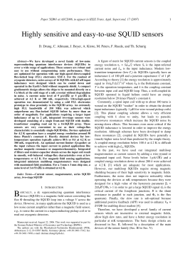
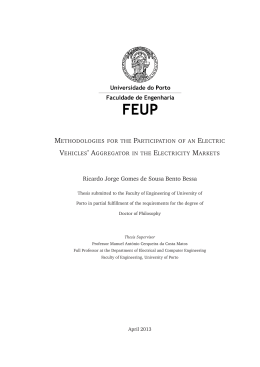
Parameters for PMOSA
To find a good value for the temperature several different constant temperatures
were tested. The experiments were conducted on FON benchmark problem
that was found to be the most challenging of the problems to solve for both
MOEA-RF and PMOSA. The results are presented in figure 1, and based on
the results temperature T = 4 was chosen to be used in the actual experiment.
The selection of temperature was a compromise between best performance on
low levels of noise versus acceptable performance on high levels of noise. Lower
temperatures did provide better convergence with low levels of noise, but higher
temperatures were able to find decent solution with higher probability when the
noise level was high. This suggest that decreasing temperature function could
provide best overall performance in solving FON, but this was not tested in this
study.
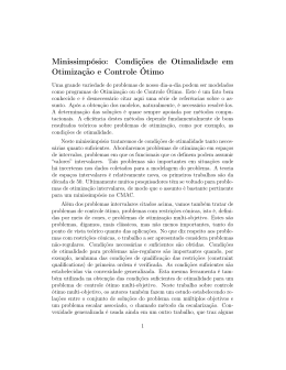
Different methods for generating new solutions with different values of δ were
also tested. The results are presented in figure 2. Some of the tested combinations were worse than others but there were many good combinations and the
selection of best alternative was not clear. Perturbation method that chooses
perturbation for one decision variable at a time from Laplace distribution with
δ = (ximax − ximin )/10 was selected because it produced the highest mean of
hypervolume ratio but the difference was not statistically significant compared
to other methods.
Third parameter that could be modified is the number of samples to evaluate
the objective function. In real world simulation problems evaluation of objective
function is the computationally most expensive part in optimization. Therefore
the number of evaluations is the limiting factor in the running time of the algorithm. We assume that samples are IID and the noise is normally distributed, so
when the number of samples grows large the sample mean approaches the noiseless objective function value and variance of sample mean approaches zero. This
means that with enough samples it is possible to solve a problem with any level
of noise. This leads to trade-off between how many times the objective function
is sampled and how many different solution candidates can be processed during
the algorithm.
The same consideration is valid also for MOEA-RF and the number of samples, L = 10 in PMOSA vs. L = 1 in MOEA-RF, is actually one of the main
differences between the algorithms. It can be observed from the examples in
appendix A that the objective function values are much closer to P Ftrue in
PMOSA executions. The ratio between the
√ magnitudes of visible noise is given
by standard error of the mean and it is 10. This is probably the main result
why PMOSA is able to find better solutions than MOEA-RF to problems with
high levels of noise.
Different trials in altering the sample count in both MOEA-RF and PMOSA
would be interesting to conduct but those were not performed in this study.
4.2
Speed of convergence
50000 evaluations was enough for the algorithms to demonstrate their performance with the given parameters and benchmark problems. The fastest conver-
12
gence in metrics was seen with DTLZ2B problem and slowest with FON with
both MOEA-RF and PMOSA (figures in appendix A: 13, 14, 15, 16, 17, 18).
MOEA-RF was able to find the approximate solutions to problems in less
evaluations than PMOSA, but the gap in the metrics reduces with more evaluations. It should also be noted that unlike MOEA-RF, PMOSA algorithm
always returns the requested number of solutions that are more or less dominated by each other. Therefore the number of found solutions is not a valid
metric in comparisons between MOEA-RF and PMOSA as it is to compare
different MOEAs.
From the figures it can be concluded that with low levels of noise MOEARF converges to the correct solution slightly faster than PMOSA. In FON with
high levels of noise the metrics of PMOSA still seem to be growing at 50000
evaluations so increasing the number of evaluations would probably result in
better solutions. To put it other way, if the number of evaluations is limited
MOEA-RF is able to produce result with similar quality faster.
13
Mean of HVR in found PF
1
Noise 0.1%
Noise 1%
Noise 2%
Noise 5%
Noise 10%
Noise 20%
0.9
0.8
Hypervolume Ratio
0.7
0.6
0.5
0.4
0.3
0.2
0.1
0
0.01
0.1
0.5
1
2
4
6
Temperature
8
10
100
1000
Figure 1 — HVR metric of solution found by PMOSA to FON with different temperatures and different levels of noise. Unlike the other experiments, here archive size
N = 50.
14
Mean and standard deviation of HVR in found PF
1
0.9
0.8
Hypervolume Ratio
0.7
0.6
0.5
0.4
0.3
0.2
0.1
Noise 0.1%
Noise 2%
Noise 10%
0
0
0
/5
/5
1/5
/20
/10
/20
/10
1/2
1/1
+1
+1
+ 1 rm +
+1
+1
+1
ce
e+
e+
m
m
m
m
c
c
a
o
r
r
r
r
l
f
i
o
o
p
ifo
ifo
pla
pla
nif
nif
Un
La
Un
La
Un
La
+U
+ U ll + U ne +
e+
e+
e+
e+
e+
All
A
All
O
On
On
On
On
On
orm
nif
Figure 2 — HVR metric of solution found by PMOSA to FON with different algorithms for generating the new solution from the current solution.
“All” = All components of the decision variable were modified at the same time,
“One” = One component of the decision variable was modified at a time,
“Uniform” = The values were chosen from the uniform distribution,
“Laplace” = The values were chosen from Laplace distribution,
fraction is the size of δ in eq. 23 relative to ximax − ximin .
15
Mean HVR of found PF
1
Hypervolume Ratio
0.8
0.6
0.4
0.2
0
0.1 %
EA & FON
SA & FON
EA & DTLZ2B
SA & DTLZ2B
EA & KUR
SA & KUR
1%
2%
5%
10 %
20 %
10 %
20 %
10 %
20 %
Noise level
Mean GD of found PF
0.35
Generational Distance
0.3
0.25
0.2
0.15
0.1
0.05
0
0.1 %
1%
2%
5%
Noise level
Mean size of found PF
100
90
Pareto front size
80
70
60
50
40
30
20
10
0.1 %
1%
2%
5%
Noise level
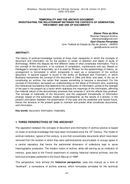
Figure 3 — Mean values of hypervolume ratio (HVR), generational distance (GD)
and number of solution found by MOEA-RF (EA) and PMOSA (SA) optimization
algorithms to test problems FON, DTLZ2B, and KUR with different levels of noise
with 30 repetitions for each combination.
16
4.3
Quality of solutions
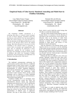
The performance metrics show some differences in response to noise between
MOEA-RF and PMOSA (figure 3). Hypervolume ratio (figure 4) examined
together with spacing metric (figure 5) proved to be to be a good metric to describe the overall quality of the final solution. HVR describes how accurately the
Pareto front was found and S describes how evenly the solutions are distribute
along the Pareto front.
As noted also by Goh and Tan the results of MOEA-RF were slightly better
with low levels of noise compared to test setup with no noise [7]. In PMOSA
algorithm this phenomenon was even stronger. With noise levels less than 2%
both algorithms were able to find the Pareto front of the benchmark problems
equally well, with small exception in PMOSA and FON combination. The
spacing of solutions along the Pareto front was consistently better with PMOSA
than with MOEA-RF. Specially in DTLZ2B the solutions found by MOEA-RF
were concentrated along the middle of the Pareto front as can be seen from
figures 8 and 11 in appendix A.
KUR and DTLZ2B were both easier to solve than FON. With higher levels
of noise both algorithms usually found some solutions but failed to find the
whole Pareto front that is demonstrated by examples of PMOSA algorithm
solving KUR with different levels of noise in figure 12. With KUR problem
the PMOSA algorithm outperformed MOEA-RF with all noise levels. Specially
with 10% and 20% noise PMOSA was still able to find a solutions to KUR and
DTLZ2B with hypervolume ratio near 1, while GA was not. It can be concluded
that with this selection of parameters PMOSA can solve problems with higher
levels of noise than MOEA-RF.
FON proved to be the most difficult of the benchmark problems for both
algorithms to solve. As can be seen in figure 10 the PMOSA algorithm had
some difficulties in escaping the initial solution altogether. However, on average
the results obtained with PMOSA to FON were better that results obtained
with MOEA-RF with high levels of noise. With low levels of noise MOEA-RF
was more accurate. With lower temperature PMOSA would have showed more
similar performance to MOAR-RF, but slightly higher temperature was chosen
to show PMOSA’s ability to handle high levels of noise.
Overall PMOSA produced better quality of solutions compared to MOEARF with all noise levels in KUR and DTLZ2B benchmark problems and with
high noise levels in FON. MOEA-RF was better with FON problem in less noisy
environments.
17
Noise 1 %
1
0.8
0.8
Hypervolume Ratio
Hypervolume Ratio
Noise 0.1 %
1
0.6
0.4
0.6
0.4
0.2
0.2
0
0
B
B
UR
UR
ON
ON
Z2
Z2
TL A & K A & K
& F A & F DTL
S
E
EA
S
&
&D
A
A
E
S
EA
UR
UR
ON Z2B Z2B
ON
& F A & F DTL DTL A & K A & K
E
S
S
&
&
A
A
E
S
Noise 5 %
1
0.8
0.8
Hypervolume Ratio
Hypervolume Ratio
Noise 2 %
1
0.6
0.4
0.2
0.6
0.4
0.2
0
0
B
B
UR
UR
ON
ON
Z2
Z2
TL A & K A & K
& F A & F DTL
S
E
EA
S
&
&D
A
A
E
S
EA
UR
UR
ON Z2B Z2B
ON
& F A & F DTL DTL A & K A & K
E
S
S
&
&
A
A
E
S
Noise 20 %
1
0.8
0.8
Hypervolume Ratio
Hypervolume Ratio
Noise 10 %
1
0.6
0.4
0.2
0.6
0.4
0.2
0
0
B
2B KUR KUR
Z2
LZ
& F A & F DTL
DT EA & SA &
S
EA
&
&
EA
SA
ON
ON
EA
UR
UR
ON Z2B Z2B
ON
& F A & F DTL DTL A & K A & K
E
S
S
&
&
EA
SA
Figure 4 — Hypervolume ratio metric of solutions found by MOEA-RF (EA) and
PMOSA (SA) optimization algorithms to test problems FON, DTLZ2B, and KUR
with different levels of noise with 30 repetitions for each combination. In this box plot
the height of the box and line in the middle describe the upper and lower quartile and
the median of HVR values. The line extending from the box marks the rest of the
data range except for the distant outliers that are drawn as crosses.
18
−4
−4
Noise 0.1 %
x 10
5
5
4
4
Spacing
Spacing
x 10
3
2
1
1
0
0
−3
x 10
EA
UR
UR
ON
ON Z2B Z2B
& F A & F DTL DTL A & K A & K
S
E
S
&
&
EA
SA
−3
Noise 2 %
3
2.5
2.5
2
2
Spacing
Spacing
3
1.5
1
0.5
0.5
0
0
−3
10
x 10
x 10
EA
UR
UR
ON Z2B Z2B
ON
& F A & F DTL DTL A & K A & K
E
S
S
&
&
A
A
E
S
−3
Noise 10 %
10
8
6
6
Spacing
8
4
2
0
0
EA
x 10
Noise 20 %
4
2
B
B
UR
UR
ON
ON
Z2
Z2
TL A & K A & K
& F A & F DTL
EA
S
E
S
&
&D
A
A
E
S
Noise 5 %
1.5
1
B
B
UR
UR
ON
ON
Z2
Z2
TL A & K A & K
& F A & F DTL
S
E
EA
S
&
&D
A
A
E
S
Spacing
3
2
B
2B KUR KUR
ON
ON
Z2
LZ
& F A & F DTL
DT EA & SA &
EA
S
&
&
EA
SA
Noise 1 %
ON FON LZ2B LZ2B KUR KUR
T
T
&
&
&
EA
SA
SA A & D A & D
S
E
&F
Figure 5 — Spacing metric of solutions found by MOEA-RF (EA) and PMOSA (SA)
optimization algorithms to test problems FON, DTLZ2B, and KUR with different
levels of noise with 30 repetitions for each combination. Boxes are drawn as in figure
4
19
PMOSA & FON, noise = 5 %
PMOSA & FON, noise = 5 %
1
f2
f2
1
0.5
0
0.5
0
0
0.5
f1
1
0
PMOSA & FON, noise = 5 %
1
f2
f2
1
PMOSA & FON, noise = 5 %
1
0.5
0
0.5
0
0
0.5
f1
1
0
PMOSA & FON, noise = 5 %
0.5
f1
1
PMOSA & FON, noise = 10 %
1
f2
1
f2
0.5
f1
0.5
0
0.5
0
0
0.5
f1
1
0
0.5
f1
1
Figure 6 — Six examples of PMOSA solution to FON with 5% noise. Found solutions
are drawn as circles, corresponding noiseless objective function values as crosses, and
P Ftrue as continuous line.
20
5
Summary
A reference algorithm MOEA-RF was implemented in this study in order to
compare it with proposed PMOSA algorithm in presence of noise. The performance of implemented MOEA-RF was similar but slightly inferior compared to
the results that were provided by Goh and Tan in [7]. However, the MOEA-RF
algorithm implemented here produced better results than other MOEAs presented by Goh and Tan. Therefore we can conclude that the MOEA-RF that
was implemented is a representative multiobjective evolutionary algorithm that
can be used as a reference point for PMOSA.
It was observed that selecting the optimal parameters for both MOEA and
MOSA requires some work and experimentation and even small changes in algorithm parameters may have clearly observable effect on results. The algorithms
were not separately tuned for the different benchmark problems, but the same
parameters were used for solving all the problems.
For most experiments conducted in this study the PMOSA algorithm performed equally well or better than MOEA-RF algorithm. The only exception
was FON benchmark problem with low levels of noise. This was caused by the
choice of temperature parameter that was tuned towards more noisy problems.
PMOSA by Mattila et al. [6] proved to be very promising algorithm in
solving different kinds of multiobjective optimization problems and further work
on the algorithm is well justified. Introducing adaptive sample count and nonconstant annealing schedule are likely to improve the PMOSA algorithm.
21
References
[1] C. M. Fonseca and P. J. Fleming, “An overview of evolutionary algorithms
in multiobjective optimization,” Evolutionary Computation, vol. 3, pp. 1–
16, 1995.
[2] S. Kirkpatrick, C. D. Gelatt, Jr., and M. P. Vecchi, “Optimization by simulated annealing,” Science, vol. 220, pp. 671–680, 1983.
[3] B. Suman and P. Kumar, “A survey of simulated annealing as a tool for single and multiobjective optimization,” Journal of the Operational Research
Society, vol. 57, pp. 1143–1160, October 2005.
[4] S. Bandyopadhyay, S. Saha, U. Maulik, and K. Deb, “A simulated
annealing-based multiobjective optimization algorithm: Amosa,” Evolutionary Computation, IEEE Transactions on, vol. 12, no. 3, pp. 269–283,
2008.
[5] K. I. Smith, R. M. Everson, J. E. Fieldsend, C. Murphy, and R. Misra,
“Dominance-based multiobjective simulated annealing,” Evolutionary Computation, IEEE Transactions on, vol. 12, no. 3, pp. 323–342, 2008.
[6] V. Mattila, K. Virtanen, and R. P. Hämäläinen, “Scheduling periodic
maintenance of a fighter aircraft fleet using a multi-objective simulationoptimization approach,” tech. rep., Helsinki University of Technology, Systems analysis laboratory, Jun 2009.
[7] C. K. Goh and K. C. Tan, “An investigation on noisy environments in evolutionary multiobjective optimization,” IEEE Transactions on Evolutionary
Computation, no. 3, pp. 354–381, 2007.
[8] M. H. Alrefaei and S. Andradottir, “A Simulated Annealing Algorithm with
Constant Temperature for Discrete Stochastic Optimization,” MANAGEMENT SCIENCE, vol. 45, no. 5, pp. 748–764, 1999.
[9] K. Bryan, P. Cunningham, and N. Bolshakova, “Application of simulated
annealing to the biclustering of gene expression data,” Information Technology in Biomedicine, IEEE Transactions on, vol. 10, pp. 519–525, July
2006.
[10] R. Marion, R. Michel, and C. Faye, “Atmospheric correction of hyperspectral data over dark surfaces via simulated annealing,” Geoscience and Remote Sensing, IEEE Transactions on, vol. 44, pp. 1566–1574, June 2006.
[11] E. Aggelogiannaki and H. Sarimveis, “A simulated annealing algorithm for
prioritized multiobjective optimization – implementation in an adaptive
model predictive control configuration,” Systems, Man, and Cybernetics,
Part B: Cybernetics, IEEE Transactions on, vol. 37, pp. 902–915, Aug.
2007.
[12] K. Deb, “An introduction to genetic algorithms,” tech. rep., Indian Institute
of Technology Kanpur, Kanpur, India, 1997.
22
[13] K. Deb, S. Agrawal, A. Pratap, and T. Meyarivan, “A fast and elitist multiobjective genetic algorithm: Nsga-ii,” IEEE Transactions on Evolutionary
Computation, no. 2, pp. 182–197, 2002.
23
A
Results of all experiments
EA & FON, noise = 0.1 %
EA & FON, noise = 1 %
1
f2
f2
1
0.5
0
0.5
0
0
0.5
f1
1
0
EA & FON, noise = 2 %
1
f2
f2
1
EA & FON, noise = 5 %
1
0.5
0
0.5
0
0
0.5
f1
1
0
EA & FON, noise = 10 %
0.5
f1
1
EA & FON, noise = 20 %
1
f2
1
f2
0.5
f1
0.5
0
0.5
0
0
0.5
f1
1
0
0.5
f1
1
Figure 7 — Examples of MOEA-RF solution to FON with different levels of noise.
Found solutions are drawn as circles, corresponding noiseless objective function values
as crosses, and P Ftrue as continuous line.
24
EA & DTLZ2B, noise = 0.1 %
EA & DTLZ2B, noise = 1 %
1
f2
f2
1
0.5
0
0.5
0
0
0.5
f1
1
0
EA & DTLZ2B, noise = 2 %
1
f2
f2
1
EA & DTLZ2B, noise = 5 %
1
0.5
0
0.5
0
0
0.5
f1
1
0
EA & DTLZ2B, noise = 10 %
0.5
f1
1
EA & DTLZ2B, noise = 20 %
1
f2
1
f2
0.5
f1
0.5
0
0.5
0
0
0.5
f1
1
0
0.5
f1
1
Figure 8 — Examples of MOEA-RF solution to DTLZ2B with different levels of
noise. Symbols as in fig 7.
25
EA & KUR, noise = 0.1 %
EA & KUR, noise = 1 %
−0.5
−0.5
f2
0
f2
0
−1
−1
−2
−1.5
−2
−1.5
f1
f1
EA & KUR, noise = 2 %
EA & KUR, noise = 5 %
−0.5
−0.5
f2
0
f2
0
−1
−1
−2
−1.5
−2
−1.5
f1
f1
EA & KUR, noise = 10 %
EA & KUR, noise = 20 %
−0.5
−0.5
f2
0
f2
0
−1
−1
−2
−1.5
−2
f1
−1.5
f1
Figure 9 — Examples of MOEA-RF solution to KUR with different levels of noise.
Symbols as in fig 7. In reality P Ftrue is disconnect with gaps in places where straight
horizontal line is drawn in in the pictures at f2 = 0 and f2 = −0.45.
26
SA & FON, noise = 0.1 %
SA & FON, noise = 1 %
1
1
0.5
0.5
0
0
0
0.5
1
0
SA & FON, noise = 2 %
1
0.5
0.5
0
0
0.5
1
0
SA & FON, noise = 10 %
1
0.5
0.5
0
0
0.5
0.5
1
SA & FON, noise = 20 %
1
0
1
SA & FON, noise = 5 %
1
0
0.5
1
0
0.5
1
Figure 10 — Examples of PMOSA solution to FON with different levels of noise.
Symbols as in fig 7.
27
SA & DTLZ2B, noise = 0.1 %
SA & DTLZ2B, noise = 1 %
1
1
0.5
0.5
0
0
0
0.5
1
0
SA & DTLZ2B, noise = 2 %
1
0.5
0.5
0
0
0.5
1
0
SA & DTLZ2B, noise = 10 %
1
0.5
0.5
0
0
0.5
0.5
1
SA & DTLZ2B, noise = 20 %
1
0
1
SA & DTLZ2B, noise = 5 %
1
0
0.5
1
0
0.5
1
Figure 11 — Examples of PMOSA solution to DTLZ2B with different levels of noise.
Symbols as in fig 7.
28
SA & KUR, noise = 0.1 %
SA & KUR, noise = 1 %
0
0
−0.5
−0.5
−1
−1
−2
−1.5
−2
SA & KUR, noise = 2 %
SA & KUR, noise = 5 %
0
0
−0.5
−0.5
−1
−1
−2
−1.5
−2
SA & KUR, noise = 10 %
−1.5
SA & KUR, noise = 20 %
0
0
−0.5
−0.5
−1
−1
−2
−1.5
−1.5
−2
−1.5
Figure 12 — Examples of PMOSA solution to KUR with different levels of noise.
Symbols as in fig 7.
29
EA & FON
EA & FON
0.7
1
0.1%
1%
2%
5%
10%
20%
0.6
0.5
0.8
0.6
GD
MS
0.4
0.3
0.4
0.2
0.2
0.1
0
0
1
2
3
evaluations
4
0
5
0
1
4
x 10
EA & FON
2
3
evaluations
4
5
4
x 10
EA & FON
0.018
1
0.016
0.8
0.014
0.012
0.6
S
HVR
0.01
0.008
0.4
0.006
0.004
0.2
0.002
0
0
1
2
3
evaluations
4
0
5
0
1
4
x 10
2
3
evaluations
4
5
4
x 10
Figure 13 — Development of performance metrics over time in MOEA-RF solution
to FON with different levels of noise.
SA & FON
SA & FON
0.7
1
0.1%
1%
2%
5%
10%
20%
0.6
0.5
0.8
0.6
GD
MS
0.4
0.3
0.4
0.2
0.2
0.1
0
0
1
−4
1.4
2
3
evaluations
4
0
5
0
1
4
x 10
SA & FON
x 10
2
3
evaluations
4
5
4
x 10
SA & FON
0.9
0.8
1.2
0.7
1
0.6
S
HVR
0.8
0.6
0.5
0.4
0.3
0.4
0.2
0.2
0
0.1
0
1
2
3
evaluations
4
0
5
4
x 10
0
1
2
3
evaluations
4
5
4
x 10
Figure 14 — Development of performance metrics over time in PMOSA solution to
FON with different levels of noise.
30
EA & DTLZ2B
EA & DTLZ2B
0.35
1.005
0.1%
1%
2%
5%
10%
20%
0.3
0.25
1
0.995
MS
GD
0.2
0.99
0.15
0.985
0.1
0.98
0.05
0
0
1
−3
6
2
3
evaluations
4
5
0.975
0
1
4
x 10
EA & DTLZ2B
x 10
2
3
evaluations
4
5
4
x 10
EA & DTLZ2B
1
0.9
5
0.8
0.7
HVR
S
4
3
0.6
0.5
2
0.4
1
0
0.3
0
1
2
3
evaluations
4
0.2
5
0
1
4
x 10
2
3
evaluations
4
5
4
x 10
Figure 15 — Development of performance metrics over time in MOEA-RF solution
to DTLZ2B with different levels of noise.
SA & DTLZ2B
SA & DTLZ2B
0.4
1
0.1%
1%
2%
5%
10%
20%
0.35
0.3
0.8
0.7
MS
GD
0.25
0.9
0.2
0.6
0.15
0.5
0.1
0.4
0.05
0.3
0
0
1
−3
6
2
3
evaluations
4
0.2
5
0
1
4
x 10
SA & DTLZ2B
x 10
2
3
evaluations
4
5
4
x 10
SA & DTLZ2B
1
5
0.8
4
HVR
S
0.6
3
0.4
2
0.2
1
0
0
1
2
3
evaluations
4
5
4
x 10
0
0
1
2
3
evaluations
4
5
4
x 10
Figure 16 — Development of performance metrics over time in PMOSA solution to
DTLZ2B with different levels of noise.
31
EA & KUR
EA & KUR
0.7
1
0.1%
1%
2%
5%
10%
20%
0.6
0.5
0.9
0.8
GD
MS
0.4
0.7
0.3
0.6
0.2
0.5
0.1
0
0
1
2
3
evaluations
4
0.4
5
0
1
4
x 10
EA & KUR
2
3
evaluations
4
5
4
x 10
EA & KUR
0.035
1
0.9
0.03
0.8
0.025
0.7
S
HVR
0.02
0.015
0.6
0.5
0.4
0.01
0.3
0.005
0
0.2
0
1
2
3
evaluations
4
0.1
5
0
1
4
x 10
2
3
evaluations
4
5
4
x 10
Figure 17 — Development of performance metrics over time in MOEA-RF solution
to KUR with different levels of noise.
SA & KUR
SA & KUR
1.4
1
0.1%
1%
2%
5%
10%
20%
1.2
1
0.9
0.8
MS
GD
0.8
0.7
0.6
0.6
0.4
0.5
0.2
0
0
1
2
3
evaluations
4
0.4
5
0
1
4
x 10
SA & KUR
2
3
evaluations
4
5
4
x 10
SA & KUR
0.014
1
0.012
0.8
0.01
0.6
S
HVR
0.008
0.006
0.4
0.004
0.2
0.002
0
0
1
2
3
evaluations
4
5
4
x 10
0
0
1
2
3
evaluations
4
5
4
x 10
Figure 18 — Development of performance metrics over time in PMOSA solution to
KUR with different levels of noise.
32
B
B.1
Implementation of the benchmark problems
FON.m
function ans = FON(X)
% ans = FON(X)
%
% The FON test problem for multiobjective optimization.
% The row n X(n,:) contains one set of input parameters
% answers (f1,f2) for inputs X(n,1:8) are in ans(n , 1:2).
% Input variable range [-2, 2]
f(:,1) = 1 - exp(-1 * sum((X-(1/sqrt(8))).^2,2));
f(:,2) = 1 - exp(-1 * sum((X+(1/sqrt(8))).^2,2));
B.2
KUR.m
function ans = KUR(X)
% ans = KUR(X)
%
% The KUR test problem for multiobjective optimization.
% The row n X(n,:) contains one set of input parameters
% answers (f1,f2) for inputs X(n,1:3) are in ans(n , 1:2).
% Input variable range [-5, 5]
f(:,1) = (-10 * exp(-0.2 * sqrt(X(:,1).^2 + X(:,2).^2)) - ...
10 * exp(-0.2 * sqrt(X(:,2).^2 + X(:,3).^2))) / 10;
f(:,2) = sum(abs(X).^0.8 + 5 * sin(X.^3),2) / 10;
B.3
DTLZ2B.m
function ans = DTLZ2B(X)
% ans = DTLZ2B(X)
%
% The DTLZ2B test problem for multiobjective optimization.
% The row n X(n,:) contains one set of imput parameters
% answers (f1,f2) for inputs X(n,1:5) are in ans(n , 1:2)
% Input variable range [0, 1]
g = sum((x(:,2:end)-0.5).^2,2);
f= zeros(size(x,1),2);
f(:,1) = cos(x(:,1) .* pi/2) .* (1+g);
f(:,2) = sin(x(:,1) .* pi/2) .* (1+g);
33
C
Implementation of MOEA-RF algorithm
Enhanced Multiobjective Evolutionary Algorithm (MOEA-RF) defined by Goh
and Tan [7].
C.1
moearf.m
function [PF_KNOWN, SOLUTIONS] = moearf(TEST_FUNC, LOWER, UPPER, NOISE)
% [PF_KNOWN, SOLUTIONS] = moearf(TEST_FUNC, LOWER, UPPER, NOISE)
%
% Inputs:
% =======
% TEST_FUNC - function reference to test function like FON
% LOWER
- Lower limits of decision variables. Length of LOWER sets the
%
number of dimensions in decision variables
% UPPER
- Upper limits of decision variables. Size must agree with LOWER
% NOISE
- standard deviation of normally distributed noise
%
% Outputs:
% ========
% PF_FOUND - objective function values of found pareto front
% SOLUTIONS - solutions corresponding rows of PF_FOUND
%---------------------------------% Helper functions
dv_range = max(UPPER) - min(LOWER);
dv_below_zero = -1 * min([0 LOWER]);
gt_bits = 15;
% Convert population matrix from phenotype to genotype
function G = p2g(P)
G = uint32((P + dv_below_zero) ./ dv_range * (2^(gt_bits+1)-1));
end
% Convert population matrix from genotype to phenotype
function P = g2p(G)
P = double(G) ./ (2^(gt_bits+1)-1) .* dv_range - dv_below_zero;
end
% Fix limits. Some optimizations may move phenotypes over genotype rage
function P = enforce_limits(P)
too_low = find(P < repmat(LOWER,size(P,1),1));
too_high = find(P > repmat(UPPER,size(P,1),1));
low = repmat(LOWER,size(P,1),1);
high = repmat(UPPER,size(P,1),1);
P(too_low) = low(too_low);
P(too_high) = high(too_high);
end
%-------------------------------%--------------------------------% Configuration
generations = 500;
p_len = 100;
elite_size = 100;
elite_swap = 10;
mutation_prob = 1/15;
% Noise optimizations on/off
ELDP = 1;
GASS = 1;
34
POSS = 1;
%---------------------------------
%--------------------------------% 1. Initialize
population = unifrnd(repmat(LOWER, p_len, 1), repmat(UPPER,p_len,1));
population_prev = population;
population_prev_prev = population;
pf=[];
pf_solutions=[];
%--------------------------------%--------------------------------% Main Loop
for N = 1:generations
% 2. Evaluate: count noiseless objective function values for population
%
and add noise. Noiseless objective function values are only used to
%
calculate statistics
perf_without_noise = TEST_FUNC(population);
perf = perf_without_noise + normrnd(0, NOISE, size(population,1), 2);
% 2.1 Update Archive. Either use possibilistic archiving model
%
with distance L or pareto ranking
pf = [pf;perf];
pf_solutions = [pf_solutions; population];
if POSS
L = NOISE;
pareto = find_pareto_front_possibilistic(pf,L);
else
pareto = find_pareto_front(pf);
end
pf = pf(pareto,:);
pf_solutions = pf_solutions(pareto,:);
% 2.2 Limit the size of archive by using diversity operator
[pf, pf_solutions] = diversity_operator(pf, pf_solutions, ...
elite_size, 1/p_len);
% 3. Select: Do tournament selection with radomized pairs.
%
Don’t mess up the order of population.
ts_order = randperm(size(perf,1));
winners = tournament_selection(perf,ts_order);
perf = perf(winners,:);
population = population(winners,:);
% 3.1 Replace random members of population with best solutions from
%
the archive
swap = min([elite_swap size(pf_solutions,1) size(population,1)]);
r_pop = randperm(size(population,1));
r_pop = r_pop(1:swap);
r_best = randperm(size(pf_solutions,1));
r_best = r_best(1:swap);
population(r_pop,:) = pf_solutions(r_best,:);
% 4. Crossover
c_order = randperm(size(population,1));
population = crossover(population, c_order, 0.5, @p2g, @g2p);
% 5. Mutate: Either ELDP or plain bitwise
if ELDP
35
% Carry some momentum element-wise from previous generation
d_min = 0.0;
d_max = 0.1;
alpha = 1;
population_prev_prev = population_prev;
population_prev = population;
delta_prev = population_prev - population_prev_prev;
special_mutate = alpha * abs(delta_prev) > d_min & ...
alpha * abs(delta_prev) < d_max;
population = mutate(population, mutation_prob, @p2g, @g2p);
population(special_mutate) = population_prev(special_mutate) + ...
alpha * delta_prev(special_mutate);
population = enforce_limits(population);
else
population = mutate(population, mutation_prob, @p2g, @g2p);
end
if GASS & N > 150
% Gene adaptation to either diverge or converge solutions if necessary
c_limit = 0.6;
d_limit = 0.6;
prob = 1/8;
w = 0.1;
lowbd = min(pf_solutions);
uppbd = max(pf_solutions);
meanbd = mean(pf_solutions);
values_to_change = find(unifrnd(0,1,size(population)) < prob);
for K = 1: size(population,2)
c_values(:,K) = unifrnd(lowbd(K) - w * abs(meanbd(K)), ...
uppbd(K) + w * abs(meanbd(K)), ...
size(population,1), 1);
d_values(:,K) = unifrnd(meanbd(K) - w * abs(meanbd(K)), ...
meanbd(K) + w * abs(meanbd(K)), ...
size(population,1), 1);
end
if size(pf,1) > c_limit * elite_size
population(values_to_change) = c_values(values_to_change);
elseif size(pf,1) < d_limit * elite_size
population(values_to_change) = d_values(values_to_change);
end
population = enforce_limits(population);
end
end
%---------------------------PF_KNOWN = pf;
SOLUTIONS = pf_solutions;
end
C.2
crossover.m
function new_population = crossover(old_population, order, prob, p2g, g2p)
%
% Uniform crossover for MOEA-RF
M = size(old_population,1);
cross_prob = rand(M,1) > prob;
crossover_mask = random_bit_matrix([M, size(old_population,2)], 0.5);
crossover_mask(cross_prob,:) = 0;
bit_population = p2g(old_population);
new_bit_population = zeros(size(bit_population),’uint32’);;
36
for I = 1:2:M-1
x = order([I I+1]);
new_bit_population(x(1),:) = bitand(bit_population(x(1),:), ...
crossover_mask(x(1),:)) + ...
bitand(bit_population(x(2),:), ...
bitcmp(crossover_mask(x(1),:)));
new_bit_population(x(2),:) = bitand(bit_population(x(2),:), ...
crossover_mask(x(1),:)) + ...
bitand(bit_population(x(1),:), ...
bitcmp(crossover_mask(x(1),:)));
end
new_population = g2p(new_bit_population);
end
C.3
mutate.m
function new_population = mutate(old_population, prob, p2g, g2p)
%
% Bitwise mutation for MOEA-RF
% Inputs:
% prob - Probability of mutation for each bit
% p2g - function to convert population phenotype to genotype
% g2p - function to convert population genotype to phenotype
% old_population - Population before mutation in phenotype space
% Output:
% new_population - Population after mutation in phenotype space
bit_population = p2g(old_population);
new_bit_population = bitxor(bit_population, ...
random_bit_matrix(size(bit_population),prob));
new_population = g2p(new_bit_population);
C.4
tournament selection.m
function winners = tournament_selection(perf, pairing)
%
% Tournament selection based on pareto ranking of given matrix of
% performace measures and paring. Row indices of winners are returned.
function ans = x_is_non_dominated(perf_x, perf_y)
ans = all(all(perf_x <= perf_y));
end
M = size(perf,1);
winners = [];
for I = 1:2:M-1
o = pairing([I I+1]);
if x_is_non_dominated(perf(o(1),:), perf(o(2),:))
winners([end+1 end+2]) = [o(1) o(1)];
else
winners([end+1 end+2]) = [o(2) o(2)];
end
end
end
C.5
diversity operator.m
function [PF, solutions] = diversity_operator(PF, solutions, max_count, ...
niche_radius)
% [PF, solutions] = diversity_operator(PF, solutions, max_count, niche_radius)
37
%
% Diversity operator for MOEA-RF. This function performs recurrent
% truncation operation on "PF" so that "max_count" members are left
% in PF and corresponding solutions
while size(PF,1) > max_count
niche_count = sum((squareform(pdist(PF)) + eye(size(PF,1)) * 10 ) < ...
niche_radius);
most_crowded = find(niche_count == max(niche_count));
to_remove = most_crowded(randperm(length(most_crowded)));
to_remove = to_remove(1);
PF(to_remove,:) = [];
solutions(to_remove,:) = [];
end
C.6
find pareto front possibilistic.m
function winners = find_pareto_front_possibilistic(perf, L)
%
% Necessity possiblistic pareto front finding algorithm for MOEA-RF
% Returns the row indices of given objective function
% values that belong to the Pareto set.
%
% NOTE: This function works only for two dimensional objective functions.
len = size(perf,1);
dominated = zeros(len,1);
mask = ones(len,1);
I = 1;
while I < len
mask(I) = 0;
dominated = dominated | ((perf(:,1) - unifrnd(0,L,len,1) >= perf(I,1)) & ...
(perf(:,2) - unifrnd(0,L,len,1) >= perf(I,2))) & mask;
index_not_dominated = (find(not(dominated)));
mask(I) = 1;
I=min([index_not_dominated(index_not_dominated > I) ;len]);
end
winners = find(not(dominated));
C.7
random bit matrix.m
function result = random_bit_matrix(s,prob)
bits = uint32(rand(s(1), s(2), 15) < prob);
result = zeros(s,’uint32’);
for I = 1:15
result = result + bits(:,:,I).*2^(I-1);
end
end
38
D
Implementation of PMOSA algorithm
Probabilistic Multiobjective Simulated Annealing Algorithm (PMOSA) defined
and originally implemented by Mattila et.al [6]. This algorithm is modified to
accept different benchmark problems.
D.1
sa2ba.m
function [S,P,fo] = sa2ba(noise, rstate,r,M,T,gamma, TEST_FUNC, LOWER, UPPER)
%Simulated annealing for test problem dtlz2 with uncertainty
%
% PMOSA algorithm - additive version
% a maximum of gamma solutions are included in the non-dominated set
%Initialization------------------------d=size(LOWER,2);
%
%
l=LOWER;
%
u=UPPER;
%
V=[noise^2 noise^2];
%
delta=(max(UPPER) - min(LOWER))/10;
%
%
%r=10;
%
%T=2;
%
%gamma=3;
%
%
%
less than gamma
fo=[];
fout=0;
cout=0;
%Initialization-end---------------------
Dimension of the vector of decision
variables
Lower bounds of decision variables
Upper bounds
Variances of objective function values
Amount of change in generating
new solutions
Number of samples to evaluate objectives
Temperature
Insert into non-dominated set, if
probability of being dominated is
%Initial solution----------------------k=1;
%rand(’state’,rstate);
x=unifrnd(l,u);
y=x;
fi=TEST_FUNC(x);
%
%
%
%
Random state for initial solution
Initial solution
Store
Actual objective function values
e1=normrnd(0,sqrt(V(1)),1,r);
e2=normrnd(0,sqrt(V(2)),1,r);
% Uncertainties
f=[mean(fi(1)+e1) mean(fi(2)+e2)];
v=[var(fi(1)+e1)/r var(fi(2)+e2)/r];
% estimated ofvs
% variance estimates of means
fx=f;
vx=v;
% Store
px=0;
py=px;
% Probability that x is dominated by
%
the current S
% Store
p=1;
P=0;
% Acceptance probability
% Mutual probabilities of domination
acc=1;
ins=1;
% Accept as current solution
% Insert into non-dominated set
S=[x fx vx];
Sn=1;
% Currently selected non-dominated set
% Size of S
39
%Initial solution-end------------------%Iteratation---------------------------while k<M
k=k+1;
%Generate new candidate solution
y=gen(x,delta,l,u);
%Evaluate
fi=TEST_FUNC(y);
e1=normrnd(0,sqrt(V(1)),1,r);
e2=normrnd(0,sqrt(V(2)),1,r);
f=[mean(fi(1)+e1) mean(fi(2)+e2)];
v=[var(fi(1)+e1)/r var(fi(2)+e2)/r];
I=find(ismember(S(:,1:d),x,’rows’));
% Actual objective function values
% Uncertainties
% estimated ofvs
% variance estimates of means
% Position of x in S
%Determine energy of x as probability of being dominated by S and y
if isempty(I)
% x is not in S
px=0;
for i=1:size(S,1)
px=px+pdom(S(i,d+1:d+2),S(i,d+3:d+4),fx,vx);
end
else
% x is in S
px=sum(P(I,:));
end
px=px+pdom(f,v,fx,vx);
% Account for y
%Determine energy of y as probability of being dominated by S and x
py=0;
for i=1:size(S,1)
py=py+pdom(S(i,d+1:d+2),S(i,d+3:d+4),f,v);
end
%Insertion into non-dominated set
if Sn<gamma || py<max(sum(P,2))
ins=1;
else
ins=0;
end
%Remove the most dominated element if the size of S exceeds gamma
if ins==1 && Sn==gamma
[z,I2]=max(sum(P,2));
I3=[1:I2-1 I2+1:Sn];
S=S(I3,:);
P=P(I3,I3);
Sn=Sn-1;
end
%Update probabilities of being dominated within S
if ins==1;
S(end+1,:)=[y f v];
Sn=Sn+1;
P(Sn,Sn)=0;
%Probability that y dominates y
for i=1:Sn-1
%Probability that y dominates ith member of S
P(i,Sn)=pdom(S(Sn,d+1:d+2),S(Sn,d+3:d+4),S(i,d+1:d+2),S(i,d+3:d+4));
%Probability that ith member of S dominates i
P(Sn,i)=pdom(S(i,d+1:d+2),S(i,d+3:d+4),S(Sn,d+1:d+2),S(Sn,d+3:d+4));
40
end
end
%Acceptance of y
if isempty(I)
py=py+pdom(fx,vx,f,v);
end
%x is not in S
%Account for x
acc=0;
if py<=px
acc=1;
p=1;
else
p=exp(-(py-px)/T);
if rand<=p
acc=1;
end
end
%If accepted, set current solution,
if acc==1
x=y;
fx=f;
vx=v;
end
%Command line output
if cout
fprintf(’k: %2d
f1: %4.3f
f2: %4.3f
px: %4.3f
py: %4.3f’ ...
’p: %4.3f acc: %1d
ins: %1d
#S: %2d \n’, ...
k,f(1),f(2),px,py,p,acc,ins,size(S,1));
end
%Save values
if fout
fo(end+1,:)=[px py];
end
end
%Iteratation end------------------------
D.2
gen.m
function f=gen(x,d,l,u)
%
%
%
%
Generate new solution from x
l
lower bounds
u
upper bounds
Laplace distribution - one element perturbed
k=unidrnd(length(x));
x(k)=x(k)+laprnd(d);
f=x;
%Restore feasibility
if f(k)<l(k)
f(k)=2*l(k)-f(k);
elseif f(k)>u(k)
f(k)=2*u(k)-f(k);
end
41
D.3
pdom.m
function f=pdom(x1,s1,x2,s2)
%Probability that design 1 dominates design 2 in context of minimization
%x1,x2 vector of estimates for epected objective function values
%s1,s2 vector of variance estimates
%Obervations of ofvs assumed normally distributed
f=prod(normcdf(0,x1-x2,sqrt(s1+s2)));
D.4
laprnd.m
function x=laprnd(b)
% Generates Laplace distributed random variates with
% location parameter equal to 0
% scale parameter equal to b
[m,n]=size(b);
u=unifrnd(-1/2,1/2,m,n);
x=-b.*sign(u).*log(1-2*abs(u));
42
E
Implementation of metrics
Performance metrics defined by Goh and Tan [7].
E.1
stats.m
function [GD, MS, S, HVR] = stats(pf_known, pf_true)
%
% Scalar performace metrics GD, MS, S, and HVR between two
% sets of two vectors of two dimensional objective function values.
% GD - Generational Distance
klen=size(pf_known,1);
tlen=size(pf_true,1);
fcount=size(pf_true,2);
gdsum = 0;
for I = 1:klen
gdsum = gdsum + min(sum( (pf_true - repmat(pf_known(I,:),tlen,1)).^2,2));
end
GD = sqrt(gdsum / klen);
% MS - Maximum Spread
mssum = 0;
for I = 1:fcount
mssum = mssum + ((min(max(pf_known(:,I)), max(pf_true(:,I))) - ...
max(min(pf_known(:,I)), min(pf_true(:,I)))) / ...
(max(pf_true(:,I)) - min(pf_true(:,I))))^2;
end
MS = sqrt(mssum / fcount);
% S - Spacing
distances = squareform(pdist(pf_known));
distances = distances + eye(size(distances)) * 10;
min_distances = min(distances);
d_avg = mean(min_distances);
ssum = sum((min_distances-d_avg).^2);
S = sqrt(ssum / klen) / klen;
% HVR - Hypervolume Ratio
% Volume objective space that is dominated by pareto front.
% Calculated by creating a grid of zeros that fills the objective space
% and then going through the pareto fronts and setting all grid points to 1
% that are dominated by pareto points
if size(pf_known,2) == 2
grid_points = combvec(min(pf_true(:,1)):0.01:max(pf_true(:,1)), ...
min(pf_true(:,2)):0.01:max(pf_true(:,2)))’;
grid_known = zeros(size(grid_points));
grid_true = zeros(size(grid_points));
for I = 1 : size(pf_known,1);
grid_known(find(all([grid_points(:,1) >= pf_known(I,1), ...
grid_points(:,2) >= pf_known(I,2)],2)),:) = 1;
end
for I = 1 : size(pf_true,1);
grid_true(find(all([grid_points(:,1) >= pf_true(I,1), ...
grid_points(:,2) >= pf_true(I,2)],2)),:) = 1;
end
HV_known = sum(sum(grid_known));
HV_true = sum(sum(grid_true));
HVR = HV_known / HV_true;
else
HVR = 0;
end
end
43