An Evolving Fuzzy-GARCH Approach for Financial Volatility Modeling and
Forecasting
Leandro S. Maciel† , Fernando Gomide† , Rosangela Ballini‡
†
Departamento de Engenharia de Computação e Automação Industrial - DCA
Faculdade de Engenharia Elétrica e de Computação - FEEC
Universidade Estadual de Campinas - UNICAMP
Av. Albert Einstein 400, 13.083-852, Campinas, São Paulo, Brasil
Emails: {maciel,gomide}@dca.fee.unicamp.br
‡
Departamento de Teoria Econômica - DTE
Instituto de Economia - IE
Universidade Estadual de Campinas - UNICAMP
Rua Pitágoras 353, 13.083-857, Campinas, São Paulo, Brasil
Email: [email protected]
Abstract
Volatility forecasting is a challenging task that has attracted the attention of market practitioners, regulators and academics in recent years. This paper proposes an evolving fuzzyGARCH approach to model and forecast the volatility of S&P 500 and Ibovespa indexes.
The model comprises both the concept of evolving fuzzy systems and GARCH modeling
approach in order to consider the principles of time-varying volatility and volatility clustering, in which changes are cataloged by similarity. Evolving fuzzy systems use data streams
to continuously adapt the structure and functionality of fuzzy models to improve their performance, which is computationally efficient. The results show the high potential of the evolving
fuzzy-GARCH model to forecast stock returns volatility, outperforming GARCH-type models
in statistical terms.
Keywords: Artificial intelligence, Risk analysis, Forecasting, Evolving systems, Volatility.
Resumo
Recentemente, a previsão da volatilidade tem atraı́do a atenção de agentes de mercado,
reguladores e acadêmicos. Neste artigo é proposto um modelo GARCH-nebuloso evolutivo
para a modelagem e previsão da volatilidade dos ı́ndices S&P 500 e Ibovespa. O modelo
combina os conceitos de sistemas nebulosos evolutivos e modelos GARCH para considerar os princı́pios de volatilidade variante no tempo e agrupamentos de volatilidade, em
que mudanças no padrão são capturadas por similaridade. Sistemas nebulosos evolutivos
utilizam fluxos de dados para adaptar continuamente a estrutura e funcionalidade de modelos nebulosos funcionais para melhorar o desempenho, caracterizando uma abordagem
computacionalmente eficiente. Os resultados mostraram o elevado potencial do modelo
GARCH-nebuloso evolutivo para a previsão da volatilidade dos retornos dos ı́ndices considerados, superando modelos da familı́a GARCH em termos estatı́sticos.
Palavras-Chave: Inteligência Artificial, Análise de riscos, Previsão, Sistemas evolutivos,
Volatilidade.
Área ANPEC: Área 7 - Microeconomia, Métodos Quantitativos e Finanças
Classificação JEL: C53, C45, G17.
1
1
Introduction
Accurately measuring and forecasting financial volatility plays a crucial role for asset and
derivative pricing, hedge strategies, portfolio allocation and risk management. Since the
1987 stock market crash, academics, practitioners and regulators have been investigated
the development of financial time-series models with changing variance over time in order
to avoid huge investments losses due to their exposure to unexpected market movements
(Bellini & Figà-Talamanca 2005, Charles 2010, Brandão, Dyer & Hahn 2012, Lin, Chen &
Gerlach 2012).
Financial time-series volatility is often characterized by some stylized facts such as volatility clusters, persistence, leptokurtic data behavior and time-varying volatility. A convenient
framework for dealing with time dependent volatility in financial markets concerns the autoregressive conditional heteroskedasticity (ARCH) model, proposed by (Engle 1982), becoming
a popular tool for volatility modeling. Providing a more flexible structure, (Bollerslev 1986)
introduced the Generalized ARCH (GARCH) model, which combines the ARCH and autoregressive moving average (ARMA) models. The GARCH model estimates jointly a conditional
mean and conditional variance equation, and it is characterized by a fat tail and excess of
kurtosis, regularly used in studying the daily returns of stock market data (Han & Park 2008)1 .
Besides the theoretical appeal and empirical evidence in favor to GARCH-family models,
they do not provide mechanisms to deal with volatility clustering.
Methods based on artificial intelligence have been extensively applied as a flexible way to
describe complex dynamics of various economic and financial problems (Haofei, Guoping,
Fangting & Han 2007). (Hamid & Iqbal 2004) suggested the use of an artificial neural network (ANN) model to predict the volatility of S&P 500 index futures prices. (Bildirici & Ersin
2009) enhanced GARCH-family models with ANN to forecast the volatility of daily returns
in Istanbul Stock Exchange. On the other hand, (Hajizadeh, Seifi, Zarandi & Turksen 2012)
proposed a scheme in which the estimates of volatility obtained by an EGARCH model are
fed forward to an ANN model, considering the S&P 500 index prices.
A radial basis function neural network with Gaussian activation functions and robust clustering algorithms to model the conditional volatility of the Spanish electricity pool prices was
suggested by (Coelho & Santos 2011). The authors showed that their model performed better than traditional linear models to predict upward and downward movements in electricity
future prices. Concerning the issue of derivative securities pricing, (Wang 2009) integrated
a GJR-GARCH model into an ANN option-pricing model and indicated that their approach
provides higher predictability than other volatility methodologies. Providing similar results,
(Wang, Lin, Huang & Wu 2012) and (Tseng, Cheng, Wang & Peng 2008) also evaluated
volatility forecasting performance in option pricing combining neural networks and GARCHfamily models.
(Tino, Schittenkopf & Dorffner 2001) introduced a recurrent neural network model to simulate daily trading of straddles on financial indexes based on predictions of daily volatility.
The authors showed that while GARCH models cannot generate any significantly positive
profit, the use of recurrent networks can generate a statistically significant excess profit.
Moreover, (Tung & Quek 2011) jointed a self-organising neural network and option straddle1
Several distinctive approaches have also been conducted for modeling and forecasting financial volatility,
including realized volatility models (Hansen & Lunde 2006) and stochastic volatility (Fouque, Papanicolaou &
Sircar 2000).
2
based approach to financial volatility trading. Compared with several benchmarks, the proposed methodology demonstrated that its ability to forecast the future volatility enhances
investments profits. Despite the high ability to deal with the problem of volatility forecasting,
ANN drawbacks include its “black box” nature, greater computational burden, proneness to
overfitting, and the empirical nature of model development.
Due to these shortcomings, models based on fuzzy theory appear as an alternative
methodology to evaluate high nonlinear systems (Zadeh 2005, Savran 2007). (Popov &
Bykhanov 2005) combined the concept of fuzzy rules and GARCH approach to model volatility of financial time series. The conditional volatility forecasting of foreign exchange rates
returns was considered by (Geng & Ma 2008), using a functional fuzzy inference system
applied to the GARCH model. (Hung 2009a) adopted the method of fuzzy logic systems to
modify the threshold values for an asymmetric GARCH model. Based on simulations, the author showed that the forecasting performance is significantly improved if the leverage effect
of clustering is considered along with the use of fuzzy systems and GARCH approaches.
(Thavaneswaran, Appadoo & Paseka 2009) proposed a fuzzy weighted possibilistic model
for option valuation based on the estimation and forecasting of financial volatility, considered
as fuzzy numbers. They stated that fuzzy assumptions are more flexible and reveal promising results for option pricing as an intuitive way to look at the uncertainty in the models
parameters. To capture the volatility conditional distribution on higher-order moments such
as skewness, a GARCH-Fuzzy-Density method for volatility density forecasting was proposed by (Helin & Koivisto 2011). The model provided more accurate density forecasts for
the higher-order moment varying processes than traditional GARCH models.
Combining the concepts of fuzzy systems and artificial neural networks, (Chang, Wei &
Cheng 2011) suggested the use of a hybrid adaptive network-based fuzzy inference system
(ANFIS) to forecast the volatility of the Taiwan stock market. The authors indicated that the
proposed model is superior to other methods with regard to error measures. Furthermore,
(Luna & Ballini 2012) introduced an adaptive fuzzy system to forecast financial time series
volatility and compared their method with a GARCH model. The results indicate the higher
performance of the adaptive fuzzy approach for volatility forecasting purposes.
A hybrid Fuzzy-GARCH model was suggested by (Hung 2009b). The model comprises a
functional fuzzy inference system with a GARCH model, optimized using a genetic algorithm
framework. Similarly, (Hung 2011a) and (Hung 2011b) proposed a fuzzy system method to
analyze clustering in GARCH models using genetic algorithms and particle swarm optimization to estimate the parameters, respectively. The author indicates that the model offers
significant improvements in forecasting stock market volatility, outperforming some GARCHfamily models.
Therefore, this paper proposes an evolving fuzzy-GARCH approach for financial timeseries volatility modeling and forecasting. The model is based on a collection of fuzzy rules
in the form of IF-THEN statements, in which its structure comprises a GARCH model and
also the evolving fuzzy modeling idea, that uses data streams to continuously adapt the
structure and functionality, ensuring high generality. Here, the rule base, rules membership
functions and consequent parameters continually evolve by adding new rules with higher
summarization power, modifying existing rules and parameters to match current knowledge
(Angelov 2010). Computational experiments illustrating the effectiveness of the proposed
model are provided by modeling and forecasting the volatility of S&P 500 (United States) and
Ibovespa (Brazil) indexes from January 3, 2000 through September 30, 2011, in comparison
3
with some GARCH-family models.
The evolving fuzzy-GARCH model has novel features in comparison to the existing approaches in the literature. First, the proposed method combines a fuzzy scheme with a
GARCH model, providing a more realistic framework that captures both time-varying volatility and volatility clustering. And second, it performs forecasts recursively from flows of data,
which is computational more efficient.
After this briefly introduction, the paper proceeds as follows. Section 2 presents the
evolving fuzzy-GARCH model proposed. Computational experiments and results analysis
for stock market volatility forecasting are reported in Section 3. Next, Section 4 concludes
the paper and suggests issues for further investigation.
2
2.1
Evolving Fuzzy-GARCH Modeling
GARCH-type models
The Generalized Autoregressive Conditional Heteroskedasticity (GARCH) model considers the current conditional variance dependent on the p past conditional variances as well
as the q past squared innovations. Let rt = 100 × (ln Pt − ln Pt−1 ) denote the continuously
compounded rate of stock returns from time t − 1 to t, where Pt is the daily closing stock
price at time t. The GARCH(p, q) model can be written as:
(1)
rt = σt ξt
σt2
=ω+
q
X
2
αi rt−n
+
n=1
p
X
2
βj σt−j
(2)
j=1
where ξt is a sequence of independent and identically distributed (i.i.d.) random variables
with zero-mean and unit variance, σt2 is the conditional variance of ξt , and ω, αn and βj are
unknown coefficients to be estimated.
The GARCH model reduces the number of parameters required by considering the in2
formation in the lag(s) of the conditional variance in addition to the lagged rt−n
term(s) as in
ARCH-type models. GARCH models’ simplicity and ability to capture persistence of volatility
explain its empirical and theoretical appeal. However, it fails to capture stock fluctuations with
volatility clustering well. This fact can lead to poor adequacy and forecast ability. Therefore,
the proposal of a fuzzy-GARCH approach appears as a potential tool for volatility modeling
and forecasting in a presence of volatility clustering.
2.2
The Evolving Fuzzy-GARCH Model
Fuzzy inference systems are universal approximations that can estimate nonlinear continuous functions uniformly with arbitrary accuracy (Ji, Massanari, Ager, Yen, Miller & Ying
2007). Besides the GARCH model considers time-varying volatility, a fuzzy approach provides the capability to simulate stock fluctuations with volatility clustering. The proposed
fuzzy-GARCH model is described by a collection of fuzzy rules in the form of IF-THEN statements in order to describe the stock market fluctuations via a GARCH model. Therefore, the
ith rule of the fuzzy-GARCH(p, q) is written as:
4
2
Ri : IF rt−n is Λi,n AND σt−j
is Λi,q+j
p
q
X
X
2
2
2
βi,j σt−j
αi,n rt−n +
THEN σi,t = ωi +
n=1
(3)
j=1
where Λi,l is the ith fuzzy set (membership function) to describe the stock market return r
and volatility σ 2 (for i = 1, 2, . . . , R, and l = 1, 2, . . . , q + p), R is the number of fuzzy rules,
2
are the previous value of the stock market’s returns and volatility, respectively,
rt−n and σt−j
for n = 1, 2, . . . , q and j = 1, 2, . . . , p.
2
2
2
Let us define x = [rt−1 , rt−2 , . . . , rt−q , σt−1
, σt−2
, . . . , σt−p
]T = [x]Tl the input data vector,
x ∈ <q+p and l = 1, 2, . . . , q + p, and y = σt2 the model output, y ∈ <. Then, the evolving
fuzzy-GARCH assumes antecedent fuzzy sets with Gaussian membership functions:
2
−
µi,l (xl ) = e
(x∗i,l −xl )
(4)
2%2
where µi,l denotes the membership degree of input xl , x∗i,l is the focal point of the lth fuzzy
set of the ith fuzzy rule, and % is the projection of the zone of influence of the ith cluster on
the axis of the lth input variable.
The firing level of the ith rule, assuming the product T -norm of the antecedent fuzzy sets
is:
πi (x) =
q+p
Y
(5)
µi,l (xl )
l=1
The model output y is found as the weighted average of the individual rule contributions:
y=
R
X
i=1
γi yi =
R
X
πi
γi xTe Ψi , γi = PR
h=1
i=1
πh
(6)
T
is the expanded data
where γi is the normalized firing level of the ith rule, xe = 1 xT
T
vector, and Ψi = [ωi , αi,1 , αi,2 , . . . , αi,q , βi,1 , βi,2 , . . . , βi,p ] is the vector of parameters of the ith
linear consequent.
There are essentially two sub-tasks related to the problem of the recursively identification
of the evolving fuzzy-GARCH model: learning the antecedents to determine the focal points
of the rules, and identification the parameters of the linear consequents. These sub-tasks
are described as follows.
2.2.1
Learning Antecedents
The learning procedure applied in fuzzy-GARCH model is the eClustering algorithm,
proposed by (Angelov 2010), which considers streaming data, collected continuously2 . This
mechanism ensures that the new data reinforce and confirm the information contained in
previous data. In off-line situations, the learning procedure can be viewed as a recursive
2
Alternative clustering algorithms for evolving fuzzy models include the ones based on potential or scattering
(Angelov & Filev 2004) and participatory learning (Yager 1990).
5
mechanism to process data. The judgment related to form a new rule or to modify an existing
one is take considering the density at a data point using Cauchy functions.
The density is evaluated recursively and information related to the spatial distribution of
all data, at step k, is accumulated by variables ϕk e δlk as follows:
Dk z k =
(k − 1)
Pq+p
k 2
l=1 (zl )
k−1
P
k k
+ 1 + ϕk − 2 q+p
l=1 zj δj
(7)
where Dk z k is the density of the data around the last data point of the data stream provided
k
T
T T k
to the algorithm,
input/output pair at step k (k = 2, 3, . . .), ϕk =
Pq+p k−1 z2 =1 ([x , ky ] )k−1is ank−1
k−1
ϕ
+ l=1 (zl ) , ϕ = 0, δl = δl + zl and δl1 = 0.
This clustering mechanism ensures a gradual change of the rule-base. Data points with
high density are potential candidates to became focal points of antecedents of fuzzy rules.
The density of a data point selected to be a cluster focal point have its density calculated
by Equation (7) and is updated according to new information available, since any data point
coming from the data stream will influence the data density. Therefore, the focal points
density is recursively updated by:
Dk z i
∗
k−1
=
k − 1 + (k − 2)
1
Dk−1 (z i∗ )
Pq+p i∗
− 1 + l=1
zl − zlk
(8)
∗
where D1 z i = 1, k = 2, 3, . . ., and i∗ denotes the focal points of the ith fuzzy rule. It must
∗
be noted that the initialization (k = 1) includes: z 1 ← z 1 , R ← 1, i.e. the first data point is
considered as a cluster center, forming the first rule.
The recursive density estimation clustering approach does not rely on user- or problemspecific thresholds, differently as in methods like subtractive clustering or participatory learning, for example. Moreover, the density is evaluated recursively and the whole information
that concerns the spatial distribution of all data is accumulated in a small number of variables
(Angelov 2010).
In the eClustering procedure, representative clusters with high generalization capability
are formed considering the data points with the highest value of D. Therefore, the Condition
(I) is formulated:
R
∗
∗
R
(I) : IF Dk z k > max Dk z i OR Dk z k < min Dk z i
i=1
THEN z
(R+1)∗
←z
i=1
k
AND R ← R + 1
(9)
If a current data point satisfies Condition (I) then the new data point is accepted as a
∗
new center and a new rule is formed with focal point based on the new data point (z (R+1) =
z k ; R ← R+1). This condition ensures good convergence, but it is more sensitive to outliers.
Influence of outliers can be avoided using quality clusters indicators (Angelov 2010).
To control the level of overlap and to avoid redundant clusters, Condition (II) is also
considered:
(II) : IF ∃ i : µi,l (xkl ) > e−1 ∀ l
∗
THEN z i is removed AND R ← R − 1
6
(10)
Condition (II) remove highly overlapping clusters, avoiding contradictory rules, which
means that the new candidate cluster focal point describes any of the existing cluster focal
points. The previously existing focal point(s) for which this condition holds is(are) removed.
These mechanisms simplify the rule-base and the number of rules grow according to the
system information availability only.
Quality measures for recursive monitoring the clusters include support, age, utility, zone
of influence and local density (Angelov 2010). Here in this paper, similarly as in (Angelov
2010), the quality of the clusters are constantly monitored using the accumulated relative
firing level of a particular antecedent:
Pk
γt
k
(11)
Ui = t=1 i∗ , i = 1, 2, . . . , R; k = 2, 3, . . .
k−T
∗
where T i denotes the time tag which indicates when the ith fuzzy rule is generated.
The utility of the clusters is evaluated according to the Condition (III):
(III) : IF Uik < ε
∗
THEN z i is removed AND R ← R − 1
(12)
where ε is a threshold related to the minimum utility of a cluster (typically, threshold values
are in the range [0.03, 0.1]) (Angelov 2010).
This condition means that if some cluster has low utility (lower than an threshold ε), the
data pattern has shifted away from the focal point of that rule, then the rule that satisfies
Condition (III) is removed. This quality measure evaluates the importance of the fuzzy rules
and assists the evolving process. The next step is the learning process of consequent
parameters.
2.2.2
Recursive Consequent Parameters Identification
Equation (6) can be put into the following vector form:
y = ΓT Φ
(13)
T
where y is the output, Γ = γ1 xTe , γ2 xTe , . . . , γq+p xTe denotes the fuzzily weighted extended
T
input vector, and Φ = ΨT1 , ΨT2 , . . . , ΨTR the vector of parameters of the rule base.
Since at each step the real/target output is given, the parameters of the consequents
can be updated using the recursive least squares algorithm RLS (Ljung 1988) considering
locally or globally optimization. In this paper we apply a locally optimal error criterion which
is given by:
min ELi
= min
k
X
γi (xt ) y t − (xte )T Ψti
2
(14)
t=1
In the model there are not only fuzzily coupled linear subsystems and streaming data,
but also structure evolution. Thus, the optimal update of the parameters of the ith rule is:
Ψk+1
= Ψki + Σki xke γik y k − (xke )T Ψki , Ψ1i = 0
i
7
(15)
Σk+1
= Σki −
i
γik Σki xke (xke )T Σki
, Σ1i = ΩI(q+p+1)×(q+p+1)
k
k k
k
T
1 + γi (xe ) Σi xe
(16)
where I is a (q+p+1)×(q+p+1) identity matrix, Ω denotes a large number, usually Ω = 1000,
and Σ a dispersion matrix. (Angelov 2010) performed simulations on several benchmarks
and verified the stability and convergence of the RLS updating formulas (15) and (16).
When a new fuzzy rule is added, a new dispersion matrix is computed ΣkR+1 = IΩ.
Parameters of the new rules are approximated from the parameters of the existing R fuzzy
rules as follows:
ΨkR+1
=
R
X
γi Ψk−1
i
(17)
i=1
Otherwise, parameters of all other rules are inherited from the previous step, while the
dispersion matrices are updated independently.
However, when a focal points is replaced by another rule due to Condition (II), the parameters and the dispersion matrix are inherited by the fuzzy rule being replaced:
k
−1
ΨkR+1 = Ψk−1
i∗ , µi∗ ,l (xl ) > e , ∀ l, l = 1, 2, . . . , q + p
(18)
ΣkR+1 = Σik−1
, µi∗ ,l (xkl ) > e−1 , ∀ l, l = 1, 2, . . . , q + p
∗
(19)
Finally, once the consequent parameters are found, the model output is computed using
Equation (6). Therefore, the control parameters are: % (clusters zone of influence) and ε
(utility threshold).
3
Computational Results and Analysis
To illustrate the performance of the proposed evolving fuzzy-GARCH model for modeling and forecasting stock market volatility, this paper focus on daily prices of S&P 500 (US)
and Ibovespa (Brazil) over the period from January 3, 2000 through September 30, 2011,
in comparison with GARCH (Bollerslev 1986), EGARCH (Nelson 1991) and GJR-GARCH
(Glosten, Jagannathan & Runkle 1993) models. The daily stock return series were generated by taking the natural logarithm difference of the daily stock index and the previous
day’s stock index and multiplied by 100. The data sample was partitioned into two parts.
The in-sample period consists on data from January 3, 2000 through December 29, 2005. On
the other hand, the forecast out-of-sample period is from January 2, 2006 through September 30, 2011. This procedure is only necessary for GARCH-type models, since the evolving
fuzzy-GARCH performs on-line, recursively, which does not require a training step.
Table 1 shows the basic statistical characteristics of the return series. The average daily
returns are negative for S&P 500 and positive for Ibovespa. The daily returns display evidence of skewness and kurtosis.
The returns series are skewed towards the left, characterized by a distribution with tails
that are significantly thicker than for a normal distribution. J-B test statistics further confirms
that the daily returns are non-normal distributed. As compared with Gaussian distribution,
8
the kurtosis in S&P 500 and Ibovespa suggest that their daily returns have fat-tailed (Table 1). Ibovespa index has a higher kurtosis than S&P 500, which explains the fact that
emerging countries show in general a more leptokurtic behavior. Under the null hypothesis of no serial correlation in the squared returns, the Ljung-Box Q2 (10) statistics infer a
linear dependence for both series considered. Furthermore, the Engle’s ARCH test for the
squared returns reveals strong ARCH effects, which evidences in support of GARCH effects
(i.e., heteroscedasticity). Accordingly, these preliminary analyses of the data encourage
the adoption of a sophisticated model, which embody fat-tailed features, and of conditional
models to allow for time-varying volatility.
Tab. 1: Descriptive statistics of daily returns of S&P 500 and Ibovespa.
S&P 500
Ibovespa
Mean
−0.0073
0.0378
Max
10.9572
13.6766
Min
−9.4695
−12.0961
Std. Dev.
1.3787
1.9493
Skewness
−0.1580
−0.1066
Excess Kurtosis
3.6701
7.4814
a
∗
J-B
234.9483
277.1270∗
2
b
∗
Q (10)
789.7362
683.9531∗
ARCH Test (10)c 1109.1934∗
1082.7409∗
a
is the statistics of Jarque-Bera normal distribution test.
is the Ljung-Box Q test for the 10th order serial
correlation of the squared returns.
c
Engle’s ARCH test also examines for autocorrelation
of the squared returns.
∗
Significantly at 5%.
b
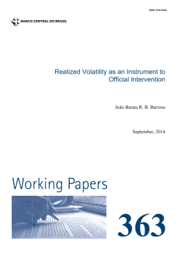
Despite GARCH-type models are able to capture fat-tails and conditional volatility, they
do not consider volatility clustering, as characterized by (Fama 1965). The stock indexes
are shown in Figure 1, and its correspondent returns are given in Figure 2. Particularly, in
Figure 2 the context of volatility clustering became more clear, mainly when the context of
the recent US Subprime crisis is considered.
9
S&P 500
1600
Index
1400
1200
1000
800
Jan 2000
Sept 2003
Sept 2007
Sept 2011
Sept 2007
Sept 2011
Time (in days)
Ibovespa
80,000
Index
60,000
40,000
20,000
Jan 2000
Sept 2003
Time (in days)
Fig. 1: Daily closing stock price indexes for S&P 500 and Ibovespa.
S&P 500
Daily Return (%)
15
10
5
0
−5
Jan 2000
Sept 2003
Sept 2007
Sept 2011
Sept 2007
Sept 2011
Time (in days)
Ibovespa
Daily Return (%)
15
10
5
0
−5
−10
Jan 2000
Sept 2003
Time (in days)
Fig. 2: S&P 500 and Ibovespa daily returns.
In order to select best lag parameters for the evolving fuzzy-GARCH and GARCH-type
specifications, also considered in this work, the Bayesian information criterion (BIC) and
Akaike’s information criterion (AIC) were performed (Akaike 1974, Schwarz 1978). The
models with various combinations of (p, q) parameters ranging from (1, 1) to (15, 15) were
10
calibrated on return data. According to BIC and AIC criteria the best specification for all
volatility models was (1, 1), i.e. p = 1 and q = 1.
Simulations were conducted to chose appropriate control parameters for the fuzzy-GARCH
model, according to different values for these parameters and compared in terms of accuracy. For both indexes, the value of the control parameters are % = 0.05 and ε = 0.13 .
Volatility forecasts comparison was conducted for one-step ahead horizon in terms of
mean squared forecast error (MSFE), mean absolute forecast error (MAFE), and mean percentage forecast error (MPFE) defined as follows:
MSFE =
N
2
1 X 2
σi − σ̂i2
N i=1
(20)
N
1 X 2
|σi − σ̂i2 |
MAFE =
N i=1
(21)
N
1 X |σi2 − σ̂i2 |
MPFE =
N i=1
σi2
(22)
where N is the number of out-of-sample observations, σi2 is the actual volatility at forecasting
period i, measured as the squared daily return, and σ̂i2 is the forecast volatility at i.
Table 2 provides the performance of the evaluated models to predict the S&P 500 and
Ibovespa stock indexes volatilities. The evolving fuzzy-GARCH model performs better than
all remaining models since their structure provides a combination of rules for estimating forecast errors and also a mechanism to deal with volatility clustering. Moreover, the distinctive
GARCH-type models provide similar results.
Tab. 2: Models performance to volatility forecasting for one-step ahead.
Index
Model
MSFE
MAFE
MPFE
S&P 500
Fuzzy-GARCH
0.2017
0.3980
0.4099
GARCH
0.5704
0.7076
0.8366
EGARCH
0.5733
0.7199
0.8422
GJR-GARCH
0.5839
0.7298
0.8420
Ibovespa
Fuzzy-GARCH
0.8552
0.9020
0.3877
GARCH
1.4487
1.2403
0.6723
EGARCH
1.4300
1.2611
0.6831
GJR-GARCH
1.4230
1.1955
0.6511
Although all performance measures of forecasting accuracy that have been extensively
employed in practice, they do not reveal whether the forecast of a model is statistically superior to another one. Therefore, it is imperative to use additional tests to help comparison
among two or more competing models in terms of forecasting accuracy.
This paper adopts the parametric Morgan-Granger-Newbold (MGN) test, initially proposed by (Diebold & Mariano 1995). This test is often employed when the assumption of
3
The parameters of GARCH, EGARCH and GJR-GARCH models were estimated using the traditional maximum likelihood method, which the log-likelihood function is computed from the product of all conditional densities of the prediction residuals.
11
contemporaneous correlation of errors is relaxed. The statistic for this test can be computed
using:
MGN = ρ̂sd
1−ρ̂2sd
N −1
(23)
12
where ρ̂sd is the estimated correlation coefficient between s = e1 + e2 , and d = e1 − e2 , with
e1 and e2 the residuals of two models adjusted, e.g. fuzzy-GARCH model versus GARCHfamily approaches. In this case, the statistic is distributed as Student distribution with N − 1
degrees of freedom, and N is the number of out-of-sample observations. For this test, if the
estimates are equally accurate (null hypothesis), then the correlation between s and d will
be zero.
The results from MGN test, shown in Table 3, are in line with our results. MGN statistics
reveal that the evolving fuzzy-GARCH model is superior predictor for forecasting S&P 500
and Ibovespa indexes than traditional GARCH-type models. The GARCH-family models can
also be considered as equally accurate.
Tab. 3: MGN Statistics for volatility forecast for S&P 500 and Ibovespa.
S&P 500
GARCH
EGARCH
GJR-GARCH
Fuzzy-GARCH
3.8746
3.7262
3.6552
(0.0001)
(0.0002)
(0.0002)
GARCH
–
–
1.5233
(0.1279)
1.6180
(0.1058)
EGARCH
–
–
–
–
1.5534
(0.1205)
Fuzzy-GARCH
GARCH
Ibovespa
GARCH
EGARCH
3.3337
3.4653
(0.0008)
(0.0005)
–
–
1.3299
(0.1837)
GJR-GARCH
3.3928
(0.0007)
1.6253
(0.1043)
EGARCH
–
–
1.5938
–
–
(0.1112)
The relevant p-values are shown in beneath each test statistic
in parenthesis.
Finally, Figure 3 reports the evolution of the number of fuzzy rules in the evolving fuzzyGARCH model. The rule number evolution are similar in both markets, however the S&P
500 showed a more varying structure. It shows the continuous model structure adaptation
through changes in the rule base structure. It is interesting to note that the number of rules
12
increases significantly between 2008 and 2009, revealing the capability of evolving fuzzyGARCH to capture crises instabilities. This period corresponds to the US subprime mortgage crisis which has led to plunging property prices, a slowdown in the US economy, and
billions in banks losses, affecting the main financial markets over the world, Brazil included.
S&P 500
7
# of rules
6
5
4
3
2
1
Jan 2000
Sept 2003
Sept 2007
Sept 2011
Sept 2007
Sept 2011
Time (in days)
Ibovespa
7
# of rules
6
5
4
3
2
1
Jan 2000
Sept 2003
Time (in days)
Fig. 3: Evolution of the number of rules for S&P 500 and Ibovespa indexes.
The proposed model exhibits high capability to forecasting volatility of the real market
returns evaluated by considering both stock market asymmetry and volatility clustering,
also overperforms GARCH, EGARCH and GJR-GARCH methodologies in statistical terms.
Moreover, including the concept of adaptive modeling, the evolving fuzzy-GARCH provides
a more efficient algorithm performing on-line, which is essential for actual decision making
instances as volatility forecasting.
4
Conclusion
Volatility forecasting plays a central role in several financial applications like asset allocation and hedging, option pricing and risk analysis. In this paper, an evolving fuzzy-GARCH
model for financial volatility modeling and forecasting was proposed. It combines both evolving fuzzy systems and the conditional variance GARCH model to deal with stylized facts
such as time-varying volatility and volatility clustering. Since volatility mirrors the behavior
of nonstationary nonlinear environments, evolving models have shown to be quite suitable
to capture its behavior. Empirical evidence based on S&P 500 and Ibovespa indexes market data illustrated the potential of the evolving fuzzy-GARCH approach to the problem of
volatility forecasting, providing more accurate results than GARCH-type models in statistical
terms. This includes periods with high instabilities such as the recent subprime mortgage
crisis. Future works shall include applications of the evolving fuzzy-GARCH model in finan13
cial decision making problems related to volatility such as option pricing, portfolio selection
and risk modeling.
References
Akaike, H. (1974). A new look at the statistical model identification, IEEE Transactions on
Automatic Control 19: 716–723.
Angelov, P. (2010). Evolving Systems: Methodology and Applications, John Wiley & Sons,
Inc., Hoboken, NJ, USA, chapter Evolving Takagi-Sugeno fuzzy systems from streaming
data (eTS+), pp. 21–50.
Angelov, P. & Filev, D. (2004). An approach to online identification of Takagi-Sugeno fuzzy
models, IEEE Transactions on Systems, Man, and Cybernetics – Part B: Cybernetics
4: 484–498.
Bellini, F. & Figà-Talamanca, G. (2005). Runs tests for assessing volatility forecastibility in
financial time series, European Journal of Operational Research 163(1): 102–114.
Bildirici, M. & Ersin, O. O. (2009). Improving forecasts of GARCH family models with the
artificial neural networks: An application to the daily returns in Istanbul Stock Market
Exchange, Expert Systems with Applications 36: 7355–7362.
Bollerslev, T. (1986). Generalized autoregressive conditional heteroskedasticity, Journal of
Econometrics 31: 307–327.
Brandão, L. E., Dyer, J. S. & Hahn, W. J. (2012). Volatility estimation for stochastic project
value models, European Journal of Operational Research 220(3): 642–648.
Chang, J., Wei, L. & Cheng, C. (2011). A hybrid ANFIS model based on AR and volatility for
TAIEX forecasting, Applied Soft Computing 11: 1388–1395.
Charles, A. (2010). The day-of-the-week effects on the volatility: The role of the asymmetry,
European Journal of Operational Research 202(1): 143–152.
Coelho, L. S. & Santos, A. A. P. (2011). A RBF neural network model with GARCH errors:
Application to electricity price forecasting, Eletric Power Systems Research 81: 74–83.
Diebold, F. X. & Mariano, R. S. (1995). Comparing predictive accuracy, Journal of Business
and Economic Statistics 13: 253–265.
Engle, R. F. (1982). Autoregressive conditional heteroskedasticity with estimates of the variance of United Kingdom inflation, Econometrica 50: 987–1007.
Fama, E. F. (1965). he behavior of stock market price, Journal of Business 38: 34–105.
Fouque, J., Papanicolaou, G. & Sircar, R. (2000). Mean reverting stochastic volatility, International Journal of Theoretical and Applied Finance 3: 101–142.
14
Geng, L. & Ma, J. (2008). TSK fuzzy inference system based GARCH model for forecasting
exchange rate volatility, Annals of the Fifty International Conference on Fuzzy Systems
and Knowledge Discovery.
Glosten, L. R., Jagannathan, R. & Runkle, D. E. (1993). On the relation between the expected value and the volatility of the nominal excess return on stocks, Journal of Finance 48: 1779–1801.
Hajizadeh, E., Seifi, A., Zarandi, M. H. F. & Turksen, B. (2012). A hybrid modeling approach
for forecasting the volatility of S&P 500 index return, Expert Systems with Applications
39: 431–436.
Hamid, S. A. & Iqbal, Z. (2004). Using neural networks for forecasting volatility of S&P 500,
Journal of Business Research 57: 1116–1125.
Han, H. & Park, J. Y. (2008). Time series properties of ARCH processes with persistent
covariates, Journal of Econometrics 146: 275–292.
Hansen, P. R. & Lunde, A. (2006). Realized variance and market microstructure noise (with
discussion), Journal of Business and Economic Statistics 24: 127–161.
Haofei, Z., Guoping, X., Fangting, Y. & Han, Y. (2007). A neural network model based on
the multi-stage optimization approach for short-term food pricing forecasting in China,
Expert Systems with Applications 33: 347–356.
Helin, T. & Koivisto, H. (2011). The GARCH-FuzzyDensity method for density forecasting,
Applied Soft Computing 11: 4212–4225.
Hung, J. (2009a). A fuzzy asymmetric GARCH model applied to stock markets, Information
Sciences 179: 3930–3943.
Hung, J. (2009b). A fuzzy GARCH model applied to stock market scenario using a genetic
algorithm, Expert Systems with Applications 36: 11710–11717.
Hung, J. (2011a). Adaptive Fuzzy-GARCH model applied to forecasting the volatility of stock
markets using particle swarm optimization, Information Sciences 181: 4673–4683.
Hung, J. (2011b). Applying a combined fuzzy systems and GARCH model to adaptively
forecast stock market volatility, Applied Soft Computing 11: 3938–3845.
Ji, Y., Massanari, R. M., Ager, J., Yen, J., Miller, R. E. & Ying, H. (2007). A fuzzy logic-based
computational recognition-primed decision model, Information Sciences 177: 4338–
4353.
Lin, E. M. H., Chen, C. W. S. & Gerlach, R. (2012). Forecasting volatility with asymmetric smooth transition dynamic range models, International Journal of Forecasting
28(2): 384–399.
Ljung, L. (1988). System Identification, Theory for the User, Englewood Cliffs, Prentice-Hall,
NJ, USA.
15
Luna, I. & Ballini, R. (2012). Adaptive fuzzy system to forecast financial time series volatility,
Journal of Intelligent & Fuzzy Systems 23: 27–38.
Nelson, D. B. (1991). Conditional heteroskedasticity in asset returns: A new approach,
Econometrica 59: 347–370.
Popov, A. A. & Bykhanov, K. V. (2005). Modeling volatility of time series using fuzzy GARCH
models, Annals of the 9th Russian-Korean International Symposium on Science and
Technology.
Savran, A. (2007). An adaptive recurrent fuzzy system for nonlinear identification, Applied
Soft Computing 7: 593–600.
Schwarz, G. (1978). Estimating the dimension of model, The Annuals of Statistics 6: 461–
464.
Thavaneswaran, A., Appadoo, S. & Paseka, A. (2009). Weighted possibilistic moments of
fuzzy numbers with applications to GARCH modeling and option pricing, Mathematical
and Computer Modeling 49: 352–368.
Tino, P., Schittenkopf, C. & Dorffner, G. (2001). Financial volatility trading using recurrent
neural networks, IEEE Transactions on Neural Networks 12: 865–874.
Tseng, C., Cheng, S., Wang, Y. & Peng, J. (2008). Artificial neural network model of the
hybrid EGARCH volatility of the Taiwan stock index option prices, Physica A: Statistical
Mechanisms and its Applications 387: 3192–3200.
Tung, W. L. & Quek, C. (2011). Financial volatility trading using a self-organising neural-fuzzy
semantic network and option straddle-based approach, Expert Systems with Applications 38: 4668–4688.
Wang, C., Lin, S., Huang, H. & Wu, P. (2012). Using neural network for forecasting TXO price
under different volatility models, Expert Systems with Applications 39: 5025–5032.
Wang, Y. (2009). Nonlinear neural network forecasting model for stock index option price:
Hybrid GJR-GARCH approach, Expert Systems with Applications 36: 564–570.
Yager, R. (1990). A model of participatory learning, IEEE Transactions on Systems, Man
and Cybernetics 20: 1229–1234.
Zadeh, L. (2005). Toward a generalized theory of uncertainty (GTU) - An outline, Information
Sciences 172: 1–40.
16