Nonlinear physics
(solitons, chaos, discrete breathers)
N. Theodorakopoulos
Konstanz, June 2006
Contents
Foreword
vi
1 Background: Hamiltonian mechanics
1.1 Lagrangian formulation of dynamics . . . . . . . . . . . . . .
1.2 Hamiltonian dynamics . . . . . . . . . . . . . . . . . . . . . .
1.2.1 Canonical momenta . . . . . . . . . . . . . . . . . . .
1.2.2 Poisson brackets . . . . . . . . . . . . . . . . . . . . .
1.2.3 Equations of motion . . . . . . . . . . . . . . . . . . .
1.2.4 Canonical transformations . . . . . . . . . . . . . . . .
1.2.5 Point transformations . . . . . . . . . . . . . . . . . .
1.3 Hamilton-Jacobi theory . . . . . . . . . . . . . . . . . . . . .
1.3.1 Hamilton-Jacobi equation . . . . . . . . . . . . . . . .
1.3.2 Relationship to action . . . . . . . . . . . . . . . . . .
1.3.3 Conservative systems . . . . . . . . . . . . . . . . . . .
1.3.4 Separation of variables . . . . . . . . . . . . . . . . . .
1.3.5 Periodic motion. Action-angle variables . . . . . . . .
1.3.6 Complete integrability . . . . . . . . . . . . . . . . . .
1.4 Symmetries and conservation laws . . . . . . . . . . . . . . .
1.4.1 Homogeneity of time . . . . . . . . . . . . . . . . . . .
1.4.2 Homogeneity of space . . . . . . . . . . . . . . . . . .
1.4.3 Galilei invariance . . . . . . . . . . . . . . . . . . . . .
1.4.4 Isotropy of space (rotational symmetry of Lagrangian)
1.5 Continuum field theories . . . . . . . . . . . . . . . . . . . . .
1.5.1 Lagrangian field theories in 1+1 dimensions . . . . . .
1.5.2 Symmetries and conservation laws . . . . . . . . . . .
1.6 Perturbations of integrable systems . . . . . . . . . . . . . . .
.
.
.
.
.
.
.
.
.
.
.
.
.
.
.
.
.
.
.
.
.
.
.
.
.
.
.
.
.
.
.
.
.
.
.
.
.
.
.
.
.
.
.
.
.
.
.
.
.
.
.
.
.
.
.
.
.
.
.
.
.
.
.
.
.
.
.
.
.
.
.
.
.
.
.
.
.
.
.
.
.
.
.
.
.
.
.
.
.
.
.
.
.
.
.
.
.
.
.
.
.
.
.
.
.
.
.
.
.
.
.
.
.
.
.
.
.
.
.
.
.
.
.
.
.
.
.
.
.
.
.
.
.
.
.
.
.
.
.
.
.
.
.
.
.
.
.
.
.
.
.
.
.
.
.
.
.
.
.
.
.
.
.
.
.
.
.
.
.
.
.
.
.
.
.
.
.
.
.
.
.
.
.
.
.
.
.
.
.
.
.
.
.
.
.
.
.
.
.
.
.
.
.
.
.
.
.
1
1
1
1
2
2
2
3
3
3
4
4
5
5
6
6
7
7
7
7
8
8
8
9
2 Background: Statistical mechanics
2.1 Scope . . . . . . . . . . . . . . .
2.2 Formulation . . . . . . . . . . . .
2.2.1 Phase space . . . . . . . .
2.2.2 Liouville’s theorem . . . .
2.2.3 Averaging over time . . .
2.2.4 Ensemble averaging . . .
2.2.5 Equivalence of ensembles
2.2.6 Ergodicity . . . . . . . . .
.
.
.
.
.
.
.
.
.
.
.
.
.
.
.
.
.
.
.
.
.
.
.
.
.
.
.
.
.
.
.
.
.
.
.
.
.
.
.
.
.
.
.
.
.
.
.
.
.
.
.
.
.
.
.
.
.
.
.
.
.
.
.
.
.
.
.
.
.
.
.
.
11
11
11
11
12
12
12
13
13
FPU paradox
The harmonic crystal: dynamics . . . . . . . . . . . . . . . . . . . . . . . . .
The harmonic crystal: thermodynamics . . . . . . . . . . . . . . . . . . . . .
The FPU numerical experiment . . . . . . . . . . . . . . . . . . . . . . . . . .
15
15
16
17
3 The
3.1
3.2
3.3
.
.
.
.
.
.
.
.
.
.
.
.
.
.
.
.
i
.
.
.
.
.
.
.
.
.
.
.
.
.
.
.
.
.
.
.
.
.
.
.
.
.
.
.
.
.
.
.
.
.
.
.
.
.
.
.
.
.
.
.
.
.
.
.
.
.
.
.
.
.
.
.
.
.
.
.
.
.
.
.
.
.
.
.
.
.
.
.
.
.
.
.
.
.
.
.
.
.
.
.
.
.
.
.
.
.
.
.
.
.
.
.
.
.
.
.
.
.
.
.
.
.
.
.
.
.
.
.
.
Contents
4 The Korteweg - de Vries equation
4.1 Shallow water waves . . . . . . . . . . . . . . . . . . .
4.1.1 Background: hydrodynamics . . . . . . . . . .
4.1.2 Statement of the problem; boundary conditions
4.1.3 Satisfying the bottom boundary condition . . .
4.1.4 Euler equation at top boundary . . . . . . . . .
4.1.5 A solitary wave . . . . . . . . . . . . . . . . . .
4.1.6 Is the solitary wave a physical solution? . . . .
4.2 KdV as a limiting case of anharmonic lattice dynamics
4.3 KdV as a field theory . . . . . . . . . . . . . . . . . .
4.3.1 KdV Lagrangian . . . . . . . . . . . . . . . . .
4.3.2 Symmetries and conserved quantities . . . . . .
4.3.3 KdV as a Hamiltonian field theory . . . . . . .
.
.
.
.
.
.
.
.
.
.
.
.
.
.
.
.
.
.
.
.
.
.
.
.
.
.
.
.
.
.
.
.
.
.
.
.
.
.
.
.
.
.
.
.
.
.
.
.
.
.
.
.
.
.
.
.
.
.
.
.
.
.
.
.
.
.
.
.
.
.
.
.
.
.
.
.
.
.
.
.
.
.
.
.
.
.
.
.
.
.
.
.
.
.
.
.
.
.
.
.
.
.
.
.
.
.
.
.
.
.
.
.
.
.
.
.
.
.
.
.
.
.
.
.
.
.
.
.
.
.
.
.
.
.
.
.
.
.
.
.
.
.
.
.
.
.
.
.
.
.
.
.
.
.
.
.
20
20
20
21
21
22
23
24
24
25
25
26
27
5 Solving KdV by inverse scattering
5.1 Isospectral property . . . . . . . . . . . . . . . . . . . . . . . . . . . . . . . .
5.2 Lax pairs . . . . . . . . . . . . . . . . . . . . . . . . . . . . . . . . . . . . . .
5.3 Inverse scattering transform: the idea . . . . . . . . . . . . . . . . . . . . . .
5.4 The inverse scattering transform . . . . . . . . . . . . . . . . . . . . . . . . .
5.4.1 The direct problem . . . . . . . . . . . . . . . . . . . . . . . . . . . . .
5.4.2 Time evolution of scattering data . . . . . . . . . . . . . . . . . . . . .
5.4.3 Reconstructing the potential from scattering data (inverse scattering
problem) . . . . . . . . . . . . . . . . . . . . . . . . . . . . . . . . . .
5.4.4 IST summary . . . . . . . . . . . . . . . . . . . . . . . . . . . . . . . .
5.5 Application of the IST: reflectionless potentials . . . . . . . . . . . . . . . . .
5.5.1 A single bound state . . . . . . . . . . . . . . . . . . . . . . . . . . . .
5.5.2 Multiple bound states . . . . . . . . . . . . . . . . . . . . . . . . . . .
5.6 Integrals of motion . . . . . . . . . . . . . . . . . . . . . . . . . . . . . . . . .
5.6.1 Lemma: a useful representation of a(k) . . . . . . . . . . . . . . . . .
5.6.2 Asymptotic expansions of a(k) . . . . . . . . . . . . . . . . . . . . . .
5.6.3 IST as a canonical transformation to action-angle variables . . . . . .
28
28
28
29
29
29
31
6 Solitons in anharmonic lattice dynamics:
6.1 The model . . . . . . . . . . . . . . .
6.2 The dual lattice . . . . . . . . . . . .
6.2.1 A pulse soliton . . . . . . . .
6.3 Complete integrability . . . . . . . .
6.4 Thermodynamics . . . . . . . . . . .
42
42
43
44
45
46
the Toda
. . . . . .
. . . . . .
. . . . . .
. . . . . .
. . . . . .
lattice
. . . .
. . . .
. . . .
. . . .
. . . .
7 Chaos in low dimensional systems
7.1 Visualization of simple dynamical systems . . . . .
7.1.1 Two dimensional phase space . . . . . . . .
7.1.2 4-dimensional phase space . . . . . . . . . .
7.1.3 3-dimensional phase space; nonautonomous
of freedom . . . . . . . . . . . . . . . . . . .
7.2 Small denominators revisited: KAM theorem . . .
7.3 Chaos in area preserving maps . . . . . . . . . . .
7.3.1 Twist maps . . . . . . . . . . . . . . . . . .
7.3.2 Local stability properties . . . . . . . . . .
7.3.3 Poincaré-Birkhoff theorem . . . . . . . . . .
7.3.4 Chaos diagnostics . . . . . . . . . . . . . .
7.3.5 The standard map . . . . . . . . . . . . . .
7.3.6 The Arnold cat map . . . . . . . . . . . . .
7.3.7 The baker map; Bernoulli shifts . . . . . . .
ii
.
.
.
.
.
.
.
.
.
.
.
.
.
.
.
.
.
.
.
.
.
.
.
.
.
.
.
.
.
.
.
.
.
.
.
.
.
.
.
.
. . . . . . . . . .
. . . . . . . . . .
. . . . . . . . . .
systems with one
. . . . . . . . . .
. . . . . . . . . .
. . . . . . . . . .
. . . . . . . . . .
. . . . . . . . . .
. . . . . . . . . .
. . . . . . . . . .
. . . . . . . . . .
. . . . . . . . . .
. . . . . . . . . .
.
.
.
.
.
.
.
.
.
.
.
.
.
.
.
.
.
.
.
.
.
.
.
.
.
. . . . .
. . . . .
. . . . .
degree
. . . . .
. . . . .
. . . . .
. . . . .
. . . . .
. . . . .
. . . . .
. . . . .
. . . . .
. . . . .
32
34
35
35
36
39
39
39
41
48
48
48
50
51
52
53
53
54
55
55
58
63
64
Contents
7.4
7.3.8 The circle map. Frequency locking . . . . . . . . . . . . . . . . . . . . 66
Topology of chaos: stable and unstable manifolds, homoclinic points . . . . . 67
8 Solitons in scalar field theories
8.1 Definitions and notation . . . . . . . . . . . .
8.1.1 Lagrangian, continuum field equations
8.2 Static localized solutions (general KG class) .
8.2.1 General properties . . . . . . . . . . .
8.2.2 Specific potentials . . . . . . . . . . .
8.2.3 Intrinsic Properties of kinks . . . . . .
8.2.4 Linear stability of kinks . . . . . . . .
8.3 Special properties of the SG field . . . . . . .
8.3.1 The Sine-Gordon breather . . . . . . .
8.3.2 Complete Integrability . . . . . . . . .
.
.
.
.
.
.
.
.
.
.
.
.
.
.
.
.
.
.
.
.
.
.
.
.
.
.
.
.
.
.
.
.
.
.
.
.
.
.
.
.
.
.
.
.
.
.
.
.
.
.
.
.
.
.
.
.
.
.
.
.
.
.
.
.
.
.
.
.
.
.
.
.
.
.
.
.
.
.
.
.
.
.
.
.
.
.
.
.
.
.
.
.
.
.
.
.
.
.
.
.
.
.
.
.
.
.
.
.
.
.
.
.
.
.
.
.
.
.
.
.
.
.
.
.
.
.
.
.
.
.
9 Atoms on substrates: the Frenkel-Kontorova model
9.1 The Commensurate-Incommensurate transition . . . . . . . . . . . .
9.1.1 The continuum approximation . . . . . . . . . . . . . . . . .
9.1.2 The special case ² = 0: kinks and antikinks . . . . . . . . . .
9.1.3 The general case ² > 0: the soliton lattice . . . . . . . . . . .
9.2 Breaking of analyticity . . . . . . . . . . . . . . . . . . . . . . . . . .
9.2.1 FK ground state as minimizing periodic orbit of the standard
9.2.2 Small amplitude motion . . . . . . . . . . . . . . . . . . . . .
9.2.3 Free end boundary conditions . . . . . . . . . . . . . . . . . .
9.3 Metastable states: spatial chaos as a model of glassy structure . . .
.
.
.
.
.
.
.
.
.
.
.
.
.
.
.
.
.
.
.
.
.
.
.
.
.
.
.
.
.
.
69
69
69
71
71
72
73
74
75
75
76
. . .
. . .
. . .
. . .
. . .
map
. . .
. . .
. . .
.
.
.
.
.
.
.
.
.
.
.
.
.
.
.
.
.
.
77
78
78
79
79
83
84
85
85
86
.
.
.
.
.
.
.
.
.
.
.
.
.
.
.
.
.
.
.
.
10 Solitons in magnetic chains
10.1 Introduction . . . . . . . . . . . . . . . . . . . . . . . . . . . . .
10.2 Classical spin dynamics . . . . . . . . . . . . . . . . . . . . . .
10.2.1 Spin Poisson brackets . . . . . . . . . . . . . . . . . . .
10.2.2 An alternative representation . . . . . . . . . . . . . . .
10.3 Solitons in ferromagnetic chains . . . . . . . . . . . . . . . . . .
10.3.1 The continuum approximation . . . . . . . . . . . . . .
10.3.2 The classical, isotropic, ferromagnetic chain . . . . . . .
10.3.3 The easy-plane ferromagnetic chain in an external field
10.4 Solitons in antiferromagnets . . . . . . . . . . . . . . . . . . . .
10.4.1 Continuum dynamics . . . . . . . . . . . . . . . . . . . .
10.4.2 The isotropic antiferromagnetic chain . . . . . . . . . .
10.4.3 Easy axis anisotropy . . . . . . . . . . . . . . . . . . . .
10.4.4 Easy plane anisotropy . . . . . . . . . . . . . . . . . . .
10.4.5 Easy plane anisotropy and symmetry-breaking field . . .
.
.
.
.
.
.
.
.
.
.
.
.
.
.
.
.
.
.
.
.
.
.
.
.
.
.
.
.
.
.
.
.
.
.
.
.
.
.
.
.
.
.
.
.
.
.
.
.
.
.
.
.
.
.
.
.
.
.
.
.
.
.
.
.
.
.
.
.
.
.
.
.
.
.
.
.
.
.
.
.
.
.
.
.
.
.
.
.
.
.
.
.
.
.
.
.
.
.
.
.
.
.
.
.
.
.
.
.
.
.
.
.
88
88
88
88
89
90
90
91
96
99
99
101
102
105
106
11 Solitons in conducting polymers
11.1 Peierls instability . . . . . . . . . . . . . . . . .
11.1.1 Electrons decoupled from the lattice . .
11.1.2 Electron-phonon coupling; dimerization
11.2 Solitons and polarons in (CH)x . . . . . . . . .
11.2.1 A continuum approximation . . . . . . .
11.2.2 Dimerization . . . . . . . . . . . . . . .
11.2.3 The soliton . . . . . . . . . . . . . . . .
11.2.4 The polaron . . . . . . . . . . . . . . . .
.
.
.
.
.
.
.
.
.
.
.
.
.
.
.
.
.
.
.
.
.
.
.
.
.
.
.
.
.
.
.
.
.
.
.
.
.
.
.
.
.
.
.
.
.
.
.
.
.
.
.
.
.
.
.
.
.
.
.
.
.
.
.
.
110
110
110
111
114
114
116
117
119
iii
.
.
.
.
.
.
.
.
.
.
.
.
.
.
.
.
.
.
.
.
.
.
.
.
.
.
.
.
.
.
.
.
.
.
.
.
.
.
.
.
.
.
.
.
.
.
.
.
.
.
.
.
.
.
.
.
.
.
.
.
.
.
.
.
.
.
.
.
.
.
.
.
Contents
12 Solitons in nonlinear optics
12.1 Background: Interaction of light with matter, Maxwell-Bloch equations . . .
12.1.1 Semiclassical theoretical framework and notation . . . . . . . . . . . .
12.1.2 Dynamics . . . . . . . . . . . . . . . . . . . . . . . . . . . . . . . . . .
12.2 Propagation at resonance. Self-induced transparency . . . . . . . . . . . . . .
12.2.1 Slow modulation of the optical wave . . . . . . . . . . . . . . . . . . .
12.2.2 Further simplifications: Self-induced transparency . . . . . . . . . . .
12.3 Self-focusing off-resonance. . . . . . . . . . . . . . . . . . . . . . . . . . . . .
12.3.1 Off-resonance limit of the MB equations . . . . . . . . . . . . . . . . .
12.3.2 Nonlinear terms . . . . . . . . . . . . . . . . . . . . . . . . . . . . . .
12.3.3 Space-time dependence of the modulation: the nonlinear Schrödinger
equation . . . . . . . . . . . . . . . . . . . . . . . . . . . . . . . . . . .
12.3.4 Soliton solutions . . . . . . . . . . . . . . . . . . . . . . . . . . . . . .
122
122
122
123
123
123
125
126
126
127
128
129
13 Solitons in Bose-Einstein Condensates
132
13.1 The Gross-Pitaevskii equation . . . . . . . . . . . . . . . . . . . . . . . . . . . 132
13.2 Propagating solutions. Dark solitons . . . . . . . . . . . . . . . . . . . . . . . 132
14 Unbinding the double helix
14.1 A nonlinear lattice dynamics approach . . . . . . . . .
14.1.1 Mesoscopic modeling of DNA . . . . . . . . . .
14.1.2 Thermodynamics . . . . . . . . . . . . . . . . .
14.2 Nonlinear structures (domain walls) and DNA melting
14.2.1 Local equilibria . . . . . . . . . . . . . . . . . .
14.2.2 Thermodynamics of domain walls . . . . . . . .
.
.
.
.
.
.
.
.
.
.
.
.
.
.
.
.
.
.
.
.
.
.
.
.
.
.
.
.
.
.
.
.
.
.
.
.
134
134
134
135
139
140
142
15 Pulse propagation in nerve cells: the Hodgkin-Huxley model
15.1 Background . . . . . . . . . . . . . . . . . . . . . . . . . . . . . . . .
15.2 The Hodgkin-Huxley model . . . . . . . . . . . . . . . . . . . . . . .
15.2.1 The axon membrane as an array of electrical circuit elements
15.2.2 Ion transport via distinct ionic channels . . . . . . . . . . . .
15.2.3 Voltage clamping . . . . . . . . . . . . . . . . . . . . . . . . .
15.2.4 Ionic channels controlled by gates . . . . . . . . . . . . . . . .
15.2.5 Membrane activation is a threshold phenomenon . . . . . . .
15.2.6 A qualitative picture of ion transport during nerve activation
15.2.7 Pulse propagation . . . . . . . . . . . . . . . . . . . . . . . .
.
.
.
.
.
.
.
.
.
.
.
.
.
.
.
.
.
.
.
.
.
.
.
.
.
.
.
.
.
.
.
.
.
.
.
.
.
.
.
.
.
.
.
.
.
144
144
144
145
146
146
146
148
148
148
.
.
.
.
.
.
.
.
.
.
151
151
151
151
152
152
153
153
153
153
155
.
.
.
.
.
.
.
.
.
.
.
.
.
.
.
.
.
.
.
.
.
.
.
.
.
.
.
.
.
.
.
.
.
.
.
.
.
.
.
.
.
.
16 Localization and transport of energy in proteins: The Davydov soliton
16.1 Background. Model Hamiltonian . . . . . . . . . . . . . . . . . . . . . .
16.1.1 Energy storage in C=O stretching modes. Excitonic Hamiltonian
16.1.2 Coupling to lattice vibrations. Analogy to polaron . . . . . . . .
16.2 Born-Oppenheimer dynamics . . . . . . . . . . . . . . . . . . . . . . . .
16.2.1 Quantum (excitonic) dynamics . . . . . . . . . . . . . . . . . . .
16.2.2 Lattice motion . . . . . . . . . . . . . . . . . . . . . . . . . . . .
16.2.3 Coupled exciton-phonon dynamics . . . . . . . . . . . . . . . . .
16.3 The Davydov soliton . . . . . . . . . . . . . . . . . . . . . . . . . . . . .
16.3.1 The heavy ion limit. Static Solitons . . . . . . . . . . . . . . . .
16.3.2 Moving solitons . . . . . . . . . . . . . . . . . . . . . . . . . . . .
iv
.
.
.
.
.
.
.
.
.
.
.
.
.
.
.
.
.
.
.
.
Contents
17 Nonlinear localization in translationally invariant systems:
17.1 The Sievers-Takeno conjecture . . . . . . . . . . . . .
17.2 Numerical evidence of localization . . . . . . . . . . .
17.2.1 Diagnostics of energy localization . . . . . . . .
17.2.2 Internal dynamics . . . . . . . . . . . . . . . .
17.3 Towards exact discrete breathers . . . . . . . . . . . .
discrete
. . . . .
. . . . .
. . . . .
. . . . .
. . . . .
breathers
. . . . . .
. . . . . .
. . . . . .
. . . . . .
. . . . . .
A Impurities, disorder and localization
A.1 Definitions . . . . . . . . . . . . . . . . . . . . . . . . . . . . . . .
A.1.1 Electrons . . . . . . . . . . . . . . . . . . . . . . . . . . .
A.1.2 Phonons . . . . . . . . . . . . . . . . . . . . . . . . . . . .
A.2 A single impurity . . . . . . . . . . . . . . . . . . . . . . . . . . .
A.2.1 An exact result . . . . . . . . . . . . . . . . . . . . . . . .
A.2.2 Numerical results . . . . . . . . . . . . . . . . . . . . . . .
A.3 Disorder . . . . . . . . . . . . . . . . . . . . . . . . . . . . . . . .
A.3.1 Electrons in disordered one-dimensional media . . . . . .
A.3.2 Vibrational spectra of one-dimensional disordered lattices
Bibliography
.
.
.
.
.
.
.
.
.
.
.
.
.
.
.
.
.
.
.
.
.
.
.
.
.
.
.
.
.
.
.
.
.
.
.
.
.
.
.
.
.
.
.
.
.
.
.
.
.
.
.
.
.
.
.
157
157
159
160
160
161
.
.
.
.
.
.
.
.
.
.
.
.
.
.
.
.
.
.
164
164
164
165
165
165
168
169
169
169
173
v
Foreword
The fact that most fundamental laws of physics, notably those of electrodynamics and quantum mechanics, have been formulated in mathematical language as linear partial differential
equations has resulted historically in a preferred mode of thought within the physics community - a “linear” theoretical bias. The Fourier decomposition - an admittedly powerful
procedure of describing an arbitrary function in terms of sines and cosines, but nonetheless
a mathematical tool - has been firmly embedded in the conceptual framework of theoretical
physics. Photons, phonons, magnons are prime examples of how successive generations of
physicists have learned to describe properties of light, lattice vibrations, or the dynamics of
magnetic crystals, respectively, during the last 100 years.
This conceptual bias notwithstanding, engineers or physicists facing specific problems in
classical mechanics, hydrodynamics or quantum mechanics were never shy of making particular approximations which led to nonlinear ordinary, or partial differential equations.
Therefore, by the 1960’s, significant expertise had been accumulated in the field of nonlinear differential and/or integral equations; in addition, major breakthroughs had occurred on
some fundamental issues related to chaos in classical mechanics (Poincaré, Birkhoff, KAM
theorems). Due to the underlying linear bias however, this substantial progress took unusually long to find its way to the core of physical theory. This changed rapidly with the advent
of electronic computation and the new possibilities of numerical visualization which accompanied it. Computer simulations became instrumental in catalyzing the birth of nonlinear
science.
This set of lectures does not even attempt to cover all areas where nonlinearity has proved
to be of importance in modern physics. I will however try to describe some of the basic
concepts mainly from the angle of condensed matter / statistical mechanics, an area which
provided an impressive list of nonlinearly governed phenomena over the last fifty years starting with the Fermi-Pasta-Ulam numerical experiment and its subsequent interpretation
by Zabusky and Kruskal in terms of solitons (“paradox turned discovery”, in the words of
J. Ford).
There is widespread agreement that both solitons and chaos have achieved the status of
theoretical paradigm. The third concept introduced here, localization in the absence of disorder, is a relatively recent breakthrough related to the discovery of independent (nonlinear)
localized modes (ILMs), a.k.a. “discrete breathers”.
Since neither the development of the field nor its present state can be described in terms
of a unique linear narrative, both the exact choice of topics and the digressions necessary to
describe the wider context are to a large extent arbitrary. The latter are however necessary
in order to provide a self-contained presentation which will be useful for the non-expert, i.e.
typically the advanced undergraduate student with an elementary knowledge of quantum
mechanics and statistical physics.
Konstanz, June 2006
vi
1
Background: Hamiltonian mechanics
Consider a mechanical system with s degrees of freedom.
The state of the mechanical system at any instant of time is described by the coordinates
{Qi (t), i = 1, 2, · · · , s} and the corresponding velocities {Q̇i (t)}.
In many applications that I will deal with, this may be a set of N point particles which
are free to move in one spatial dimension. In that particular case s = N and the coordinates
are the particle displacements.
The rules for temporal evolution, i.e. for the determination of particle trajectories, are
described in terms of Newton’s law - or, in the more general Lagrangian and Hamiltonian
formulations. The more general formulations are necessary in order to develop and/or make
contact with fundamental notions of statistical and/or quantum mechanics.
1.1 Lagrangian formulation of dynamics
The Lagrangian is given as the difference between kinetic and potential energies. For a
particle system interacting by velocity-independent forces
L({Qi , Q̇i })
= T −V
s
1X
=
mi Q̇2i
2 i=1
T
V
= V ({Qi }, t)
(1.1)
.
where an explicit dependence of the potential energy on time has been allowed. Lagrangian
dynamics derives particle trajectories by determining the conditions for which the action
integral
Z
t
S(t, t0 ) =
dτ L({Qi , Q̇i , τ })
(1.2)
t0
has an extremum. The result is
d ∂L
∂L
=
dt ∂ Q̇i
∂Qi
which for Lagrangians of the type (1.2) becomes
mi Q̈i = −
∂V
∂Qi
(1.3)
(1.4)
i.e. Newton’s law.
1.2 Hamiltonian dynamics
1.2.1 Canonical momenta
Hamiltonian mechanics, uses instead of velocities, the canonical momenta conjugate to the
coordinates {Qi }, defined as
∂L
Pi =
.
(1.5)
∂ Q̇i
1
1 Background: Hamiltonian mechanics
In the case of (1.2) it is straightforward to express the Hamiltonian function (the total
energy) H = T + V in terms of P ’s and Q0 s. The result is
H({Pi , Qi }) =
s
X
Pi2
+ V ({Qi }) .
2mi
(1.6)
I=1
1.2.2 Poisson brackets
Hamiltonian dynamics is described in terms of Poisson brackets
{A, B} =
¾
s ½
X
∂A ∂B
∂A ∂B
−
∂Qi ∂Pi
∂Pi ∂Qi
i=1
(1.7)
where A, B are any functions of the coordinates and momenta. The momenta are canonically
conjugate to the coordinates because they satisfy the relationships
1.2.3 Equations of motion
According to Hamiltonian dynamics, the time evolution of any function A({Pi , Qi }, t) is
determined by the linear differential equations
Ȧ ≡
dA
∂A
= {A, H} +
.
dt
∂t
(1.8)
where the second term denotes any explicit dependence of A on the time t. Application of
(1.8) to the cases A = Pi and A = Qi respectively leads to
Ṗi
Q̇i
= {Pi , H}
= {Qi , H}
(1.9)
which can be shown to be equivalent to (1.4). The time evolution of the Hamiltonian itself
is governed by
µ
¶
dH
∂H
∂V
=
=
.
(1.10)
dt
∂t
∂t
1.2.4 Canonical transformations
Hamiltonian formalism important because the “symplectic”structure of equations of motion
(from Greek συµπλ²κω = crosslink - of momenta & coordinate variables -) remains invariant under a class of transformations obtained by a suitable generating function (“canonical”transformations). Example, transformation from old coordinates & momenta {P, Q} to
new ones {p, q}, via a generating function F1 (Q, q, t) which depends on old and new coordinates (but not on old and new momenta - NB there are three more forms of generating
functions - ):
Pi
pi
K
∂F1 (q, Q, t)
∂Qi
∂F1 (q, Q, t)
= −
∂qi
∂F1
= H+
∂t
=
2
(1.11)
1 Background: Hamiltonian mechanics
new coordinates are obtained by solving the first of the above eqs., and new momenta by
introducing the solution in the second. It is straightforward to verify that the dynamics
remains form-invariant in the new coordinate system, i.e.
ṗi
q̇i
= {pi , K}
= {qi , K}
(1.12)
and
∂K(p, q, t)
dK(p, q, t)
=
.
(1.13)
dt
∂t
Note that if there is no explicit dependence of F1 on time, the new Hamiltonian K is equal
to the old H.
1.2.5 Point transformations
A special case of canonical transformations are point transformations, generated by
X
F2 (Q, p, t) =
fi (Q, t)pi ;
(1.14)
i
New coordinates depend only on old coordinates - not on old momenta; in general new momenta depend on both old coordinates and momenta. A special case of point transformations
are orthogonal transformations, generated by
X
F2 (Q, p) =
aik Qk pi
(1.15)
i,k
where a is an orthogonal matrix. It follows that
X
aik Qk
qi =
k
pi
=
X
aik Pk
.
(1.16)
k
Note that, in the case of orthogonal transformations, coordinates transform among themselves; so do the momenta. Normal mode expansion is an example of (1.16).
1.3 Hamilton-Jacobi theory
1.3.1 Hamilton-Jacobi equation
Hamiltonian dynamics consists of a system of 2N coupled first-order linear differential equations. In general, a complete integration would involve 2N constants (e.g. the initial values
of coordinates and momenta). Canonical transformations enable us to play the following
game:1 Look for a transformation to a new set of canonical coordinates where the new
Hamiltonian is zero and hence all new coordinates and momenta are constants of the motion.2 Let (p, q) be the set of original momenta and coordinates in eqs of previous section,
1 Hamilton-Jacobi
theory is not a recipe for integration of the coupled ODEs; nor does it in general lead to
a more tractable mathematical problem. However, it provides fresh insight to the general problem, including important links to quantum mechanics and practical applications on how to deal with mechanical
perturbations of a known, solved system.
2 Does this seem like too many constants? We will later explore what independent constants mean in
mechanics, but at this stage let us just note that the original mathematical problem of integrating the
2N Hamiltonian equations does indeed involve 2N constants.
3
1 Background: Hamiltonian mechanics
(α, β) the set of new constant momenta and coordinates generated by the generating function F2 (q, α, t) which depends on the original coordinates and the new momenta. The choice
of K ≡ 0 in (1.11) means that
∂F2
∂F2
∂F2
+ H(q1 , · · · qs ;
,···,
; t) = 0
∂t
∂q1
∂qs
.
(1.17)
Suppose now that you can [miraculously] obtain a solution of the first-order -in general
nonlinear-PDE (1.17), F2 = S(q, α, t). Note that the solution in general involves s constants
{αi , i = 1, · · · , s}. The s + 1st constant involved in the problem is a trivial one, because if
S is a solution, so is S + A, where A is an arbitrary constant.
It is now possible to use the defining equation of the generating function F2
βi =
∂S(q, α, t)
∂αi
(1.18)
to obtain the new [constant] coordinates {βi , i = 1, · · · , s}; finally, “turning inside out”(1.18)
yields the trajectories
qj = qj (α, β, t) .
(1.19)
In other words, a solution of the Hamilton-Jacobi equation (1.17) provides a solution of the
original dynamical problem.
1.3.2 Relationship to action
It can be easily shown that the solution of the Hamilton-Jacobi equation satisfies
dS
=L ,
dt
or
Z
(1.20)
t
S(q, α, t) − S(q, α, t0 ) =
dτ L(q, q̇, τ )
(1.21)
t0
where the r.h.s involves the actual particle trajectories; this shows that the solution of the
Hamilton-Jacobi equation is indeed the extremum of the action function used in Lagrangian
mechanics.
1.3.3 Conservative systems
If the Hamiltonian does not depend explicitly on time, it is possible to separate out the time
variable, i.e.
S(q, α, t) = W (q, α) − λ0 t
(1.22)
where now the time-independent function W (q) (Hamilton’s characteristic function) satisfies
¶
µ
∂W
∂W
,···,
= λ0
H q1 , · · · qs ;
∂q1
∂qs
,
(1.23)
and involves s − 1 independent constants, more precisely, the s constants α1 , · · · αs depend
on λ0 .
4
1 Background: Hamiltonian mechanics
1.3.4 Separation of variables
The previous example separated out the time coordinate from the rest of the variables
of the HJ function. Suppose q1 and ∂W
∂q1 enter the Hamiltonian only in the combination
³
´
φ1 q1 , ∂W
∂q1 . The Ansatz
0
W = W1 (q1 ) + W (q2 , · · · , qs )
(1.24)
in (1.23) yields
Ã
H
µ
¶!
0
0
∂W
∂W
∂W1
q2 , · · · qs ;
,···,
; φ1 q1 ,
= λ0
∂q2
∂qs
∂q1
since (1.25) must hold identically for all q, we have
µ
¶
∂W1
φ1 q1 ,
=
∂q1
Ã
!
0
0
∂W
∂W
H q2 , · · · qs ;
,···,
; λ1
=
∂q2
∂qs
;
(1.25)
λ1
λ0
.
(1.26)
The process can be applied recursively if the separation condition holds. Note that cyclic
∂W1
coordinates lead to a special case of separability; if q1 is cyclic, then φ1 = ∂W
∂q1 = ∂q1 , and
hence W1 (q1 ) = λ1 q1 . This is exactly how the time coordinate separates off in conservative
systems (1.23).
Complete separability occurs if we can write Hamilton’s characteristic function - in some
set of canonical variables - in the form
X
W (q, α) =
Wi (qi , α1 , · · · , αs ) .
(1.27)
i
1.3.5 Periodic motion. Action-angle variables
Consider a completely separable system in the sense of (1.27). The equation
pi =
∂S
∂Wi (qi , α1 , · · · , αs )
=
∂qi
∂qi
(1.28)
provides the phase space orbit in the subspace (qi , pi ). Now suppose that the motion in all
subspaces {(qi , pi ), i = 1, · · · , s} is periodic - not necessarily with the same period. Note that
this may mean either a strict periodicity of pi , qi as a function of time (such as occurs in
the bounded motion of a harmonic oscillator), or a motion of the freely rotating pendulum
type, where the angle coordinate is physically significant only mod 2π. The action variables
are defined as
I
I
1
∂Wi (qi , α1 , · · · , αs )
1
pi dqi =
dqi
(1.29)
Ji =
2π
2π
∂qi
and therefore depend only on the integration constants, i.e. they are constants of the motion.
If we can “turn inside out”(1.29), we can express W as a function of the J’s instead of the
α’s. Then we can use the function W as a generating function of a canonical transformation
to a new set of variables with the J’s as new momenta, and new “angle”coordinates
θi =
∂Wi (qi , J1 , · · · , Js )
∂W
=
∂Ji
∂Ji
5
.
(1.30)
1 Background: Hamiltonian mechanics
In the new set of canonical variables, Hamilton’s equations of motion are
J˙i
θ̇i
= 0
∂H(J)
=
≡ ωi (J) .
∂Ji
(1.31)
Note that the Hamiltonian cannot depend on the angle coordinates, since the action coordinates, the J’s, are - by construction - all constants of the motion. In the set of action-angle
coordinates, the motion is as trivial as it can get:
Ji
θi
= const
= ωi (J) t + const
.
(1.32)
1.3.6 Complete integrability
A system is called completely integrable in the sense of Liouville if it can be shown to have
s independent conserved quantities in involution (this means that their Poisson brackets,
taken in pairs, vanish identically). If this is the case, one can always perform a canonical
transformation to action-angle variables.
1.4 Symmetries and conservation laws
A change of coordinates, if it reflects an underlying symmetry of physical laws, will leave the
form of the equations of motion invariant. Because Lagrangian dynamics is derived from an
action principle, any such infinitesimal change which changes the particle coordinates
qi → qi0
q̇i → q̇i0
=
=
qi + ²fi (q, t)
q̇i + ²f˙i (q, t)
(1.33)
and adds a total time derivative to the Lagrangian, i.e.
L0 = L + ²
dF
dt
,
(1.34)
will leave the equations of motion invariant. On the other hand, the transformed Lagrangian
will generally be equal to
L0 ({qi0 , q̇i0 })
= L({qi0 , q̇i0 })
=
=
=
and therefore the quantity
s ·
X
∂L
¸
∂L ˙
L({qi , q̇i }) +
²fi +
²fi
∂qi
∂ q̇i
i=1
µ
¶
¸
s ·
X
∂L ˙
d ∂L
²fi +
²fi
L({qi , q̇i }) +
dt ∂ q̇i
∂ q̇i
i=1
µ
¶
s
X d ∂L
L({qi , q̇i }) +
fi
dt ∂ q̇i
i=1
s
X
∂L
fi − F
∂
q̇i
i=1
will be conserved.
Such underlying symmetries of classical mechanics are:
6
(1.35)
1 Background: Hamiltonian mechanics
1.4.1 Homogeneity of time
L0 = L(t + ²) = L(t) + ²dL/dt, i.e. F = L; furthermore, qi0 = qi (t + ²) = qi + ²q̇i , i.e. fi = q̇i .
As a result, the quantity
s
X
∂L
H=
q̇i − L
(1.36)
∂ q̇i
i=1
(Hamiltonian) is conserved.
1.4.2 Homogeneity of space
The transformation qi → qi + ² (hence fi = 1) leaves the Lagrangian invariant (F = 0). The
conserved quantity is
s
X
∂L
P =
(1.37)
∂ q̇i
i=1
(total momentum).
1.4.3 Galilei invariance
The transformation qi → qi − ²t (hence fi = −t) does not generally change the potential
energy (if it depends only
P on relative particle positions). It adds to the kinetic energy a
term −²P , i.e. F = − mi qi . The conserved quantity is
s
X
mi qi − P t
(1.38)
i=1
(uniform motion of the center of mass).
1.4.4 Isotropy of space (rotational symmetry of Lagrangian)
Let the position of the ith particle in space be represented by the vector coordinate ~qi .
Rotation around an axis parallel to the unit vector n̂ is represented by the transformation
~qi → ~qi + ²f~i where f~i = n̂ × ~qi . The change in kinetic energy is
²
X
˙
~q˙ i · f~i = 0
.
i
If the potential energy is a function of the interparticle distances only, it too remains invariant
under a rotation. Since the Lagrangian is invariant, the conserved quantity (1.35) is
s
s
X
X
∂L ~
· fi =
mi ~q˙ i · (n̂ × ~qi ) = n̂ · I~ ,
∂ ~q˙
i=1
i
i=1
where
I~ =
s
X
mi (~qi × ~q˙ i )
i=1
is the total angular momentum.
7
(1.39)
1 Background: Hamiltonian mechanics
1.5 Continuum field theories
1.5.1 Lagrangian field theories in 1+1 dimensions
Given a Lagrangian in 1+1 dimensions,
Z
L = dxL(φ, φx , φt )
(1.40)
where the Lagrangian density L depends only on the field φ and first space and time derivatives, the equations of motion can be derived by minimizing the total action
Z
S = dtdxL
(1.41)
and have the form
d
dt
µ
∂L
∂φt
¶
+
d
dx
µ
∂L
∂φx
¶
−
∂L
=0
∂φ
.
(1.42)
1.5.2 Symmetries and conservation laws
The form (1.42) remains invariant under a transformation which adds to the Lagrangian
density a term of the form
²∂µ Jµ
(1.43)
where the implied summation is over µ = 0, 1, because this adds only surface boundary terms
to the action integral. If the transformation changes the field by δφ, and the derivatives by
δφx , δφt , the same argument as in discrete systems leads us to conclude that
µ
¶
∂L
∂L
∂L
dJ0
dJ1
δφ +
δφx +
δφt = ²
+
(1.44)
∂φ
∂φx
∂φt
dt
dx
which can be transformed, using the equations of motion, to
µ
¶
µ
¶
µ
¶
d ∂L
∂L
d
∂L
∂L
dJ0
dJ1
δφ +
δφt +
δφ +
δφx = ²
+
dt ∂φt
∂φt
dx ∂φx
∂φx
dt
dx
(1.45)
Examples:
1. homogeneity of space (translational invariance)
x →
δφ =
δφt
δφx
=
=
δL
=
x+²
φ(x + ²) − φ(x) = φx ²
φt (x + ²) − φt (x) = φxt ²
φx (x + ²) − φx (x) = φxx ²
dL
dL
δx =
² ⇒ J1 = L , J0 = 0
dx
dx
.
Eq. (1.45) becomes
µ
¶
µ
¶
d ∂L
∂L
d
∂L
∂L
dL
φx +
φxt +
φx +
φxx =
dt ∂φt
∂φt
dx ∂φx
∂φx
dx
or
d
dt
µ
∂L
φx
∂φt
¶
+
d
dx
8
µ
∂L
φx − L
∂φx
(1.46)
(1.47)
¶
=0
;
(1.48)
1 Background: Hamiltonian mechanics
integrating over all space, this gives
Z
dx
∂L
φx ≡ −P
∂φt
(1.49)
i.e. the total momentum is a constant.
2. homogeneity of time
t
δφ
δφt
δφx
δL
→ t+²
= φ(t + ²) − φ(t) = φt ²
= φt (t + ²) − φt (t) = φtt ²
= φx (t + ²) − φx (t) = φxt ²
dL
dL
=
δt =
² ⇒ J0 = L , J1 = 0
dt
dt
.
Eq. (1.45) becomes
µ
¶
µ
¶
d ∂L
∂L
d
∂L
∂L
dL
φt +
φtt +
φt +
φtx =
dt ∂φt
∂φt
dx ∂φx
∂φx
dt
or
d
dt
µ
¶
µ
¶
∂L
d
∂L
φt − L +
φt = 0
∂φt
dx ∂φx
integrating over all space, this gives
·
¸
Z
∂L
dx
φt − L ≡ H
∂φt
;
(1.50)
(1.51)
(1.52)
(1.53)
i.e. the total energy is a constant.
3. Lorentz invariance
1.6 Perturbations of integrable systems
Consider a conservative Hamiltonian system H0 (J) which is completely integrable, i.e. it
possesses s independent integrals of motion. Note that I use the action-angle coordinates,
so that H0 is a function of the (conserved) action coordinates Jj . The angles θj are cyclic
variables, so they do not appear in H0 .
Suppose now that the system is slightly perturbed, by a time-independent perturbation
Hamiltonian µH1 (µ ¿ 1) A sensible question to ask is: what exactly happens to the integrals
of motion? We know of course that the energy of the perturbed system remains constant since H1 has been assumed to be time independent. But what exactly happens to the other
s − 1 constants of motion?
The question was first addressed by Poincaré in connection with the stability of the
planetary system. He succeeded in showing that there are no analytic invariants of the
perturbed system, i.e. that it is not possible, starting from a constant Φ0 of the unperturbed
system, to construct quantities
Φ = Φ0 (J) + µΦ1 (J, θ) + µ2 Φ2 (J, θ)
,
(1.54)
where the Φn ’s are analytic functions of J, θ, such that
{Φ, H} = 0
9
(1.55)
1 Background: Hamiltonian mechanics
holds, i.e. Φ is a constant of motion of the perturbed system. The proof of Poincaré’s
theorem is quite general. The only requirement on the unperturbed Hamiltonian is that it
should have functionally independent frequencies ωj = ∂H0 /∂Jj . Although the proof itself
is lengthy and I will make no attempt to reproduce it, it is fairly straightforward to see
where the problem with analytic invariants lies.
To second order in µ, the requirement (1.55) implies
{Φ0 + µΦ1 + µ2 Φ2 , H0 + µH1 } = 0
{Φ0 , H0 } + µ ({Φ1 , H0 } + {Φ0 , H1 }) + µ2 ({Φ2 , H0 } + {Φ1 , H1 }) = 0 .
The coefficients of all powers must vanish. Note that the zeroth order term vanishes by
definition. The higher order terms will do so, provided
{Φ1 , H0 }
{Φ2 , H0 }
=
=
−{Φ0 , H1 }
−{Φ1 , H1 }
(1.56)
.
The process can be continued iteratively to all orders, by requiring
{Φn , H0 } = −{Φn+1 , H1 } .
(1.57)
Consider the lowest-order term generated by (1.57). Writing down the Poisson brackets
gives
¶
¶
s µ
s µ
X
X
∂Φ1 ∂H0
∂Φ1 ∂H0
∂Φ0 ∂H1
∂Φ0 ∂H1
−
=−
−
.
(1.58)
∂θi ∂Ji
∂Ji ∂θi
∂θi ∂Ji
∂Ji ∂θi
j=1
j=1
The second term on the left hand side and the first term on the right-hand side vanish
because the θ’s are cyclic coordinates in the unperturbed system. The rest can be rewritten
as
s
s
X
X
∂Φ1
∂Φ0 ∂H1
ωi (J)
=
.
(1.59)
∂θi
∂Ji ∂θi
j=1
j=1
For notational simplicity, let me now restrict myself to the case of two degrees of freedom.
The perturbed Hamiltonian can be written in a double Fourier series
X
H1 =
An1 ,n2 (J1 , J2 ) cos(n1 θ1 + n2 θ2 ) .
(1.60)
n1 ,n2
Similarly, one can make a double Fourier series ansatz for Φ1 ,
X
Φ1 =
Bn1 ,n2 (J1 , J2 ) cos(n1 θ1 + n2 θ2 ) .
(1.61)
n1 ,n2
Now apply (1.59) to the case Φ0 (J) = J1 . Using the double Fourier series I obtain
Bn(J11,n) 2 =
n1
An ,n
n1 ω1 + n2 ω2 1 2
,
(1.62)
which in principle determines the first-order term in the µ expansion of the constant of
motion J10 which should replace J1 in the new system. It is straightforward to show, using
the same process for J2 , that the perturbed Hamiltonian can be written in terms of the new
constants J10 as
H = H0 (J10 , J20 ) + O(µ2 ) .
(1.63)
Unfortunately, what looks like the beginning of a systematic expansion suffers from a fatal
flaw. If the frequencies are functionally independent, the denominator in (1.62) will in general vanish on a denumerably infinite number of surfaces in phase space. This however means
that Φ1 cannot be an analytic function of J1 , J2 . Analytic invariants are not possible. All
integrals of motion - other than the energy - are irrevocably destroyed by the perturbation.
10
2
Background: Statistical mechanics
2.1 Scope
Classical statistical mechanics attempts to establish a systematic connection between microscopic theory which governs the dynamical motion of individual entities (atoms, molecules,
local magnetic moments on a lattice) and the macroscopically observed behavior of matter.
Microscopic motion is described - depending on the particular scale of the problem - either
by classical or quantum mechanics. The rules of macroscopically observed behavior under
conditions of thermal equilibrium have been codified in the study of thermodynamics.
Thermodynamics will tell you which processes are macroscopically allowed, and can establish relationships between material properties. In principle, it can reduce everything everything which can be observed under varying control parameters ( temperature, pressure or other external fields) to the “equation of state”which describes one of the relevant
macroscopic observables as a function of the control parameters.
Deriving the form of the equation of state is beyond thermodynamics. It needs a link to
microscopic theory - i.e. to the underlying mechanics of the individual particles. This link
is provided by equilibrium statistical mechanics. A more general theory of non-equilibrium
statistical mechanics is necessary to establish a link between non-equilibrium macroscopic
behavior (e.g. a steady state flow) and microscopic dynamics. Here I will only deal with
equilibrium statistical mechanics.
2.2 Formulation
A statistical description always involves some kind of averaging. Statistical mechanics is
about systematically averaging over hopefully nonessential details. What are these details
and how can we show that they are nonessential? In order to decide this you have to look
first at a system in full detail and then decide what to throw out - and how to go about it
consistently.
2.2.1 Phase space
An Hamiltonian system with s degrees of freedom is fully described at any given time if we
know all coordinates and momenta, i.e. a total of 2s quantities (=6N if we are dealing with
point particles moving in three-dimensional space). The microscopic state of the system
can be viewed as a point, a vector in 2s dimensional space. The dynamical evolution of the
system in time can be viewed as a motion of this point in the 2s dimensional space (phase
space). I will use the shorthand notation Γ ≡ (qi , pi , i = 1, s) to denote a point in phase
space. More precisely, Γ(t) will denote a trajectory in phase space with the initial condition
Γ(t0 ) = Γ0 . 1
1 Note
that trajectories in phase space do not cross. A history of a Hamiltonian system is determined by
differential equations which are first-order in time, and is therefore reversible - and hence unique.
11
2 Background: Statistical mechanics
2.2.2 Liouville’s theorem
Consider an element of volume dσ0 in phase space; the set of trajectories starting at time
t0 at some point Γ0 ∈ dσ0 lead, at time t to points Γ ∈ dσ. Liouville’s theorem asserts
that dσ = dσ0 . (invariance of phase space volume). The proof consists of showing that the
Jacobi determinant
∂(q, p)
D(t, t0 ) ≡
(2.1)
∂(q 0 , p0 )
corresponding to the coordinate transformation (q 0 , p0 ) ⇒ (q, p), is equal to unity. Using
general properties of Jacobians
¯
¯
∂(p) ¯¯
∂(q, p)
∂(q, p) ∂(q 0 , p)
∂(q) ¯¯
=
·
=
·
(2.2)
∂(q 0 , p0 )
∂(q 0 , p) ∂(q 0 , p0 )
∂(q 0 ) ¯p=const ∂(p0 ) ¯q=const
and
¯
¶¯
s µ
X
∂ q̇i
∂ ṗi ¯¯
∂D(t, t0 ¯¯
=
+
¯
∂t ¯t=t0
∂qi
∂pi ¯
i=1
=
t=t0
¶
s µ
X
∂2H
∂2H
−
=0
∂qi ∂pi
∂pi ∂qi
i=1
,
(2.3)
and noting that D(t0 , t0 ) = 1, it follows that D(t, t0 ) = 1 at all times.
2.2.3 Averaging over time
Consider a function A(Γ) of all coordinates and momenta. If you want to compute its longtime average under conditions of thermal equilibrium, you need to follow the state of the
system over a long time, record it, evaluate the function A at each instant of time, and take
a suitable average. Following the trajectory of the point in phase space allows us to define
a long-time average
Z
1 T
Ā = lim
dtA[Γ(t)] .
(2.4)
T →∞ T 0
Since the system is followed over infinite time this can then be regarded as a true equilibrium
average. More on this later.
2.2.4 Ensemble averaging
On the other hand, we could consider an ensemble of identically prepared systems and
attempt a series of observations. One system could be in the state Γ1 , another in the state
Γ2 . Then perhaps we could determine the distribution of states ρ(Γ), i.e. the probability
ρ(Γ)δΓ, that the state vector is in the neighborhood (Γ, Γ + δΓ). The average of A in this
case would be
Z
< A >= dΓρ(Γ)A(Γ)
(2.5)
Note that since ρ is a probability distribution, its integral over all phase space should be
normalized to unity:
Z
dΓρ(Γ) = 1
(2.6)
A distribution in phase space must obey further restrictions. Liouville’s theorem states that
if we view the dynamics of a Hamiltonian system as a flow in phase space, elements of
volume are invariant - in other words the fluid is incompressible:
∂
d
ρ(Γ, t) = {ρ, H} + ρ(Γ, t) = 0
dt
∂t
12
.
(2.7)
2 Background: Statistical mechanics
For a stationary distribution ρ(Γ) - as one expects to obtain for a system at equilibrium {ρ, H} = 0
,
(2.8)
i.e. ρ can only depend on the energy2 . This is a very severe restriction on the forms of
allowed distribution functions in phase space. Nonetheless it still allows for any functional
dependence on the energy. A possible choice (Boltzmann) is to assume that any point on
the phase space hypersurface defined by H(Γ) = E may occur with equal probability. This
corresponds to
1
ρ(Γ) =
δ {H(Γ) − E}
(2.9)
Ω(E)
where
Z
Ω(E) =
dΓ δ {H(Γ) − E}
(2.10)
is the volume of the hypersurface H(Γ) = E. This is the microcanonical ensemble. Other
choices are possible - e.g. the canonical (Gibbs) ensemble defined as
ρ(Γ) =
1
e−βH(Γ)
Z(β)
where the control parameter β can be identified with the inverse temperature and
Z
Z(β) = dΓe−βH(Γ)
(2.11)
(2.12)
is the classical partition function.
2.2.5 Equivalence of ensembles
The choice of ensemble, although it may appear arbitrary, is meant to reflect the actual
experimental situation. For example, the Gibbs ensemble may be “derived”- in the sense
that it can be shown to correspond to a small (but still macroscopic) system in contact
with a much larger “reservoir”of energy - which in effect holds the smaller system at a fixed
temperature T = 1/β. Ensembles must - and to some extent can - be shown to be equivalent,
in the sense that the averages computed using two different ensembles coincide if the control
parameters are appropriately chosen. For example a microcanonical average of a function
A(Γ) over the energy surface H(Γ) = ² will be equal with the canonical average at a certain
temperature T if we choose ² to be equal to the canonical average of the energy at that
temperature, i.e. < A(Γ) >micro
=< A(Γ) >canon
if ² =< H(Γ) >canon
.
²
T
T
If ensembles can be shown to be equivalent to each other in this sense, we do not need to
perform the actual experiment of waiting and observing the realization of a large number
of identical systems as postulated in the previous section. We can simply use the most
convenient ensemble for the problem at hand as a theoretical tool for calculating averages. In
general one uses the canonical ensemble, which is designed for computing average quantities
as functions of temperature.
2.2.6 Ergodicity
The usage of ensemble averages - and therefore of the whole edifice of classical statistical
mechanics - rests on the implicit assumption that they somehow coincide with the more
physical time averages. Since the various ensembles can be shown to be equivalent (cf.
2 or
- in principle - on other conserved quantities; in dealing with large systems it may well be necessary to
account for other macroscopically conserved quantities in defining a proper distribution function.
13
2 Background: Statistical mechanics
above), it would be sufficient to provide a microscopic foundation for the ensemble most
directly accessible to Hamiltonian dynamics, i.e. the microcanonical ensemble. The ergodic
hypothesis states that
1
lim
T →∞ T
Z
0
T
1
dtA [Γ(t)] =
Ω(E)
Z
dΓ δ {H (Γ) − E} A(Γ)
(2.13)
i.e. that time averages and microcanonical averages coincide. This requires that as a point
Γ moves around phase space, it spends - on the average - equal times on equal areas of
the energy hypersurface (recall that the phase point must stay on the energy hypersurface
because H(Γ) is a constant of the motion. This seems like a strong & rather nonobvious
assertion; Boltzmann had a rough time when he tried to sell it as a plausible basis for the
emerging theory of statistical mechanics.
One of the reasons why (2.13) appears implausible was a theorem proved by Poincaré which
stated that if a Hamiltonian system is bounded, its trajectory in phase space - although not
allowed to cross itself - will return arbitrarily close to any point already traveled, provided
one waits long enough. Therefore, even statistically improbable microstates may recur. The
catch is that Poincaré recurrence times for rare events in large systems are of order eN and
may easily exceed the age of the universe[1].
In fact, ergodicity was later shown by Birkhoff to hold if the energy surface cannot be
divided in two invariant regions of nonzero measure (i.e. regions such that the trajectories
in phase space always remain in one of them). The energy surface is then called metrically
indecomposable. One way this decomposition could occur might be if further integrals of
motion are present.
14
3
The FPU paradox
3.1 The harmonic crystal: dynamics
Consider a chain of N point particles, each of unit mass. Each of the particles is coupled to
its nearest neighbor via a harmonic spring of unit strength; let Qi be the displacement of
the ith particle; the Hamiltonian (1.6) is
N
H(P, Q) =
N
1X 2 1X
2
P +
(Qi+1 − Qi )
2 i=1 i
2 i=0
,
(3.1)
where the canonical momenta are Pi = Q̇i and the end particles are held fixed, i.e. Q0 =
QN +1 = 0 (NB: N degrees of freedom).
The Fourier decomposition
r
Qi
=
Pi
=
µ
¶
N
iπλ
2 X
sin
Aλ
N +1
N +1
λ=1
r
µ
¶
N
2 X
iπλ
sin
Bλ
N +1
N +1
(3.2)
λ=1
is a canonical transformation (cf. above) to a new set of coordinate and momenta {Aλ , Bλ }.
(NB: exercise, check properties, orthogonality, trigonometric sums, boundary conditions
satisfied). In this new set of coordinates, the Hamiltonian can be written as
H=
N
X
Hλ ≡
λ=1
N
¢
1 X¡ 2
Bλ + Ω2λ A2λ
2
where
½
Ω2λ
(3.3)
λ=1
= 4 sin
2
πλ
2(N + 1)
¾
.
(3.4)
This is a case of a separable Hamiltonian, where Hamilton-Jacobi theory can be trivially
applied, i.e.
µ
¶2
1 ∂Wλ
1
(3.5)
+ Ω2λ A2λ = ²λ ∀ λ = 1, · · · , N.
2 ∂Aλ
2
where each ²λ is a constant representing the energy stored in the λth normal mode. The
substitution
√
2²λ
sin θ̄λ
(3.6)
Aλ =
Ωλ
transforms (3.5) to
∂Wλ
2²λ
cos2 θ̄λ
=
Ωλ
∂ θ̄λ
.
(3.7)
The corresponding action variable
Jλ =
1
2π
I
Bλ dAλ =
15
1
2π
I
∂Wλ
dAλ
∂Aλ
(3.8)
3 The FPU paradox
can now be evaluated as
Jλ =
Z
1 2²λ
2π Ωλ
2π
dθ̄λ cos2 θ̄λ =
0
²λ
Ωλ
(3.9)
by integrating over a full cycle of the substitution variable θ̄λ . The Hamiltonian can be
rewritten in terms of the action variables
H=
X
²λ =
X
λ
Ωλ Jλ
(3.10)
λ
The angle variables conjugate to the action variables can be found from (1.30
θλ =
∂Wλ (Aλ , Jλ )
∂Jλ
.
(3.11)
It can be shown explicitly that θj = θ̄j .
The Hamiltonian equations in action-angle variables are
J˙λ
θ̇λ
= 0
∂H
=
= Ωλ
∂Jλ
,
(3.12)
i.e. the Ωλ ’s are the natural frequencies of the normal modes. Note that we did not need
the explicit form of the solution of the Hamilton-Jacobi equation to derive this.
More explicitly, the time evolution of the normal mode coordinates is
µ
Aλ (t) =
2Jλ
Ωλ
¶1/2
¡
¢
sin Ωλ t + θλ0
,
(3.13)
with an analogous expression for the momenta Bλ .
In the action-angle representation, the 2N constants of integration are the N action
variables {Jλ } and the N initial phases {θλ0 }.
3.2 The harmonic crystal: thermodynamics
The average energy of the harmonic chain at any given temperature T is given by the
canonical average
Z
1
< H >=
dΓe−H(Γ)/T H(Γ) ,
(3.14)
Z
where Z is the partition function
Z
Z(T ) =
dΓe−H(Γ)/T
.
(3.15)
It is possible to transform the integrals in both numerator and denominator of (3.14) to
action-angle coordinates (cf. previous section). Because of the separability property of the
Hamiltonian, the denominator splits into product over all N normal modes
Z=
N
Y
λ=1
16
Zλ
(3.16)
3 The FPU paradox
where
Z
Zλ
Z
∞
=
dJλ
0
2π
dθλ e−Ωλ Jλ /T
0
2πT
Ωλ
=
(3.17)
whereas the numerator transforms to is a sum of the form


N
X
Y

Zλ0  Nλ
λ=1
λ0 6=λ
∞
Z
(3.18)
where
Z
Nλ
=
0
=
It follows that
< H >=
N
X
λ=1
2π
dJλ
2πT 2
Ωλ
< ²λ >=
dθλ e−Ωλ Jλ /T Ωλ Jλ
0
.
(3.19)
N
X
Nλ /Zλ =
λ=1
N
X
T = NT
,
(3.20)
λ=1
i.e. each the average energy which corresponds to each degree of freedom is equal to T
(equipartition property).
The “statistical mechanics of the harmonic chain” has a fundamental flaw: although
canonical averages are straightforward to obtain, there is obviously no basis for assuming
ergodicity - in the presence of N integrals of motion. Now, this might not be a serious
problem if one could argue that a tiny generic perturbation, as might arise from e.g. a small
nonlinearity of the interactions, could drive the system away from complete integrability,
and into an ergodic regime. If this turned out to be the case, one could still argue that the
computed canonical averages reflect the intrinsic thermodynamic properties of the harmonic
chain, in the “programmatic” sense of statistical mechanics. Fermi, Pasta and Ulam decided
to put this implicit assumption to a numerical test.
3.3 The FPU numerical experiment
Fermi, Pasta and Ulam (FPU[2]) investigated the Hamiltonian
H(P, Q) =
N −1
N −1
N −1
1 X 2 1 X
α X
2
3
Pi +
(Qi+1 − Qi ) +
(Qi+1 − Qi )
2 i=1
2 i=0
3 i=0
,
(3.21)
where the canonical momenta are Pi = Q̇i and the end particles are held fixed, i.e. Q0 =
QN = 0. Their work - undertaken as a suitable “test” problem for one of the very first
electronic computers, the Los Alamos “MANIAC”- is considered as the first numerical experiment. In other words, it is the first case where physicists observed and analyzed the
numerical output of Newton’s equations, rather than the properties of a mechanical system
described by these same equations.
The dynamics of the Hamiltonian (3.21) was studied as an initial value problem; the initial
configuration was a half-sine wave Qi = sin(iπ/N ), with N = 32 and all particles at rest;
the nonlinearity parameter was chosen as α = 1/4. Energy was thus pumped at the lowest
17
3 The FPU paradox
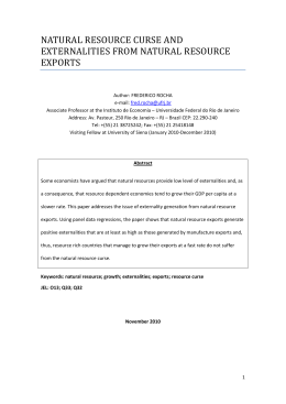
Figure 3.1: The quantity plotted is the energy (kinetic plus potential in each of the first four
√
modes). The time is given in thousands of computational cycles. Each cycle is 1/2 2
of the natural time unit. The initial form of the string was a single sine wave (mode
1). The energy of the higher modes never exceeded 6% of the total. (from [2]).
Fourier mode, λ = 1, in the notation of (). The objective of the experiment was to study
the energies stored in the first few Fourier modes, i.e. the quantities
Hλ ≡
where
r
Aλ =
´
1³ 2
Ȧλ + Ω2λ A2λ
2
µ
¶
N
2 X
iπλ
sin
Qi
N i=1
N
(3.22)
(3.23)
as a function of time, i.e. to test the onset of equipartition. Note that the decomposition
P of
the total energy in Fourier modes is not exact - but as long as α stays small, H ≈ λ Hλ
will hold.
Fig. 3.1 shows the time dependence of the energies of the first four modes. After an initial
redistribution, all of the energy (within 3%) returns to the lowest mode. The energy residing
in higher modes never exceeded 6 % of the total. Longer numerical studies have shown the
return of the energy to the initial mode to be a periodic phenomenon; the period is about
157 times the period of the lowest mode. The phenomenon is known as FPU recurrence.
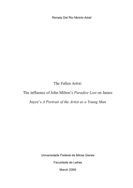
The results of a more recent numerical study on FPU recurrence[3] are summarized in
Fig. 3.2.
The Hamiltonian (3.21) is fairly generic. In fact, the original FPU paper describes a further study with quartic, rather than cubic, anharmonicities which exhibits similar behavior.
FPU recurrence has been shown to be a robust phenomenon. The upshot of those exhaustive
numerical observations is that anharmonic corrections to the Hamiltonian, contrary to the
original expectation which held them as agents that might help establish ergodicity, actually
appear to generate new forms of approximately periodic behavior. The process of under-
18
3 The FPU paradox
Figure 3.2: FPU recurrence time, divided by N 3 vs a scaling variable R = α(E/N )1/2 N 2 where
E/N ≈ [πB/(2N )]2 is the energy density. Typical values used by FPU correspond to
R À 1. The asymptotic regime is well described by the relationship Tr /N 3 = R−1/2
(from Ref. [3]).
standing the source of this behavior - also known as the FPU paradox - and relating it to
other manifestations of nonlinearity [4] has led to a profound change in theoretical physics.
19
4
The Korteweg - de Vries equation
4.1 Shallow water waves
Original context: Wave motion in shallow channels, cf. Scott-Russell1
Mathematical description due to Korteweg and deVries (KdV [6]). The equation arises in
wide variety of physical contexts (e.g. plasma physics, anharmonic lattice theory). Hence it
counts as one of the “canonical” soliton equations.
Long waves (typical length l) in a shallow channel l À h.
Small amplitude (¿ h) waves (weak nonlinearity)
Two-dimensional fluid flow (motion in lateral dimension of channel neglected)
x: horizontal direction, y: vertical direction
4.1.1 Background: hydrodynamics
Fluid velocity
~ ≡ ux̂ + v ŷ
V
(4.1)
Equations of (Eulerian) incompressible fluid dynamics
• continuity equation
• Euler equation
~ =0
∇·V
(4.2)
~
∂V
~ · ∇)V
~ = − 1 ∇p + ~g
+ (V
∂t
ρ
(4.3)
where ~g = −g ŷ plus
• irrotational flow (no vortices)
~ =0⇒V
~ = ∇Φ
∇×V
.
(4.4)
Using vector identity
~ · ∇)V
~ = 1 ∇V 2 − V
~ × (∇ × V
~)
(V
(4.5)
2
in (4.3) (only first term survives due to (4.4) ), and (4.4) in (4.2) transforms hydrodynamics
equations to
1 “I
was observing the motion of a boat which was rapidly drawn along a narrow channel by a pair of horses,
when the boat suddenly stopped - not so the mass of water in the channel which it had put in motion; it
accumulated round the prow of the vessel in a state of violent agitation, then suddenly leaving it behind,
rolled forward with great velocity, assuming the form of a large solitary elevation, a rounded, smooth
and well-defined heap of water, which continued its course along the channel apparently without change
of form or diminution of speed. I followed it on horseback, and overtook it still rolling on at a rate of
some eight or nine miles an hour, preserving its original figure some thirty feet long and a foot to a foot
and a half in height. Its height gradually diminished, and after a chase of one or two miles I lost it in
the windings of the channel. Such, in the month of August 1834, was my first chance interview with that
singular and beautiful phenomenon which I have called the Wave of translation.”[5]
20
4 The Korteweg - de Vries equation
1. continuity
4Φ = 0
2. Euler
,
(4.6)
p
∂Φ 1
+ (∇Φ)2 + + gy = 0
∂t
2
ρ
.
(4.7)
4.1.2 Statement of the problem; boundary conditions
The above eqs (4.6) and (4.7) must now be solved subject to the boundary conditions
1. bottom: no vertical motion of the fluid
v(x, y = 0) = 0
∀x
(4.8)
2. top: free surface defined as
y = h + η(x, t).
(4.9)
Velocity of free boundary coincides with fluid velocity,
dy
dt
=
v
=
∂η
∂η dx
+
∂t
∂x dt
∂η
∂η
+
u
∂t
∂x
hence
(4.10)
holds at the free surface.
The solution will involve two steps: first, find a general class of solutions of (4.6) which
satisfy the bottom BC (4.8), and then use this general class to determine the height profile
(4.9) by demanding that the Euler equation (4.7) be satisfied at the free surface, where p = 0
holds. The Euler equation can then be used to determine the pressure at any point.
4.1.3 Satisfying the bottom boundary condition
Consider the general form of an expansion (the height O(h) is small in a sense which will
be made precise below) of the type
The conditions
as
∂u
∂y
=
u =
v =
f (x) + f1 (x)y + f2 (x)y 2 + f3 (x)y 3 + · · ·
g1 (x)y + g2 (x)y 2 + g3 (x)y 3 + · · · .
∂v
∂x
∂u
∂x
and
(4.11)
∂v
= − ∂y
imposed by (4.6) can now be written, respectively,
f1 + 2f2 y + 3f3 y 2 = g1x y + g2x y 2
(4.12)
and
fx + f1 y + f2 y 2 = −g1 − 2g2 y − 3g3 y 2
(4.13)
from which
f1
2f2
3f3
= 0
(4.14)
=
=
(4.15)
(4.16)
21
g1x
g2x
4 The Korteweg - de Vries equation
and
fx
f1x
f2x
=
=
=
−g1
−2g2
−3g3
(4.17)
(4.18)
(4.19)
follow. Using the second set in the first, results in f1 = 0, 2f2 = −fxx , 2f3 = −1/2f1xx (= 0);
it follows that g2 = 0 and g3 = −1/3f2x = 1/3!fxxx . Collecting terms,
u
v
1
= f − fxx y 2 + O(y 4 )
2
1
= −fx y + fxxx y 3 .
3!
(4.20)
(4.21)
4.1.4 Euler equation at top boundary
Set p = 0 in (4.7) and differentiate with respect to x:
∂u 1 ∂ 2
∂η
+
(u + v 2 ) + g
=0
∂t
2 ∂x
∂t
.
(4.22)
The problem is now to solve the system of coupled differential equations (4.22) and (4.10)
using the expressions (4.20) and (4.21). Key: follow the scale of variation of the physical
quantities involved. First note that if the water height is not much different from h (small
nonlinearity), it will be useful to set
η = ²hη̄
(4.23)
Note ² is not a parameter of the problem. It simply serves as a “tag” to let us keep
track of scales. At the end we will have to check the consistency of the assumptions and
approximations made.
According to our assumption, the length scale on which the fluid profile varies along the x
direction is of the order l À h. In order to incorporate this assumption in the approximation,
I define a rescaled variable via
x = lx̄ .
(4.24)
√
Dimensional consideration determine a natural velocity scale c = gh. The motion should
be slow with respect to that scale - in agreement with small amplitude variations of the
profile. In other words, we expect u ¿ c. Note that from the leading orders of (4.20) and
(4.21)it follows that v is typically of order h/l ≡ δ smaller than u. It is therefore reasonable
to rescale
f
u
= ²cf¯
= ²cū
v
= δ²cv̄
(4.25)
(4.26)
.
(4.27)
Finally I use a rescaled time
t = t̄ l/c
.
(4.28)
2
With these rescalings, keeping lowest order terms, i.e. of O(²) and O(δ ), the rescaled
equations (4.20) and (4.21) become - on the surface ū =
v̄
=
1
f¯ − δ 2 f¯x̄x̄
2
1
−(1 + ²η̄)f¯x̄ + δ 2 f¯x̄x̄x̄
6
22
(4.29)
;
(4.30)
4 The Korteweg - de Vries equation
accordingly, the top boundary condition (4.10) and the Euler equation (4.22) transform to
1
f¯x̄ + η̄t̄ + ²(f¯η̄)x̄ − δ 2 f¯x̄x̄x̄
6
²
1
f¯t̄ + η̄x̄ + (f¯2 )x̄ − δ 2 f¯x̄x̄t̄
2
2
= 0
= 0
(4.31)
.
(4.32)
First we note that in the absence of nonlinearity (² = 0) and dispersion (δ = 0), free
wave propagation with unit velocity (in dimensionless units) occurs; in that (zeroth) order,
f¯ = η̄. But of course this is hypothetical because δ and ² are not parameters of the problem
- they just help us keep track of things! However, the zeroth order approximation is useful
in the sense that it suggests a coordinate transformation which absorbs the fastest time
dependence; let
ξ
τ
=
=
x̄ − t̄
²t̄ .
(4.33)
(4.34)
Keeping terms to first order in ² and δ 2 , we use the property
η̄x̄
η̄t̄
=
=
η̄ξ
−η̄ξ + η̄τ ²
(4.35)
(4.36)
(which holds for f¯ as well) transform the system (4.32) to
1
f¯ξ − η̄ξ + ²η̄τ + ²(η̄ 2 )ξ − δ 2 η̄ξξξ
6
1
² 2
¯
−fξ + η̄ξ + ²η̄τ + (η̄ )ξ + δ 2 η̄ξξξ
2
2
=
0
=
0
(4.37)
.
(4.38)
where we have used the property f¯ = η̄ in terms which contain ² or δ 2 factors. The sum of
(4.38) is
3
1
2²η̄τ + ²(η̄ 2 )ξ + δ 2 η̄ξξξ = 0 .
(4.39)
2
3
The three terms in (4.39) will be of the same order if δ 2 = O(²), i.e. if the nonlinearity
balances the dispersion. We choose ² = δ 2 /6. Note that the choice must be tested at the
end to check whether it satisfies the original requirements (small amplitude, long waves).
With this choice and the substitution η̄ = 4φ I arrive at the “canonical” KdV form,
φτ + 6φφξ + φξξξ = 0
.
(4.40)
4.1.5 A solitary wave
At this stage, without recourse to advanced mathematical techniques, it is possible to follow
the path of KdV and look for special, exact, propagating solutions of (4.40) of the type φ(s),
where s = ξ − λτ . (4.40) becomes
−λφs + 3(φ2 )s + φsss = 0
(4.41)
which has an obvious first integral
−λφ + 3φ2 + φss = const.
(4.42)
If we are looking for solutions which vanish at infinity (lims→∞ φ(s) = 0 and lims→∞ φs (s) =
0) the constant will be zero, i.e.
φss = λφ − 3φ2 =
23
d 1 2
( λφ − φ3 )
dφ 2
(4.43)
4 The Korteweg - de Vries equation
Multiplying both sides by 2φs we can integrate once more, obtaining
φ2s = λφ2 − 2φ3
(4.44)
where the integration constant must vanish once again (cf. above). Note that, if a solution
exists, the parameter λ must be > 0 and φ < λ/2. Taking the square root of (4.44) and
inverting the fractions I obtain
dφ
ds = ± √
(4.45)
φ λ − 2φ
which can be integrated directly, resulting in
φ(s) =
2 cosh2
λ
h√
λ
2 (s
i
− s0 )
(4.46)
where s0 is an arbitrary constant. (The plus sign in (4.45) has been chosen for s < s0 and
the minus for s > s0 ).
Note that the properties of the propagating solution (4.46) - except for its initial position,
which is determined by s0 - are all governed by a single parameter. If the velocity λ is
given, the amplitude is fixed at λ/2 and the spatial extent at 2λ−1/2 . In other words - in the
canonical units of (4.40) - a slow pulse will also have a small amplitude and a large spatial
extent.
4.1.6 Is the solitary wave a physical solution?
Eq. (4.46 ) is an exact, propagating, pulse-like solution of (4.40). But is it an acceptable
solution of the original problem? In other words, is the surface profile of low amplitude and is
it a long wave? To do this, we have to go back to the original variables, and convince ourselves
that (4.46) generates (some) acceptable solutions for the original problem (Exercise)
4.2 KdV as a limiting case of anharmonic lattice dynamics
Consider the 1-d anharmonic chain; atomic displacements are denoted by {un }; neighboring
atoms of mass m interact via anharmonic potentials of the type
V (r) =
1 2 1
kr + kbr3
2
3
(4.47)
where r is the distance between nearest neighbors. The equations of motion are
mq̈n
=
=
=
∂
[V (qn+1 − qn ) + V (qn − qn−1 ])
∂qn
k(qn+1 + qn−1 − 2qn ) − kb[−(qn+1 − qn )2 + (qn − qn−1 )2 ]
k(qn+1 + qn−1 − 2qn ) − kb(qn+1 + qn−1 − 2qn )(qn+1 − qn−1 ) .
−
(4.48)
If the displacements do not vary appreciably on the scale of the lattice constant a, we can
use a continuum approximation; keeping terms of fourth order in the lattice constant,
mq̈ ≡ qtt = ka2 qxx + ka4
2
qxxxx + kba2 qxx 2aqx
4!
,
where x = na is the continuum space variable; defining c2 = ka2 /m, this can be written as
1
1 2
qtt − qxx =
a qxxxx + 2αqx qxx
2
c
12
24
,
(4.49)
4 The Korteweg - de Vries equation
where α = ab provides a dimensionless measure of the anharmonicity.
I now look for solutions which vary smoothly in space, i.e. over a typical length of many
lattice spacings, and where the main time dependence is contained in the wave equation
part, i.e. of the form
x − ct
, δω0 t) ,
(4.50)
q(ξ, τ ) ≡ q(²
a
p
where ω0 = c/a = k/m, ² ¿ 1 and δ ¿ ²; the exact dependence of δ on ² will be fixed
later.
The relevant derivatives transform according to
qx
=
qxx
=
qxxx
=
qtt
=
²
qξ
a
³ ² ´2
qξξ
a
³ ² ´3
a¡
ω02
qξξξ
¢
² qξξ − 2²δqξτ + O(δ 2 )
2
.
Using them in (4.49) gives
2δqξτ +
1 3
² qξξξξ + 2αqξ qξξ = 0
12
which, after a rescaling
qξ (=
and setting
a
²
qx ) = − aφ
²
4α
,
(4.51)
(4.52)
2
δ=
1 3
²
24
can be reduced to the canonical KdV form
φτ − 6φφξ + φξξξ = 0
.
(4.53)
Note that the rescaling of length, i.e. the value of the small parameter ² is still a matter of
free choice, depending on the (initial) conditions of the problem.
The above analysis shows that one may legitimately suspect that nonlinear propagating
solitary waves will be generic in anharmonic lattices, at least for certain parameter ranges.
Again, one has to make sure that the solutions found from solving the KdV equation (4.53)
are appropriate for the original problem (4.49) (check consistency of approximations made).
4.3 KdV as a field theory
4.3.1 KdV Lagrangian
The KdV equation
ut − 3(u2x )x + uxxx = 0
(4.54)
can be derived from the Lagrangian
Z
L=
2 note
dxL(φ, φt , φx , φxx )
that this guarantees δ ¿ ² as demanded above.
25
(4.55)
4 The Korteweg - de Vries equation
where
L=
1
1
φx φt − φ3x − φ2xx
2
2
.
(4.56)
Note that because the Lagrangian density depends on the second derivative of the field,
(1.42) contain an extra term
µ
¶
d2
∂L
.
(4.57)
− 2
dx
∂φxx
Minimization of the action leads to the field equations of motion
φxt − 3(φ2x )x + φxxxx = 0
(4.58)
which reduces to (4.54) upon the substitution
φx = u .
(4.59)
Continuous symmetries of the Lagrangian will again give rise to an equation like (1.44), with
an extra term
∂L
δφxx
(4.60)
∂φxx
on the left-hand side. The above modifications generate an extra contribution
∂L
d2
δφxx − 2
∂φxx
dx
µ
∂L
∂φxx
¶
δφ
(4.61)
to the left-hand side of (1.45).
4.3.2 Symmetries and conserved quantities
For some infinitesimal transformations (cf. section ) one can verify explicitly that δφxx =
d2 δφ/dx2 . If this is the case, the integral over all space of the extra contribution (4.61) can
easily be seen to vanish (repeated integration by parts of either of the two terms). In this
case, the standard symmetries are reflected in the same standard conservation (with the
same densities of conserved quantities), as in section .... .
Translational invariance in space
Conservation of the total momentum
Z
Z
Z ∞
1 ∞
1 ∞
∂L
φx = −
dx φ2x = −
dx u2
P =−
dx
∂φ
2
2
t
−∞
−∞
−∞
.
(4.62)
Translational invariance in time
Conservation of the total energy
µ
¶
Z ∞
∂L
H=
dx
φt − L
∂φt
−∞
¶
1 2
3
= −
dx
φ + φx
2 xx
−∞
¶
µ
Z ∞
1 2
3
u +u
.
= −
dx
2 x
−∞
Z
26
∞
µ
(4.63)
4 The Korteweg - de Vries equation
Conservation of mass
The symmetry φ → φ + ² generates δφ = ², and all other variations are zero. From (1.45),
conservation of
Z ∞
Z
Z
∂L
1 ∞
1 ∞
dx
=
dx φx =
dx u ,
(4.64)
M=
∂φt
2 −∞
2 −∞
−∞
the total “mass”, is deduced.
Galilei invariance
The transformation x → x − ²t, φ(x, t) → φ(x − ²t) − ²x (or in terms of the u-field, u(x, t) →
u − ², generates (cf. section ....)
x → x − ²t
δφ = φ(x − ²t) − φ(x) − ²x = −²tφx − ²x
δφt = φt (x − ²t) − φt (x) = −²tφxt
δφx = φx (x − ²t) − φx (x) − ² = −²tφxx − ²
dL
dL
δL =
δx = − ²t ⇒ J1 = −tL , J0 = 0
dx
dx
.
(4.65)
Owing to δφxx = (δφ)xx there are no extra terms in the conserved currents. Eq. (1.45)
applies. Since δφx = (δφ)x the two last terms in the left-hand side of (1.45) combine to
form a total space derivative; similarly, because of δφt = (δφ)t , the first two terms combine
to form a total time derivative, i.e. the conserved density is
∂L
1
δφ/² = φx (−tφx − x) ,
∂φt
2
or, integrating over all space, and dividing by the total mass M ,
Z ∞
1
P
u
X̄ =
t + const.
dx x =
M −∞
2
M
which expresses the fact that the center of mass moves at a constant velocity.
4.3.3 KdV as a Hamiltonian field theory
27
(4.66)
(4.67)
5
Solving KdV by inverse scattering
5.1 Isospectral property
Given the KdV equation
ut − 6uux + uxxx = 0
(5.1)
and a well behaved initial condition u(x, 0), which vanishes at infinity, it is possible to
determine the time evolution u(x, t) in terms of a general scheme, which is known as inverse
scattering theory.
The scheme is based on the following particular property of (5.1):
Given the linear operator
2
L(t) = −∂xx
+ u(x, t)
(5.2)
whose parametric time dependence is governed by (5.1), and the associated eigenvalue equation
L(t)ψj (x, t) = λj (t)ψj (x, t) ,
(5.3)
it can be shown that
dλj
=0
dt
.
(5.4)
5.2 Lax pairs
The “isospectral” property can be formulated somewhat more generally: Suppose we can
construct a linear, self-adjoint operator B = B † , dependent on u and such that
iLt ≡ i
dL
L(t + ∆) − L(t)
≡ i lim
= [L, B]
∆→0
dt
∆
(5.5)
holds as an operator identity, i.e.
iLt f = [L, B]f
∀f
⇔ (5.1) .
(5.6)
The operators L and B are then called a Lax pair. The time evolution of L is governed by
L(t) = U (t)L(0)U †
(5.7)
where
U = eiBt
.
(5.8)
Consider (5.3) at t = 0, and apply the operator U (t) to both sides from the left, i.e.
U (t)L(0)
U † (t)U (t)ψj (0) = λj (0)U (t)ψj (0)
(5.9)
where, in addition I have inserted a factor U † U = 1. It can be recognized immediately that
the l.h.s. of (5.9) and (5.3) are identical, provided
ψj (t) = U (t)ψj (0)
28
,
(5.10)
5 Solving KdV by inverse scattering
and that, in order for the r.h.sides to coincide, I must have
λ(t) = λ(0)
∀t
(5.11)
(isospectral property).
The form of the operator B in the KdV case is
3
B = 4i∂xxx
− 3i (u∂x + ∂x u)
(5.12)
(verify explicitly (5.6).
5.3 Inverse scattering transform: the idea
The isospectral property tentatively suggests that it might possible to proceed as follows:
• solve the linear problem (5.3) at time t = 0, i.e. determine the eigenvalues {λj } and
the eigenfunctions {ψj (x, 0)} from the known u(x, 0).
• determine the evolution of the eigenfunctions from (5.10) at a later time t.
• try to solve the “inverse problem” of determining the “potential” u(x, t) from the
known spectra and eigenfunctions at the time t.
In fact, the last step is the well known problem of inverse scattering theory in quantum
mechanics, where physicists had tried to extract information on the nature of interparticle
interactions from analyzing particle scattering data. The one-dimensional problem (corresponding to a spherically symmetric potentials in 3 dimensions) was completely solved in
the 1950’s (Gel’fand, Levitan & Marchenko). I will present the solution below, but before
doing that, let me outline some broad features:
“Scattering data”in the mathematical sense are the asymptotic properties of the solution
of the associated linear problem, i.e. the properties far from the source of scattering, where
the potential is effectively zero. What GLM have shown is that you can reconstruct the
potential from the scattering data. Furthermore, it turns out that the operator B takes
an especially simple form in the asymptotic limit, which allows us to write down an exact,
analytic formula for the time evolution of scattering data. Evolution of the scattering data
is the easy part of the game. But then if I only need scattering data at time t, and I know
how these data evolve in time, all the input I need is the scattering data for the potential
u(x, 0). This is exactly the program of the inverse scattering transform (IST). Because it is
based only on the asymptotic part of the solution of the associated linear problem, it can
be written down in closed form. I summarize the IST program schematically:
1. determine the scattering data S of the linear problem (5.3) at time t = 0, from the
known u(x, 0).
2. determine the evolution of the scattering data S(t) at a later time t from the asymptotic
from of the operator B.
3. do the inverse problem at time t, i.e. determine the potential u(x, t) from the known
scattering data S(t).
5.4 The inverse scattering transform
5.4.1 The direct problem
This is just a summary of properties known from elementary quantum mechanics.
29
5 Solving KdV by inverse scattering
Jost solutions
The linear eigenvalue problem
·
−
¸
∂
+
u(x)
ψ(x) = k 2 ψ(x)
∂x2
(5.13)
has, in general, a discrete and a continuum spectrum, corresponding to imaginary and real
values of k respectively. For real k there are in general two linearly independent solutions.
Such a linearly independent set is provided by the Jost solutions:
f1 (x, k) ∼
f2 (x, k) ∼
eikx x → ∞
e−ikx x → −∞
.
The Jost solutions of (5.13) satisfy the integral equations
Z ∞
ikx
f1 (x, k) = e −
dx0 G(x, x0 )f1 (x0 , k)
x
Z x
−ikx
f2 (x, k) = e
+
dx0 G(x, x0 )f2 (x0 , k)
(5.14)
(5.15)
−∞
where
sin k(x − x0 )
u(x0 ) .
(5.16)
k
Eqs. (5.15) can be analytically continued to the upper half plane of complex k. Some
information on the analytic properties can be obtained by considering the lowest iteration,
0
where we substitute f1 (x0 , k) = eikx in the r.h.s. of the first equation. This gives
G(x, x0 ) =
Z
f1 (x, k)
∞
0
0
0
eik(x −x) − e−ik(x −x)
u(x0 )eikx
2ik
x
Z ∞
0
ikx
ikx 1
≈ e −e
dx0 {1 − e2ik(x −x) }u(x0 )
2ik x
≈ eikx −
dx0
(5.17)
which can be thought of as the beginning of a systematic expansion in inverse powers of k.
Note that since x0 − x > 0, the exponential will be convergent in the upper-half plane of k;
therefore, if the potential vanishes sufficiently rapidly at infinity, I estimate
g1 (x, k) ≡ f1 (x, k) − eikx ∼ eikx h(x, k)
(5.18)
where h vanishes as 1/k for high values of k.
The property
f2 (x, k) = a(k)f1 (−k, x) + b(k)f1 (k, x) .
(5.19)
will be useful.
For bound states, corresponding to k = iκ, the Jost solutions are degenerate.
Asymptotic scattering data
The asymptotic (scattering) data of (5.3) is defined as follows:
• discrete spectrum (bound states)
λn = −κ2n
n = 1, · · · , N
30
,
(5.20)
5 Solving KdV by inverse scattering
where κn > 0;
ψn (x) =
=
f1 (x, k) ∼ e−κn x x → ∞
Cn f2 (x, k) ∼ Cn eκn x x → −∞
.
(5.21)
I will also need the normalization integral of each bound state
Z ∞
Z ∞
1
2
=
dxψn (x) =
dxf12 (x, iκn )
αn
−∞
−∞
(5.22)
• continuous spectrum (scattering states)
λ(k) = k 2
−∞<k <∞
.
(5.23)
The “physical ”scattering states corresponding to waves incident from the right, are
ψ(x, k) ∼
∼
e−ikx + R(k)eikx x → ∞
T (k)e−ikx x → −∞ .
(5.24)
where R(k), T (k) are, respectively, the reflection and transmission coefficients, which
satisfy
|R(k)|2 + |T (k)|2 = 1 .
The Jost solutions are related to the physical solution (5.24) via
ψ(x, k) = T (k)f2 (x, k) = f1 (x, −k) + R(k)f1 (x, k)
∀x.
(5.25)
This identifies a(k) = 1/T (k) and b(k) = R(k)/T (k).
The complete set of scattering data for any one dimensional potential of a Schroedinger-type
equation is
S ≡ [{κn , Cn , αn }, n = 1 · · · , N ; T (k), R(k)].
(5.26)
In fact, for the purposes of performing the inverse scattering transform I will only need the
reduced set 1
S ≡ [{κn , αn }, n = 1 · · · , N ; R(k)]
(5.27)
5.4.2 Time evolution of scattering data
I promised this will be the easy part. The operator B has the property
lim
|x|→±∞
3
= B ∗ = 4i∂xxx
.
(5.28)
Since
∂
ψj (x, t) = iBψj (x, t)
(5.29)
∂t
holds for all eigenfunctions, we can apply in the asymptotic regime, where B ∼ B ∗ .
• In the case of a discrete eigenfunction, this gives
ψn (x) ∼
∼
3
e−κn x+4κn t
Cn e
κn x−4κ3n t
1 Note
x→∞
x → −∞
,
(5.30)
that if scattering theory is to make sense, the potential must be vanishing at (±)infinity. I have not
specified the minimal exact mathematical conditions which satisfy this demand.
31
5 Solving KdV by inverse scattering
or, in keeping with the agreed normalization of the type (5.21), I multiply with a factor
3
e−4κn t , and obtain
e−κn x x → ∞
Cn (t)eκn x x → −∞
ψn (x) ∼
∼
with
3
Cn (t) = Cn (0)e−8κn t
,
(5.31)
.
(5.32)
• In the case of Jost solutions I obtain
f1 (k, x)
f2 (k, x)
∼ eikx+4ik
∼ e
3
t
x→∞
−ikx−4ik3 t
x → −∞
;
(5.33)
the physical solution therefore evolves according to
ψ(k, x)
3
∼ e−ikx−4ik t + R(k)eikx+4ik
∼ T (k)e−ikx−4ik
or, multiplying both by a factor e
4ik3 t
ψ(k, x) ∼
∼
where
3
t
3
x → −∞
t
x→∞
,
, to keep the standard normalization of ()
e−ikx + R(k, t)eikx x → ∞
T (k)e−ikx x → −∞ ,
R(k, t) = R(k)e8ik
3
t
.
(5.34)
The scattering data evolve according to (5.32) and (5.34). The transmission coefficient T (k)
stays constant in time.
5.4.3 Reconstructing the potential from scattering data (inverse
scattering problem)
Reconstruction of the potential from scattering data is an old problem in quantum mechanics. A complete solution has been given in one dimension, subject to fairly general
conditions, by Gelfand and Levitan [7] and Marchenko[8]. Reviews by Faddeyev[9] and
Scott[10]. Definition of the problem: Given the eigenvalue equation
·
¸
d2
− 2 + u(x) ψ(x) = k 2 ψ(x)
(5.35)
dx
determine u(x) from scattering data in the form of eqs. (5.27).
Fourier transforms of the g(x, k) functions
Z ∞
1
ĝj (x, y) =
dk e−iky gj (x, k) ,
2π −∞
where j = 1, 2, with an inverse
Z ∞
gj (x, k) =
dy eiky ĝj (x, y) .
(5.36)
(5.37)
−∞
Note that, due to the analytic properties of f1 (cf. (5.18), which allows to close the contour
of (5.36) from above without finding any singularities)
ĝ1 (x, y) = 0
if
y<x
.
(5.38)
ĝ2 (x, y) = 0
if
y>x
.
(5.39)
Similarly,
32
5 Solving KdV by inverse scattering
Relating ĝ1 (x, x) to the potential u(x)
The starting point is to recognize that
¶
µ 2
¶
µ 2
∂
∂
2
2
+ k − u g1 (x, k) =
+ k − u (f1 (x, k) − 1) = u(x)eikx
∂x2
∂x2
;
multiplying both sides by e−iky /2π and integrating over all k, I obtain
µ 2
¶
∂
∂2
− 2 − u(x) ĝ1 (x, y) = u(x) δ(x − y) ;
∂x2
∂y
(5.40)
(5.41)
defining new variables ζ = (x + y)/2, η = y − x, I use ∂x2 − ∂y2 = 2∂η ∂ζ , to transform (5.41)
to
³
³
∂2
η´
η´
η
η´ ³
η
−2
ĝ1 ζ − , ζ +
−u ζ −
ĝ1 ζ − , ζ +
∂η∂ζ
2
2
2
2
2
η
= u(ζ − )δ(−η) ,
2
which can be integrated over an interval of length ² around η = 0. The result is
−2
∂
ĝ1 (ζ, ζ) − ²u(ζ)ĝ1 (ζ, ζ) = −u(ζ) ,
∂ζ
(5.42)
which in the limit ² → 0 becomes
u(x) = −2
d
ĝ1 (x, x)
dx
(5.43)
where I have reverted to the original variables.
Relating g1 (x, y) to the scattering data
Define Fourier transforms
Z
T̂ (y)
∞
=
−∞
Z ∞
R̂(y)
=
−∞
dk −iky
e
[T (k) − 1]
2π
dk iky
e R(k) .
2π
(5.44)
(5.45)
Rewrite (5.25) as
£
¤
T (k)f2 (x, k) = f1 (x, −k) + R(k) f1 (x, k) − eikx + eikx
;
(5.46)
adding −f2 (x, k) to both sides and adding and subtracting e−ikx to the right hand side gives
(T (k) − 1) f2 (x, k) = g1 (x, −k) − g2 (x, k) + R(k)g1 (x, k) + R(k)eikx
multiplying both sides by eiky /2π and integrating over all k produces
Z ∞
dk iky
e [T (k) − 1] f2 (x, k) = ĝ1 (x, y) − ĝ2 (x, y) +
2π
−∞
Z ∞
dy 0 R̂(y + y 0 ) ĝ1 (x, y 0 ) + R̂(x + y)
−∞
Lemma: T (k) has only simple poles
33
;
(5.47)
(5.48)
5 Solving KdV by inverse scattering
It can be shown that the transmission coefficient T (k) is analytic in the upper half plane,
including the real axis, except for simple poles which correspond to the bound states, i.e. at
k = iκn . In the neighborhood of such a pole
T (k) ≈ i
Cn αn
k − iκn
,
(5.49)
where
Z ∞
1
=
dx[f1 (x, iκn )]2
αn
−∞
is the normalization integral of the bound state.
(5.50)
Using the above lemma, it is possible to compute the integral in the left-hand side of
(5.48) by closing the contour from above. The contribution from each bound state is
2πie−κn y i
1
Cn αn f2 (x, iκn )
2π
= −αn e−κn y f1 (x, iκn )
= −αn e−κn y g1 (x, iκn ) − αn e−κn (x+y)
where I have used the fact that Jost states are degenerate if k = κn (cf. Eq. (5.21)).
Moreover, I only need (5.48) for x ≤ y, since otherwise ĝ1 (x, y) = 0. Defining a combined
kernel which incorporates all scattering data,
K̂(z) = R̂(z) +
N
X
αn e−κn z
,
(5.51)
n=1
I finally obtain
Z
∞
ĝ1 (x, y) + K̂(x + y) +
dy 0 K̂(y + y 0 ) ĝ1 (x, y 0 )
=
0
if x ≤ y
(5.52)
ĝ1 (x, y)
=
0
if x > y
(5.53)
−∞
(Gel’fand, Levitan, Marchenko equation).
5.4.4 IST summary
In order to solve the initial value problem of the KdV equation (5.1) we proceed as follows:
• Extract initial scattering data for the associated linear problem (5.13),
{κn , αn ; n = 1 · · · , N }, {R(k), −∞ < k < ∞}
(5.54)
from potential u(x) at time 0.
• Define the scattering kernel at time t:
Z ∞
N
X
3
dk ikz+8ik3 t
K̂(z; t) =
e
R(k) +
αn e−κn z+8κn t
2π
−∞
n=1
• Solve the Gel’fand, Levitan, Marchenko equation for x ≤ y,
Z ∞
ĝ1 (x, y; t) + K̂(x + y; t) +
dy 0 K̂(y + y 0 ; t) ĝ1 (x, y 0 ; t) = 0
.
(5.55)
.
(5.56)
x
• Extract the limit
d
ĝ1 (x, x+ ; t) .
(5.57)
dx
Note that (i) I have explicitly included the parametric dependence on time, and (ii)
the normalization integral αn has a time dependence such that the product Cn αn stays
constant (cf. time-independence of the transmission coefficient).
u(x, t) = −2
34
5 Solving KdV by inverse scattering
5.5 Application of the IST: reflectionless potentials
Suppose the scattering kernel (5.51) contains only bound states, i.e. R(k) = 0. This would
correspond to a reflectionless potential in the original quantum mechanical context. In this
case it turns out that I can systematically derive a whole class of solutions to the original
KdV equation by just solving the GLM equation (5.56) and taking the appropriate limit
(5.57).
5.5.1 A single bound state
The scattering kernel has the form
K̂(z; t) = αe−κz+8κ
3
t
.
(5.58)
I will look for solutions of (5.56) which are separable, i.e.
ĝ1 (x, y; t) = e−κy h(x, t) ;
with the above Ansatz, (5.56) tranforms to
·
Z
8κ3 t
−κx
h(x, t) + αe
e
+ h(x, t)
(5.59)
¸
∞
0 −2ky 0
dy e
=0
;
x
inserting the expression for the integral, (2κ)−1 e−2κx , and setting α = 2κe2δ , I obtain
h
i
3
3
h(x, t) 1 + e2δ e−2κx+8κ t = −αe−κx+8κ t
3
ĝ1 (x, y; t) = −2κ
e−κ(x+y)+8κ t+2δ
1 + e−[2κx−8κ3 t−2δ]
;
the limiting form for y = x is
ĝ1 (x, x; t) = −2κ
it follows that
u(x; t) = −2
1
1+
e2[κx−4κ3 t−δ]
;
d
2κ2
ĝ1 (x, x; t) = −
dx
cosh2 [κ(x − 4κ2 t) − δ]
(5.60)
which is identical to the solitary wave (4.46), if we identify λ in (4.46) with 4κ2 in (5.60).
Comments:
• the velocity of the wave corresponds (to within a factor of -4) to the eigenvalue of the
associated problem.
• The velocity coincides with the ratio P/M (cf. symmetries conservation laws; show
this (exercise)).
• Note that I made no attempt to guess the form of the wave. The form was “imposed” by
the separation ansatz (5.59), i.e. it is “built-in” in the association of the KdV equation
with the linear eigenvalue problem. This will be useful in the next subsection, where
I will try to construct solutions that correspond to multiple bound states.
• It is of course possible to treat the “proper” initial value problem. Starting with any
localized potential which may support a bound state, one can perform the IST steps.
Exercise: do this (i) for an attractive delta function potential −µδ(x), and (ii) for a
potential of the type −N (N + 1)sech2 x, where N is an integer; (hint: in case (ii) the
form of the solution is an example of the case discussed in the next subsection).
35
5 Solving KdV by inverse scattering
5.5.2 Multiple bound states
Again, I will restrict myself to the case where the reflection coefficient vanishes. The scattering kernel has the form
N
X
αi (t) e−κi z .
(5.61)
K̂(z; t) =
i=1
where αi (t) = αi e
ansatz (5.59)
8κ3i t
carries the time dependence. A generalized form of the separation
ĝ1 (x, y; t) =
N
X
e−κi y hi (x, t)
(5.62)
i=1
transforms the GLM equation (5.56) to
N
X
e−κi y { hi (x, t) + αi (t)e−κi x +
i=1
N
X
αi (t) −(κi +κj )x
e
hj (x, t)} = 0
κ + κj
j=1 i
,
which must hold for all y > x; hence, in nonsymmetric matrix form,
N
X
Aij hj (x, t) = Ci (x, t)
(5.63)
j=1
where
Aij (x, t) = δij +
αi (t) −(κi +κj )x
e
κi + κj
(5.64)
and
Cj (x, t) = −αi (t)e−κi x
Thus




1
hj =
det 

det A


A11
A21
·
A12
A22
·
···
···
···
C1
C2
C3
·
·
·
.
(5.65)
A1 j+1
A2 j+1
·
···
···
···




.



where the jth column in the matrix A has been substituted by the vector

A11 A12 · · · C1 e−κj x A1 j+1 · · ·
 A21 A22 · · · C2 e−κj x A2 j+1 · · ·

N
 ·
1 X
·
· · · C3 e−κj x
·
···
ĝ1 (x, x) =
det 

·
det A j=1


·
·
(5.66)
C; it follows that




;



(5.67)
note however that, since
dAij
= −αi e−(κi +κj )x = Ci e−κj x
dx
,
this is equivalent to
ĝ1 (x, x) =
d
ln det A .
dx
36
(5.68)
5 Solving KdV by inverse scattering
At this stage it is convenient to introduce the symmetrized form of the matrix A, obtained
by  = DAD−1 , where Dij = (αi )−1/2 δij , i.e.
Âij (x, t) = δij +
(αi αj )1/2 −(κi +κj )x
e
κi + κj
,
(5.69)
whereupon
d2
ln det Â
(5.70)
dx2
where I have reintroduced the time dependence, with the understanding that it arises solely
from the αi s.
u(x, t) = −2
Application: N = 2, the two-soliton solution
In the case N = 2
det  = 1 +
or, setting
α1 −2κ1 x
α1 −2κ2 x
α1 α2
e
+
e
+
2κ1
2κ1
4κ1 κ2
κ1 − κ2
≡ e−∆
κ1 + κ2
,
µ
κ1 − κ2
κ1 + κ2
αj ≡ 2κj e2θj +∆
∆
¶2
e−2(κ1 +κ2 )x
,
∆
det  = 1 + e−2(κ1 x−θ1 − 2 ) + e−2(κ2 x−θ2 − 2 ) + e−2[(κ1 +κ2 )x−(θ1 +θ2 )]
(5.71)
.
(5.72)
Note that now the time dependence is carried by the θj ’s, i.e.,
θj → θj (t) = θj0 + 4κ3j t
(5.73)
In order to extract the asymptotic behavior of u(x, t) at early and late times, I proceed as
follows: Assume κ1 > κ2 without loss of generality. Then as, t → −∞, at sufficiently early
times, it is possible to satisfy the double inequality
θ1
θ2
¿
κ1
κ2
It is easy to see that, unless x ≈ κθ11 or x ≈
will be vanishingly small. This is true
• for x À
θ2
κ2 ,
θ2
κ2 ,
.
the 2nd derivative of the expression (5.72)
because the last three terms vanish, leaving det  = 1
• for x ¿ κθ11 , because, although the three last terms are all exponentially large, the last
one will be dominant. This leaves ln det  ∝ x and the second derivative vanishes.
• for κθ11 ¿ x ¿ κθ22 the second term will be exponentially small, and the third term be
much larger than the last. Again, ln det  ∝ x and the second derivative vanishes.
This leaves the cases where x is appreciably near either κθ11 or κθ22 . In the first case, the
contributions to (5.72) come from the 3rd and 4th terms, i.e.
h
i
∆
∆
,
det  ≈ e−2(κ2 x−θ2 − 2 ) 1 + e−2(κ1 x−θ1 + 2 )
or,
ln det  ≈ −2(κ2 x − θ2 −
·
¸
∆
∆
∆
) − (κ1 x − θ1 + ) + ln 2 cosh(κ1 x − θ1 + )
2
2
2
37
,
5 Solving KdV by inverse scattering
κ1=2
κ2=1
θ1 /κ1= -2.
0
θ2 /κ2= -1.
0
0.4
8.000
7.000
6.000
0.2
5.000
t
0.5
4.000
0.0
3.000
t
5
1.950
0
0.0
1.000
-0.2
x
0
-5
-5
0
5
x
Figure 5.1: The two-soliton solution [−u(x, t)] of the KdV equation as a function of space and time.
Left panel: a 3-d plot shows the collision of the two solitons. Right panel: a contour
plot of the same function; note the asymptotic motion of the local maxima and the
phase shifts as a result of the interaction.
and hence
u(x, t) ≈ −2κ21 sech2 (κ1 x − θ1 +
∆
)
2
if
x ≈ θ1 /κ1
Similarly, it can be shown that
u(x, t) ≈ −2κ22 sech2 (κ2 x − θ2 −
∆
) if
2
x ≈ θ2 /κ2
.
Combining the above, and reintroducing the explicit time dependence, I can write that
u(x, t) ∼ −2
2
X
κ2j sech2 (κj x − 4κ3j t − θj0 ±
j=1
∆
) if
2
t → −∞
,
(5.74)
where the upper sign holds for j = 1, and the lower for j = 2. The above analysis can be
repeated almost verbatim for asymptotically late times and leads to
u(x, t) ∼ −2
2
X
κ2j sech2 (κj x − 4κ3j t − θj0 ∓
j=1
∆
)
2
if
t→∞
.
(5.75)
The above equations describe the soliton property in a mathematically exact fashion. As we
follow the evolution from very early to very late times, we see the larger - and faster - local
compression reach the smaller - and slower - , interact with it in an apparently intricate
fashion, and then disengage itself and resume its motion with the same velocity. Both waves
maintain shape, amplitude and speed. The interaction does however leave a signature. The
center of mass of each wave becomes slightly displaced; the fastest by an amount of ∆/κ1
38
5 Solving KdV by inverse scattering
(forwards), the slower by an amount of −∆/κ2 (backwards). Note that because the mass
of each soliton is proportional to κj , the center of mass of the combined two-soliton system
moves at a constant speed before and after the two-soliton collision. This type of elastic,
transparent interaction which leaves velocities unchanged and results only in spatial shifts2
is characteristic of soliton bearing systems, and accounts for their remarkable dynamical
properties.
The analysis can be generalized to the N −soliton solution. It can be shown that phase
shifts are pairwise additive, i.e. the total phase shift of any soliton as a result of its interaction
with the other N − 1 solitons is the sum of the N − 1 phase shifts resulting from the N − 1
collisions.
Fig. 5.1 exhibits graphically the dependence of the two-soliton solution on space and time.
5.6 Integrals of motion
It is possible to deal with integrals of motion in a systematic fashion, by following the
analytic structure of the scattering data. Recall that the transmission coefficient does not
carry any time dependence under the IST, i.e. it can be treated as a constant of the motion!
5.6.1 Lemma: a useful representation of a(k)
Given the fact that a(k) (recall that a is the inverse of the transmission coefficient) has
simple zeros in the upper half of the complex plane, the following identity holds:
!
Ã
Z ∞
N
0 2
X
1
k − kj
0 ln |a(k )|
ln a(k) =
(5.76)
dk
+
ln
2πi −∞
k0 − k
k − kj∗
j=1
(cf. appendix ...).
5.6.2 Asymptotic expansions of a(k)
The asymptotic expansion
ln a(k) ∼
∞
X
Jn
n
(2ik)
n=1
(5.77)
holds for |k| > max{|kj |}.
Multiply both sides of (5.77) by k l−1 /(2πi) and integrate over a circle of radius R >
max{|kj |} centered at the origin of the complex k-plane. The only term which survives in
the sum is that with j = l, hence
I
1
−l
dk k l−1 ln a(k) ;
(2i) Jl =
2πi
performing the dk integration in the first term of (5.76) generates a contribution −k 0 l−1 .
The second term can be integrated by parts and generates contributions from all poles. This
results in
Z ∞
N
X
¢
1
1 ¡ ∗l
Jl
l−1
2
=
−
dk
k
ln
|a(k)|
+
kj − kjl
.
(5.78)
(2i)l
2πi −∞
l
j=1
2 the
term “phase shifts” is generically applicable.
39
5 Solving KdV by inverse scattering
So far this has been general. Applying to the KdV equation, I set kj = iκj ; note that the
terms in the discrete sum vanish if l is even. Due to the reflection symmetry |a(k)| = |a(−k)|,
the integrals vanish as well for even l. This leaves
J2m+1
= −(−1)m
22m+1
Z
∞
dk k 2m ln |a(k)|2 + 2
−∞
N
X
κ2m+1
j
2m
+1
j=1
.
(5.79)
In what follows, I will relate the Jl s - which are by definition constants of the motion, since
they only depend on a(k) and bound state eigenvalues - to the family of conserved quantities
generated in the previous section, independently of the IST.
From the general property of the Jost functions
I deduce that if Imk > 0
f2 (x, k) = a(k)f1 (x, −k) + b(k)f1 (x, k)
(5.80)
¤
£
lim f2 (x, k)eikx = a(k) .
(5.81)
x→∞
This is because in the limit of large positive x the first term in (5.80), f1 (x, −k) ∼ e−ikx is
exponentially large and the second f1 (x, −k) ∼ e−ikx is exponentially small. On the other
hand,
£
¤
lim f2 (x, k)eikx = 1 .
(5.82)
x→−∞
holds by definition. Knowledge of the two limits allows me to define
σ(x) =
with the property
ª¤ f 0
d £ ©
ln f2 (x, k)eikx = 2 + ik
dx
f2
Z
(5.83)
∞
dx σ(x) = ln a(k)
.
(5.84)
−∞
Now we can use the fact that f2 is a solution of the associated linear problem, to derive
a differential equation for σ in terms of u. To do this I multiply both sides of (5.83) and
differentiate with respect to x. This gives
f200 + ikf20 = f20 σ + f2 σ 0
,
or
uf2 − k 2 f2 + ikf20 = f20 σ + f2 σ 0
;
substituting f20 = (σ − ik)f2 generates
σ 0 − 2ikσ + σ 2 − u = 0
(5.85)
a nonlinear ordinary first order differential equation of the Ricatti type.
I can now try to generate an asymptotic solution of the Ricatti equation (5.85),
σ(x, k) ∼
∞
X
σn (x, k)
(2ik)n
n=1
where I note that, because of (5.77) and (5.84),
Z ∞
dx σn (x) = Jn
−∞
40
.
(5.86)
(5.87)
5 Solving KdV by inverse scattering
Indeed, I note that the asymptotic ansatz (5.86) in (5.85) generates the recurrence relationships
n−1
X
d
σn+1 (x) =
σn (x) +
σj (x)σn−j (x) , n = 2, 3, · · ·
(5.88)
dx
j=1
with σ1 (x) = −u(x). This generates a countable infinity of conserved densities. The first
few are
σ2
σ3
σ4
σ5
=
=
=
=
ux
−uxx + u2
−uxxx + 2(u2 )x
−uxxxx + (u2 )xx + u2x + 2uuxx − 2u3
.
(5.89)
(5.90)
(5.91)
(5.92)
Note that the even σn ’s are total derivatives, i.e. they generate trivial, vanishing integrals;
we know this, since the corresponding Jn ’s vanish. The first few odd σn ’s generate the mass,
momentum, and energy integrals of section ....
5.6.3 IST as a canonical transformation to action-angle variables
It can be shown [] that the inverse scattering transform is a canonical transformation from
the original field variables to action-angle variables. The scattering data of the IST are
in essence action-angle variables. This demonstrates the KdV Hamiltonian system is completely integrable.
41
6
Solitons in anharmonic lattice
dynamics: the Toda lattice
The Toda lattice [11] is a unique example of a nonlinear discrete particle system which is
completely integrable. Although the property of complete integrability is certainly a singular
feature due to the peculiarity of the lattice potential, the model has been extremely useful
as a theoretical laboratory for the exploration of a number of novel concepts and phenomena
related to loss-free supersonic pulse propagation.
6.1 The model
The Hamiltonian
H=
X ½ p2
n
2m
n
where
φ(r) =
¾
+ φ(qn − qn−1 )
ª
a © −br
e
+ br − 1
b
(6.1)
(6.2)
describes a chain of N particles with equal mass m, which interact via nearest-neighbor
repulsive potential of exponential form. The range of the potential is given by 1/b and
its strength by a/b. The linear term in the potential represents an external force which is
necessary to achieve confinement. Important limiting cases of (6.2) are:
• the harmonic limit
a → ∞, b → 0, ab → k
which leads to
φ(r) =
1 2
kr
2
;
• the hard-sphere limit
b→∞
(i.e. the range approaches zero) with a finite, which leads to
φ(r)
=
0
=
∞
if r > 0
if r < 0
.
I will, from now on, set a = 1, b = 1, m = 1. Units will be reintroduced when appropriate.
The equations of motion are
q̇n
=
pn
ṗn
=
e−(qn −qn−1 ) − e−(qn+1 −qn )
42
(6.3)
6 Solitons in anharmonic lattice dynamics: the Toda lattice
6.2 The dual lattice
Consider the variables
rn = qn − qn−1
which describe the difference in displacements of neighboring sites. Differentiating both
sides with respect to time gives
ṙ1
ṙ2
ṙj
= q̇1 − q̇0
= q̇2 − q̇1
= q̇j − q̇j−1
.
Summing left and right sides separately gives allows me to express the velocity coordinates
as
j
X
q̇j =
ṙl ,
(6.4)
l=1
where I have assumed q̇0 = 0. The total kinetic energy is
à n !2
N
1X X
ṙl
T =
2 n=1
.
l=1
If I now define new momentum variables, conjugate to the rn coordinates, via
sj =
∂T
∂ ṙj
= ṙ1 + · · · + ṙj
+ ṙ1 + · · · + ṙj+1
+ ···
+ ṙ1 + · · · + ṙN ,
the sj ’s will satisfy
sj − sj+1 = ṙ1 + · · · ṙj = q̇j
(6.5)
and therefore I can rewrite the kinetic energy as
N
T =
1X
2
(sj+1 − sj )
2 j=1
Since the total potential energy is clearly only a function of the rn ’ s,
X
φ(rn )
,
n
this process has defined a new canonically conjugate set of variables. Following Toda [11]
we view this set as describing a new lattice, “dual” to the original. The equations of motion
are
∂H
= −φ0 (rj )
∂rj
∂H
= 2sj − sj+1 − sj−1
∂sj
ṡj
= −
ṙj
=
(6.6)
and describe - by construction - the same dynamics as the original equations of motion (6.3).
43
6 Solitons in anharmonic lattice dynamics: the Toda lattice
0.0
-0.2
α=1
δ/α=0
-3.5
-7.25
-0.4
rn
10
-0.6
0.1
1E-3
1E-5
-0.8
-rn
1E-7
1E-9
0
2
4
-1.0
-10
-5
0
n
5
n
6
8
10
10
Figure 6.1: The local compression corresponding to a Toda soliton (6.13). The value of α is equal
to 1. The three curves represent different choices of the phase δ. Inset: the dependence
of −rn vs n on a logarithmic scale for the case δ = 0.
Now it is possible to eliminate either the sn ’s or the rn ’s from (6.6). In the first case I
obtain
r̈n = 2e−rn − ern+1 − ern−1
(6.7)
and in the second
1 + S̈n = e−2Sn +Sn+1 +Sn−1
where
Z
t
Sn =
(6.8)
dt0 sn (t0 ) .
(6.9)
0
Note that owing to (6.6),
qn = Sn − Sn+1
.
(6.10)
6.2.1 A pulse soliton
A special solution of (6.8) is
Sn (t) = ln cosh(αn ∓ βt − δ)
(6.11)
where α > 0, δ is an arbitrary constant, and β = sinh α. Differentiating with respect to
time, I obtain
sn (t) = ∓β tanh(αn ∓ βt − δ)
(6.12)
and therefore
e−rn = 1 +
β2
cosh2 (αn ∓ βt − δ)
.
(6.13)
This special solution corresponds to a supersonic, compressional pulse soliton moving with
the velocity
β
sinh α
v=± =±
.
α
α
The form of the pulse is shown in Fig. 6.1.
44
6 Solitons in anharmonic lattice dynamics: the Toda lattice
Mass of the soliton
The total mass carried by the soliton can be shown - using (6.11) - to be
M=
X
rj = lim (qn − q−n ) = −2α
n→∞
j
.
(6.14)
Momentum of the soliton
The total lattice momentum carried by the soliton can be shown - using (6.12) - to be
P =
X
j
q̇j = lim (sn − s−n ) = ∓2β = M v
n→∞
.
(6.15)
Energy of the soliton
The total energy of the soliton is given by
X¡
¢ X
1X
(sn+1 − sn )2 +
e−rn − 1 +
rn
2 n
n
.
The sum of the first two terms can be shown to be sinh 2α; the third sum we recognize as
the soliton mass. Thus
E = sinh 2α − 2α
(6.16)
6.3 Complete integrability
Define new coordinates in terms of the original positions and momenta
an
=
bn
=
1 − 1 (qn −qn−1 )
e 2
2
1
− pn .
2
(6.17)
Using the original equations of motion, I obtain
1
ḃn = − ṗn = 2(a2n+1 − a2n )
2
(6.18)
and
ln(2an ) =
ȧn
an
ȧn
=
=
1
− (qn − qn−1 )
2
1
− (pn − pn−1 )
2
an (bn − bn−1 ) .
(6.19)
Note that decaying boundary conditions at (plus or minus) infinity correspond to an → 1/2,
bn → 0. This allows for a constant value of the displacement q (cf. the pulse solution of the
previous section). Now one can directly verify that the set of equations is equivalent to the
condition
dL
= [B, L] ,
(6.20)
i
dt
45
6 Solitons in anharmonic lattice dynamics: the Toda lattice
where




L=



and




B = i



···
···
···
···
···
···
···
···
···
···
···
···
···
bn−1
an
0
0
···
···
an
bn
an+1
0
···
···
0
−an−1
0
0
···
···
0
an+1
bn+1
an+2
···
···
an−1
0
−an
0
···
···
0
0
an+2
bn+2
···
···
0
an
0
−an+1
···
···
···
···
···
···
···
···
0
0
an+1
0
···








···
···
···
···
···
···
(6.21)








(6.22)
are tridiagonal matrices which form a Lax pair. In other words, the Toda lattice with
decaying boundary conditions can be completely integrated using the inverse scattering
transform. Details can be found in [11].
This means that there are multisoliton solutions, and that Toda solitons have all the nice
properties of exact solitons which we encountered in the KdV example (e.g. elastic scattering
which only results in phase shifts etc).
6.4 Thermodynamics
The partition function of the Toda chain
!
Z ÃY
N
dpi dqi e−βH
Z=
,
i=1
where β is the inverse temperature, can be factorized into two contributions, ZK and ZP ,
coming from the kinetic and potential energy respectively. The integration over momentum
variables gives a product of N identical integrals,
µZ ∞
¶N µ ¶N/2
2π
−βp2 /2
ZP =
dp e
=
β
−∞
whereas the integration over position coordinates gives
!
Z ∞ ÃY
N
PN
ZK =
dqi e−β i=1 φ(qi −qi−1 )
−∞
Z
∞
=
i=1
ÃN
Y
−∞
µZ
!
dri
e−β
i=1
∞
=
dr e
PN
φ(ri )
¶N
−βφ(r)
−∞
¶N
=
µ Z
eβ
=
£ β −β
¤N
e β Γ(β)
∞
i=1
dy y β−1 e−βy
0
−r
(6.23)
where the substitution y = e has been made. Combining terms I obtain the free energy
per site
1
1
β
1 1
ln Z = −1 + ln β − ln Γ(β) +
ln
(6.24)
f =−
Nβ
β
2β 2π
46
6 Solitons in anharmonic lattice dynamics: the Toda lattice
At low temperatures, β À 1, one can use the Stirling approximation to the gamma function
µ
¶
√
1
Γ(z) ∼ e−z z z−1/2 2π 1 +
+ ···
(6.25)
12z
and obtain
f∼
1
β
1
ln
−
+ ···
β 2π 12β 2
(6.26)
where the first term is identified as the free energy per site of a harmonic chain, and the second is the leading term of a systematic asymptotic expansion in powers of the temperature.
47
7
Chaos in low dimensional systems
7.1 Visualization of simple dynamical systems
7.1.1 Two dimensional phase space
Linear stability analysis
Consider the following general dynamical system consisting of two coupled differential equations.
~x˙ = F~ (~x) ,
(7.1)
where F1 (x1 , x2 ), F2 (x1 , x2 ) are arbitrary, in general nonlinear functions of x1 , x2 . Note that
(7.1) does not necessarily represent a mechanical system. It could for example represent a
coupled system of prey-predator species with populations x1 and x2 respectively, for which
F1 (x1 , x2 )
F2 (x1 , x2 )
= rx1 − kx1 x2
= −sx2 + k 0 x1 x2
(7.2)
(Lotka-Volterra equation). In the absence of interaction, the prey and predator populations
will, respectively, grow and die off, at exponential rates (Malthus model of population biology). Interaction creates new possibilities. Note first that for x∗1 = s/k 0 , x∗2 = r/k, the
right-hand side of (7.2) vanishes. The two populations may coexist stably at these levels.
Suppose however that you are dealing with fish populations, and some outside agent, without the power to modify the biological parameters, simply removes a part of one - or both populations. If the perturbation is large, we would have to solve the full system (7.1) with
the new set of initial conditions. For small perturbations however, it is possible to make
some general statements about the system’s behavior in terms of linear stability analysis.
Consider a state of the system near the fixed point, i.e.
~x = ~x∗ + δ~x(t) .
(7.3)
If δ~x(t) is sufficiently small, we may expand (7.1) around the fixed point, and obtain
d
δ~x(t) = M δ~x(t)
dt
where
µ
Mij =
∂Fi
∂xj
(7.4)
¶
.
~
x=~
x∗
The ansatz δ~x(t) = exp(λt)f~ leads to the eigenvalue equation
Mf~ = λf~ ,
(7.5)
A perturbation which has a nonzero component along an eigenvector with positive eigenvalue
will grow exponentially. On the other hand, if both eigenvalues are negative, the system will
be stable in all directions around the fixed point. The various possibilities are summarized
as follows:
48
7 Chaos in low dimensional systems
• λ1 , λ2 real.
If λ1 λ2 < 0 we have a saddle (stable in one direction, unstable in the other); in the
special case λ1 + λ2 = 0, the saddle is called a hyperbolic fixed point.
If λ1 λ2 > 0 we have a node. A node is stable if both eigenvalues are negative, and
unstable if both eigenvalues are positive.
• If λ1 , λ2 are complex conjugates we have a focus. A focus will be stable or unstable
according to whether the real part of λ is negative or positive, respectively. If λ1 , λ2
are pure imaginary we have an elliptic fixed point.
The undamped harmonic oscillator
q̇ =
ṗ =
p
−ω02 q
(7.6)
Elliptic fixed point at p = 0, q = 0. Eigenvalues are λ1,2 = ±iω0 . Because there is a
conserved quantity (Hamiltonian), orbits in phase space are one dimensional (ellipses).
The damped harmonic oscillator
q̇ = p
ṗ = −ω02 q − γp
(7.7)
The fixed point at p = 0, q = 0 is either a stable focus (if γ < 2ω0 ), or a stable node (if
γ = 2ω0 ). There is no conserved quantity; orbits in phase space have a spiral form.
The pendulum
H(p, q) =
q̇ =
ṗ =
1 2
p − ω02 cos q
2
p
−ω02 sin q
(7.8)
(7.9)
There are fixed points at p = 0, q = kπ, where k = 0, ±1, ±2, · · ·. The points at even k are
elliptic, the ones at odd k are hyperbolic. Orbits in phase space are again one-dimensional,
due to energy conservation. They are either bounded (near a fixed point), or unbounded.
A special orbit (separatrix) separates the two types of motion. The separatrix connects two
hyperbolic fixed points.
The bistable potential
H(p, q) =
q̇
1 2 1
p + (1 − q 2 )2
2
2
=
ṗ =
(7.10)
p
(1 − q 2 )q
(7.11)
There are fixed points at p = 0, q = 0 (hyperbolic), and p = 0, q = ±1 (elliptic). Motion
is bounded but has a different topology according to the value of the energy. The different
types of motion are separated by a particular orbit (separatrix).
49
7 Chaos in low dimensional systems
7.1.2 4-dimensional phase space
The dynamics of a Hamiltonian system with two degrees of freedom
H=
1 2
(p + p2y ) + V (q1 , q2 )
2 x
(7.12)
is formulated in terms of a system of 4 coupled differential equations which are first order
in time:
q̇1
q̇2
=
=
ṗ1
=
ṗ2
=
p1
p2
∂V (q1 , q2 )
−
∂q1
∂V (q1 , q2 )
−
∂q2
.
(7.13)
In a generic Hamiltonian system only the energy is conserved. If for some reason there is a
further constant of motion, orbits will lie on a 2-dimensional torus. In the generic case, phase
space orbits will be on the energy shell, i.e a 3-d hypersurface. It is possible to visualize this
with the help of Poincaré surfaces of section, i.e. by projecting the energy hypersurface on
the q1 = 0 plane. A Poincaré surface of section - briefly, Poincaré cut -, consists of points
(q2 , p2 on a plane, taken at q1 = 0, p1 > 0. A cut of a 2-d torus would be a continuous
curve. A cut of a generic 3-d hypersurface would fill a portion of the plane. Evidence of
such “filling” in systems which are perturbed away from an integrable limit, is interpreted
as “breaking of the torus”. This is what Hamiltonian chaos is all about.
The Henon-Heiles Hamiltonian
1 2
1
1
(px + p2y ) + (x2 + y 2 ) + x2 y − y 3 ,
(7.14)
2
2
3
originally proposed as a model for integrable behavior in galactic motion [12], was a milestone
in the study of Hamiltonian chaos. The equipotential surfaces, shown in Fig. 7.1, suggest
its usefulness as a model for triatomic molecules.
H=
2.0
1.0
10.00
1.5
8.500
0.8
7.000
1.0
0.6
5.500
0.5
4.000
0.4
y
2.500
0.0
y
1.000
0.2
0.1667
-0.5
0.06250
0.0
0
-1.0
-0.5000
-2.000
-1.5
-1
0
1
-0.4
-0.6
-1.0
-2.0
-2
-0.2
2
-0.5
0.0
0.5
1.0
x
x
Figure 7.1: Left: equipotential surfaces of the Henon-Heiles Hamiltonian; right: details of the
region of bounded motion, E = 1/30, 1/15, 1/10, 2/15, 1/6 (outer surface).
Fig. 7.2 shows Poincaré cuts obtained at increasing energies. At E = 1/12 - which is not a
small energy! - the motion is almost entirely regular (note however the seeds of irregularity
50
7 Chaos in low dimensional systems
in the immediate vicinity of the separatrix). As the energy increases further, the various
tori begin to disappear. Widespread chaos ensues. Note that the scattered points all belong
to the same trajectory in phase space.
0.6
0.5
0.4
0.4
0.3
0.4
0.3
0.2
0.2
0.1
py
0.2
0.1
py
0.0
py
0.0
0.0
-0.1
-0.1
-0.2
-0.2
-0.2
-0.3
-0.3
-0.4
-0.4
-0.4
-0.4
-0.5
-0.2
0.0
0.2
0.4
-0.6
-0.4 -0.2
y
0.0
0.2
0.4
0.6
-0.5
y
0.0
0.5
1.0
y
Figure 7.2: Poincaré cuts for the Henon-Heiles system. Left, E=1/12; center E=1/8; right, E=1/6.
The percentage of area covered by such scattered points provides a measure of chaos.
7.1.3 3-dimensional phase space; nonautonomous systems with one
degree of freedom
A nonautonomous Hamiltonian system with one degree of freedom
H(p, q, t) =
1 2
p + V (q, t)
2m
(7.15)
is described by the equations
q̇
=
ṗ =
Ḣ
=
p
m
∂V (q, t)
−
∂q
∂V (q, t)
.
∂t
(7.16)
Phase space is now in general 3-dimensional. There are no conserved quantities to reduce it.
However, if the system is externally driven by a periodic force of period T , one may attempt
to visualize its behavior by using stroboscobic plots, i.e. plotting pairs pn , qn obtained at
times tn = nT . As an example, consider the plots obtained for the bistable oscillator with
m = 2 in a periodic field
V (q, t) = −2q 2 + q 4 + ²q cos ωt
.
(7.17)
In the absence of a driving field, the trajectories in 2-dimensional phase space are shown in
Fig. 7.3 (left panel). The equations of motion have 3 fixed points, two of them (at q = ±1)
elliptically stable, and one (at q = 0) hyperbolically unstable. If the total energy is low
(near -1), the particle performs low-amplitude oscillations at the bottom of the left or the
right well. The limiting natural frequency of oscillation is ω0 = 2.
51
7 Chaos in low dimensional systems
The other two panels of Fig. 7.3 show what happens when a periodically varying field is
turned on. The frequency of the field ω = 1.92 is chosen to lie near ω0 . At low amplitudes
of the driving field and reasonably low energies, a stroboscopic plot of motion is not fundamentally different from the corresponding plot at the conservative limit ² = 0; the particle
stays confined near the top of the potential well. As the driving amplitude increases, the
particle escapes the well and performs a chaotic motion in the vicinity of the separatrix of
the conservative limit (right panel).
2
2
1
2
1
p
2.0
2.0
1.5
1.0
0.50
0
-0.50
-1.0
0
-1
-2
1
p
p
0
0
-1
-1
ϖ=1.92
ε=0.01
-2
-1
0
1
-1
0
x
ϖ=1.92
ε=0.1
-2
1
-1
x
0
1
x
Figure 7.3: Stroboscobic plot of the dynamics of (7.17) for ω = 1.92 and 0 < t < 2000 (after
[13]). The left panel shows the contours of phase space trajectories of the unperturbed,
conservative system; note the separatrix at E = 0, which separates bounded from
unbounded motion. Initial conditions were p = 0 and q = 0.24, corresponding to
E = −0.112, an energy near the top of the potential well. The middle panel, at
² = 0.01, shows that the particle remains trapped in the well. The right panel, at
² = 0.1, illustrates the escape from the well, and the “breaking of the torus” which
occurs near the separatrix.
7.2 Small denominators revisited: KAM theorem
Recall there was a problem of small denominators; if you start with an integrable Hamiltonian H0 (J1 , J2 ) and functionally independent frequencies ωi = ∂H0 /∂Ji and perturb it with
a small perturbation µH1 (J1 , J2 , θ1 , θ2 ) then Poincaré showed that there are no analytic invariants of the perturbed system H0 + µH1 . Is chaos inevitable? The answer is more or less
yes. Is chaos imminent and overwhelming, even for a small perturbation? The answer is no as we have seen from circumstantial evidence in the Henon-Heiles Hamiltonian. Kolmogorov,
Arnold and Moser (KAM) showed that, if the Hessian of the unperturbed Hamiltonian is
nondegenerate, i.e.
¶
µ
¶
µ 2
∂ωi
∂ H0
det
= det
6= 0 ,
(7.18)
∂Ji ∂Jj
∂Jj
a torus of the H0 Hamiltonian with frequencies ωi survives, slightly deformed, in the perturbed system, provided
|n1 ω1 + n2 ω2 | ≥
K(²)
α
||n1 | + |n2 ||
∀ n1 , n2
(7.19)
where α > 2 and K(²) depend on the particulars of the problem. Tori which do not fulfill
this condition may break up. The destroyed tori constitute a dense set. Yet they have a
very small measure. Most tori survive. It is possible to understand this using an analogy
52
7 Chaos in low dimensional systems
with the length obtained by excluding from the line continuum a small neighborhood, say
²/n3 , around every rational number m/n (recall that the rationals form a dense set). The
measure of the continuum deleted is
∞ X
n
∞
X
X
²
²
π2
² .
=
=
3
2
n
n
6
n
n=1 m=1
(7.20)
Although irrationals do not form a dense set, they make most of the measure of real numbers.
In this sense, almost all tori survive the addition of a small (in practice: even a moderately
large) perturbation. Eventually however, as the perturbation grows, chaos ensues.
Note I have used the language of systems with two degrees of freedom just for simplicity.
In fact, the KAM theorem holds for an arbitrary number of degrees of freedom, under the
conditions described above.
7.3 Chaos in area preserving maps
7.3.1 Twist maps
The twist map allows direct visualization of a Hamiltonian system with two degrees of freedom, moving on a torus. Let J1 , J2 be the action coordinates, and θ1 , θ2 the corresponding
angle coordinates. Make a Poincaré cut each time θ2 = 0 mod 2π. This will by definition
be
√
every τ = 2π/ω2 seconds, where ω2 = ∂H0 /∂J2 . Then plot the coordinates ρ = 2J1 and
φ = θ1 on a plane. The points will lie on a circle. I can express the successive values of the
angle coordinate on the cut by the sequence
φn+1 = φn + ω1 τ
or, more generally, in terms of the winding number w = ω1 /ω2
ρn+1
φn+1
= ρn
= φn + 2πw(ρn )
(7.21)
where I have explicitly allowed all possible J1 ’s and hence all possible radii. For a given
energy this fixes J2 , so that the winding number is only a function of ρ. In shorthand
notation this will be
µ
¶
µ
¶
ρn+1
ρn
= T0
,
(7.22)
φn+1
φn
where T0 stands for the unperturbed twist map.
Now if the winding number can be expressed as a rational fraction r/s, the cut will be
composed of s points (s-cycle). If not, we have quasiperiodic motion; the cut fills the circle
densely.
We would like to find out what happens under a perturbation. This is described below
(Poincaré-Birkhoff theorem). For the moment, let me just describe what a perturbed map
will look like - and how to get it. In general,
ρn+1
= ρn + ²f1 (ρn , φn )
φn+1
= φn + 2πw(ρn ) + ²f2 (ρn , φn )
(7.23)
where I must choose the functions f1 and f2 such that the map represents a Hamiltonian flow,
i.e. it should be a canonical transformation. This can be achieved by using an appropriate
53
7 Chaos in low dimensional systems
generating function F (φ1 , φ2 ) such that
µ
ρn+1
=
−
µ
φn+1
=
∂F
∂φn
∂F
∂φn+1
¶
φn+1
¶
.
(7.24)
φn
A class of such perturbed maps can be obtained by the generating function
F (φn , φn+1 ) =
1
2
(φn − φn+1 ) + ²V (φn ) .
2
(7.25)
The maps have the form
ρn+1
φn+1
ρn + ²V 0 (φn )
φn + ρn+1 ;
=
=
(7.26)
The above map equations (7.26) can also be derived by demanding that the “action”
W =
m
X
F (φn , φn+1 )
(7.27)
n=0
should be an extremum with respect to any of the m internal coordinates φ1 , · · · , φm (i.e.
the end coordinates are φ0 , φm+1 are held fixed). F can thus be interpreted as a discrete
Lagrangian. Later in the course I will show that this has important applications in an entirely
different context - determining energy minima and studying prototypes of amorphous solids;
in other words, spatial rather than temporal chaos.
7.3.2 Local stability properties
The local stability properties of fixed points are governed by the tangent map (cf. continuous
~ ∗ = (ρ∗ , φ∗ ) is a fixed point of the map T ,
dynamics). Thus if X
~ ∗ = T (X
~ ∗)
X
(7.28)
the tangent map of T is defined via a linearization procedure around the fixed point:
~n = X
~ ∗ + δX
~n
X
(7.29)
~ n+1 = M (X
~ ∗ )δ X
~n
δX
(7.30)
where in general
Ã
~ n) =
M (X
∂ρn+1
∂ρn
∂φn+1
∂ρn
∂ρn+1
∂φn
∂φn+1
∂φn
!
.
(7.31)
Since the map T is area preserving, the eigenvalues of M will satisfy the relationship λ1 λ2 =
1. There are two distinct cases
• both roots are imaginary; they must be of the form
λ1,2 = e±iδ
(7.32)
(elliptic fixed point), or
• both roots are real
|λ1 | > 1
|λ2 | < 1
(7.33)
(hyperbolic fixed point if both positive, hyperbolic with reflection if both negative).
54
7 Chaos in low dimensional systems
~ ∗, X
~ ∗, · · · , X
~ ∗ ) is represented by fixed points of
Periodic motion (s− cycles in the form X
s
1
2
s
the T map,
~ j∗ = T s (X
~ j∗ ) j = 1, 2, · · · , s .
X
(7.34)
The stability of the s-cycle (7.34) is governed by the eigenvalues of the product matrix
∗
~ s∗ )M (X
~ s−1
~ 1∗ )
M (s) = M (X
) · · · M (X
.
Note that, since the determinant of each one of the terms in the above product is unity,
det M (s) = 1. The classification of stability properties is therefore exactly the same (elliptic
vs hyperbolic cycles) as in the case of fixed points (cf. above).
7.3.3 Poincaré-Birkhoff theorem
The unperturbed twist map with a rational winding number w = r/s will generate an s-cycle
whose points lie on a circle C. This will happen no matter where one starts on the circle.
In this sense, every point the circle will be a fixed point of the unperturbed Tos map,
Tos C = C
.
(7.35)
Note that this differs from the generic situation of an irrational winding number; the circle
with a radius which corresponds to an irrational winding number maps onto itself - but its
points are not fixed points of any finite repeated application of the map. What happens
under the influence of a perturbation? In order to see this, consider two neighboring circles,
C + , with a slightly larger, irrational winding number w+ , and C − with a slightly smaller,
irrational winding number w− . Under application of the same unperturbed twist map, C +
will be slightly twisted - with respect to C -in the positive (counterclockwise) direction, since
w+ > w; similarly C − will be slightly twisted in the negative (clockwise) direction, since
w− < w. These relative opposite twists of the circles survive under the perturbed twist
map T²s - although their form may be distorted. By a continuity argument it is possible
to construct a “zero twist” curve R. If I now apply the map T²s to R, the resulting curve
will be distorted with respect to R only in the radial direction (zero twist). Because the
map is area preserving, there should, in general, be an even number of intersections, 2ks
(exceptions are possible in cases where the curve T²s R might tangentially touch the curve
R). These intersections are the only fixed points which survive from the original invariant
circle C in the presence of a perturbation. Of the 2ks fixed points, half are elliptically stable
and half hyperbolically unstable; elliptic and hyperbolic fixed points come in pairs and they
alternate. This is the Poincaré-Birkhoff theorem.
7.3.4 Chaos diagnostics
Power spectra
Given a suitably averaged time-dependent quantity f (t), it is possible to define its power
spectrum
Z ∞
1
I(ω) =
dteiωt f (t) .
(7.36)
2π −∞
If the “signal” is periodic in time, i.e. if f (t) = f (t + T ), it is possible to express it as a
Fourier series
∞
X
αn e−inΩt
(7.37)
f (t) =
n=−∞
55
7 Chaos in low dimensional systems
Figure 7.4: Illustration of the Poincaré-Birkhoff theorem. (a) upper left: the unperturbed map:
a circle C with a rational winding number w, along with neighboring circles C + , C −
with irrational winding numbers w+ (positive twist), w− (negative twist). (b) upper
right: the perturbed map; outer and inner curve represent, respectively, the slightly
deformed versions of C + , C − . The intermediate curve R is a zero-twist curve obtained
by the requirement of continuity. (c) lower right: tR(continuous curve) and its T²s map
(dashed curve). In this case s = 2. There is no twist under the action of the map,
just pulling and pushing along the radial direction. There is a total of 4 intersections,
corresponding to a stable and an unstable 2-cycle. Following the arrows, it is possible
to determine which points are elliptic and which are hyperbolic. Note that the small
arrows outside R are all pointing in the outward direction (positive twist), and those
inside R in the negative direction (negative twist). (d) a more abstract view of the
elliptic and hyperbolic 2-cycles.
where Ω = 2π/T . It follows that the spectrum
I(ω) =
∞
X
αn δ(ω − nΩ)
(7.38)
n=−∞
will be composed of a series of δ-peaks situated at the fundamental frequency and its higher
harmonics.
One can generalize this to the case of a multiply periodic motion - which would be more
apt to describe motion on on a torus. In this case of a doubly periodic motion f (t) is
56
7 Chaos in low dimensional systems
described by a double Fourier expansion
∞
X
f (t) =
∞
X
αn1 ,n2 e−i(n1 Ω1 +n2 Ω2 )t
(7.39)
αn1 ,n2 δ(ω − n1 Ω1 − n2 Ω2 ) ,
(7.40)
n1 =−∞ n2 =−∞
and the spectrum
I(ω) =
∞
X
∞
X
n1 =−∞ n2 =−∞
forms peaks at all sum and difference frequencies. Under ideal conditions (cf. Fig. 7.5) it
10
10
-4
1x10
-5
10
-6
10
-7
10
-8
1x10
-5
10
-6
Power spectra
10
-6
1x10
Power spectra
-5
Power spectra
1x10
-7
-8
0.0
0.1
0.2
0.3
0.4
0.0
0.1
ϖ/2π
0.2
0.3
0.4
10
-7
10
-8
0.0
0.1
0.2
0.3
0.4
ϖ/2π
ϖ/2π
Figure 7.5: Power spectra of py (t) for quasiperiodic (left and center panels) and chaotic (right
panel) trajectories of the Henon-Heiles system at energy E = 1/8. In the case of
quasiperiodic motion (left) it is possible to make a detailed identification of the five
peaks in terms of two fundamental torus frequencies at f1 = 0.16 and f2 = 0.12, their
second harmonics, and the difference f1 − f2 = 0.04. A similar assignment can be
made in the case of the center panel. Chaotic spectra (right panel) are characterized
by broader, noisier features.
should of course be possible to distinguish regularity from chaos by its spectral signatures.
In the former case the spectrum is periodic or quasiperiodic, in the latter case there is
a lot of noise, perhaps accompanied by broad peaks. In practice however, the intrinsic
limitations of obtaining useful power spectra from finite numerical (or experimental) data,
renders spectral information somewhat limited as a sole criterion of deciding whether a given
process is chaotic or not.
Lyapunov exponents
Lyapunov exponents quantify the usual defining property of deterministic chaos, which is
the sensitive dependence on initial conditions. Consider a certain trajectory of the - not
necessarily area-preserving - N -dimensional map T
~ j+1 = T (X
~ j)
X
j = 0, · · · n − 1,
(7.41)
~ 0 + δX
~ 0 . The difference between the two
and a “neighboring” trajectory, which starts at X
trajectories after the first iteration can be expressed in terms of the tangent map:
~ 1 = M (X
~ 0 )δ X
~0
δX
57
;
7 Chaos in low dimensional systems
after the second iteration it will be
~ 2 = M (X
~ 1 )δ X
~ 1 = M (X
~ 1 )M (X
~ 0 )δ X
~0
δX
,
and after n iterations
~n
δX
~ n−1 )M (X
~ n−2 ) · · · M (X
~ 0 )δ X
~0
M (X
~ 0, · · · , X
~ n−1 )δ X
~0 ,
Λn (X
=
=
(7.42)
where the N × N matrix Λ is the nth root of the product of all n tangent maps involved in
the trajectory; in general, Λ will have N eigenvalues λα (n), α = 1, · · · N , which will depend
on the order of iteration n. The Lyapunov exponents are defined as
σi = lim ln |λα (n)| α = 1, · · · , N.
n→∞
(7.43)
Note that in general there are as many Lyapunov exponents as the dimensionality of the
map. If the map is area preserving, they come in pairs, i.e. for each positive exponent, a
negative exponent with the same magnitude must occur. This corresponds to expanding
and shrinking directions; It is obvious from (7.42) that, if we order Lyapunov exponents in
decreasing order
σ1 > σ2 > · · · σN
(7.44)
the largest (positive) exponent will eventually dominate the right hand side of (7.42). This
~ 0 in the direction of the
will happen even if there is a vanishingly small component of δ X
~
eigenvector of Λ which corresponds to σ1 . The norm ||δ Xn || will grow exponentially as
eσ1 n . This is exactly the physical content of “sensitive dependence on initial conditions”.
Lyapunov exponents provide a measure of just how sensitive this dependence is.
Note: here I have defined Lyapunov exponents in the context of maps. If time permits, I
will present the definitions - and computational procedures - for dynamical systems governed
by differential equations, i.e. Hamiltonian or dissipative dynamics.
7.3.5 The standard map
kicked pendulum, kicked rotator
Consider the nonautonomous Hamiltonian system defined by a kicked pendulum, where
gravity acts in bursts, every τ seconds:
∞
X
p2
K
H=
−
cos(2πq)
δ(t − nτ )
2
(2π)2
n=−∞
(7.45)
where p is the angular momentum and 2πq the angle, referred to the perpendicular direction
(cf. H-atom in electric field.)
The equations of motion are
ṗ =
∞
X
∂H
K
δ(t − nτ )
−
=−
sin(2πq)
∂q
2π
n=−∞
q̇
∂H
∂p
=
.
The first equation implies that p is constant, except at times t = nτ , when it changes by a
discrete step. Defining
pn = lim p(nτ − ²) ,
²→0
58
7 Chaos in low dimensional systems
I can integrate in the neighborhood of t = nτ , set τ = 1 and obtain what is known as the
standard map
pn+1
=
qn+1
=
K
sin(2πqn )
2π
qn + pn+1 .
pn −
(7.46)
Eqs. 7.46 belong to the general class (7.26) of area preserving twist maps. In the following,
the coordinates pn , qn will be understood as mod1, unless stated otherwise.
Fixed points
The map (7.46) has two fixed points:
• p∗ = 0, q ∗ = 0, which is elliptic, and
• p∗ = 0, q ∗ = 1/2, which is hyperbolic .
(NB: the published literature has adopted a variety of conventions; one of them has a different
sign in the Hamiltonian; this amounts to a shift of q by 1/2)
Summary of results
At small values of K (cf. Fig. 7.6) there is no sign of chaos. We observe the tori which
surround the elliptic fixed point, which extend up to the separatrix which leaves off the hyperbolic fixed point. Furthermore, we observe a large number of “horizontal” tori - meaning
that they run all the way from left to right; these tori are the slightly deformed versions
of the original irrational tori of the unperturbed system, which have survived the perturbation. Finally, the structure which emanates from the period 2 cycle, around the center
of the picture, is visible. This resonant torus is broken; according to the Poincaré-Birkhoff
theory, we observe a period 2 island chain, and the hyperbolic fixed points nested between
them.
K=0.5
K=0.8
1.0
1.0
0.8
0.8
0.6
0.6
p
p
0.4
0.4
0.2
0.2
0.0
0.0
0.2
0.4
0.6
0.8
1.0
0.0
0.0
0.2
0.4
q
0.6
0.8
1.0
q
Figure 7.6: Trajectories of the standard map at K = 0.5 (left panel), K = 0.8 (right panel).
As the perturbation increases, more and more near-resonant horizontal tori break up.
Chaos develops around the separatrices of the leading resonances (hyperbolic fixed point
59
7 Chaos in low dimensional systems
K=0.9716354
K=1.1716354
1.0
1.0
0.8
0.8
0.6
0.6
p
p
0.4
0.4
0.2
0.2
0.0
0.0
0.2
0.4
0.6
0.8
0.0
0.0
1.0
0.2
0.4
0.6
0.8
1.0
q
q
Figure 7.7: Trajectories of the standard map at K = Kc = 0.9716354 (left panel), K = 1.17 (right
panel).
and in the crossings between period 2 island chain). The survival of a torus depends on
“how irrational”- its winding number is. In order to see what this means, look at the
continued fraction representation of an irrational number
w = a0 +
1
a1 +
1
a2 +···
≡ {a0 ; a1 , a2 , · · ·}
,
(7.47)
where the integers {ai } satisfy a0 ≥ 0 and ai > 1 ∀i ≥ 1. An n-th order approximation
w = rn /sn can be generated by the sequence
rn
sn
= an rn−1 + rn−2
= an sn−1 + sn−2
(7.48)
with r−2 = 0, r−1 = 1, s−2 = 1, s−1 = 0.
Eq. (7.48) implies that
sn+1 > an+1 sn
It follows that
|w −
.
rn
1
1
|<
<
sn
sn sn+1
an+1 s2n
(7.49)
.
(7.50)
Thus, if an+1 is large, the nth approximation is a good one. An example is
π = {3; 7, 15, 1, 292, · · ·}
which leads to π = 3.14159265 · · · ≈ r3 /s3 = 355/113 = 3.14159292, good to 7 digits.
Conversely, the representation
√
2 = {1; 2, 2, 2, 2, · · ·}
√
leads to 2 = 1.414213 · · · ≈ r3 /s3 = 17/12 = 1.41666 · · ·, which has an error in the 4th
digit. In this sense, the golden mean
√
5+1
= {1; 1, 1, 1, 1, · · ·}
(7.51)
2
and its inverse
√
5−1
= {0; 1, 1, 1, 1, · · ·}
2
60
(7.52)
7 Chaos in low dimensional systems
can be considered as the “most irrational” numbers. Therefore, the non-resonant torus with
a winding number equal to the inverse golden mean, is expected to be the last to break.
The disappearance of the last, “golden mean” torus at K = Kc = 0.9716354 (cf. Fig.
7.7, left panel)is a key event in the nonlinear scenario. It signals the transition from local
to widespread chaos. The following aspects deserve special attention:
• breaking of analyticity: As K approaches the critical value Kc , the deformation of the
torus increases dramatically. The following procedure [14] makes it possible to follow
the torus’ shape and detailed properties. First observe, following Greene [15], that
an instability of a torus with irrational winding number w can be associated with the
instability of an sn → ∞ cycle, where sn is defined in terms of the sequence rn /sn used
to approximate w. Thus, rather that try to construct a torus directly, it is possible to
determine successive cycles and their thresholds of instability.
It useful to introduce the Moser representation (parametrization) [14]
qj = tj + u(tj ) ,
(7.53)
appropriate to any cycle with a rational winding number w; here tj = jw = jr/s. The
property qj = qj+s implies
u(tj ) = u(tj + 1)
mod 1
.
(7.54)
Note that the periodic function u(t) - which can be shown to be odd - is only defined
on a rational set t = tj = jr/s, but this set becomes more and populous as s is
increased. Fig. 7.8 shows the dependence of u(t), evaluated for an s = 4181 cycle
which approximates the torus with a golden mean winding number, as a function of
K. Note how the function becomes less and less smooth as Kc is approached.
• self similarity: Fig. 7.8 shows the shape of the KAM golden-mean torus at two noncritical K’s and at K = Kc . Note the detailed view of the non-smooth function.
The detailed numerics [14] allows the conjecture of self-similarity; in other words, the
valleys and hills of the curve repeat themselves at all possible scales of numerical observation. In this sense, KAM torus disappearance resembles a critical phenomenon.
Self-similarity is very well demonstrated in the frequency spectra. The odd function
u(t) can be represented in a Fourier series
u(t) =
∞
X
Af sin 2πf t
f =1
The product f Af is shown in Fig. 7.9 as a function of f , for the same values of K as
in Fig. 7.8. Note the presence of more and more peaks as the critical value of K is
approached. At K = Kc self similar behavior occurs, with primary peaks occurring at
the Fibonacci numbers.
• Arnold diffusion: A picture of the widespread chaos which occurs at higher values
of the nonlinear parameter K > Kc is given in Fig. 7.7) (right panel). Unless a
point starts in the immediate neighborhood of the elliptic fixed point, or the very
few islands, it will typically generate a chaotic orbit which may diffuse over a large
two-dimensional area of phase space. This diffusive behavior can be quantitatively
characterized as follows.
Suppose we relax the mod 1 condition on the momentum p in (7.46). In other words
we allow the phase space to be a cylinder of perimeter 1 and look at the quantity
#
"
2
(pj+n − pn )
,
(7.55)
D = lim
n→∞
2n
61
7 Chaos in low dimensional systems
0.0465
0.70
0.06
0.0460
0.676914
0.65
0.674538
0.120
0.125
0.130
0.04
p
u
0.60
0.676912
0.674536
0.02
p
0.55
0.676910
0.0
0.2
0.4
0.6
0.8
0.674534
0.337
1.0
0.338
0.339
0.340
0.00
0.0
0.1
0.2
0.3
q
q
0.4
0.5
t
Figure 7.8: The torus with√ a winding number approximately equal to the inverse of the golden
mean W ∗ = ( 5 − 1)/2, at K = 0.5, 0.9, Kc . The curves shown are actually sets of
discrete points belonging to cycles of order s = 4181 with a rational winding number
w = r/s = 2584/4181 which differs from W ∗ by less than 3 × 10−8 . I. Left panel: the
torus in the (p, q) plane. II. Center panel: a detailed view of the same torus in the
cases K = .9 (right y-scale) and K = Kc (left y-scale). III. Right panel: the function
u(t) which describes the torus of the standard map in parametric form. Again, the
curve shown is actually obtained from an 4181-cycle which approximates the irrational
winding number W ∗ . Note how the function changes from smooth at K = 0.5, to
somewhat bumpy at K = 0.9, to very bumpy at K = Kc . The inset shows a detailed
view of the critical curve, which suggests self-similar behavior (After [14]).
0.05
0.05
0.05
0.04
0.04
0.04
0.03
0.03
0.03
f|A(f)|
f|A(f)|
f|A(f)|
0.02
0.02
0.02
0.01
0.01
0.01
0.00
0.00
2
8
32
128
f
512 2048
0.00
2
8
32
128
512 2048
2
f
8
32
128
512 2048
f
Figure 7.9: Fourier coefficients of the function u(t), which describes parametrically the torus with
with a golden mean winding number, at K = 0.5, 0.9, Kc . The quantity plotted is
f |Af |. The curve at K = Kc (right panel), with primary contributions at the Fibonacci
numbers, suggests self-similar behavior (after [14]).
which describes the coefficient of diffusion in momentum space.
As long as K < Kc , the existence of even a single torus presents a topological barrier
to diffusion1 . D should vanish.
1 this
is no more the case in higher dimensions! Arnold diffusion is generic in higher dimensionality because
tori can be bypassed.
62
7 Chaos in low dimensional systems
In the opposite limit K À Kc , we can estimate the diffusion coefficient as follows.
From (7.46)
j+n−1
K X
pj+n = pj −
sin(2πql )
(7.56)
2π
l=j
and hence
µ
(pj+n − pj )2 =
K
2π
¶2
j+n−1
X
sin(2πql ) sin(2πql0 ) .
(7.57)
l,l0 =j
Now, since qj+1 = qj + pj+1 mod 1, if pj+1 is large, qj+1 is essentially random, i.e.
uncorrelated to qj . The only correlations which survive are from terms l0 = l. On
the average, the double sum will therefore be equal to n/2 (the 1/2 factor from the
average value of sin2 ). Therefore
µ
D≈
K
4π
¶2
if
K À Kc
.
(7.58)
In the case where K slightly exceeds Kc , Chirikov has estimated
2.56
D ∝ (K − Kc )
.
(7.59)
• Cantori: (7.59) makes clear that, even beyond the stochasticity threshold, diffusion
does not proceed uninhibited. At values slightly above Kc the diffusion constant is in
fact very close to zero. It appears that some barriers to diffusion persist after all KAM
tori have been broken.
Resistance to diffusion can be related to a particular class of orbits with irrational
winding numbers, which do not fully cover a one-dimensional curve (Fig. 7.10), but
leave a countable set of open intervals empty - i.e. they form a Cantor set. Because of
this property they were named cantori by Percival. The existence of cantori as isolated
regular orbits embedded in a sea of chaos is remarkable. We will deal with them again
in Chapter 9, in the context of solid state theory.
An excellent review of the transport properties of Hamiltonian maps has been written
by Meiss [16].
7.3.6 The Arnold cat map
The area preserving map
xn+1
yn+1
= xn + yn mod 1
= xn + 2yn mod 1
has a tangent map
µ
M=
1
1
1
2
(7.60)
¶
(7.61)
which does not depend on the coordinates. The eigenvalues of the map are
λ1,2 =
√ ´
1³
3± 5
2
(7.62)
and the Lyapunov exponents σ1 = ln λ1 = −σ2 . There is a single, hyperbolic fixed point
at x∗ = y ∗ = 0. Neighboring trajectories everywhere diverge exponentially. All cycles are
unstable. What happens to a cat thus mapped is shown in Fig. 7.11.
63
7 Chaos in low dimensional systems
0.8
0.8
0.7
0.7
p
p
0.6
0.6
0.62
0.61
0.60
0.5
0.5
0.59
0.58
0.58
0.60
0.62
0.4
0.4
0.0
0.2
0.4
0.6
0.8
1.0
0.0
0.2
0.4
q
0.6
0.8
1.0
q
Figure 7.10: Standard map cantori with a golden-mean winding number, obtained at K −Kc = 0.01
(left panel) and K − Kc = 0.3 (right panel).
1.0
1.0
1.0
0.8
0.8
0.8
0.6
0.6
0.6
y
y
y
0.4
0.4
0.4
0.2
0.2
0.2
0.0
0.0
0.2
0.4
0.6
0.8
0.0
0.0
1.0
0.2
0.4
0.6
0.8
1.0
0.0
0.0
x
x
0.2
0.4
0.6
0.8
1.0
x
Figure 7.11: The fate of a cat under two iterations of the map (7.60).
7.3.7 The baker map; Bernoulli shifts
The map
xn+1
yn+1
xn+1
yn+1
=
=
=
=
2xn
1
2 yn
2xn − 1
1
1
2 yn + 2
¾
1
2
if
0
≤ xn <
if
1
2
≤ xn < 1 ,
¾
(7.63)
because of its action, which is to shrink (halve) in the vertical and stretch (double) in the
horizontal direction (cf. Fig. 7.12 ), has been named the “baker’s” map.
64
7 Chaos in low dimensional systems
1.0
1.0
1.0
0.8
0.8
0.8
0.6
0.6
y
0.6
y
y
0.4
0.4
0.4
0.2
0.2
0.2
0.0
0.0
0.2
0.4
0.6
0.8
1.0
0.0
0.0
0.2
0.4
0.6
0.8
1.0
0.0
0.0
0.2
x
x
0.4
0.6
0.8
1.0
x
Figure 7.12: Evolution of the cat of Fig. 7.11 under three successive iterations of the baker’s map
(7.63).
• the map is fully reversible.
• just like the cat map, the baker’s map has a single, hyperbolic fixed point at x∗ =
y ∗ = 0.
• the tangent map is the same for any trajectory:
µ
¶
2
0
M=
0 1/2
(7.64)
does not depend on the coordinates. The eigenvalues of the map are λ1 = 2; λ2 = 1/2
and the corresponding Lyapunov exponents σ1 = ln 2 = −σ2 .
• mixing: The map has the mixing property.
• Bernoulli shifts: Let x0 , y0 be represented in binary notation as
x0
y0
=
=
.a1 a2 · · · ai · · ·
.b1 b2 · · · bi · · ·
(7.65)
where ai , bi = 0 or 1. A symbolic “back-to-back” representation of both coordinates
can be written as
X0 = (x0 , y0 ) = · · · bi · · · b2 b1 .a1 a2 · · · ai · · ·
.
(7.66)
The first iteration, by doubling the x and halving the y produces
X1 = (x1 , y1 ) = · · · bi · · · b2 b1 a1 .a2 · · · ai · · ·
.
(7.67)
i.e. shifts the decimal point by one position to the right.2 This process is called a
Bernoulli shift.
Now look at a “coarse-grained” description of the sequence {Xn mod 1}, where the
only information retained is the first digit after the decimal point. For typical (i.e.
irrational) x0 , y0 this will be an aperiodic sequence of zeros and ones, i.e. a sequence
which is essentially equivalent to the tossing of a coin. Note that this totally random
behavior has been obtained by coarse-graining of an entirely deterministic, reversible
map. I will return to Bernoulli shifts in the next section, because they are a general
feature of deterministic chaos.
2 Convince
yourselves that this is so by looking separately at the cases a1 = 0 and a1 = 1!
65
7 Chaos in low dimensional systems
7.3.8 The circle map. Frequency locking
The circle map
θn+1 = θn + Ω − K sin θn
(7.68)
is a one-dimensional non-area-preserving map; I introduce it here in order to describe the
principle behind frequency locking. In addition, the map exhibits KAM characteristics,
breaking of rational tori etc (Arnold).
I will look at the winding number
1
R=
lim
2π n→∞
µ
θn − θ0
n
¶
.
(7.69)
In the integrable limit, K = 0, θn − θ0 = nw and therefore R = Ω. For K 6= 0
∂θn+1
= 1 − K cos θn 6= 1
∂θn
(7.70)
2
A''
1
Ω/K
A
A'
0
-1
-2
0
θ
2
Figure 7.13: Tangent bifurcation scheme for the fixed point of Eq. (7.71).
Consider first the fixed point, θn = θ∗ ∀n, corresponding to R = 0. From (7.68), this
will happen if
Ω − K sin θ∗ = 0 .
(7.71)
Eq. 7.71 has no solutions if |Ω| > K, two solutions if |Ω| < K (one corresponding to a
stable and the other to an unstable fixed point), and one solution if |Ω| = K. This behavior
corresponds to a tangent bifurcation scenario (cf. Fig. 7.13 ). Note that the winding number
R will now be equal to zero not just for Ω = 0, but for any Ω < K.
An analogous situation occurs for R = 1/2, i.e. for a 2-cycle. In that case, the 2-cycle
+
±
2
remains stable within a band Ω−
1/2 < Ω < Ω1/2 , where Ω1/2 = π ± K /4, i.e. the band width
is ∆Ω1/2 = K 2 /2. More generally, a rational winding number R = P/Q will “lock in”to
that value for any Ω within a band of bandwidth
∆ΩP/Q ∝ K Q
.
(7.72)
This is the phenomenon of frequency locking. The total length of frequency locked intervals
tends to zero as K → 0. Note the analogy with the breaking of KAM-tori (Arnold); irrational
winding numbers occupy most of available phase space in the slightly perturbed system.
Stable frequency-locked intervals in the Ω − K plane are shown in Fig. 7.14
For values K < 1 the winding number R will therefore exhibit frequency-locking steps
at various rational values of R; between those steps, there will be intervals where R will
66
7 Chaos in low dimensional systems
Figure 7.14: Frequency locking in the circle map. For any value of K > 0 there is a small band
of Ω values, of width ∆ΩP/Q , for which the winding number R locks to the rational
value P/Q. As long as K < 1, the total measure of such intervals is less than 1. At
K = 1, the total measure of locked-in frequency intervals is equal to unity. At values
K > 1, bands corresponding to different rational ratios begin to overlap (resonance
overlap). This is indicated by the dotted lines (from [17]).
Figure 7.15: The complete devil’s staircase at K = 1. Frequency locking takes place at all rationals.The inset shows that the staircase exhibits self-similarity at all scales (from
[17]).
depend linearly on Ω. This kind of behavior is represented pictorially by the “incomplete
devil’s staircase”. At K = 1 there are steps at all rational numbers and no portions with a
finite slope. Frequency-locked intervals now have measure 1. This is the “complete devil’s
staircase” (Fig. 7.15). For values K > 1 chaos occurs as the resonance regions depicted in
Fig. 7.14 begin to overlap. More details in [17].
7.4 Topology of chaos: stable and unstable manifolds,
homoclinic points
The stable manifold of a cycle3 is the set of points such if the forward map is started from
one of them, further iterates will approach the cycle. Similarly, in the case of an invertible
map, the unstable manifold of a cycle is the set of points such if the inverse (backward) map
is started from one of them, further iterates will approach the cycle.
3A
fixed point of a map is a cycle of period 1; for systems with continuous dynamics it is straightforward
to generalize statements on cycles and apply them to periodic orbits.
67
7 Chaos in low dimensional systems
Stable and unstable manifolds cannot intersect themselves; however, they can intersect
each other. If the manifolds belong to the same hyperbolic fixed point, their intersections
are called homoclinic points. If the manifolds belong to different hyperbolic fixed points, the
intersections are called heteroclinic points. Fig. 7.16 shows what happens at a homoclinic
point X0 . Let X1 , X2 be two successive iterates of the X0 along the stable manifold (s).
Consider now the neighboring points Y0 on the unstable manifold (u). Because it is a
“predecessors” of X0 (follow the arrows!), its iterate Y1 must find a place on the unstable
manifold prior to X1 . In order to accommodate this requirement, the unstable manifold must
fold. Now, as the hyperbolic fixed point P is approached, the distance between iterates along
the stable manifold decreases. The folds of the unstable manifold must lie closer and closer
to each other. Because of the area preserving property (the crossed areas in the figure should
be equal), this makes the folds larger and larger in amplitude. Thus, if a single homoclinic
point exists, an infinite sequence is generated. Fig. 7.16 (right panel) illustrates this in the
case of the hyperbolic fixed point of the standard map.
The complexity of the intersecting stable and unstable manifolds near hyperbolic fixed
points lies at the heart of chaos in conservative systems. It was aptly recognized by its
discoverer, Poincaré, with the fitting response “the complexity of this figure will be striking,
and I shall not even try to draw it”.
0.03
0.02
p
0.01
K=0.5
0.00
-0.01
0.47
0.48
0.49
0.50
0.51
0.52
q
Figure 7.16: Homoclinic points in the vicinity of a hyperbolic fixed point. Left: a schematic view
(cf. text); Right: the stable (red, thicker points) and unstable (black, thinner points)
manifolds of the hyperbolic fixed point of the standard map at a low value of the
nonlinearity parameter K = 0.5.
For more details consult the excellent textbooks available, e.g. by Ott [18] or Tabor [19].
68
8
Solitons in scalar field theories
8.1 Definitions and notation
8.1.1 Lagrangian, continuum field equations
Starting point: classical discrete Lagrangian
L=
N ½
X
1
1
I φ̇2i − mgl(1 − cos φi ) − K(φi+1 − φi )2
2
2
i=1
¾
,
(8.1)
Physical realization, e.g. coupled torsion pendula. Disks of radius l with moment of inertia
I and an extra mass m on the periphery. Terms represent, respectively:
• rotational kinetic energy
• potential energy of mass in gravitational field
• potential energy of coupling
Other physical realizations: arrays of Josephson junctions, one-dimensional magnets, ...
Equations of motion
I φ̈i = K(φi+1 + φi−1 − 2φi ) − mgl sin φi
(8.2)
Continuum approximation
•
1
φi±1 = φ(xi±1 ) ≈ φ(xi ) ± aφ0 (xi ) + a2 φ00 (xi )
2
where a is the distance between neighboring disks (lattice constant).
• xi → x (continuum space variable)
leads to
c20
∂2φ ∂2φ
− 2 = ω02 sin φ
∂x2
∂t
(8.3)
where c20 = Ka2 /I, ω02 = mgl/I.
The Klein-Gordon class
Eq. 8.3 is a member of the wider class of Klein-Gordon(KG) field equations
c20 φxx − φtt = ω02 V 0 (φ)
where the on-site potential can be (examples)
69
(8.4)
8 Solitons in scalar field theories
•
V (φ) =
1 2
φ
2
original Klein-Gordon (linear, QM ca 1930)
•
V (φ) =
1
(1 − φ2 )2
8
known as φ4 (displacive phase transitions, continuum version of Ising model)
•
V (φ) = 1 − cos φ
known as Sine-Gordon (misnomer 1970, rhymes with Klein-Gordon); proposed earlier
by Frenkel-Kontorova in context of dislocations, Skyrme in the 60s as a nonlinear field
model for nucleons.
Of interest for characterization of on-site potential: vacuum state, defined by
V 0 (φ0 )
=
00
V (φ0 )
0
> 0
(8.5)
As defined (dimensionless) all examples have V (φ0 ) = 0 and V 00 (φ0 ) = 1. Hence for small
displacements from φ0
1
V (φ − φ0 ) ≈ (φ − φ0 )2 .
2
Note further that the 3 examples defined above have, respectively,
1. a single vacuum
2. two degenerate vacua
3. an infinite number of degenerate vacua.
The field equations (8.4) can also be directly derived from the continuous Lagrangian
Z
L = A dxL
where
1
L(φ, φx , φt ) =
2
µ
∂φ
∂t
¶2
1
− c20
2
µ
∂φ
∂x
¶2
− ω02 V (φ)
is the Lagrangian density, and A defines the energy scale. In the SG example, A = I/a.
Symmetries and Conservation laws
Symmetries and conservation laws have been discussed in Section 1.4. In particular, the
invariance of the Lagrangian density with respect to space and time leads, respectively, to
the conservation of total momentum P and energy E. Furthermore, Lorentz invariance leads
to the conservation of angular momentum, which in 1+1 dimensional systems is simply
EX − P t
70
.
8 Solitons in scalar field theories
In the special case of P = 0 (localized field configurations with vanishing total momentum),
this implies that the center of energy remains fixed. This is the relativistic analog of the
center-of-mass theorem of Newtonian dynamics. It turns out to be quite useful in soliton
dynamics.
Furthermore, Lorentz invariance implies that if φ(x) is a solution of (8.4), so is φ(γ(x−vt)),
where γ = (1 − v 2 /c20 )−1/2 and |v| < c0 . In other words, any static solution can be “Lorentzboosted”.
8.2 Static localized solutions (general KG class)
8.2.1 General properties
The vacuum
Note that the vacuum (or vacua) is always a solution of the equations of motion (8.4).
Other solutions
I look for static, localized solutions - which may then be Lorentz-boosted. The starting
point is
c20 φxx = ω02 V 0 (φ)
or, in dimensionless form,
d2 φ
dV
=
2
dξ
dφ
(8.6)
where d = c0 /ω0 and ξ = x/d. Multiplying both sides of (8.6) by dφ/dξ, I obtain
1 d
2 dξ
which has a first integral
1
2
µ
"µ
dφ
dξ
dφ
dξ
¶2 #
=
dV
dξ
¶2
= V + const.
For solutions which are localized, i.e.
dφ
=0
ξ±∞ dξ
(8.7)
lim
and
lim V = V (φ0 ) = 0
ξ±∞
the integration constant vanishes. A second integral can then be formally written as
Z
φ
ξ − ξ0 = ±
dφ0 p
φ0
71
1
2V (φ0 )
.
(8.8)
8 Solitons in scalar field theories
8.2.2 Specific potentials
The linear KG case
In the linear KG case, V (φ) = φ2 /2 (8.8) becomes
Z
ξ − ξ0
φ
=
±
=
± ln φ
dφ0
1
φ0
or
φ = e±(ξ−ξ0 )
which, although it formally satisfies the original field equation, is not a localized solution in
the sense of (8.7). Therefore it is not a physical solution.
The φ4 kink
In the φ4 case (8.8) becomes
Z
φ
1
02
2 (1 − φ )
= ±2 arctanh φ
ξ − ξ0
= ±
or
dφ0 1
µ
φK (x) = ± tanh
x − x0
2d
¶
,
(8.9)
where x0 = ξ0 d . The upper sign corresponds to a kink, the lower to an antikink. Both
solutions interpolate between the two degenerate vacua.
The SG kink
In the SG case (8.8) becomes
Z
ξ − ξ0
φ
±
=
±
dφ0
=
ln tan
φ
4
Z
1
dφ0 p
=
2(1 − cos φ0 )
φ
1
0
2 sin φ2
or
φK (x) = 4 arctan exp{±
x − c0 t − x0
}
d
.
(8.10)
The solution with the upper sign interpolates between φ0 = 0 and φ0 = 2π, the one with
the lower sign conversely.
72
8 Solitons in scalar field theories
8.2.3 Intrinsic Properties of kinks
Topological charge
Kinks (and antikinks) interpolate between distinct, degenerate vacua. They are known as
topological solitons. The conserved quantity
Z ∞
dφ
= φ(∞) − φ(−∞)
(8.11)
Q=
dx
dx
−∞
is known as topological charge. A φ4 kink has topological charge 1, an antikink −1. A SG
kink has topological charge 2π, an antikink −2π.
Rest energy of a kink
The total energy can be obtained from the Hamiltonian density
( µ ¶
)
µ ¶2
2
1 ∂φ
1 2 ∂φ
2
H=A
+ c0
+ ω0 V (φ)
2 ∂t
2
∂x
.
(8.12)
For a static kink, the first term is zero, and the second and third terms are equal (cf. above).
Thus
µ ¶2
Z ∞
∂φ
2
2
EK ≡ M c0 = Ac0
dx
∂x
−∞
µ ¶2
Z ∞
1
∂φ
= Ac20
dξ
d −∞
∂ξ
Z φ2
1
∂φ
= Ac20
dφ
d φ1
∂ξ
or
M=
A
d
Z
φ2
p
dφ 2V (φ)
.
(8.13)
φ1
Note that we do not need the explicit form of the kink solution in order to calculate the
rest mass. In the case of the φ4 field, this gives M = 4A/3d. In the case of the SG field,
M = 8A/d.
Energy and momentum of a moving kink: classical wave-particle duality
The energy of the moving kink
φK (γ(x − vt))
where
1
γ=q
1−
v2
c20
can be directly computed from the full Hamiltonian density. It is
E(v) = M c20 γ
.
(8.14)
The momentum can be computed from (1.49) and is equal to
P (v) = M γv
73
.
(8.15)
8 Solitons in scalar field theories
The energy-momentum relationship
E 2 = P 2 c20 + M 2 c40
is also satisfied.
The fact that kink and antikink solutions satisfy the usual relativistic kinematic relations
which ordinarily hold for mass points suggests that these classical localized fields may, for
many practical purposes, be effectively treated like particles. The remarkable property of
particle-wave duality at a classical level suggests that soliton-bearing classical Lagrangians
might be good candidates for the construction of nonlinear quantum field theories.
8.2.4 Linear stability of kinks
Consider small displacements around a static kink solution of the KG class. The total spaceand time-dependent field is written as
φ(x, t) = φK (x) + χ(x, t)
(8.16)
where χ will be regarded as a small quantity. Keeping only linear terms in χ leads to
c20 χxx − χtt = ω02 V 00 (φK ) χ .
Using a separation of variables ansatz
χ(x, t) =
X
αj eiωj t fj (x)
(8.17)
j
leads to the eigenvalue equation
−
d2 fj
+ V 00 (φK )fj (ξ) = Ω2j fj (ξ)
dξ 2
(8.18)
where I have again introduced the dimensionless space variable ξ = x/d, and Ωj = ωj /ω0 .
Eq. (8.18) is has the form of a Schrödinger equation. The effective potential is the second
derivative of V , evaluated at φ = φK . Because φK asymptotically approaches the vacuum
field values, the effective potential (Draw!) approaches V 00 (φ0 ) which with our conventions
has the value 1. Possible eigenstates of (8.18) may then be
• localized (bound), with Ω2 < 1 or
• extended (scattering) states, with Ω2 > 1
.
Linear stability requires that
Ω2j ≥ 0
.
(8.19)
Bound states. The zero frequency (Goldstone) mode
The function
f0 =
dφK
dξ
(8.20)
is always an eigenstate of (8.18), associated with the eigenvalue 0. One can see this by
noting that satisfying
−φK,ξξξ + V 00 (φK )φK,ξ = 0
74
8 Solitons in scalar field theories
is equivalent to satisfying
d
[−φK,ξξ + V 0 (φK )] = 0.
dξ
But the brackets are identically zero for a kink solution.
The zero-frequency (or translational) mode, named after Goldstone, reflects the invariance
of the kink solution under translations. Note in this context that the integration constant
ξ0 (cf. above) does not enter the expression for the rest-energy. A kink (or antikink) can
be translated in space at zero energy cost. A kink solution centered at zero has the same
energy with a kink solution centered at α. If α is small, the latter can be obtained from the
former by Taylor expansion
φK (ξ − α) ≈ φK (ξ) − α
dφK
dξ
which is why dφK /dξ must be an eigenstate of (8.18).
The Goldstone mode must be the eigenstate with the lowest Ω2j value. One can see this
from the fact that, since kinks are monotonic functions in space, dφK /dξ has no nodes.
Other bound states may or may not exist, depending on the details of the effective potential. For example, the SG kink has no further bound states. The φ4 kink has a further
localized mode, with an internal oscillation frequency .... and an eigenfunction ....
Scattering states. Phase shifts
In general, scattering states consist of an incident, a transmitted and a reflected wave.
The effective potentials which correspond to both the SG and the φ4 kink have the special
property that they are reflectionless. In other words, the eigenfunctions corresponding to
extended states with frequencies
Ω2q = 1 + q 2
(8.21)
have the asymptotic form
lim fq (ξ) ∼ eiqξ±iδ(q)/2
x±∞
.
(8.22)
The total phase shift δ(q) describes the net effect of the interaction between an incident
phonon plane wave and a static kink.
Note that the above property is asymptotic. The exact form of extended eigenstates may
be significantly distorted in the neighborhood of the kink. For example, in the SQ case
fq (ξ) = (iq + tanh ξ) eiqξ
from which
δ(q) = 2 arctan
,
1
q
follows.
8.3 Special properties of the SG field
8.3.1 The Sine-Gordon breather
The SG field equations admit a family of special localized solutions with an internal oscillation
¸
·
sin ω(t − t0 )
(8.23)
φbr (x, t) = 4 arctan ρ
cosh[(x − x0 )/λ]
75
8 Solitons in scalar field theories
µ=π/2.001
7
3
6
5
µ=π/4
2
4
3
φ
1
2
φ
0
1
0
-1
-1
-2
-3
-2
-4
-5
-3
-6
-6
-4
-2
0
2
4
6
-7
-20 -15 -10 -5
x/d
0
5
10 15 20
x/d
Figure 8.1: Left: multiple snapshots of a SG breather with intermediate amplitude. Right: a very
slow breather with µ = π/2.001 which looks like a bound kink-antikink pair (of course
if you observe the very slow oscillation over an extremely long period of time you will
note the periodic motion). The snapshots are taken at times which are very far apart
from the point of view of the laboratory observer: ±π/(2ω0 cos µ) and ±π/(16ω0 cos µ).
where ω = ω0 cos µ, ρ = tan µ, λ = d/ sin µ and 0 < µ < π/2. The constants x0 , t0
are arbitrary and can be shown to generate two Goldstone modes (cf. above), related,
respectively, to spatial and temporal translations. The solution is known as a “breather”
and the form shown is in its rest frame. It can be Lorentz-boosted by applying the Lorentz
transformations. The rest energy of a breather is
0
= 2M c20 sin µ .
Ebr
(8.24)
In the limit of µ ¿ 1 the breather reduces to a phonon. In the limit of µ → π/2 the
frequency of oscillation approaches zero, the energy approaches M c20 , and the breather looks
very much like a bound kink-antikink pair.
The breather is a singular feature of the SG field theory. Continuum field equations with
other potentials of the KG class do not exhibit time-periodic, spatially localized solutions.
8.3.2 Complete Integrability
The SG field equation with decaying boundary conditions can be completely integrated using
the inverse scattering transform. Details in ....
76
9
Atoms on substrates: the
Frenkel-Kontorova model
The Frenkel-Kontorova (FK) model [20] is an attempt to describe structures of adsorbed
layers which have to reflect two competing periodicities, that of the substrate and that of
the adatoms. The total potential energy is assumed to be
¶
Xµ
CX
2πxn
2
Φ=
(xn+1 − xn − a) + V0
1 − cos
,
(9.1)
2 n
b
n
where xn is the position of the nth atom, a, b are the natural periodicities of adatoms and
substrate, respectively, and C, V0 are material constants denoting the strength of the two
potentials. The first term in (9.1) describes the harmonic interactions between the adatoms,
whereas the second term models the periodic template provided by the substrate.
I will use a dimensionless description of all relevant quantities. Let δ = (a − b)/b be the
“mismatch” between the two competing length scales; let further
xn = bn + bφn
(9.2)
denote the breakup of the displacement of the nth atom into a part which follows the
substrate and a “rest”. The dimensionless potential energy is then given by
Φ̂ =
Φ
1X
1 X
2
=
(φn+1 − φn − δ) +
(1 − cos 2πφn )
2
2
Cb
2 n
(2πλ) n
,
(9.3)
¡
¢1/2
where λ = Cb2 /V0
/(2π) is the dimensionless coupling constant.
The equilibria of (9.3), defined by
∂ Φ̂
=0
∂φn
∀n ,
(9.4)
are given in terms of the second-order recurrence equations
φn+1 + φn−1 − 2φn =
1
sin 2πφn
2πλ2
.
(9.5)
Eq. (9.5) is equivalent to the two-dimensional standard map discussed in Section 7.3.5. This
means that we should in general expect to find ground and metastable states of (9.1) which
exhibit all the complexity encountered there - and discussed in the general context of a
dynamical system - where the index n stood for a discrete time. In particular, we expect to
find phase locking. i.e. adatoms and substrate “locked” into lattice periodicities whose ratios
are rational numbers. Furthermore, we expect to find metastable, chaotic configurations at
higher values of the nonlinearity (low values of the coupling constant λ).
We begin by looking at the absolute minimum of (9.3) for weak nonlinearities and, more
specifically, at the first transition between a commensurate and an incommensurate phase.
In order to do this, we will always compare the energy of a local extremum defined by (9.5)
with the energy
1
(9.6)
Φ̂0 = N δ 2
2
77
9 Atoms on substrates: the Frenkel-Kontorova model
of the reference state
φn = 0
∀n
where N is the total number of substrate atoms.
9.1 The Commensurate-Incommensurate transition
9.1.1 The continuum approximation
If the coupling is strong, λ À 1, it is possible to make a continuum approximation φn → φ(n);
in this case (9.5) becomes, to leading order,
1
d2 φ
=
sin 2πφ ,
2
dn
2πλ2
(9.7)
which is known as the Sine-Gordon equation (cf. Chapter 8). Eq. 9.7 has a first integral
µ ¶2
dφ
1
=
(− cos 2πφ + const) ,
dn
2π 2 λ2
which can be rewritten, by setting the constant equal to 1 + 2² and taking the square root,
as
dn
1
=±
,
(9.8)
dφ
g(φ)
where
q
1
sin2 πφ + ² .
πλ
Eq. 9.8 can be integrated again, in the form
Z φ
dφ̄
n − ν = ±J(φ) = ±
0 g(φ̄)
g(φ) =
(9.9)
(9.10)
where ν is a further constant of integration1 .
The total energy: an intermediate result
The total energy associated with the solution (9.10) is
( µ ¶
)
Z
Z
2
1 dφ
1
dφ 1
Φ̂² = dn
+
(1 − cos 2πφ) − δ dn
+ N δ2
2 dn
(2πλ)2
dn 2
or, measured from the reference energy (9.6),
Z φ2
∆Φ̂² = Φ̂² − Φ̂0 =
dφg(φ) −
φ1
²
2π 2 λ2
N − δ(φ1 − φ2 ) ,
(9.11)
where φ2,1 = limn→±∞ φ(n), and I have also used the fact that φ(n) is a monotonic function
of n (cf. below).
1A
further substitution k2 = (1 + ²)−1 , χ = (φ − 1/2)π and u = (n − ν)/(kλ) transforms (9.10) to
u = ±F (k, χ)
where F (k, χ) is the elliptic integral of the second kind. The latter equation can be formally inverted as
χ = am(k, ±u)
where am is the elliptic Jacobian amplitude[21]. In these lectures I will follow [22] and present a “noprerequisites” description of the C-I transition.
78
9 Atoms on substrates: the Frenkel-Kontorova model
9.1.2 The special case ² = 0: kinks and antikinks
If ² = 0, (9.8) admits soliton solutions of the kink/antikink type,
φ(n) =
2
arctan e±(n−ν)/λ
π
.
(9.12)
The total energy of a kink (or antikink) is, according to (9.11),
∆Φ̂kink =
2
−δ
π2 λ
,
(9.13)
where I have used ² = 0 and g(φ) = (πλ)−1 sin πφ. Note that the energy is negative, i.e. the
kink is formed spontaneously, if
2
δ > δc = 2
.
(9.14)
π λ
9.1.3 The general case ² > 0: the soliton lattice
Let me now look at some general properties of (9.10). In the following, I will choose the
upper sign; the analysis can be inverted for the lower sign. Note first that the integrand
is positive, therefore J(φ) is a monotonic, and hence invertible function. This is formally
expressed by
φ(n) = J −1 (n − ν) .
(9.15)
Furthermore, since g(φ) = g(φ + 1), it follows that
Z
J(φ + 1)
Z φ+1
dφ̄
dφ̄
+
g(φ̄)
0 g(φ̄)
φ
Z 1
dφ̄
= J(φ) +
0 g(φ̄)
= n−ν+L
φ
=
(9.16)
where L is defined as the value of the definite integral in the second line2
Z
1/2
L=2
0
Consequently,
dφ̄
g(φ̄)
.
φ(n) + 1 = J −1 (n − ν + L) = φ (n + L)
(9.17)
(9.18)
i.e., each time the index n is increased by L, the field variable φ, which measures the deviation
from the reference phase - the phase perfectly matched to the substrate -, increases by one.
In the limit ² ¿ 1, the dominant contribution to L comes from φ near zero. It is possible
to obtain the leading-order contribution to L by approximating
g(φ) ≈
1
max(φ, φc )
λ
where φc = ²1/2 /π. This results in
L ∼ −λ ln
2 In
²
A
the elliptic integral notation of the previous footnote
L = 2λkK
where K = F (k, π/2) is the complete elliptic integral of the first kind.
79
(9.19)
9 Atoms on substrates: the Frenkel-Kontorova model
to leading order in ². A is a numerical constant of order unity.
A direct consequence of (9.18) is that φ can be written in the form
φ(n) =
n−ν
+ ψ(n − ν)
L
(9.20)
where the first term denotes the average change in φ, and the second is a periodic function
of n
ψ(n + L) = ψ(n)
(Fig. 9.1). The type of solution described by (9.20) is known as the soliton lattice. It
corresponds to a regular sequence of domains of L sites commensurate with the substrate,
interrupted by local discommensurations.
8
7
6
5
4
ψ
3
λ=6
2
ε=e
1
φ
-2
0
-1
0
50
100
150
200
n
Figure 9.1: The soliton lattice. The continuous curve represents the monotonic function φ, which
is a sum of a straight line with slope 1/L and a periodic function with periodicity L
(cf. Eq. (9.20) ).
Energy of the soliton lattice
The total energy of the soliton lattice - always measured relative to the reference state of
the commensurate state - consists, according to (9.11), of three terms. All contributions are
of order N . I can use the fact that φ1 = 0 and φ2 ≈ N/L + O(1) (cf. (9.20) ) to write the
energy in the form
Z
N 1
²
N
∆Φ̂² =
dφ g(φ) − N 2 2 − δ .
(9.21)
L 0
2π λ
L
The soliton lattice energy (9.21), regarded as a function of the - still undetermined - constant
², has an extremum at a value determined by
∂ Φ̂²
N ∂L
= 2
∂²
L ∂²
µ
Z
δ−
1
¶
dφ g(φ) = 0
.
0
Since the first factor is nonzero at all ² > 0 - and in fact diverges as ² → 0 - the above
condition can only be satisfied if
Z
0
1
1
dφ g(φ) =
πλ
Z
q
1
dφ
0
80
sin2 πφ + ² = δ
.
(9.22)
9 Atoms on substrates: the Frenkel-Kontorova model
The above condition can be used to determine the value of ² = ²̄(δ) which, for a given
mismatch, gives an extremum of the soliton lattice energy. In order to determine the nature
of the extremum we must first look at the second derivative
¯
¯
∂ 2 Φ̂² ¯¯
1 N ∂L ¯¯
=−
.
¯
∂²2 ¯
2(πλ)2 L ∂² ¯
²=²̄(δ)
²=²̄(δ)
In view of (9.19), the sign of the second derivative is positive. The local minimum thus
determined will always have a lower energy than the reference state, by an amount
∆Φ̂²̄ = −N
²̄
2π 2 λ2
(9.23)
(noting that the first and the third terms in (9.21) cancel out).
It should however be noted that (9.22) has a solution for ² only for such δ > δc , where
the critical value of δ is the same as that derived in the context of the energetic stability
of the single kink. In other words, at mismatches δ < δc , the commensurate state will still
be favored. Once this critical value is exceeded however, not only becomes the spontaneous
creation of a single kink energetically possible, but the whole structure of a soliton lattice a new, incommensurate phase -, acquires a macroscopic energetic advantage and is formed
spontaneously.
Relationship between ²̄ and δ
In order to to derive the explicit relationship between ²̄ and δ, I must go back to (9.22). For
notational simplicity let me from now on drop the bar from the ². I first note that
dδ
1
=
L(²) ;
d²
2π 2 λ2
using the general expression
Z
δ − δc =
²
d²
0
dδ
d²
and the leading-order result (9.19), I obtain
δ − δc = −
1
²
² ln
2
2π λ
Ae
or, in reduced dimensionless form,
δ − δc
1
²
= − ² ln
δc
4
Ae
.
(9.24)
Discommensurations repel each other
Using this relationship, it is possible to express the energy of the incommensurate phase per
discommensuration as
∆Φ̂²
N/L
=
=
=
1
²
² ln
2
2π λ
A
δc
²
4
8
−(δ − δc ) + 2 e−L/λ
π λ
−(δ − δc ) +
.
(9.25)
The first term in the last line is exactly the energy (9.13) of an isolated kink. The second term, which is always positive, expresses the repulsive energy of interaction between
neighboring discommensurations.
81
9 Atoms on substrates: the Frenkel-Kontorova model
The mean interatomic spacing
The mean interatomic spacing, defined by
ā = lim
n→∞
xn − x0
n
,
can now be calculated for the incommensurate phase. It is equal to
¶
µ
1
,
ā = b 1 +
L
which corresponds to a winding number
r=
ā
1
∼1−
c
b
λ ln δ−δ
δc
(9.26)
to leading order. Note that, as the mismatch approaches the critical value from above, the
mean spacing approaches b continuously. A singularity at critical mismatch appears in the
second order derivative of the energy with respect to the length L = N ā (check this!, exercise). The commensurate-incommensurate transition is a therefore a “second order”phase
transition in the language of statistical mechanics.
Free vs. fixed-end boundary conditions
I have up to now considered free-end boundary conditions. In other words: given the material
parameters (coupling constant λ and mismatch δ) we look for the energy minimum, which
in turn determines the winding number (9.26). It is of course possible to consider fixed-end
boundary conditions, in which the positions of the end atoms are held fixed. More precisely,
the relevant quantity for a system of N atoms is the difference φN − φ0 . Holding it constant
corresponds to fixing the winding number, i.e. the density of discommensurations L/N .
The parameter ² is then determined by (9.19). The energy can be directly computed from
(9.21) and the end result has exactly the form of the last line in (9.25). The interpretation
is also the same: the soliton lattice has an energy which consists of contributions of the
individual discommensurations and of an interaction part, arising from the mutual repulsion
of neighboring discommensurations. Note however that since we are in effect fixing the
soliton lattice, the expression for the energy is valid for any value of the misfit parameter.
If δ < δc this means that the extra positive energy must be supplied in order to maintain
the fixed-end boundary conditions.
Phasons
The soliton lattice has a further important property which I have not discussed up to now.
Its energy, (9.25), is independent of the integration constant ν, defined in 9.10). This means
that the whole soliton lattice configuration can be translated by an arbitrary amount without
an energy cost. As has been discussed in Section 8.2.4 in the context of single kinks, this
translational invariance implies the existence of a zero-frequency (Goldstone) mode in the
spectrum of linearized excitations around the exact soliton lattice configuration. Let me
examine this in some detail:
Up to now we have only looked at equilibrium properties which are determined by the
minima of the total potential energy (9.3). The dynamics of the FK model is governed by
the equations of motion
φ̈n = φn+1 + φn−1 − 2φn −
82
1
sin 2πφn
2πλ2
,
(9.27)
9 Atoms on substrates: the Frenkel-Kontorova model
or, in the continuum approximation,
∂2φ ∂2φ
1
−
=−
sin 2πφn
2
2
∂t
∂n
2πλ2
,
(9.28)
where the time is measured in units of (m/C)1/2 .
Linearization of (9.28) around the static soliton lattice configuration φs (n − ν) = (n −
ν)/L + ψ(n − ν),
φ(x, t) = φs (n − ν) +
X
e−iωq t fq (n)
,
(9.29)
q
leads to a Schroedinger-like equation for the fq ’s
−
d2 fq
1
+ 2 cos(2πφs ) fq = ωq2 fq
2
dn
λ
.
(9.30)
The effective potential of (9.30) has the periodicity L of the soliton lattice. Consequently,
the Bloch/Floquet theorem applies to the eigenfunctions:
fq (n)
Fq (n)
= eiqn Fq (n) where
= Fq (n + L)
(9.31)
Now the eigenfunction corresponding to the Goldstone mode is
dφs
1
= + ψ 0 (n − ν)
dn
L
and is therefore periodic in n with period L. By comparison with (9.31) we conclude that
it must correspond to q = 0 and that F0 (n) = dφs /dn.
Note the contrast with the situation encountered in the context of localized kinks; in that
case the zero-frequency mode was a discrete state in the spectrum. Now it is part of a
band. In fact, the spectrum ωq consists of (i) a low-q region, starting at zero and reaching
out to π/L, with a linear dependence of ωq , and (ii) a high-q region, i.e. at wavelengths
shorter than the the distance L between discommensurations, which is dominated by the
short-range properties of the soliton lattice, which are effectively those of the commensurate
phase. Region (i) gives rise to the so called phason branch of excitations, region (ii) to the
optical phonon branch of the commensurate phase. The two branches are separated by a
frequency gap.
9.2 Breaking of analyticity
The treatment of the FK model up to now has been based on the continuum approximation,
which will break down at values of λ ≤ 1. It is then necessary to treat the equilibria of the
potential energy in terms of the second-order recurrence equation (9.5), i.e. to go back to
the standard map of Section 7.3.5. When applying results from that section, it should be
noted that the correspondence is qn → φn − 1/2 and K → λ−2 . The next section will mostly
treat the case of fixed end points. The implications for the physically relevant case of free
boundary conditions will be treated somewhat heuristically.
83
9 Atoms on substrates: the Frenkel-Kontorova model
9.2.1 FK ground state as minimizing periodic orbit of the standard map
Rational winding numbers
If the ends are held so that the average interatomic distance is a rational multiple of the
substrate periodicity (in the language of the standard map this corresponds to a rational
winding number), i.e.
r
φN − φ0
=w=
,
N
s
where r, s are integers, the energy minimum (ground state) will be an (r, s) orbit of the
standard map, i.e. an s−cycle such that φs+1 −φ1 = r. This corresponds to a commensurate
state and holds for any value of the nonlinearity.
Irrational winding numbers
The nontrivial part is of course what happens for irrational values of the winding number
w. In this case, Aubry [23] has proved the following fundamental results:
• for K < Kc (corresponding to λ > λc = Kc−0.5 = 1.014491), the ground state is
quasiperiodic, of the form
φn = tn − α + u(tn − α)
(9.32)
where tn = wn and the hull function is periodic with period 1, u(t) = u(t + 1) and
analytic in t. The ground state of the FK chain thus corresponds to a torus trajectory
of the standard map. This result effectively generalizes (9.20). As K approaches Kc ,
and successive KAM tori break, the hull function becomes more and more bumpy
(cf. Fig. 7.8). Aubry describes this behavior as a phase transition due to breaking of
analyticity. Indeed,
• for K > Kc (corresponding to λ < λc = Kc−0.5 = 1.014491), the ground state is still
quasiperiodic, given uniquely by (9.32). However, it now corresponds to a cantorus
of the standard map (cf. Fig. 7.10). Accordingly, the corresponding hull function
develops discontinuities (Fig. 9.2, left and center panels).
1.0
2.0
0.8
0.10
u
1.5
0.6
ω
u+t
0.5
0.05
1.0
0.4
0.4
0.3
0.2
0.2
0.5
0.1
0.00
0.0
0
0.0
2
4
6
8
10
0.0
0.0
0.2
0.4
t
0.0
0.2
0.4
0.6
t
0.8
1.0
0
20
40
60
80
100
j
Figure 9.2: Left panel: the hull function, as represented by an 89-cycle rational approximation
of a cantorus for K = Kc + 0.3. Center panel: the function u(t) + t allows -within
this finite approximation- a better view of the gaps. Right panel: the phonon spectra
corresponding to this ground state. Note that the minimal frequency is nonzero (inset).
84
9 Atoms on substrates: the Frenkel-Kontorova model
9.2.2 Small amplitude motion
Small amplitude motion around the ground state is described by linearizing the equations
of motion (9.27) around the ground state, i.e.
φn (t) = φGS
n +
X
fn(j) e−iωj t
q
which leads to the eigenvalue equation
X
(j)
hmn fn(j) = ωj2 fm
(9.33)
n
where
∂ 2 Φ̂
∂φn ∂φm
hmn =
(9.34)
and the second derivatives are evaluated at the ground state positions defined by (9.32).
The eigenvalues of the Hessian matrix correspond to the squares of the eigenfrequencies of
local oscillations (phonon spectra).
We have seen in section 7.3.1 and in the beginning of the present chapter that all trajectories of the standard map correspond to local extrema of the potential energy function
Φ̂. Local extrema can be classified according to the properties of the eigenvalues of (9.33).
If a single eigenvalue is negative, the extremum is unstable (maximum in at least one direction). If all eigenvalues are positive it is a local minimum, i.e. in general a metastable
configuration. A zero eigenvalue (Goldstone mode) indicates an invariance of the energy
with respect to a particular motion. We saw an example of this in the case of the soliton
lattice - which was a stable configuration (a ground state of the FK chain) in the continuum
approximation. In fact the spectra of torus-like ground states obtained below the threshold
of analyticity breaking always include such a zero-frequency mode, indicating that the total
energy is invariant with respect to a change of phase; the whole arrangement can slide freely.
Above that threshold, the atomic arrangement of adatoms becomes “pinned” . Pinning is
reflected in the phonon spectrum which develops a gap near zero frequency (cf. Fig. 9.2,
right panel). Peyrard and Aubry [24] performed extensive numerical studies of the transition
by breaking of analyticity and demonstrated that the gap frequency vanishes as the threshold is approached. More specifically, they determined that the minimal frequency scales as
a power of K − Kc ,
ωmin ∝ (K − Kc ]χ
where 1 < χ < 1.03.
9.2.3 Free end boundary conditions
The picture which emerges for the physically relevant case of free-end boundary conditions
is the following: The average interparticle distance ā as a function of the misfit parameter
is characterized by locked-in, flat regions, at rational winding numbers, which correspond to
commensurate phases. As long as the nonlinearity is below threshold, these flat regions are
interrupted by intervals of continuous variation of ā with δ, which correspond to irrational
winding numbers (incommensurate phases); the function ā(δ) forms an incomplete devil’s
staircase. At the threshold of analyticity breakup, there are steps at every rational values
of the ratio ā/b, separated by discontinuities. This is the complete devil’s staircase (cf. the
similar analysis of phase locking in the case of the circle map in section 7.3.8). Numerical
results [25] are summarized in Fig. 9.3.
85
9 Atoms on substrates: the Frenkel-Kontorova model
Figure 9.3: Left panel: Phase diagram (winding number vs. misfit parameter) for the FK model.
The numbers represent values of the locked-in winding number. Unlabeled regions
contain additional structure. Right panel: winding number as a function of misfit
parameter for the FK model at K = 1, showing a devil’s staircase structure (from
[25]).
9.3 Metastable states: spatial chaos as a model of glassy
structure
Chaotic trajectories of the standard map - which proliferate beyond the threshold of analyticity breakup - have a special significance in the context of the FK model. A lot of them
correspond to unstable extrema. On the other hand, a great number of them (of order eN )
represent local minima, i.e. metastable states. The number and the energy distribution of
Figure 9.4: Left panel: The number of metastable equilibrium states vs. their energy per site
(measured from the ground state energy). Bands are shown for K = 5 (6 upper
segments) and K = 2 (5 lower segments); horizontal dashed lines show the border
between energy bands. Right panel: Band energy spectrum of the same equilibria vs.
K (upper scale) and the phonon gap (lower scale); bands are marked by filled areas
corresponding to a given K value (from [26]).
these metastable states have been recently computed [26]. They were found to bundle in
energy bands. The left panel of Fig. 9.4 shows the bands and their populations for K = 2
and K = 5 and a golden mean winding number. The energies lie very close to the ground
state. For example, in the case of K = 2, the lowest energy band has an energy per site of
10−13 (in dimensionless units). The right panel shows the relationship of energy bands to
the ground state. Since the ground state is a cantorus, it is characterized by a nonzero Lya-
86
9 Atoms on substrates: the Frenkel-Kontorova model
pounov exponent - which is itself proportional to the minimal frequency of small oscillations
found in the previous section. Small perturbations in the displacements of the boundary
sites - while still compatible with the fixed winding number - generate an exponentially large
number of extra trajectories branching out of the cantorus with energies exponentially close
to that of the cantorus.
The type of energy landscape described above is characteristic of disordered condensed
matter systems, such as glasses or globular proteins. In this sense, the FK model provides
considerable insight regarding the interplay of nonlinearity and disorder.
87
10
Solitons in magnetic chains
10.1 Introduction
Anisotropic exchange interactions between localized magnetic moments cause many magnetic materials to assume an effectively one-dimensional character. Within a certain range
of temperatures, interactions along chains of magnetic atoms can be far more significant
than interactions across chains. It is then possible to describe material properties (statics
and dynamics) in terms of a one-dimensional Hamiltonian
X
X
X
2
~n · S
~n+1 + A
~·
~n .
H = −J
(Snz ) − µB
S
S
(10.1)
n
n
n
~n is the spin which resides at the n-th magnetic site, J the exchange interaction
Here, S
(positive for a ferromagnet, negative for an antiferromagnet), A the anisotropy (“easy~ the external magnetic field. The
plane”- if A > 0 and “easy-axis”- if A < 0), and B
~n .
magnetic moment of the n-th spin is, following the standard notation, equal to µS
A typical example of a magnetic chain capable of supporting nonlinear excitations is
CsNiF3 in the paramagnetic regime T > TN eel = 2.65K, with parameters S = 1, J/kB =
23.6K, A/kB = 4.5K, µ = gµB with a gyromagnetic ratio g = 2.28 (µB = is the Bohr
magneton) [27].
For some applications it is possible to neglect the explicit quantum nature of the spin
~n will be treated as a classical spin vector of length S (rather than
operators. In this case, S
the technically correct [S(S + 1)]1/2 .
10.2 Classical spin dynamics
10.2.1 Spin Poisson brackets
Spin is an intrinsically quantum phenomenon. The way to deal with it at a classical level is
by associating an appropriate Poisson bracket algebra directly with spin angular momentum
vectors {I~n }
∂f ∂g
{f, g} = ²αβγ α β Inγ
(10.2)
∂In ∂In
where ²αβγ is the antisymmetric Levi-Civita tensor (=1 if αβγ is a cyclic permutation, 1 if anticyclic, and zero otherwise) and the Einstein summation convention over repeated
symbols is implied. A special case of (10.2) is
α
{Im
, Inβ } = ²αβγ δmn Inγ
(10.3)
where δmn = 1 if m = n and 0 otherwise.
The Poisson bracket algebra defined above can be used to generate Hamiltonian dynamics
∂H
I˙nα = {Inα , H} = −²αβγ Inβ γ
∂In
88
,
(10.4)
10 Solitons in magnetic chains
or, in vector form,
∂H
˙
I~n = −I~n ×
∂ I~n
.
~n = I~n /h̄; for these, the
I will mostly deal with dimensionless spin vectors defined as S
equations of motion take the form
~˙ n = − 1 S
~n × ∂H
S
~n
h̄
∂S
.
(10.5)
Note that the Poisson brackets (10.3) can be obtained from the standard spin commutation
relations by using the correspondence principle. Note further that, independently of the
~n |} remain
details of the spin Hamiltonian, according to (10.5), the norms of all vectors {|S
constant in time.
Introducing the one-dimensional Hamiltonian (10.1) into (10.5) results in
~˙ n = J S
~n × (S
~n+1 + S
~n−1 ) − 2 A (S
~n · ẑ)S
~n × ẑ − γ B
~ ×S
~n
S
h̄
h̄
(10.6)
where µ = h̄γ and ẑ is a unit vector in the z-direction.
We will deal with various special cases of (10.6), which governs the nonlinear dynamics of
a broad class of one-dimensional spin chains.
10.2.2 An alternative representation
The polar form of the spin angular momentum vector I~n of length I
Inx
=
I sin θn cos φn
Iny
Inz
=
=
I sin θn sin φn
I cos θn
(10.7)
can be used to provide an alternative representation of spin dynamics. The transformation
Pn
=
qn
=
Inz = I cos θn
µ y¶
I
arctan nx = φn
In
(10.8)
can be shown to be canonical, i.e. it preserves Poisson brackets:
·
¸
∂f ∂g
∂f ∂g γ X ∂f ∂g
−
²αβγ α β In =
∂In ∂In
∂qn ∂Pn
∂Pn ∂qn
n
(10.9)
holds for any pair of functions f, g. The P ’s and q’s are canonically conjugate sets of
coordinates and momenta, in the sense that
{qm , Pn } = δmn
(10.10)
(with any of the two expressions of Poisson brackets). The two representations are equivalent
- and so are the resulting dynamics. In the polar representation the dynamics takes the usual
symplectic form
q̇n
=
Ṗn
=
∂H
∂Pn
∂H
{Pn , H} = −
∂qn
{qn , H} =
89
.
(10.11)
10 Solitons in magnetic chains
Again, I will use the dimensionless polar variable
pn = Pn /h̄ = S cos θn
;
the equations of motion then take the form
h̄q̇n
=
h̄ṗn
=
∂H
∂pn
∂H
−
∂qn
.
(10.12)
10.3 Solitons in ferromagnetic chains
10.3.1 The continuum approximation
If the exchange constant J in (10.1) is positive, and in the absence of anisotropy and external
fields, spins will tend to a parallel ordering. This is exactly true at zero temperature. It
defines a ferromagnetic ground state Snz = S, Snx = Sny = 01 . At reasonably low temperatures,
where thermal motion does not prevail, it is plausible to assume that spin orientations do
not vary wildly from site to site. Thus, although the spin vector may be far from the
“reference” state (0, 0, 1), it will still make sense to write down a continuum approximation.
This approximates sites n by a continuous index variable, n → x, and individual spins by a
~n → S(x).
~
continuum field, S
Sums over n are approximated by integrals, with the rule
Z
X
dx
··· →
···
a
n
where a is the lattice constant. Spins at neighboring sites can be obtained by Taylor expansion
~n±1 → S(x
~ ± a) ≈ S(x)
~
~ 0 (x) + 1 a2 S
~ 00 (x) + · · ·
S
± aS
2
where the primes denote derivatives with respect to x. According to the above rules,
2
~n · S
~n+1 → |S(x)|
~
~
~ 0 (x) + 1 a2 S(x)
~
~ 00 (x) .
·S
S
+ aS(x)
·S
2
The first term is the constant norm of the spin vector field. The second term is proportional
to the derivative of the constant norm, therefore vanishes. The third term can be integrated
by parts over all space (the contribution from the boundary vanishes identically). The
resulting continuum version of the Hamiltonian (10.1) is
à !2
Z
Z
Z
~
1
∂S
A
µ~
~ .
H = Ja dx
+
dx Sz2 − B
· dx S
(10.13)
2
∂x
a
a
The spin equations of motion (10.6) reduce, in the continuum limit, to
³
´³
´
2
~ ×S
~ 00 − 2A S
~ · ẑ S
~ × ẑ − γ B
~ ×S
~
~˙ = Ja S
S
h̄
h̄
.
(10.14)
Comment: (10.14) may also be obtained by taking the continuum limit of (10.4). The
correspondence is
∂
δ
→a
~
~
∂ Sn
δ S(x)
1 Note
that the choice of the z direction is at this stage - with the full rotational invariance of the exchange
interaction - entirely arbitrary.
90
10 Solitons in magnetic chains
where the right-hand side corresponds to a functional derivative. (10.4) becomes
a~
δH
~˙
S(x)
= − S(x)
×
~
h̄
δ S(x)
which, if we insert the functional derivative
´
³
δH
~ · ẑ ẑ − µ B
~
~ 00 + A S
= −JaS
~
a
a
δ S(x)
,
reproduces (10.14).
In what follows, I will also need the continuum limit of the alternative (polar) spin representation.
Sy
p(x) = Sz (x), , q(x) = arctan
Sx
The Hamiltonian (10.13) can be transformed directly to the polar variables if we note that
2
2
Sx0 + Sy0 =
(pp0 )2
2
+ (S 2 − p2 )q 0
S 2 − p2
.
The result is
H
=
+
¾
½
Z
1
S2
2
2
02
02
+
(S
−
p
)
q
Ja dx
p
2
S 2 − p2
Z
Z
p
A
µ
2
dx p − B dx S 2 − p2 cos q ,
a
a
(10.15)
where I have chosen to take the x-axis of the spin vector parallel to the magnetic field.
10.3.2 The classical, isotropic, ferromagnetic chain
The isotropic ferromagnetic chain is described by the Hamiltonian (10.1) with A = 0. I
will choose the z direction along the magnetic field. The classical spin dynamics in the
continuum limit are described by (10.14). In polar canonical variables these transform to
ṗ =
q̇
=
¤0
Ja2 £ 2
(S − p2 )q 0
h̄
"
#
2
Ja2
S 2 p00
S 2 p p0
µB
2
−
+ 2
+ p q0 −
h̄
S 2 − p2
(S − p2 )2
h̄
.
In the following I will use dimensionless units, i.e. measure lengths in units of the lattice
constant and times in units of h̄/(JS). The magnetic field will be denoted by the dimensionless quantity b = µB/(JS). Finally, I set p → Sp. The equations of motion in dimensionless
form are
ṗ =
£
¤0
(1 − p2 )q 0
q̇
−
2
=
p00
p p0
2
−
− p q0 − b .
1 − p2
(1 − p2 )2
91
(10.16)
10 Solitons in magnetic chains
Soliton solutions
I look for bounded propagating solutions of the type
p = p(x − vt)
q = Ωt + q̂(x − vt)
(10.17)
where the extra term allows for an overall precession around the z axis. In addition to
boundedness, the solution should decay at infinity, and approach the ferromagnetic ground
state p → 1
The equations of motion transform to the following system of coupled ODEs:
£
¤0
−vp0 = (1 − p2 )q̂ 00 − 2pp0 q̂ 0 = (1 − p2 )q̂ 0
2
Ω − v q̂ 0
=
−
p00
p p0
−
− p (q̂ 0 )2 − b
1 − p2
(1 − p2 )2
(10.18)
We note that the upper equation has a first integral, which we write as
q̂ 0 = −
v(p − p0 )
1 − p2
(10.19)
- where p0 is a constant to be chosen later - and use to eliminate q̂ from the lower equation.
After rearranging some terms I obtain
2
p00
p p0
(p − p0 )(1 − p0 p)
+
= −v 2
− Ω̂
2
2
2
1−p
(1 − p )
(1 − p2 )2
where Ω̂ = Ω + b. Multiplying this by 2p0 produces a complete derivative on the left-hand
side:
µ 02 ¶0
p
(p − p0 )(1 − p0 p)p0
= −2v 2
− 2Ω̂p0
2
1−p
(1 − p2 )2
· 2
¸0
2 p0 − 2p0 p + 1
= −2v
− 2Ω̂p0
2(1 − p2 )
which can be integrated to give
2
p02
2 p0 − 2p0 p + 1
=
−v
− 2Ω̂p + p1
1 − p2
2(1 − p2 )
where p1 is a new integration constant.
Now the requirement of boundedness, applied to the derivative q̂ 0 as p → 1, demands (cf.
(10.19)) that p0 = 1. As a consequence,
i
h
.
(10.20)
(p0 )2 = (1 − p) (1 + p)(p1 − 2Ω̂p) − v 2
An analytically favorable choice of the integration constant p1 can be made by demanding
that the brackets vanish at p = 1. This means taking
p1 = 2Ω̂ + v 2
and results in
µ
dp
dx
¶2
i
h
= (1 − p)2 2Ω̂(1 + p) − v 2
92
.
(10.21)
10 Solitons in magnetic chains
Note that, in order for the right-hand side to be positive at least for some values of p, the
conditions Ω̂ > 0 and v 2 < 4Ω̂ must hold. I therefore set
α
v = 2Ω̂1/2 cos
(10.22)
2
and obtain
1
dx
2Ω̂1/2
=±
dp
(1 − p)(p − cos α)1/2
which can be formally integrated as
Z p
1
2Ω̂1/2 (x − x0 ) =
dp̄
(1 − p̄)(p̄ − cos α)1/2
cos α
¸
·
1/2
21/2
−1 (p − cos α)
,
=
tanh
sin α2
21/2 sin α2
or, after some rearrangement,
p(x) = 1 − 2 sin2
o
n
α
α
sech2 Ω̂1/2 sin (x − vt − x0 )
2
2
.
(10.23)
Inserting (10.23) in (10.19) gives
q̂ 0 =
1−
v/2
n
o
Ω̂1/2 sin α2 (x − x0 )
sin2 α2 sech2
which can be integrated to give
n
o
v
α
α
q = q0 + Ωt + (x − vt − x0 ) + tan−1 tan tanh[Ω̂1/2 sin (x − vt − x0 )]
2
2
2
-where I have reverted to the original dynamical variable q.
(10.24)
Eqs. (10.23) and (10.24) describe a soliton with an internal degree of freedom: in addition
to its overall translational motion with velocity v, the soliton is characterized by a nonuniform internal precession of each spin with respect to the z-axis (Fig. ). The soliton solution
contains two independent parameters, the internal precession frequency and α, which completely determine the soliton dynamics. In particular, the translational velocity is given by
(10.22), the soliton spatial extent is (in units of the lattice constant a)
Γ=
1
Ω̂1/2
sin α2
and the amplitude - as defined by the maximum deviation of p from the ferromagnetically
ordered state p = 1 α
A = 2 sin2
.
2
In addition, the soliton solution contains the arbitrary constants x0 , q0 which specify, respectively, the initial position and internal phase.
Soliton magnetization
The total magnetization carried by the soliton - measured, in units of h̄, with respect to the
ferromagnetically ordered state - is
X
(Snz − S)
M =
n
Z
=
∞
S
dx (p − 1)
−∞
=
−4S
sin α2
Ω̂1/2
93
.
(10.25)
10 Solitons in magnetic chains
In what follows, it will prove useful to express the soliton’s translational velocity in terms
of M , i.e.
v
4S
sin α
|M |
4JS 2 a
sin α
h̄|M |
=
=
,
(10.26)
where in the second line I have reintroduced the physical units.
Soliton energy
I will restrict myself to the case of vanishing external field B = 0. In this case Ω̂ = Ω. The
energy density is, from (10.15) and (10.17),
½ 02
¾
1 2
p
2 02
JS
+
(1
−
p
)q̂
,
2
1 − p2
or, using (10.21) and (10.19),
JS 2 Ω(1 − p)
which integrates to
E
= 4JS 2 Ω1/2 sin
= 16JS 3
α
2
1
α
sin2
|M |
2
.
(10.27)
where in the second line I have eliminated the precession frequency in favor of the magnetization.
It turns out that the set of dynamical variables M and
P = 2h̄Sα/a
(10.28)
are a better choice for describing the dynamics of the soliton. This becomes clear by looking
at the derivative
µ
¶
∂E
4JS 2 a sin α
=
·
=v ,
∂P M
h̄
|M |
which indicates that P can be interpreted as the canonical momentum conjugate to the
position of the soliton.
Semiclassical quantization
Systems which are classically integrable may be quantized according to the Bohr-Sommerfeld
scheme, which demands that the total action along a closed orbit must be a multiple of
Planck’s constant
XI
pj dqj = nh
(10.29)
J=
j
where {pj , qj } is a set of canonically conjugate coordinates and momenta.
The canonically conjugate polar spin coordinates defined in subsection 10.2.2 may be used
in the above quantization condition after an appropriate correction for their dimensions.
Since polar spin coordinates are dimensionless an extra factor h̄ must be added to the lefthand side of the action (cf. the extra factor h̄ which appears in the equations of motion
94
10 Solitons in magnetic chains
(10.12) ). Furthermore, since in this section we have made the substitution p → Sp, the
quantization condition over a motion which is periodic with period T reads
XZ T
Sh̄
dt pj q̇j = nh
0
j
or, going to the continuum limit (with the length measured in units of the lattice constant),
Z N/2
Z T
2πn
.
(10.30)
dx
dt (p − 1) q̇ =
S
−N/2
0
Note that I have used p−1 rather than p, since I am interested in the properties of a localized
soliton excitation, which approaches p → 1 as x → ±∞.
There are two types of periodic motion associated with the soliton:
• The first is related to the translational motion. In other words, the soliton runs
around the chain (which is in this case subjected to periodic boundary conditions)
with a period T = N/v. This is best viewed in a coordinate system which rotates with
angular velocity Ω around the z-axis. In this case
q̇ = −v q̂ 0 = −v 2
and the left-hand side of (10.30) becomes
Z N/v Z
−v 2
dt
0
Z
1
1+p
N/2
dx
−N/2
Z
p−1
1+p
α
sech2 ξ
·
2 2 − 2 sin2 α2 sech2 ξ
0
−∞
Z ∞
α N
1
= v 2 Ω−1/2 sin ·
·
dρ
2 v
cosh ρ + cos α
−∞
α
2α
α
= N Ω−1/2 2Ω1/2 cos sin ·
2
2 sin α
= 2N α .
=
v
2
N/v
−1/2
∞
dt Ω
dξ 2 sin
In terms of P , the canonical momentum of the soliton given by (10.28), the quantization condition reads
n
P ≡ h̄K = 2π
h̄
(10.31)
Na
which is the usual quantization condition for the momentum of a free particle subject
to periodic boundary conditions.
• The second type of periodic motion is related to the precession around the symmetry
axis. In this case I consider a coordinate system moving with the soliton translational
velocity v. Then
q̇
=
p =
Ω
1 − 2 sin2
h
α i
α
· sech2 Ω1/2 sin · x
2
2
and the left-hand side of (10.30) becomes
Z 2π/Ω Z N/2
h
α i
α
−Ω
dt
dx 2 sin2 · sech2 Ω1/2 sin · x
2
2
0
−N/2
95
10 Solitons in magnetic chains
=
=
2π
α
2 · sin · Ω−1/2 · 2
Ω
2
M
2π
S
−Ω
(10.32)
and the quantization condition simply expresses the fact that
M =m .
In order to complete the semiclassical quantization scheme, I rewrite the relation between
energy and canonical momentum, or, as is more usual in condensed matter physics, the
wavevector K. Equation (10.27) now reads
µ
¶
1
Ka
E = 16JS 3
sin2
.
(10.33)
|M |
2S
In the special case S = 1/2, the above expression coincides with the exact quantum mechanical result found by Bethe, using the Bethe-Ansatz, for bound states of M magnons2 .
10.3.3 The easy-plane ferromagnetic chain in an external field
Weak out-of-plane motion: the Sine-Gordon limit
I will consider the case of strong anisotropy. The spin vectors are then approximately
confined to the xy plane. The z component is small, so we can readily assume p ¿ S and
set p0 ∼ 0 in (10.15). The continuum Hamiltonian becomes
Z
Z
Z
1
A
µ
2
02
2
H = JaS
dx q +
dx p − BS dx cos q .
(10.34)
2
a
a
Inserting the relevant functional derivatives
δH
δp(x)
δH
δq(x)
A
p
a
=
2
=
−JaS 2 q 00 +
µBS
sin q
a
(10.35)
into the equations of motion, I obtain
q̇
=
ṗ =
a δH
2A
=
p
h̄ δp(x)
h̄
Ja2 S 2
µBS
a δH
=
−
sin q
−
h̄ δq(x)
h̄
h̄
(10.36)
from which I can eliminate p and get a differential equation which is of second order in space
and time for q:
2
∂2q
2∂ q
−
c
= −ω02 sin q
(10.37)
∂t2
∂x2
where
√
aS
c = 2AJ
h̄
and
√
2AµBS
.
ω0 =
h̄
2 From
a more modern perspective, bound states of magnons should be appropriately called quantum
solitons
96
10 Solitons in magnetic chains
We recognize (10.37) as the SG equation. We have derived it under the assumption of strong
anisotropy. Moreover, in order for (10.37) to provide a meaningful approximation to the true
dynamics of discrete spins, the length scale defined by (10.37)
d=
c0
=
ω0
µ
J
µBS
¶1/2
a
should be considerably larger that the lattice constant. The inequality
B¿
J
µS
therefore defines the physical range of allowed magnetic fields consistent with contiuum SG
dynamics.
Making use of the first of the equations of motion (10.36) I can write the total energy as
a function of the field q only:
( µ ¶
)
µ ¶2
Z
2
1 ∂q
1 2 ∂q
2
H = ²0 dx
+ c0
+ ω0 cos q
.
(10.38)
2 ∂t
2
∂x
where ²0 = JaS 2 /c20 . This allows me to effectively ignore the out-of-plane motion and deal
with q as if it were a single scalar field with an effective Lagrangian density
( µ ¶
)
µ ¶2
2
1 ∂q
1 2 ∂q
L = ²0
− c0
− ω02 cos q
2 ∂t
2
∂x
- which results in the SG dynamics and the total energy (10.38). Note however that this
should not be misunderstood to imply a vanishing out-of-plane motion.
Dynamical structure factor
The quantity
Iαα (k, t) =
1 X ik(m−n)a
e
< Sαm (t)Sαn (0) > ,
N m,n
where the brackets denote a thermodynamic average over a canonical ensemble, measures
the spatial Fourier transform of time-dependent correlations of the α-component of spins.
Its temporal Fourier transform is the dynamical structure factor (DSF)
Z ∞
dt −iωt
e
Iαα (k, t)
Iαα (k, ω) =
−∞ 2π
Z
Z
1
dt
=
dx ei(kx−ωt) < Sα (x, t)Sα (0, 0) > ,
(10.39)
a
2π
where in the second line I have made use of the system’s translational invariance and, in
addition, taken the continuum limit. The DSF can be experimentally deduced from inelastic
neutron scattering experiments which detect k and h̄ω, as the change in the neutron’s
momentum and energy, respectively.
In the case of weak out-of-plane motion, the xx DSF can be written in terms of the q-field
as
Ixx (k, ω) =
S2
a
Z
dt
2π
Z
dx ei(kx−ωt) < cos q(x, t) cos q(0, 0) >
97
.
10 Solitons in magnetic chains
DSF calculation for a dilute gas of solitons
In the limit of weak out-of-plane motion, spin dynamics is effectively governed by the SG
equation. Now the dynamics of the SG field equation, a completely integrable system,
is truly exceptional. For decaying boundary conditions it implies that solitons have an
essentially infinite lifetime. At a finite temperature (therefore finite energy density) the
exact mathematics is somewhat more subtle, but there are good reasons to believe in the
existence of a soliton gas. At low temperatures, such a kink (or antikink)-like soliton gas
would consist of almost non-interacting particles of mass
M=
8
²0 = 8J
d
µ
S
c0
¶2
a
d
,
velocity-dependent energy
µ
¶−1/2
v2
1
E(v) = M c20 γ ≡ M c20 1 − 2
≈ M c20 + M v 2 + · · ·
c0
2
(with the second expression valid at low velocities) and displacement field (cf. )
¾
½
γ(x − vt − x0 )
cos q(x, t) = 1 − 2 sech2
d
where x0 is a constant specifying the soliton position at time t = 0. The last equation implies
that, far from the soliton position, spins are oriented along the ferromagnetic reference state.
Only within a distance d from the soliton do spins deviate appreciably from that reference
state. Now if the soliton gas is dilute, i.e. the density is much smaller than a/d, then it is
very improbable that two solitons will be at the same place at the same time. We can then
assume that
(
)
X
γj (x − vj t − x0j )
2
cos q(x, t) ≈ 1 − 2
sech
d
j
where the sum runs over all solitons of the gas.
The correlation function
< cos q(x, t) cos q(0, 0) >
= 1−2
X
(
< sech
j
− 2
X
(
2
< sech
j
+ 4
X
(
2
< sech
i,j
2
γj x0j
d
γj (x − vj t − x0j )
d
)
)
>
>
γj (x − vj t − x0j )
d
(10.40)
)
½
sech2
γj x0i
d
¾
>
consists of four terms. The first three are constant in time and space and therefore generate
contributions to the DSF only at zero momentum and energy transfer. The same holds for
that part of the fourth term which comes from terms i 6= j and can be factorized into spaceand time-independent averages. The only contribution to the DSF at nonzero k and ω will
come from the i = j part of last term (incoherent scattering) and - after averaging - is the
same for all solitons. The sum over j generates a factor equal to the total number of solitons
Ns .
The averaging operation involves averaging over all initial positions and velocities of the
jth soliton. The initial positions are uniformly distributed (remember that there is no
98
10 Solitons in magnetic chains
energy cost involved in moving a SG kink from one position to another). The velocities are
distributed according to the Boltzmann distribution appropriate for a one-dimensional gas.
In the limit of low temperatures, relativistic corrections can be neglected and
P (v) = Ce−
βM v 2
2
,
(10.41)
where β = 1/(kB T ) and C = (βM/2π)1/2 . Symbolically, the averaging operation can be
denoted as
Z
1
< · · · >=
dx0 dv P (v) · · · .
L
The resulting DSF
½
¾
½
¾
Z
Ns
dt
γj x0
γj (x − vt − x0 )
2
2
0
−i(kx−ωt)
dx dv dx e
sech
>
P (v) < sech
L
2π
d
d
is a quadruple integral. Setting ξ = x − vt − x0 allows the integration over x0 and ξ to be
readily performed, resulting in
· µ ¶¸2
Z
dt
kd
ns
dv ei(kvt−ωt) P (v) f
2π
γ
where
Z
∞
f (κ) =
dx e−iκx sech2 x
−∞
is the soliton form factor and ns = Ns /L the density of solitons. The time integral generates
a delta function of v − ω/k which then enables us to perform the integration over velocities.
The resulting DSF is
· µ ¶¸2
1
kd
ω
I(k, ω) = ns
f
P( )
k
γ
k
where γ = (1 − (ω/c0 k)2 )−1/2 . At low temperatures kB T ¿ M c20 , where the velocity
distribution is well approximated by (10.41), this is well approximated by the Gaussian
central peak (CP)
2
2
π −1/2
2
I(k, ω) = ns
[f (kd)] e−ω /Γk
Γk
with a width
µ
Γk =
2kB T
M
¶1/2
k
.
The observed CP width in CsNiF3 is consistent with the above predictions [27].
10.4 Solitons in antiferromagnets
10.4.1 Continuum dynamics
The starting point is the spin Hamiltonian (10.1) and the resulting equations of motion
(10.6) with J < 0.
In the following, I will use A = 2δ|J|; the dimensionless measure of the anisotropy will be
assumed to be small. Consider first the case A = 0, B = 0. If zero-point classical fluctuations
are neglected, the ground state of the isotropic antiferromagnet at zero external field is the
Neél state,
~n = ±(−1)n S n̂
S
99
10 Solitons in magnetic chains
where besides the rotational degeneracy (arbitrary direction of the unit vector n̂), there is
an “even-odd” degeneracy. If A denotes “up” and B denotes “down”, both ABABAB · · ·
and BABABA · · · are possible ground states with the same energy. The existence of two
degenerate “vacua” makes antiferromagnets a priori good candidates as soliton bearing systems.
I will define new vector fields which are well suited to describe the situation at low temperatures, i.e. not too far from the ground state. Note that this will not exclude large amplitude
fluctuations; however, I will make the demand that the various field configurations should
vary smoothly in space. Let
~n
φ
=
~ln
=
1 ~
~2n )
(S2n+1 − S
2S
1 ~
~2n ) .
(S2n+1 + S
2
(10.42)
The new fields satisfy the properties
~ n · ~ln = 0
φ
and
~ n |2 +
|φ
1 ~ 2
|ln | = 1
S2
(10.43)
.
(10.44)
If field configurations vary smoothly in space, it is possible to use a continuum field approx~ n → φ(x)
~
imation φ
with field values at neighboring sites (note that a neighboring site of the
new field is at a distance 2a apart!)
~ n±1 ∼ φ(x)
~
~ 0 (x) + 1 (2a)2 φ
~ 00 (x)
φ
± 2aφ
2
,
and a similar expansion for ~l(x). Note however that the two fields do not have the same
~ n | = 1. In fact, a consistent
status. At the Neel state, it is obvious that |~l| = 0, whereas |φ
0
~
~
field expansion treats l as a small quantity, of the order of φ . Therefore, terms of second
order in ~l will be dropped. Under these conditions, the normalization condition (10.44) is
~ field, which will henceforth be treated as a vector of unit length.
exhausted by the φ
It is a tedious but straightforward - and necessary - exercise to use the inverse relations
~2n
S
~
S2n+1
~n
= ~ln − S φ
~
~n
= ln + S φ
(10.45)
and express the total Hamiltonian in the form
Z
H = dxH
where the Hamiltonian density is given in terms of the new vector fields:
( ¯
)
¯2
¯ ¯2
¯ ¯2
¯
2 ~¯¯
γω1 ~ ~
1
2 ¯~ 0
2 ¯~ 0¯
2 ¯~ ¯
c ¯φ −
l + c ¯φ ¯ − 2ω1 δ ¯φ⊥ ¯ − 4
B·l
H=
2gc
aS ¯
S
(10.46)
The first two terms come from the isotropic exchange term; the third term comes from the
~⊥ = φ
~ − (φ
~ · ẑ)ẑ is the transverse component of the φ-field;
~
anisotropy - note that φ
the fourth
term comes from the interaction with the magnetic field. The new constants are related to
the old as follows: g = 2/(h̄S), ω1 = 2|J|S/h̄, c = ω1 a.
100
10 Solitons in magnetic chains
The total magnetization can be expressed (in units of h̄) as3
X
~n
~ =
S
M
n
Z
=
dx ~
2l(x) .
2a
(10.47)
The next step is to obtain the dynamics of the coupled vector fields by differentiating both
sides of (10.42), using the dynamics defined in (10.6), and rewriting the results in terms of
the new fields:
¶
µ
2~
˙
0
~
~
~
~
~ ×φ
φ = cφ × φ −
l − γB
(10.48)
aS
³
´0
~ + caS φ
~×φ
~ 00 − ω1 δS(φ
~l˙ = c ~l × φ
~ · ẑ)φ
~ × ẑ − γ B
~ × ~l
(10.49)
In deriving (10.48), I have further dropped anisotropy terms which are first order in ~l, if the
anisotropy is small, they are negligible compared to the leading, first term in the right-hand
side of (10.48).
The above coupled first-order equations determine in principle the spin dynamics of the
new variables4 . It is however possible to perform a further reduction by recognizing that
~l is completely determined by φ
~ and its derivatives (i.e. it is a slave variable). This can
~ After some
be easily seen by forming the vector product of both sides of (10.48) with φ.
rearrangements,
i
h
2c ~ ~ ~˙
~ φ
~
~0+γ B
~ − (B
~ · φ)
,
(10.50)
l = φ × φ + cφ
aS
which can be used to eliminate ~l from (10.49). The result is
i
h
¨~
~ =0
~× φ
~ 00 + 2ω 2 δ(φ
~ · ẑ)ẑ + 2γ B
~˙ + γ 2 B(
~ B
~ · φ)
~ ×φ
φ
− c2 φ
1
.
(10.51)
In what follows, it will be useful to exploit (10.50) in order to eliminate the slave variable ~l
from (10.46). The result is5
H=
o
1 n ~˙ 2
~ 0 |2 − 2ω 2 δ |φ⊥ |2 + γ 2 (B
~ 2
~
|φ| − c2 |φ
·
φ)
1
2gc
(10.52)
I will now consider some special cases.
10.4.2 The isotropic antiferromagnetic chain
If δ = 0 and B = 0, (10.51) is equivalent to the dynamics of the field theory defined by the
Lagrangian density
´
1 ³ ~˙ 2
~ 0 |2
(10.53)
|φ| − c2 |φ
L0 =
2gc
~ 2 = 1. This is the relativistically invariant nonlinear sigma
subject to the constraint |φ|
model, which has been employed as a toy model in quantum chromodynamics. Furthermore,
3 Note
that, strictly speaking, this holds for an even number of spins. An odd number of spins will generate
a contribution from the boundary.
4 It should be noted that the equations preserve exactly both the normalization |φ|
~ 2 = 1 and the orthogo~ · ~l = 0.
nality property φ
5 Strictly speaking, the result in the brackets of (10.52) omits an irrelevant constant −γ 2 B
~ ·B
~ and a total
~ 0 , which only generates contributions from the boundaries.
~ ·φ
derivative term −2γ 2 B
101
10 Solitons in magnetic chains
a Wick rotation shows it to correspond to the Hamiltonian of the two-dimensional classical
antiferromagnet.
The Hamiltonian density obtained from the field theory (10.53)
´
1 ³ ~˙ 2
~ 0 |2
H=
|φ| + c2 |φ
2gc
(10.54)
is the same as the sum of the first two terms in (10.52).
Note: it possible to add to the Lagrangian density (10.53) a term
1 θ ~ ³ ~˙ ~ 0 ´
L∗ =
φ· φ×φ
.
g 2πS
(10.55)
This so called topological term of the Lagrangian does not influence the classical equations
of motion. This is because it generates a contribution to the action which depends only on
general topological properties of the field; in the simplest of cases, one can see, using a polar
representation p = φz , q = arctan(φy /φx ) that
Z
³
´
1
~· φ
~˙ × φ
~0
Q =
dtdx φ
4π
µ
¶
Z
1
∂p ∂q
∂q ∂p
=
dtdx
−
4π
∂t ∂x
∂t ∂x
Z
1
∂(p, q)
=
dtdx
4π
∂(x, t)
Z 1
Z 2π
1
=
dp
dq
4π −1
0
= 1 ;
(10.56)
in general, the Pontryagin index Q of the vector field tells us how many times the vector
sweeps the unit sphere as dxdt sweeps two-dimensional space-time. The resulting contribution to the action
Z
W ∗ = dx dt L∗ ,
a constant, cannot modify the classical equations of motion, which are determined by the
action derived from the Lagrangian density L0 . It may however be relevant for quantum
phenomena. Noting in this context that 2/gS = h̄ and θ = 2πS 6 we obtain
W∗
= 2πSQ
h̄
(10.57)
which hints that whether or not the extra term is relevant for quantum mechanics may well
depend on whether S is a half-integer or an integer, respectively.
10.4.3 Easy axis anisotropy
2
Consider the case of easy axis anisotropy δ = − 12 (ω0 /ω1 ) .
~ (10.51) is equivalent to the Lagrangian field theory
The dynamics of the vector field φ
´
1 ³ ~˙ 2
~ 0 |2 − ω 2 |φ
~ 2
(10.58)
|φ| − c2 |φ
L=
0 ⊥|
2gc
~
choice θ = 2πS is mandated by the requirement that the canonical momentum conjugate to φ,
˙
∗
~
~
~
~
~
~
~
~
π = ∂(L0 + L )/∂ φ should form a “triad” with l and φ, i.e π = h̄/al × φ and h̄/al = φ × ~
π ; the choice
θ = 2πS in (10.48) with B = 0 satisfies the first of these requirements; the second, which is a natural
feature of a Hamiltonian theory, guaranteeing the right form for ~l, the generator of infinitesimal rotations,
is then automatically satisfied.
6 The
102
10 Solitons in magnetic chains
~ 2 = 1. Note that the anisotropy term does not destroy Lorentz
subject to the constraint |φ|
invariance. The simplest way to lift the constraint is to introduce polar coordinates
α
β
=
=
arccos φz
arctan(φy /φx )
where 0 ≤ α ≤ π and 0 ≤ φ < 2π. The Lagrangian density (10.58) can then be written as
³
´
i
1 h 2
2
2
α̇ + sin2 α β̇ 2 − c2 α0 + sin2 α β 0 − ω02 sin2 α
.
(10.59)
L=
2gc
The corresponding energy density is given by (10.52) as
i
³
´
1 h 2
2
2
H=
α̇ + sin2 α β̇ 2 + c2 α0 + sin2 α β 0 + ω02 sin2 α
2gc
.
(10.60)
The resulting equations of motion are
1
α00 − 2 α̈ =
c
´
1 ∂ ³ 2
sin
α
β̇
=
c2 ∂t
1 ω02 − β̇ 2
sin 2α
2 c2
¢
∂ ¡ 2
sin α β 0
.
∂x
(10.61)
The vacua
I first determine the spatially and temporally uniform solutions. These are α = 0, π/2, π and
β = β0 (arbitrary). By inspection of (10.60) it can be seen that only α = 0, π correspond to
- degenerate - energy minima (vacua), whereas α = π/2 corresponds to an energy maximum.
Kinks and antikinks
I next look for solutions which satisfy β̇ = ω (uniform precession of the φ vector around the
z-axis) and α̇ = 0; the latter restriction can later be lifted because I can always Lorentz-boost
a static solution. The second equation is satisfied identically; the first reduces to
α00 =
ω02 − ω 2
sin 2α
2c2
,
(10.62)
p
which is a Sine-Gordon equation for the field 2α and a length scale R = c/ ω02 − ω 2 . It has
a first integral
1
R2 (α0 )2 = − cos 2α + const
2
and can therefore support soliton solutions which interpolate from one vacuum (α = 0 to
the other (α = π). This implies the choice of the constant equal to 1/2, therefore
Rα0 = ± sin α
and
α = 2 arctan e±(x−x0 )/R
,
or,
x − x0
R
x − x0
∓ tanh
R
sin α
= sech
cos α
=
,
(10.63)
where x0 is an arbitrary constant.
The solitons are π-kinks, going from α = 0 at x → −∞ to π at x → ∞ (and the
corresponding antikinks).
103
10 Solitons in magnetic chains
The total magnetization of the π-kink
Introducing (10.50) into (10.47), we obtain the following general expression for the magne~ = 0:
tization, valid for B
Z
³
´
~×φ
~˙ + cφ
~0
~ = S
M
dx φ
2c
The z-component of the magnetization will then be
Z
i
h³
´
S
Mz =
dx φx φ̇y − φy φ̇x + cφ0z
2c
Z
S
S
∞
= −
dx sin2 α β̇ + cos α|−∞
2c
2
= m∓S
(10.64)
where the limits of integration have been extended to infinity, since we assume that the spin
configurations approach one of the two Neel states at infinity. The second term will then
be equal to -S for a kink and S for an antikink. This is a contribution which is entirely
independent of the structural details of the kink. The “extra” magnetization will be
Z ∞
S
x − x0
m = − ω
dx sech2
2c −∞
R
S
= − ω · 2R
2c
ω
S .
(10.65)
= −p 2
ω0 − ω 2
The total energy of the π-kink
Introducing the form of the kink solution into the expression for the energy density (10.60)
gives
·
¸
1
sin2 α
2
2
H =
sin2 α ω 2 + c2
+
ω
sin
α
0
2gc
R2
ω02
x − x0
=
sech2
gc
R
which gives a total kink energy
Z
E
∞
dx H
=
=
=
−∞
ω02
2R
gc
ω2
2
p 0
g ω02 − ω 2
.
(10.66)
It is possible to express ω in terms of the kink magnetization m using (10.65). This gives
the energy of the kink as a function of magnetization
p
E = h̄ω0 S 2 + m2
(10.67)
where I have made use of g = 2/(h̄S). The last form, along with (10.65), is eminently
useful for developing a semiclassical quantization approach where m would take integer or
half-integer values.
104
10 Solitons in magnetic chains
10.4.4 Easy plane anisotropy
A positive value of the anisotropy parameter δ favors spin orientations along the xy-plane.
Setting
µ ¶2
1 ω0
δ=
2 ω1
implies a change of sign ω02 → −ω02 in the effective Lagrangian density (10.59), which now
reads
i
³
´
1 h 2
2
2
L=
,
(10.68)
α̇ + sin2 α β̇ 2 − c2 α0 + sin2 α β 0 + ω02 sin2 α
2gc
the energy density (10.60), and the equations of motion (10.61).
Although the spatially and temporally uniform solutions are the same as in the case of
the easy-axis anisotropy, their role is reversed. There is only one stable energy minimum at
α = π/2 and maxima at α = 0, π. Looking for solutions with α̇ = 0 and β̇ = ω leads to
α00 = −
1 1
sin 2α
2 R2
where now
R2 =
ω2
c2
+ ω02
.
This is a SG equation for the field 2(π/2 − α). We can write down the solution by making
the substitution α → π/2 − α in (10.63):
cos α
=
sin α
=
x − x0
R
x − x0
∓ tanh
R
sech
,
(10.69)
where x0 is again an arbitrary constant.
Note that this type of solution does not interpolate between degenerate vacua. It drives
the system out of the only available vacuum at x ¿ x0 , leads it to the energy maximum at
x = x0 and returns it to the vacuum as x À x0 . The associated energy density is
H=
·
µ 2
¶
¸
1
c
2
2
sin2 α ω 2 +
+
ω
cos
α
0
2gc
R2
and will therefore lead, from the first term, to a total energy proportional to the size of the
system, as long as ω 6= 0. If we restrict ourselves to finite-energy solutions ω must vanish,
i.e. β = β0 . The characteristic length becomes R = c/ω0 and the energy density
H=
hω
i
1
0
2ω02 sech2
(x − x0 )
2gc
c
,
which integrates to a total kink energy
E=
2
ω0 = h̄ω0 S
g
(10.70)
Inspection of (10.64) shows that both the bulk and the boundary contributions to the
magnetization vanish.
105
10 Solitons in magnetic chains
10.4.5 Easy plane anisotropy and symmetry-breaking field
In the case of easy-plane anisotropy
1
δ=
2
µ
ω0
ω1
¶2
and nonzero magnetic field, it is possible to satisfy the equations of motion (vanishing
brackets in (10.51) ) by constructing a field theory based on the effective Lagrangian density
L
=
LB
=
o
1 n ~˙ 2
~ 2 + LB ,
~ 0 |2 − ω 2 |φ
|φ| − c2 |φ
0 ⊥|
2gc
o
1 n 2 ~ ~ 2
~ × φ)
~˙
~ · (φ
−γ (B · φ) + 2γ B
.
2gc
where
(10.71)
Two comments are in order here concerning the second term in the second line. First,
this is the most general scalar that can be constructed from the magnetic field and the
~ and its derivatives, consistent with the property of time reversal invariance
field vector φ
˙
~ → −φ.
~˙ Second, that although the term is crucial for the dynamics -it generates
~ → −B,
~ φ
B
the fourth term in the brackets in (10.51)-, it does not contribute to the energy, which is
quadratic in the magnetic field (cf. (10.52) ).
I will consider the case in which the magnetic field is in the x-direction, i.e. it serves to
break the easy-plane symmetry.
It is straightforward to derive the complete spin dynamics in polar coordinates. They
correspond to those of the previous subsection, with additional terms which come from the
field dependent part of the Lagrangian
LB =
o
1 n 2 2 2
−γ B sin α cos2 β − 2γB sin β α̇ − γB sin 2α cos β β̇
2gc
.
The equations of motion in polar coordinates are:
1
sin 2α(β̇ 2 + ω02 ) =
2
∂
∂
(sin2 αβ̇) − c2 (sin2 αβ 0 ) =
∂t
∂x
α̈ − c2 α00 −
1
2γB cos β sin2 α β̇ − γ 2 B 2 sin 2α cos2 β
2
1 2 2 2
−γB cos β α̇ + γ B sin α sin 2β
(10.72)
2
I will also need the total energy density (10.52), which in polar coordinates reads
H
Hexch
Hanis
HB
= Hexch + Hanis + HB , where
³
´i
1 h 2
2
2
=
α̇ + sin2 α β̇ 2 + c2 α0 + sin2 α β 0
2gc
ω2
= − 0 sin2 α
2gc
(γB)2
=
sin2 α cos2 β .
2gc
(10.73)
The vacua
Spatially and temporally uniform solutions of (10.72) must satisfy the conditions
£
¤
sin 2α ω02 − γ 2 B 2 = 0
sin2 α sin 2β
106
= 0
.
(10.74)
10 Solitons in magnetic chains
If we look at the total energy of such a uniform state as a function of the field,
E = −L
¡
¢
1
sin2 α ω02 − γ 2 B 2 cos2 β
2gc
we see that the energy minimum, which is at α = π/2 at zero magnetic field, shifts to
α = 0, π if the field exceeds the critical value Bc = ω0 /γ. At moderate fields B < Bc , the
minimal energy configuration will be at α = π/2, β = ±π/2.
The kinks
If the anisotropy is nonvanishing, we can assume that the out-of-plane motion will be weak.
As long as α ∼ π/2, the second equation of motion will reduce to
1
∂2β
∂2β
− c2 2 = γ 2 B 2 sin 2β
2
∂t
∂x
2
(10.75)
which is a Sine-Gordon equation for the angle π − 2β. It admits static (and Lorentzboostable) kink and antikink solutions of the form
π − 2β = arctan e±(x−x0 )/d
where d = c/(γB). Alternatively, we can write
µ
¶
x − x0
cos β = sech
d
µ
¶
x − x0
sin β = ± tanh
d
.
(10.76)
which gives an energy density
´
1 ³ 2 02
c β − ω02 + γ 2 B 2 cos2 β
2gc
and a total kink rest energy (measured from the vauum)
E0 = 2
c
= h̄SγB = µSB
gd
.
Out-of-plane corrections
Corrections which arise from the weak out-of-plane motion may be estimated by considering
the first of the equations of motion (10.72) which for α ∼ π/2 (so that the second space and
time derivatives can be neglected) gives
³
´
cos α β̇ 2 + ω02 − γ 2 B 2 cos2 β = 2γB cos β β̇
For a static kink configuration, the first term on the left-hand-side vanishes7 and the third
is at most (in the vicinity of the kink) of order γ 2 B 2 . At moderate fields B < Bc this leaves
the second term as the dominant one; hence
α=
π 2γB
+ 2 cos β β̇
2
ω0
which is the analog of the first of eqs (10.36) for the easy-plane ferromagnet and can be used
to estimate e.g. out-of.plane corrections to the kink energy.
7 Note
that this estimate is even better for moving kinks, since the first term then partially cancels the
third.
107
10 Solitons in magnetic chains
The dynamical structure factors
The xx spectra
< cos(x, t) cos(0, 0) >
give rise to a DSF similar to that of the ferromagnet with easy-plane anisotropy and magnetic
field in the x-direction - except for a slightly different form factor due to the sech rather
than sech2 function.
The yy spectra can be approximated by
< sin(x, t) sin(0, 0) >≈< σ(x, t)σ(0, 0) >
where σ = ±1. The approximation suggests that they act as “registers” of a spin flip every
time a soliton comes by. More precisely, we can approximate
σ(x, t) = σ(x, 0)(−1)N1 (t)
,
where N1 (t) is the number of times a soliton passes through the point x during the time
interval (0, t), and
σ(x, 0) = σ(0, 0)(−1)N2 (x) ,
where N2 (x) is the number of solitons which are in the segment (0, x) at any given time.
The dynamical correlation can then be calculated, using the Poisson statistics which
characterize the spin flips, to be
< σ(x, t)σ(0, 0) >= e−2[N1 (t) + N2 (x)]
.
The averages are straightforward to estimate:
• N2 (x) is simply equal to 2ns |x|, where ns is the density of kink-type solitons (and
ns̄ = ns the density of antisolitons).
• The average number of solitons passing through a point during a given time interval of
length t is given by ns ū|t|, where ū is the average thermal speed of solitons. If solitons
can be thought of as forming an ideal (Boltzmann) gas (cf. the analogous discussion
of the ferromagnetic case in section 10.3.3) then ū = (2kB T /M )1/2 . This should of
course be multiplied by a factor of 2, to account for the antisolitons.
Putting everything together,
< σ(x, t)σ(0, 0) >= e−4ns |x|−4ns ū|t|
and hence
I(k, ω) =
π
π
k 2 + Γ2k ω 2 + Γ2ω
(10.77)
where
Γk = 4ns
and
¶1/2
2kB T
ns
M
According to the above, the main temperature and magnetic field dependence of both widths
comes from the soliton density which, in the appropriate temperature range, has a characteristic exponential dependence
ns ∝ e−E0 /kB T .
µ
Γω = 4
Since the kink rest energy is proportional to the magnetic field, we expect the leading B
and T dependence of the width to scale with B/T . This is borne out by experiments [28]
on TMMC (cf. Fig. 10.1).
108
10 Solitons in magnetic chains
Figure 10.1: Energy and wavevector width of the central peak of TMMC. (from [28]).
109
11
Solitons in conducting polymers
11.1 Peierls instability
This is not an attempt to cover the general subject of electronic transport properties of
polymers. A good place to start learning about the physical properties, the chemistry and the
technological significance of semiconducting and metallic polymers is Alan Heeger’s Nobel
lecture[29]. The theoretical and experimental background on solitons in conducting polymers
has also been reviewed by Heeger, Kivelson, Schrieffer and Su [30]. Here I will only try to
convey the main ideas about the Peierls instability, which turns a one-dimensional metallic
chain into an insulator, and about how the resulting structures, if the proper conditions of
energy degeneracy are met, can support solitons and polarons.
The exemplary substance for the present discussion is trans-polyacetylene, (CH)x . The
schematic structure shows that the backbone consists of carbon atom bonds which are neither
single nor double. For large chains, where the end points are irrelevant, the picture of the
electronic structure is relatively simple: each carbon atom contributes a single pz electron to
the π- band. These electrons have a tendency to delocalize. One can express this in terms
of a tight-binding model Hamiltonian
´
³
X
H0 = −
,
(11.1)
tn,,n+1 c†n+1s cns + c†ns cn+1s
ns
where the cns ’s denote creation and annihilation operators for electrons of spin s at the nth
site, and the hopping parameters tn,n+1 correspond to the π-electron transfer integrals.
11.1.1 Electrons decoupled from the lattice
In the absence of any coupling to the underlying lattice, the hopping parameters can be
assumed to have a constant value, t0 . The Hamiltonian H0 is then diagonal in Fourier
space, i.e.
X
H0 = −
²q c†qs cqs ,
(11.2)
qs
where
N
N
N
N
1 X iqan
2π n
, n = − + 1, · · · ,
− 1,
cqs = √
e
cns ; q =
a N
2
2
2
N n=1
,
(11.3)
N is the number of sites and a the lattice constant, and
²q = 2t0 cos qa
(11.4)
The resulting band structure is shown in unfolded and folded form in Fig. . The point to
note is that of the total N allowed values of q, N/2 lead to states of negative energy; since
every state can be doubly occupied (spin up/down), and there is a total of N π-electrons, the
negative energy states are all occupied, and the positive energy states are empty. Since there
is no gap between them, the one-dimensional tight-binding electronic system is metallic.
110
11 Solitons in conducting polymers
11.1.2 Electron-phonon coupling; dimerization
Suppose that the carbon atoms in the backbone are slightly displaced from their reference
positions. Let the displacement of the nth carbon atom be yn . It is reasonable to assume
that if the distance from the nth to the n + 1st atom decrease, the probability amplitude
for electron hopping should increase; for small relative displacements
tn,n+1 = t0 − α(yn+1 − yn )
(11.5)
should hold. Furthermore, the atomic displacements contribute to a lattice deformation
energy
1 X
HL = K
(yn+1 − yn )2 .
(11.6)
2
n
In principle, the lattice atoms also contribute a kinetic energy term. In the framework of
the Born-Oppenheimer approximation, we will treat the slow motion of atoms as classical;
in essence we want to compare the electronic energies of various lattice configurations. The
kinetic energy of these configurations can be neglected in a first approximation.
The possibility of dimerization
I examine configurations with alternating bond lengths, i.e.
yn = (−1)n y0
.
I define new creation and annihilation operators appropriate to the folded Brillouin zone,
cks
cks
=
=
aks
if |k| < kF
bk−sgn(k)kF s if |k| > kF
which restricts k-values to be smaller than kF = π/(2a). The tight-binding Hamiltonian which now includes the interaction of the electrons with the lattice - can now be written as
X© £
¤
£
¤ª
H0 =
²q a†qs aqs − b†qs bqs + i∆q b†qs aqs − a†qs bqs
(11.7)
qs
with ∆q = ∆0 sin qa and ∆0 = 4αy0 .
In addition, the lattice deformation contributes
HL =
1
N K4y02
2
to the total energy.
Diagonalization of the electronic Hamiltonian
The Hamiltonian (11.7) can be diagonalized via a Bogoliubov transformation
aks
bks
∗
= αks
Aks − βks Bks
∗
= βks Aks + αks Bks
(11.8)
where αks , βks are c-numbers, satisfying the relationship |αks |2 +|βks |2 = 1, and chosen such
†
as to satisfy the anticommutation relations {Aks , A†ks } = 1 and {Bks , Bks
} = 1; all other
111
11 Solitons in conducting polymers
anticommutators must vanish; furthermore, αks can be chosen to be real and positive. The
procedure leads to
·
¸
1
²q
αks = √ 1 −
Eq
2
¸
·
i
²q
βks = √ 1 +
,
Eq
2
where
q
q
²2q + ∆2q = 2t0
Eq =
1 − (1 − z 2 ) sin2 qa ,
(11.9)
with z = ∆0 /2t0 , and a two-band diagonal Hamiltonian:
H0 =
X
£
¤
†
Bqs
Eq A†qs Aqs − Bqs
.
(11.10)
qs
The energy bands now form a gap of width 2∆0 at the Brillouin zone edge (cf. Fig. 11.1).
In order to see whether this instability will materialize spontaneously, it is necessary to
compute the total ground state energy and compare it with that of the undimerized state.
The ground state energy of H0 is
−2
X
Eq
= 2
q
Na
2t0
2π
Z
π/2a
dq
q
1 − (1 − z 2 ) sin2 qa
−π/2a
Z
π/2
4
= −N t0
dx
π
0
4
= −N t0 E(z)
π
q
1 − (1 − z 2 ) sin2 x
where E(z) is the complete elliptic integral of the second kind. In addition, the dimerized
configuration includes a contribution
H0 = 2N t0
1 2
z
πλ
,
from the lattice deformation, where
λ=
4 α2
π Kt0
is the dimensionless electron-phonon coupling constant. Collecting terms and using the
small-z expansion of the elliptic integral,
µ
¶
1 2
4
1
E(z) ≈ 1 + z ln
−
2
|z| 2
I obtain a total energy per site
4t0
E0 (z) = −
π
½
µ
¶¾
1 2
4
1
1
1 + z ln
− −
2
|z| 2 λ
Subtracting the energy E0 (0) of the undimerized state gives
µ
¶
4
1
1
2t0 2
z ln
− −
∆E0 (z) = −
π
|z| 2 λ
112
.
(11.11)
11 Solitons in conducting polymers
energy
0.004
z=0.2
1
λ=0.4
0.002
0
∆E0/(4t0)
0.000
-1
-1
0
qa/π
1
-0.002
-0.2
0.0
0.2
z
Figure 11.1: Left panel: electronic spectra of the undimerized (dotted curve) and dimerized (dashed
curve) cases of the SSH model; the energy is in units of 2t0 . The Peierls gap is formed
at the edge of Brillouin zone. Right panel: the energy (11.11) of dimerization as a
function of the dimensionless parameter z.
as the energetic advantage of dimerization. Fig. 11.1 shows that the dimerization energy
has a double well structure, with minima at z = ±z0 = ±4e−1−1/λ . This corresponds to a
band gap 2∆0 at the BZ edge (Peierls gap). Expressed as a fraction of the total bandwidth,
2∆0
= z0 = 4e−1−1/λ
4t0
(11.12)
Note the non-analytic dependence of the energy gap on the electron-phonon coupling constant, which bears a formal similarity to the Cooper pair condensation energy in superconductivity. Of course the effect here is the opposite. Switching on the electron-phonon interaction brings about a spontaneous lattice distortion1 and turns a putative one-dimensional
metal into an insulator (Peierls instability).
The double minimum structure of the dimerization potential (11.11) makes plausible the
existence of kink-like solitons, i.e. nonlinear configurations of the coupled electron-phonon
system which “interpolate” between the two degenerate vacua. It turns out that these are
not the only nonlinear configurations possible. The full arguments will be presented in the
next section.
1 in
the (CH)x case the lattice distortion corresponds to the formation of alternating single and double
bonds.
113
11 Solitons in conducting polymers
11.2 Solitons and polarons in (CH)x
11.2.1 A continuum approximation
The original theoretical treatment of solitons in polyacetylene was given by Su, Schrieffer and
Heeger [31], who wrote down the electron-phonon Hamiltonian of the previous section (SSH
Hamiltonian). Here, I will present an alternative formulation, due to Takayama, Lin-Liu
and Maki (TLM) [32], which has the advantage of being more tractable analytically.
The objective of the theory is to look for exact, nonlinear configurations of the electronphonon theory. Assuming that any such configurations are obtainable as smooth spatial
variations from the basic dimerization pattern (note the analogy with antiferromagnetic
solitons!), it is reasonable to write down the Ansatz
cn = eikF na ûn − ie−ikF na v̂n
for the operator cn ; the idea
√ is that we can approximate the operators ûn , v̂n by continuum
field operators, i.e. ûn → aû(x); this translates
{cn , c†n0 } = δn,n0 −→ {û(x), û† (x0 )} = δ(x − x0 )
and
·
¸
∂ û
ûn+1 −→ a û + a
∂x
¸
·
√
∂ û†
†
†
ûn+1 −→ a û − a
.
∂x
√
The lattice distortion also forms a smooth variation with respect to the dimerization pattern,
yn = (−1)n
1
∆(x) .
4α
Furthermore, it should be clear that only the electrons which are near the Fermi level may
contribute to the physics; for k ≈ kF I can approximate the dispersion relation (measuring
k from kF ) by
−2t0 cos[(k ± kF )a] = ±2t0 sin ka ≈ ±2t0 ka ≈ ±vF k
,
where h̄vF = 2at0 .
Under these assumptions, the electronic part of the SSH Hamiltonian, including the
electron-phonon interactions, transforms to
·
¸
Z
∂
H0 = dxΨ̂† (x) −ih̄vF σ3
+ ∆(x)σ1 Ψ̂(x)
(11.13)
∂x
where
µ
σ3 =
1
0
µ
σ1 =
are Pauli matrices, and
µ
Ψ̂(x) =
The lattice part is
HL =
2
ωQ
2g 2
0
−1
0 1
1 0
û(x)
v̂(x)
¶
¶
¶
.
Z
114
dx∆2 (x)
(11.14)
11 Solitons in conducting polymers
2
where, conforming to standard field theoretic notation, ωQ
= 4K/M and g = 4α(a/M )1/2 .
I now look for the ground state of the Hamiltonian, allowing for any smooth deformation
∆(x) of the lattice. Using standard second-quantized notation for the operators
X
ul (x)Al
û(x) =
l
v̂(x)
=
X
vl (x)Bl
l
I try to find the set of normalized one-electron states
µ
¶
ul (x)
Ψl (x) =
vl (x)
.
and the deformation field ∆(x) which minimizes the ground state energy
¸
·
2 Z
XZ
ωQ
∂
+ ∆(x)σ1 Ψl (x) + 2
< 0|H|0 >=
dxΨ∗l (x) −ih̄vF σ3
dx∆2 (x) .
∂x
2g
l
This is a variational problem subject to the constraints imposed by the normalization of
one-electron states
Z
dx Ψ∗l (x)Ψl (x) = 1 ∀ l ;
it can be worked out by unrestricted minimization of
X Z
< 0|H|0 > −
²l dxΨ∗l (x)Ψl (x)
l
and subsequent determination of the Lagrange multipliers to fit the normalization constraint.
The procedure leads to the Bogoliubov-de Gennes equations, first derived in the context of
the theory of superconductivity:
µ
¶
∂
−ih̄vF σ3
+ ∆(x)σ1 Ψl (x) = ²l Ψl (x)
∂x
2
X
ωQ
Ψ∗l (x)Ψl (x) + 2 ∆(x) = 0
(11.15)
g
l
or, in component form,
∂
ul + ∆(x)vl
∂x
∂
vl + ∆(x)ul
ih̄vF
∂x
2
X
ωQ
[u∗l vl + ul vl∗ ] + 2 ∆(x)
g
−ih̄vF
= ²l ul
= ²l vl
=
0 .
(11.16)
l
The first of (11.15) comes from extremization with respect to the electronic wave function
Ψ∗l (x), and the second from extremization with respect to the displacement field ∆(x). Practically, one treats ∆(x) as a parameter, describing a class of displacements, e.g. dimerization,
soliton-like pattern, etc., and computes the total energy corresponding to the particular displacement class,
2 Z
XZ
ωQ
E =
dx Ψ∗l (x) ²l Ψl (x) + 2
dx ∆2 (x)
2g
l
2 Z
X
ωQ
dx ∆2 (x) ;
(11.17)
=
²l + 2
2g
l
115
11 Solitons in conducting polymers
note that the sum runs over all occupied states (factor 2 from spin implicit!).
(±)
It will prove useful to recast the electronic part of the BdG equations by defining fl
ul ± ivl , as
(−) 0
+ i∆fl
(+) 0
− i∆fl
−ih̄vF fl
−ih̄vF fl
(−)
=
²l fl
(+)
=
²l fl
=
(+)
(−)
.
(11.18)
(+)
If ²l 6= 0, it is possible to use the first of these equations to express f
in terms of f (−) ;
inserting the result in the second equation gives
·
¸
∂2
∂∆(x) (−)
2
2
h̄2 vF2
fl (x) = 0 .
(11.19)
+
²
−
∆
(x)
−
h̄v
F
l
∂x2
∂x
11.2.2 Dimerization
The continuum theory describes the Peierls instability. This can be seen by inserting a
constant displacement field ∆ in (11.19). The solutions are plane waves
fq(−) (x) = Nq eiqx
with
²q = ±
p
∆2 + (h̄vF q)2
,
and Nq a normalization constant to be determined. The total energy (electronic ground
state plus deformation energy) is
2
X
q
²q +
2
ωQ
L∆2
2g 2
where the factor 2 comes from the spin states and L is the length of the chain. In order to
obtain the excess energy due to dimerization we must subtract the energy of the uniform
state. This gives a dimerization energy
Z
i
hp
L Λ
L∆2
E(∆) = −2
∆2 + (h̄vF q)2 − h̄vF |q| +
dq
(11.20)
2π −Λ
πλh̄vF
R
P
L
where, in the first term we have used q · · · → 2π
dq · · · and introduced a cutoff to treat
ultraviolet divergences, and in the second term we have used the dimensionless coupling
2
constant λ = πv2F h̄ ωg2 . Introducing the dimensionless variable z = h̄vF q/∆, we obtain
Q
E(∆) =
=
≈
Z zm hp
i
2L ∆2
L∆2
dz
1 + z2 − z +
π h̄vF 0
πλh̄vF
³
´
i
p
L∆2
2L ∆2 1 h p
2
2 + ln z +
2
1 + zm
− zm
+
−
zm 1 + zm
m
π h̄vF 2
πλh̄vF
·
¸
1
W
2L Λ 2 1
∆
− + ln
(11.21)
−
π W
2 λ
∆
−
where zm = h̄vF Λ/∆ = W/(2∆) in terms of the bandwidth W = 2h̄vF Λ which comes with
the finite cutoff. The approximation should hold as long as the gap is small compared to
the bandwidth. The dimerization energy (11.21) has a minimum at
∆0 = W e−1/λ
,
corresponding to a lowering of the total energy by an amount −L∆20 /(2πh̄vF ). The ground
state will therefore be dimerized - just as in the discrete version of the model -. The gap
which opens at the Fermi level is 2∆0 . This is the energy scale - needed to create an
electron-hole pair - with which other, nonlinear elementary excitations should be compared.
116
energy
11 Solitons in conducting polymers
0
v
u
0
q
Figure 11.2: Electronic energy bands in the dimerized state of the TLM model (u, v); also shown
are the bands in the undimerized case (dotted straight lines). The electronic energy
spectra in the discrete lattice (SSH) case (dashed curves) are shown for comparison;
note that the negative wavevectors of Fig. 11.1 have been translated by an amount
2π/a in order to bring the gap at zero wavevector.
11.2.3 The soliton
The Bogoliubov-de Gennes equations turn out to be exactly solvable for the class of lattice
deformations described by
x
∆(x) = ∆0 tanh
.
ξ
The tanh Ansatz, introduced in (11.19) gives
µ
¶
¾
½
∂2
ξ0
x
(−)
sech2
fl (x) = 0
−∆20 ξ02 2 + ²2l − ∆20 + ∆20 1 −
∂x
ξ
ξ
,
(11.22)
where ξ0 = h̄vF /∆0 is a length characteristic of the dimerized state. The above equation
is analytically solvable in terms of hypergeometric functions. Here, I will only show the
solution in the special case where the characteristic width of the kink ξ is equal to ξ0 2 . In
this special case, the sech2 term in (11.22) disappears, and the solutions are plane waves,
fq(−) (x) = Nq eiqx
with
q
²q = ±∆0
1 + ξ02 q 2
,
(−)
i.e. the fq solutions are identical with those of the exactly dimerized state. However, in
(+)
the case of the tanh deformation, the fq solution derived from (11.18) is
fq(+)
2 It
h̄vF q + i∆(x) (−)
fq
²q
qξ0 + i tanh ξx0
= ± p
Nq eiqx
1 + ξ02 q 2
=
turns out [32] that this produces the soliton with the minimal energy
117
(11.23)
11 Solitons in conducting polymers
where the ± refers to the sign of the energy. At |x| À ξ0 this is effectively a plane wave;
however, there is a phase difference:
lim fq(+) (x)
∝ eiqx−iδ(q)/2
lim fq(+) (x)
∝ eiqx+iδ(q)/2
x→−∞
x→+∞
(11.24)
where δ(q)/2 = arctan(1/qξ0 ).
In addition, we can now investigate whether the BdG equations (11.18) admit zero-energy
solutions (something that could be immediately excluded in the dimerized case). It can be
readily seen that this is the case here, with
f (−)
=
f (+)
=
x
ξ0
x
sech
.
ξ0
cosh
The f (−) state is not normalizable; but the f (+) is a legitimate localized state with energy
exactly at midgap. I will return to its interpretation shortly.
The modifications in the electronic spectrum, i.e. the phase shift δ(q) of the extended
states and the appearance of a localized state at midgap, have important physical consequences. Phase shifts are important because, as I first discussed in the context of scalar field
theories, they modify the density of states in q-space. Let us recall: if we demand periodic
boundary conditions on a chain of length L, the phase of the wave function on the left end
should differ from the phase on the right end by a multiple of 2π. Thus
qn L
=
qn0 L + δ(qn0 ) =
2πn
2πn
(n = 0, ±1, · · ·)
(n = 0, ±1, · · ·)
if
∆=0
(11.25)
if
x
∆ = ∆0 tanh
ξ0
(11.26)
For large L, this means that the wavevector q of an electronic state is shifted by an amount
qn0 − qn = −δ(qn )/L. This is true with one exception. Eq. (11.26) has no solutions if
n = 0. In other words the zero wavevector state does not exist in the presence of the soliton.
How does this modify the energy of the coupled electron-phonon system, compared with the
energy of the [dimerized] ground-state? The energy difference to be calculated is


Z
¢
¡
¢
1 X ¡
1

2·
²qn0 − ²qn + {0 − ²0 } +
dx ∆20 tanh2 x − ∆20
.
2
πλh̄vF
n6=0
The first term comes from the shift in electronic states discussed above. Note that all
contributions refer to occupied states, i.e. states of negative energy. The factor 2 comes
from taking the spin into account. The factor 1/2 is there because electronic states are
(−)
(+)
linear superpositions of fq
and fq
and only the latter are shifted compared to the
pure dimerized state. The sum does not include the n = 0 state. The term in curly
brackets expresses the absence of the zero wavevector state from the deformed state - and
its presence in the dimerized state. The second term is the change in the elastic energy due
to the deformation. Finally, note that the midgap state does not appear in this calculation
because it has zero energy.
Transforming the sum into an integral, using a Taylor expansion ²q0 − ²q ≈ ²0q (q 0 − q) =
−²0q δ(q)/L, and noting that ²0 and δ are both odd functions of q, I obtain a soliton energy
Es
=
L
2
2π
Z
Λ
0+
dq ²0q
−δ(q)
L
− ²0 −
118
2
∆0
πλ
11 Solitons in conducting polymers
=
≈
≈
=
¯Λ
Z
¯
1
2
1 Λ
− ²q δ(q)¯¯ +
dq ²q δ 0 (q) + ∆0 −
∆0
π
π 0+
πλ
0+
" p
#
Z
∆0 2 1 + Λ2 ξ02
2∆0 ξ0 Λ
dq
2
p
−π +
+ ∆0 −
∆0
2
2
π
Λξ0
π
πλ
1 + q ξ0
0+
2
2
2
∆0 + ∆0 ln(2Λξ0 ) −
∆0
π
π
πλ
2
∆0 ,
π
(11.27)
where the approximation signs mean leading terms in cutoff-dependent quantities. Within
the general context of continuum theory, the expression obtained is exact.
Let me summarize what has been derived: A lattice deformation of a tanh type (kink)
can exist in the coupled electron-phonon system. It modifies the electronic spectrum taking
“half a state” away from the top of the valence band (the q = 0 state corresponding to
one of the two branches of solutions) and creating a localized state (localized around the
center of the kink) at midgap. What remains in the Fermi sea consists of paired states, i.e.
both spin up and spin down states are occupied. However, the localized state at midgap is
unpaired. Therefore, the soliton excitation (which should be understood to consist of the
lattice deformation, the localized state at midgap, and the small shifts in q-values of states
in the Fermi sea, the so-called “backflow”) has a spin 1/2 and a charge 0 (owing to overall
electrical neutrality). The energy 2∆0 /π needed to create a soliton is less than ∆0 . Or, in
terms of what really happens: The energy 4∆0 /π needed to create a kink-antikink pair of
solitons is less than the 2∆0 needed to create an electron-hole pair. This is why solitons are
of practical importance in determining the conductivity of polyacetylene.
A further comment: it is in principle possible to feed an extra electron at the mid-gap
state, thus obtaining a charged object with Q = −|e| and spin 0. Or one can remove
the electron from the midgap state, creating a soliton with positive charge and zero spin.
This is the physical principle behind doping in polyacetylene and the unusual spin/charge
relationships observed experimentally.
11.2.4 The polaron
The soliton solution interpolates from the ABAB.. to the BABA... dimerization pattern. Is
it possible to have a local deformation which starts off at the ABAB... dimerization pattern,
make a possibly large change, perhaps go off to the BABA... pattern and return to the
original ABAB... pattern? In other words, can we find deformation patterns of the type
∆(x) = ∆0 − C {tanh[κ(x + x0 )] − tanh[κ(x − x0 )]}
which will solve the BdG equations? A way to achieve this would be to adjust the parameters
so that the effective potential term in (11.19) should be a pure sech2 term. Indeed, after
some rearrangements, it turns out that the choice C = ∆0 tanh(2κx0 ) leads to
∆2 + h̄vF ∆0 = ∆20
−
∆20 tanh(2κx0 ) [tanh(2κx0 ) + κξ0 )] sech2 [κ(x + x0 )]
−
∆20 tanh(2κx0 ) [tanh(2κx0 ) − κξ0 )] sech2 [κ(x − x0 )] .
It is possible to make either one of the two sech2 functions disappear; the choice which leads
to an attractive effective potential is
tanh(2κx0 ) = κξ0
.
(11.28)
As long as κ does not exceed 1/ξ0 , this condition will specify an x0 as a function of κ. Let
me therefore denote acceptable parameter values as κ = ξ0−1 sin θ. The effective potential
119
11 Solitons in conducting polymers
now has a single-well form,
©
ª
∆2 + h̄vF ∆0 = ∆20 1 − 2κ2 ξ02 sech2 [κ(x + x0 )]
(11.29)
with which I may recast (11.19), using the dimensionless variable y = κ(x + x0 ) and the
dimensionless eigenvalue rl = (²2l − ∆20 )/(∆0 κξ0 )2 , as
·
¸
∂2
(−)
(−)
2
(11.30)
− 2 − 2 sech y f˜l (y) = rl f˜l (y) .
∂y
Localized eigenstates of the BdG equations
The recasting is useful in order to recognize the prefactor in the potential as n(n + 1) with
n = 1, which gives a single localized eigenfunction at rl = −1, corresponding to
q
²b = ±∆0 1 − κ2 ξ02 = ±∆0 cos θ .
Note that the bound states - provided they exist, which we still have to establish by finding
acceptable values of κ (or θ)- is not at midgap. Returning to the original units, I write the
bound state eigenfunction as
(−)
fb
(x) = Nb sech[κ(x + x0 )]
(11.31)
(x) = ±iNb sech[κ(x − x0 )]
(11.32)
and from the BdG equation ...
(+)
fb
where the ± sign matches the sign of the energy. The u − v eigenstates corresponding to
the two energies ±∆0 cos θ are
u±
b (x) =
vb± (x) =
Nb
[sechκ(x + x0 ) ± i sechκ(x − x0 )]
2
Nb
[i sechκ(x + x0 ) ± sechκ(x − x0 )]
2
.
(11.33)
Their form shows that there is equal probability for the localized electron to be near x0 or
−x0 .
Extended eigenstates of the BdG equations
The extended states of the BdG equations are
fq(−) (x) =
fq(+) (x) =
Nq [−iq + κ tanh κ(x + x0 )] eiqx
qξ0 + i
±Nq p
[−iq + κ tanh κ(x − x0 )] eiqx
1 + q 2 ξ02
where again the ± sign matches the sign of the energy. The phase shift, in both cases, is
δ(q) = 2 arccot
q
κ
.
(11.34)
It is shown in Fig. . It runs, just like in the soliton case, from zero to −π, makes a jump
at q = 0 from −π to π, and then drops off to zero as q approaches infinity. The similarity
with the soliton case is deceptive. This phase shift is really the entire physical shift of the
eigenfunction - not of half the eigenfunction. Both f 0 s are phase-shifted by this amount
(therefore the physical eigenstates u and v as well). As a result, the q = 0 state disappears
entirely (not by a half!) from the valence band. There is, just like in the soliton case, a
backflow in the Fermi sea, which redistributes q-vectors as a result of the phase shift.
120
11 Solitons in conducting polymers
The total energy
The states which appear in the gap can in principle be occupied singly, doubly, or not at all.
But because the energies of the localized states are now nonzero, this will affect the total
energy of the object. Let n+ , n− = 0, 1, 2 be, respectively, the populations of the ±∆0 cos θ
localized energy state. The total energy will again consist of an electronic part
X¡
¢
2·
²qn0 − ²qn + (n+ − n− )∆0 sin θ − (−2∆0 )
n6=0
and a lattice deformation part. After some calculations analogous to the ones for the soliton,
this sums up to
i
Ep
4
4 hπ
π
= sin θ +
− θ + (n+ − n− ) cos θ
∆0
π
π 2
4
Considered as a function of θ, the total energy has a minimum at
θ0 =
π
(n+ − n− + 2) .
4
The energy of the polaron
4
∆0 sin θ0
(11.35)
π
will therefore depend on the occupation of the gap states. The following cases can be
distinguished:
Ep =
• n− − n+ = 2. We would expect this to be the lowest energy state of the polaron,
where the two electrons excluded from the valence band end up, paired, in the lowest
localized state (n− = 2, n+ = 0). This state has θ0 = 0, i.e. κ = 0, Ep = 0. The
lowest localized state in reality has returned to the valence band. The deformation
corresponds to a constant ∆0 . This “polaron” is really nothing but the pure dimerized
state.
• n+ = n− , θ0 = π/2. The energy is 4∆0 /π, the separation x0 becomes infinite. This is
really a kink/antikink pair with its components entirely separated.
• n− − n+ = 1, θ0 = π/4. It follows that κξ0 = 2−1/2 . The resulting
√ separation x0
is finite, x0 /ξ0 = arctanh(2−1/2 )/(21/2 ). The energy is equal to 2 2/π∆0 ≈ 0.9∆0 .
There are two ways to form this polaron: either by n− = 2, n+ = 1, i.e. the lower bound
state is doubly, and the upper singly occupied, which makes it a charged excitation
with an unpaired spin (Q = −|e|, S = 1/2); or by n− = 1, n+ = 0, i.e. the lower bound
state is singly occupied and the upper is empty; this would be a “hole”polaron, with
Q = |e|, S = 1/2. Note that the spin/charge relationships of the polaron are the same
as in ordinary electrons and holes. However, the energy to create a pair of polarons is
about 10% lower than that required to create an electron/hole pair.
There are no other possibilities. What the various combinations of the second case imply in
terms of donor/acceptor character and spin/charge properties is summarized in Fig. ..
121
12
Solitons in nonlinear optics
12.1 Background: Interaction of light with matter,
Maxwell-Bloch equations
12.1.1 Semiclassical theoretical framework and notation
The propagation of electromagnetic waves through a material (gaseous) medium is modeled,
at a semiclassical level, as follows:
• The medium is considered as an assembly of quantum-mechanical two-level systems
(2LS) described by a Hamiltonian
1
H0 = h̄ω0
2
with basis states
µ
| ↑>=
1
0
µ
1
0
0
1
¶
¶
µ
,
| ↓>=
1
0
¶
and a general (mixed) state
µ
|Ψ >=
α
β
¶
= α| ↑> +β| ↓>
.
The density of 2LS is n0 . Each 2LS carries an electric dipole moment. The corresponding dipole moment operator is
µ
¶
0 1
p̂ = ~q
.
1 0
• The electromagnetic field is treated at a classical level. The electric field, propagating
along the x-direction, satisfies Maxwell’s wave equation
¶
µ 2
2
∂2
∂
2 ∂
~
−
c
E(x,
t) = −4π 2 P~ (x, t)
(12.1)
2
2
∂t
∂x
∂t
where the polarization is given by
P~ = n0 < Ψ|p̂|Ψ >= n0 ~q (α∗ β + β ∗ α)
|
{z
}
.
=2Re(α∗ β)≡P+
• The 2LSs interact with electromagnetic radiation via a dipole interaction
~
H1 = −~
p·E
122
.
(12.2)
12 Solitons in nonlinear optics
12.1.2 Dynamics
The quantum mechanical wavefunction evolves in time according to
ih̄
∂
|Ψ >= (H0 + H1 ) |Ψ > ,
∂t
or, in component form,
Let
and
ih̄α̇
=
ih̄β̇
=
h̄ω0
~
α − (~q · E)β
2
h̄ω0
~
−
β − (~q · E)α
2
(12.3)
.
(12.4)
P− = i (α∗ β + β ∗ α) = 2Im(α∗ β)
Z = P+ + iP− = 2α∗ β
and
N = |α|2 − |β|2
.
Then one can explicitly verify that
~
ih̄Ż = −h̄ω0 Z − 2(~q · E)N
,
or, taking real and imaginary parts,
∂P+
∂t
∂P−
∂t
=
−ω0 P−
=
ω0 P+ +
(12.5)
2
~
(~q · E)N
h̄
.
(12.6)
Moreover, multiplying (12.3) by α∗ , (12.4) by β ∗ , taking the real part of sum of the two
equations, we obtain
2
∂N
~ −
= − (~q · E)P
(12.7)
∂t
h̄
The triad of eqs (12.5), (12.6), (12.7) for the real functions P− , P+ , N is equivalent to the
pair of eqs (12.3), (12.4) for the two complex amplitudes α, β. This is because the complex
amplitudes have a constant normalization, which we choose as unity:
|α|2 + |β|2 = 1
The system of equations (12.1) - with the right hand side given by
2
¨
~ qN
P~ = n0 ~q P̈+ = −n0 ω0 ~q Ṗ− = −n0 ω02 ~q P+ − n0 ω0 (~q · E)~
h̄
(12.8)
- , (12.5), (12.6) and (12.7) are known as the Maxwell-Bloch (MB) equations. They were
originally derived in the context of nuclear magnetic resonance (with the correspondence
Sx ↔ P+ , Sy ↔ P− , Sz ↔ N ).
12.2 Propagation at resonance. Self-induced transparency
12.2.1 Slow modulation of the optical wave
At resonance, the carrier (optical) frequency of the electromagnetic wave coincides with the
frequency of the 2LS:
ω = ω0
123
12 Solitons in nonlinear optics
We look for solutions of the MB equations of the form
E=
h̄
E cos(kx − ω0 t + φ)
|
{z
}
q
(12.9)
Ψ
where k = ω0 /c and E, φ are slowly varying functions of x, t; furthermore, we are taking the
field to be polarized in the z-direction and ~q = qẑ. Using the transformation
P+
P−
=
=
Q cos Ψ + PsinΨ
P cos Ψ − Q sin Ψ
one can rewrite (12.5), (12.6), respectively, as
µ
¶
µ
¶
∂φ
∂P
∂φ
∂Q
+P
+ sin Ψ
−Q
= 0
cos Ψ
∂t
∂t
∂t
∂t
µ
¶
µ
¶
∂P
∂φ
∂Q
∂φ
cos Ψ
−Q
− sin Ψ
+P
= 2EN cos Ψ
∂t
∂t
∂t
∂t
(12.10)
(12.11)
.
The above equations can be further simplified if we (i) multiply the first by sin Ψ, the second
by cos Ψ and then add them, or (ii) multiply the first by cos Ψ, the second by sin Ψ and then
subtract them. The result is
∂P
∂φ
−Q
∂t
∂t
∂φ
∂Q
+P
∂t
∂t
= 2EN cos2 Ψ
= −EN sin 2Ψ
or, averaging over a period 2π/ω0 of the (fast) carrier wave,
∂P
∂φ
−Q
∂t
∂t
∂Q
∂φ
+P
∂t
∂t
= EN
= 0
(12.12)
.
(12.13)
Similarly, (12.7) can be rewritten as
∂N
= −2E cos Ψ (−Q sin Ψ + P cos Ψ)
∂t
which averages to
∂N
= −EP
∂t
.
(12.14)
Finally, keeping only the first term in (12.8) - a valid approximation as long as ω0 À E -,
transforms the field equation (12.1) to
µ
¶µ
¶
∂
∂
∂
∂
+c
−c
E cos Ψ = 2c α0 (Q cos Ψ + P sin Ψ) ,
(12.15)
∂t
∂x
∂t
∂x
where
α0 =
2πn0 q 2 ω0
h̄c
.
At resonance, the left hand side of (12.15) simplifies considerably. We recognize
¶
µ
∂
∂
−c
E cos Ψ ≈ 2ω0 E sin Ψ
∂t
∂x
124
12 Solitons in nonlinear optics
and
µ
∂
∂
+c
∂t
∂x
µ
¶
E sin Ψ =
∂E
∂E
+c
∂t
∂x
µ
¶
sin Ψ + cos Ψ
∂φ
∂φ
+c
∂t
∂x
¶
.
Combining these, and matching sine and cosine terms in (12.15) results in
∂E
∂E
+c
=
∂t
∂x
µ
¶
∂φ
∂φ
E
+c
=
∂t
∂x
cα0 P
(12.16)
cα0 Q .
(12.17)
The set of 5 equations (12.12), (12.13), (12.14), (12.16), (12.16) describes the slow modulation of the coupled wave-medium system variables P, Q, N , E, φ.
12.2.2 Further simplifications: Self-induced transparency
In the approximation of vanishing phase
φ=0
(12.17) implies Q = 0. This leaves a reduced set of three equations
∂P
∂t
∂N
∂t
∂E
∂E
+c
∂t
∂x
=
EN
=
−EP
=
cα0 P
,
where the first two have an obvious first integral,
N 2 + P 2 = const
This suggests the parametrization
P = ± sin σ
,
N = ± cos σ
,
which in turn implies, from the first two equations,
E=
the last equation,
µ
∂
∂
+c
∂t
∂x
¶
∂σ
∂t
;
∂σ
= ±cα0 sin σ
∂t
can be cast into a more useful form by introducing new space and time coordinates
The transformed version
ξ
= α0 x
τ
= t−
x
c
.
∂2σ
= ± sin σ
∂ξ∂τ
is a form of the Sine-Gordon(SG) equation.
125
(12.18)
12 Solitons in nonlinear optics
Propagating solutions. Slowing down of light
The SG equation is completely integrable. It is known to admit multisoliton solutions. Here
I will restrict myself to some of the properties of single solitons. A property of (12.18) is
that it admits solutions of the form σ(z), where
µ
¶
x α0 x
ξ
(12.19)
z = aτ − = a t − − 2
a
c
a
and a is an arbitrary constant (a−1 will be identified as the pulse duration). Introducing
this type of solution Ansatz to (12.18) leads to
d2 σ
= ± sin σ
dz 2
.
(12.20)
Before I discuss the properties of the solution, let me note that (12.19) can be further
rewritten in the form
³
x´
z =a t−
v
with
1 α0
1
= + 2
(12.21)
v
c a
which implies that light will be slowed down.
The 2π pulse
The choice of the lower sign in (12.20) leads to the well-known kink/antikink solutions of
the SG equation,
σ = 4 arctan e±(z−z0 ) .
The resulting field is
E=
∂σ
dσ
2a
=a
=±
∂τ
dz
cosh[a(t − xv − t0 )]
and satisfies the sum-rule
Z ∞
Z
dt E(x, t) =
−∞
∞
dτ
−∞
∂σ
= σ(∞) − σ(−∞) = 2π
∂τ
.
(12.22)
The 2LS inversion
N = − cos σ = −1 +
2
cosh2 [a(t −
x
v
− t0 )]
.
starts off at −1 as t → −∞, increases up to 1 as the pulse reaches the 2LS, and then returns
to −1 as t → ∞. Thus, the electromagnetic wave brings about a temporary inversion of the
2LS; as the pulse travels further however, the 2LS becomes deexcited and gives the energy
back to the field. No net absorption of energy occurs. This is the phenomenon of self-induced
transparency.
12.3 Self-focusing off-resonance.
12.3.1 Off-resonance limit of the MB equations
Off-resonance propagation occurs when the carrier frequency of the optical wave is much
lower than the eigenfrequency of the 2LS:
ω ¿ ω0
126
(12.23)
12 Solitons in nonlinear optics
In this case, the field does not cause inversion, i.e. the MB equations hold with N ≈ −1. The
dominant time dependence of the polarization vector is determined by the carrier frequency
of the wave, hence
¨
P~ ≈ −ω 2 P~
and
P̈+ ≈ −ω 2 P+
.
On the other hand, (12.5) and (12.6) with N ≈= −1 imply that
P̈+ = −ω02 P+ +
i.e.
2ω0
~
~q · E
h̄
µ
¶
ω2
2ω0
~
1 − 02 P̈+ =
~q · E
ω
h̄
and, making use of the off-resonance condition (12.23),
2ω 2
~
~q · E
h̄ω0
2
~ .
~q · E
h̄ω0
P̈+
= −
(12.24)
P+
=
(12.25)
Inserting (12.24) in the field equation (12.1) yields
¶
µ 2
2
8πn0 2
∂
2 ∂
~
~ q .
E(x,
t) =
−c
ω (~q · E)~
∂t2
∂x2
h̄ω0
Up to now, we implicitly assumed that all 2LS carry the same dipole moment. This is
of course not quite true. Even if the magnitude of the dipole moment is the same (an
assumption which we will make), the random orientation of 2LS in a medium implies a
distribution of values for each component. If the field is polarized along the z-direction,
what really enters the right-hand-side of the field equation is an orientational average of qz2 .
Therefore,
µ 2
¶
2
∂
8πn0 < qz2 > 2
2 ∂
−
c
E
=
ω E .
(12.26)
∂t2
∂x2
h̄ω0
Modulation of the carrier wave
We will again look for solutions of the form
E(x, t) = Ec cos(kx − ωt) + Es sin(kx − ωt)
(12.27)
where ω = ck and Ec , Es are slowly varying functions of x, t. In this context, the slowly
varying modulation of the field responds only to “averages” over the fast phase. Thus, for
example, the short-time average of the square of the field (over a period 2π/ω) will be
E2 =
¢
1¡ 2
Ec + Es2
2
.
12.3.2 Nonlinear terms
The orientational average of the square of the z-component of the dipole moment
< qz2 >=< cos2 θ > q 2
127
(12.28)
12 Solitons in nonlinear optics
is defined as
R1
d cos θ cos2 θ e−βH1
R1
d cos θ e−βH1
−1
−1
2
< cos θ >=
where
~ = −qz EP+ = −
H1 = −~
p·E
(12.29)
2qz2 2
2q 2 2
E =−
E cos2 θ
h̄ω0
h̄ω0
,
β is the inverse temperature, and I have made use of (12.25). Furthermore, since I am
interested in slow wave modulation, it is legitimate to substitute the square of the field by
its time average over a period of the carrier wave, using (12.28). Defining
ρ=β
¢
q2 ¡ 2
Ec + Es2
h̄ω0
I can rewrite
< cos2 θ >=
where
µ
¶
2
1
1 1
dx eρx ≈ 2 1 + ρ + · ρ2 + O(ρ3 )
3
2 5
−1
Z
I(ρ) =
∂
ln I(ρ)
∂ρ
1
,
where the expansion is valid in the limit of low fields and/or high temperatures, ρ ¿ 1. In
this limit
µ
¶
1
1
1
ln I(ρ) ≈ ln 2 + ρ +
−
ρ2
3
10 18
µ
¶
1
4
< cos2 θ > ≈
1+ ρ
.
(12.30)
3
15
and the wave equation (12.26) can be rewritten as
µ
∂2
∂2
− c2 2
2
∂t
∂x
¶
£
¡
¢¤
E = G0 + G2 Ec2 + Es2 ω 2 E
.
with
G0
=
G2
=
8π n0 q 2
3 h̄ω0
4 βq 2
G0
15 h̄ω0
.
12.3.3 Space-time dependence of the modulation: the nonlinear
Schrödinger equation
Consider the complex modulational field
φ = Ec + iEs
.
Then, if
F = φe−i(kx−ωt)
the following properties hold:
E = ReF
2
|F | = |φ|2 = Ec2 + Es2
128
(12.31)
12 Solitons in nonlinear optics
Therefore, if F satisfies
µ
2
∂2
2 ∂
−
c
∂t2
∂x2
¶
´
³
2
F = G0 + G2 |F | ω 2 F
,
(12.32)
ReF will satisfy the original field equation (12.31). It is therefore sufficient to look for
solutions of (12.32).
Now examine the left hand side of (12.32). First note that
µ
∂
∂
+c
∂t
∂x
¶
µ
F = e−i(kx−ωt)
∂
∂
+c
∂t
∂x
¶
φ
and therefore
µ
¶µ
¶
½µ 2
¶
µ
¶ ¾
2
∂
∂
∂
∂
∂
∂
∂
2 ∂
−c
+c
F = e−i(kx−ωt)
−
c
φ
+
2iω
+
c
φ
∂t
∂x
∂t
∂x
∂t2
∂x2
∂t
∂x
This allows me to rewrite (12.32) as
µ 2
¶
µ
¶
³
´
2
∂
∂
∂
2
2 ∂
−c
φ + 2iω
+c
φ = G0 + G2 |φ| ω 2 φ
2
2
∂t
∂x
∂t
∂x
.
(12.33)
which involves only the modulating field φ.
Eq. (12.33) is still exact. If we restrict ourselves to slow modulations, the second time
derivative should be small and might be dropped. In this case, introducing new dimensionless
variables
1
ξ = kx − ωt , τ = ωt
2
transforms (12.33) to
³
´
2
iφτ = φξξ + G0 + G2 |φ| φ .
Introducing
−1/2
φ = G2
exp(−iG0 t) φ̂
eliminates the first term in the parentheses and rescales the rest, leading to
iφ̂τ = φ̂ξξ + |φ̂|2 φ̂ ,
(12.34)
the canonical form of the nonlinear Schrödinger (NLS) equation.
12.3.4 Soliton solutions
The NLS equation can be integrated exactly, for arbitrary initial conditions (meaning: suitably vanishing at plus and minus infinity), by the inverse scattering transform. This means
that it admits multisoliton pulses as exact solutions - a fact of potentially vast technological significance. The interested reader is referred to the specialized literature. Here, I will
restrict myself to a heuristic derivation of the single pulse solution.
I look for solutions of (12.34) of the form
φ̂ = ue−iθ
with u, θ real. Real and imaginary terms lead, respectively, to
uτ + 2uξ θξ + uθξξ
−uθτ + uξξ − uθξ2 + u3
129
= 0
= 0
.
12 Solitons in nonlinear optics
I use the “traveling wave cum linear phase” Ansatz
θ(ξ, τ ) =
u(ξ, τ ) =
µτ + θ̂(z)
u(z) ,
where z = ξ − λτ , to reduce the PDEs into ODEs:
−λuz + 2uz θ̂z + uθ̂zz
−µu + λuθ̂z + uzz −
uθ̂z2
3
+u
=
0
(12.35)
=
0
(12.36)
Multiplying the first equation by 2u results in
−λ(u2 )z + 2(u2 )z θ̂z + 2u2 θ̂zz = 0
which has a first integral
u2 (λ − 2θ̂z ) = constant .
(12.37)
An obvious choice for the value of the constant is zero. Introducing
θ̂z =
λ
2
(12.38)
into the second equation yields

uzz =

µ
¶
µ
¶
λ2
d 
λ2
1 
1

µ−
u − u3 =
µ−
u2 − u4 

4
du  2
4
4 
|
{z
}
(12.39)
Vef f (u)
which looks very much like the ODEs found in the context of scalar field theories of the
µ-λ /4
2
1
-1
0.0
Figure 12.1: The effective potential (12.39) in the two
Veff(u)
cases µ > λ2 /4 (upper curve) and µ <
λ2 /4 (lower curve).
-0.5
-1
0
u
1
Klein-Gordon class. The difference is that, whereas in the soliton-bearing KG class the
effective potential had at least two degenerate stable minima, the effective potential here
has either a single minimum (at u = 0) - and two maxima - if µ > λ2 /4, or no minimum
at all - and a single maximum at u = 0 - if µ ≤ λ2 /4. Such a potential (Fig. 12.1) would
130
12 Solitons in nonlinear optics
of course be entirely unphysical in the context of field theory, because of the instability at
large displacements. Here there is no such physical restriction. A soliton-like solution can
occur as long as there is a single, locally stable minimum; it will lead the system from the
local minimum out to either one of the maxima and back to to the local minimum. Note
that this implies that, in the first integral of (12.39),
u2z = 2Vef f (u) + const
the constant vanishes. This leads to the formal second integral
Z
1
z − z0 = ± du p
2V (u)
and the bounded solutions
u(z) = ± κ sech
κ(z − z0 )
√
2
where I have used the more appropriate constant
s µ
λ2
κ=+ 2 µ−
4
(12.40)
¶
.
Note that since I have up to now introduced two arbitrary constants (in addition to the
arbitrary phase z0 ), I can take any value of κ > 0 and λ; µ will then have the fixed (and
positive) value
κ2
λ2
µ=
+
.
2
4
To conclude, I note that from (12.38)
θ̂ =
λ
z + θ0
2
(12.41)
where θ0 is an arbitrary phase. Collecting terms, and returning to the original space-time
variables,
u(ξ, τ ) =
θ(ξ, τ ) =
κ(ξ − λτ − z0 )
√
± κ sech
2
½
µ
¶ ¾
λ
λ κ2
ξ−
−
τ + θ0
2
2
λ
(12.42)
(12.43)
Note that envelope amplitude and phase propagate with different velocities, ve = λ and
vph = λ/2 − κ2 /λ, respectively.
131
13
Solitons in Bose-Einstein
Condensates
13.1 The Gross-Pitaevskii equation
Starting point: Gross-Pitaevskii equation [33, 34] for the weakly interacting Bose gas (particles of mass m):
½
¾
∂
h̄2 2
2
∇ + Vext (~r) + g|Ψ0 | Ψ0
(13.1)
ih̄ Ψ0 = −
∂t
2m
where
• Ψ0 (~r, t) is the condensate wave function; the condensate density is then
n(~r) = |Ψ0 |2
.
• g = 4πh̄2 a/m the coupling constant, with
• a the s-wave scattering amplitude (low-energy characteristic of the effective potential).
• the external potential, typically of the form
Vext (~r) = α(x2 + y 2 ) + λz 2
(13.2)
describes a cylindrically symmetric magnetic trap.
In the limit λ ¿ α, I look for solutions which depend only on z; these must satisfy
½
¾
∂
h̄2 ∂ 2
2
ih̄ Ψ0 = −
+ g|Ψ0 | Ψ0
∂t
2m ∂z 2
(13.3)
which I recognize as the nonlinear Schrödinger equation. A useful quantity is the characteristic length defined by
h̄2
1
ξ2 =
=
(13.4)
2mgn
8πan
where n is the average condensate density.
13.2 Propagating solutions. Dark solitons
I look for propagating solutions of the form
√
Ψ0 = ne−iµt/h̄ φ(ζ)
where
ζ=
z − vt
ξ
and µ = gn is the chemical potential. I will treat the case g > 0 (repulsive interaction).
132
13 Solitons in Bose-Einstein Condensates
Introducing the above ansatz in (13.3) reduces it to
´
√ v dφ
d2 φ ³
2
i 2
= 2 + 1 − |φ| φ
c dζ
dζ
p
where c = gn/m is the sound velocity.
(13.5)
Figure 13.1: Absorption images of BEC’s with kink-wise structures propagating in the direction of
the long condensate axis, for different evolution times in the magnetic trap, tev . The
moving dark regions can be interpreted as a pair of gray solitons. (From [35]).
I first rewrite (13.5) as a system of coupled ODEs for real and imaginary parts of φ =
φ1 + iφ2 :
√ v dφ1
d2 φ2
2
=
+ (1 − φ21 − φ22 )φ2
c dζ
dζ 2
√ v dφ2
d2 φ1
− 2
=
+ (1 − φ21 − φ22 )φ1 .
c dζ
dζ 2
I now look for solutions with a constant imaginary part φ2 = A. These must satisfy
√ v dφ1
2
− A(1 − A2 − φ21 ) = 0
c dζ
d2 φ1
(13.6)
+ (1 − A2 − φ21 )φ1 = 0 .
dζ 2
Muitiplying the first equation by φ1 and the second by A, and taking the difference gives
d2 φ1 √ v dφ1
A 2 + 2
φ1 = 0
dζ
c dζ
which has a first integral
√
dφ1
2v 2
+
φ =C
A
dζ
2 c 1
The latter, first order ODE must be however be identical with the first of (13.6). This
mandates A2 = v 2 /c2 and fixes the constant C. I then obtain the obvious solution
ζ
1
tanh √
γ
2γ
where γ = (1 − v 2 /c2 )−1/2 . Collecting terms, I obtain
v
1
x − vt
φ(x − vt) = i + tanh √
c
γ
2γξ
(13.7)
which has unit amplitude as x → ±∞, and drops to v/c at x = vt (gray soliton). If v = 0
the soliton is dark, i.e. the amplitude vanishes at x = 0. Fig. 13.1 shows an experimental
observation of a dark soliton in a BE condensate.
133
14
Unbinding the double helix
14.1 A nonlinear lattice dynamics approach
14.1.1 Mesoscopic modeling of DNA
Background: thermodynamic phase transitions
Transitions between different states of matter (e.g. the transition from the paramagnetic to
the ferromagnetic phase, or the liquid-gas transition) are reflected in singularities of the thermodynamic functions (free energy, entropy etc). The modern theory of critical phenomena
developed by Fisher, Kadanoff and Wilson during the 1960’s and 70’s has demonstrated that
the essential features of such mathematical singularities depend only on a few “relevant”
degrees of freedom of the underlying Hamiltonian. As a consequence, substantial effort has
been made by researchers in developing and studying appropriately reduced descriptions,
“minimal” models of many complex phenomena related to transformations between different
states of matter.
Figure 14.1: Melting of poly(dI)-poly(dC) (after [36]).
Experiment suggests DNA denaturation is a sharp phase transition
The thermal denaturation of DNA (also known as DNA melting) consists of the unbinding
of the double helix into the two component strands. There is no breaking of covalent bonds
along the chain, and the transition is in principle reversible. In the case of DNA chains
which are long (of the order of N ≈ 104 base pairs) and homogeneous (i.e. all base pairs
are identical), the transition, as observed by the difference in UV absorption spectra, can
be very sharp (Fig. 14.1). It is then perfectly reasonable to assume that the underlying
phenomenon would be an exact phase transition in the thermodynamic limit N → ∞ and
attempt to model it accordingly.
134
14 Unbinding the double helix
Mesoscopic modeling: 1 degree of freedom per base pair
A reduced, mesoscopic description of DNA consists of assigning a single continuous, “transverse” degree of freedom yn to the nth base pair, corresponding to the distance between
the two bases which comprise the pair. The energy related to this degree of freedom has its
physical origin in the hydrogen bonds which are responsible for pair binding. Accordingly,
it is modeled by a Morse potential
V (y) = D(e−ay − 1)2
where D is an average measure of the binding energy and 1/a a length which characterizes the
range of the hydrogen bonding. The tendency of successive base pairs to “stack” (“stacking”
interaction) can be modeled by assuming that they are bound together by springs. For
simplicity, I will assume these springs to be harmonic.
The total Hamiltonian will then be of the form [37]
H=
X · p2
1
+ µω 2 (yn+1 − yn )2 + V (yn )
2µ 2 0
n
n
¸
,
(14.1)
where µ is the reduced mass corresponding to the base pair, pn = µẏn is the canonical
momentum conjugate to yn and µω02 a measure of the strength of the stacking interaction.
Note that this minimal modeling makes no reference to the helical structure of the
molecule. Although generalizations to that effect have been formulated, it should be borne
in mind that this type of modeling makes no attempt to describe structural details of the
DNA molecule. Its scope begins and ends with capturing essential observed macroscopic
features at and very near the denaturation point.
14.1.2 Thermodynamics
The classical thermodynamics of H is described by the canonical partition function
Z=
Z Y
N
dpn dyn e−βH
.
(14.2)
n=1
which factorizes into a product of Gaussian integrals over the momentum variables,
ZK = (2πµ/β)N/2
,
(14.3)
and a nontrivial configurational part
!
Z ÃY
N
ZP =
dyn T (y1 , y2 ) · · · T (yN −1 , yN ) T (yN , yN +1 )
,
(14.4)
n=1
where
h
T (x, y) = e
−β
µω 2
0
2
i
(y−x)2 +V (x)
.
(14.5)
The transfer integral formalism: definitions and notation
Consider the eigenvalue problem defined by the asymmetric kernel T (the kernel can be easily
symmetrized but need not be so; in fact, working with the asymmetric kernel is technically
135
14 Unbinding the double helix
advantageous in examining the validity of some approximations, cf. below):
Z ∞
R
dy T (x, y) ΦR
ν (y) = Λν Φν (x)
−∞
Z ∞
L
dy T (y, x) ΦL
ν (y) = Λν Φν (x) ,
(14.6)
(14.7)
−∞
where left and right
R eigenstatesR have been assumed to be normalized; note that the normalization integral is dxΦL
ν (x)Φν (x). Orthogonality
Z ∞
R
dx ΦL
(14.8)
ν (x) Φν 0 (x) = δνν 0
−∞
and completeness
X
R
ΦL
ν (x) Φν (y) = δ(x − y)
(14.9)
ν
relationships are assumed to hold. I will further use the notation
Λν = e−β²ν
(14.10)
(sensible as long as the eigenvalues are nonnegative).
Relationship between Z and the spectrum of T
The integrand of (14.4), as written down has a problem: it includes a reference to the
displacement yN +1 of the N + 1st particle, which has not yet been defined. For a large
system, this is best remedied by means of periodic boundary conditions (PBC), i.e. by
demanding that yN +1 = y1 . Alternatively, the integration may be extended to one more
variable, dyN +1 , with the simultaneous introduction of a factor δ(yN +1 − y1 ) to take care of
PBC. This however is the same as the sum in the left-hand-side of (14.9). I then obtain
XZ
R
ZP =
dy1 · · · dyN +1 ΦL
(14.11)
ν (y1 ) T (y1 , y2 ) · · · T (yN , yN +1 )Φν (yN +1 ) .
|
|
{z
}
{z
}
ν
The braces make clear that I can perform the integral over dyN +1 and obtain a factor
Λν ΦR
ν (yN +1 ), using the defining property of right-hand eigenfunctions. The process can be
repeated N times, each time giving a further factor Λν and a right eigenfunction with an
argument whose index is smaller by one. At the end, I am left with
XZ
X
N R
ZP =
dy1 ΦL
ΛN
(14.12)
ν (y1 )Λν Φν (y1 ) =
ν .
ν
ν
In the thermodynamic limit, ZP is dominated by the largest eigenvalue Λ0 or, equivalently,
the lowest ²0 :
1
ln ZP = ln Λ0 = −β²0
(14.13)
lim
N →∞ N
The order parameter
< yi >
=
≡
Z
1
dy1 · · · dyN T (y1 , y2 ) · · · T (yi−1 , yi )yi
ZP
T (yi , yi+1 ) · · · T (yN , yN +1 )
Z
1 X
dy1 · · · dyN +1 ΦL
ν (y1 ) T (y1 , y2 ) · · · T (yi−1 , yi ) yi
|
{z
}
ZP ν
i−1
T (yi , yi+1 ) · · · T (yN , yN +1 ) ΦR
ν (yN +1 )
|
{z
}
N −i+1
136
,
(14.14)
14 Unbinding the double helix
after insertion of a complete set of states (cf. above); the braces denote the number of
times I can perform an integration and obtain, respectively, a right eigenfunction with an
argument smaller by one, or a left eigenfunction with an argument larger by one, as well as
a factor Λν . The remaining integral must be performed explicitly:
< yi >
1 X N
Λ Mνν
ZP ν ν
=
≈ M00
(14.15)
where the second line is exact in the thermodynamic limit, and I have used the abbreviation
Z ∞
R
Mνµ =
dyΦL
(14.16)
ν (y)yΦµ (y) .
−∞
The spectrum of T: Gradient-expansion approximation; analogy with quantum
mechanics
Suppose that the displacement field does not change appreciably over a lattice constant.
This is certainly reasonable at low temperatures. Note that this does not exclude large
displacements per se. Nonlinearity is explicitly allowed, but the displacement field must be
smooth. The assumption is certainly reasonable at low temperatures.
I set y = x + z, ΦR → φ and rewrite (14.6) as
Z
e−β[²ν −V (x)] φν (x)
=
=
+∞
½
1
φν (x) + zφ0ν (x) + z 2 φ00ν (x)
2
−∞
¾
·
¸1/2 ½
2π
1
00
φ
(x)
φ
(x)
+
ν
βµω02
2βµω02 ν
1
¾
2 2
dz e− 2 βµω0 z
(14.17)
where higher terms in the gradient expansion have been neglected and the Gaussian integrals
have been performed; this is meaningful as long as the width of the Gaussians is smaller
than the range of the Morse potential, i.e.
βµω02 /a2 > 1
.
(14.18)
The factor in front of the r.h.s. of (14.17) can be absorbed in the eigenvalue by defining
²̃ν = ²ν + 1/(2β)] ln[2π/(βµω02 )]. Now, for many practical purposes, when it comes to
calculating matrix elements, the relevant magnitude of ² − V (x) is D, the depth of the
Morse well (or some other characteristic energy in the case of another potential). The key
to this statement is that one does not need to consider large negative values of x, where
V (x) is huge, because at such x, both the exact eigenfunction Φ and its approximation φ
can be expected to be negligible. If then βD ≤ 11 it is reasonable to expand the exponential
and keep only the first term. Dividing both sides by β, I obtain a Schrödinger-like equation,
−
1
φ00 (x) + [V (x) − ²̃ν ] φν (x) = 0
2µ(βω0 )2 ν
.
(14.19)
Before continuing the discussion of (14.19) and its properties, I pick up the bits and pieces
(cf (14.2), (14.3), (14.13) ) of the thermodynamic free energy (per site)
µ
¶
1
2π
1
ln(ZK ZP ) ≡ − ln
+ f˜ ,
(14.20)
f =−
βN
β
βω0
1 Note
that, in connection with (14.18), this defines a temperature window D < kB T < µω02 /a2 for the
validity of the overall approximation scheme.
137
14 Unbinding the double helix
where f˜ = ²̃0 . The first term in (14.20) is the free energy of the small oscillations (transverse
phonons in this context). It is a term smooth in temperature (constant specific heat!) and
therefore irrelevant to any phase transition. Any nontrivial physics is hidden in the second
term, which is identical with the the smallest eigenvalue of (14.19).
A couple of comments are in order. First, (14.19) would be a literal (i.e. quantummechanical) Schrödinger equation, if I substituted 1/(βω0 ) by h̄. I will come back to that
point. Second, I can get a dimensionless potential (and eigenvalue) by dividing both sides
of (14.19) by D. In other words, the relevant dimensionless parameter is

2µ
· D (quantum mechanics)

a2 h̄2
2
δ =
(14.21)
 2µβ 2 ω02
· D (statistical mechanics).
a2
In terms of δ, the bound state spectrum of (14.19) is given [38] by
·
¸2
²̃n
n + 1/2
= 1− 1−
D
δ
n = 0, 1, ..., int(δ − 1/2) .
(14.22)
There is at least one bound state if δ > 1/2. For 1 ≥ δ > 1/2 there is exactly one bound
state. And if δ becomes equal to, or smaller than 1/2, there is no bound state at all. The
value δc = 1/2 is ”critical”. In quantum mechanical language, if a particle has a mass
which is lighter than a critical mass µc = h̄2 a2 /(8D), it cannot be confined in the Morse
well. Quantum fluctuations will drive it out2 .
Thermodynamic free energy
In the context√of statistical mechanics, δc corresponds, via (14.21), to a critical temperature
Tc = 2(ω0 /a) 2µD. The free energy is given by

T > Tc

 1
˜
f
=
(14.23)
³
´2
D 
 1− 1− T
T < Tc ,
Tc
where in the upper line I have made use of the fact that the bottom of the continuum part
of the spectrum is at ² = D. The free energy f is non-analytic at T = Tc , where its second
derivative is discontinuous (i.e. there is a jump in the specific heat). This corresponds to a
second order transition, according to the Ehrenfest classification scheme3 .
The order parameter. DNA melting as a thermodynamic instability
In order to gain some further insight into the physics involved4 it is useful to examine the
average displacement (14.15), determined by the ground-state (GS) eigenfunction
φ0 (x) = e−ζ/2 ζ δ−1/2
2 This
(14.24)
is a general property of asymmetric one-dimensional wells; symmetric wells will support a particle
in a bound state, no matter how low its mass.
3 Note that the term “second order” is meant literally in this case, not just as a metaphor for the absence
of a latent heat (for which the term ”continuous transition” would be appropriate).
4 The mathematical analogy between the behavior of the spectral gap which occurs in a point (d = 0)
system and the singularity in the free energy of a classical chain (d = 1) is an example of a deeper analogy
which relates quantum to thermal fluctuations; the formal correspondence h̄ ↔ 1/(βω0 ) manifests a farreaching analogy between d-dimensional quantum mechanics and (d + 1)-dimensional classical statistical
mechanics. The analogy is most fruitful at d = 1, because of the interplay and the richness of exact
available results which based either in the transfer-matrix approach of 2-dimensional classical statistics
or on the Bethe-Ansatz developed for 1-d quantum spin systems.
138
14 Unbinding the double helix
where ζ = 2δe−ax . It is straightforward to see that, as T approaches Tc from below, the
eigenfunction extends towards larger and larger positive values of x:
φ0 (x) ∝ e−λx
where
λ=
1
δ − δc
(14.25)
(14.26)
is a (transverse) characteristic length which measures the spatial extent of the GS eigenfunction. As a consequence, we can estimate that < y >, which is dominated by the large
values of the argument, will also behave as
< y >∼ (δ − δc )
−1
¶−1
µ
T
.
∼ 1−
Tc
(14.27)
As the critical temperature is approached from below, particles cease to be confined to the
minimum of the Morse well. They perform larger and larger excursions to the flatter part
of the potential. At Tc the transition is complete; the average transverse displacement is
infinite. Particles move, on the average, on the flat top of the Morse potential. Unwinding
(“melting”) of the DNA has occurred.
In the language of critical phenomena < y > is the order parameter. In ordinary phase
transitions, where one goes from an ordered to a disordered phase, the order parameter m
vanishes at the transition point, i.e m ∝ (Tc −T )β with a positive critical exponent β 5 . DNA
melting is really an instability - rather than an “order-disorder” transition. It is therefore
not surprising that the corresponding critical exponent β extracted from (14.27) is negative
(-1).
Experimental data on DNA denaturation do not deliver < y > directly. The “experimental
order parameter” is the helical fraction, i.e. the probability that a given base pair is still
bound; technically one uses an (instrumentation-dependent) cutoff y0 and measures P (y >
y0 , T ). For the model presented here, this function approaches zero smoothly (linearly) as
T → Tc , independently of the choice of y0 .
14.2 Nonlinear structures (domain walls) and DNA melting
In discussing how adsorbed atoms arrange themselves on a substrate, we examined a number of possibilities: a uniform structure, commensurate with the substrate, and a soliton
lattice. We found that the commensurate-incommensurate phase transition occurred when
the mismatch between the competing lattice periodicities made the soliton lattice energetically favored. The DNA denaturation - as described within the model Hamiltonian (14.1)
- is a thermal, not a parametric instability. Nonetheless, it will prove useful to examine the
existence and properties [39] of competing nonlinear structures of (14.1).
In this section I will use dimensionless variables ayn → yn ; the energy will be measured
in units of D. The total potential energy will then be
Φ=
N
X
"
n=0
#
1
2
(yn+1 − yn ) + V (yn )
2R
(14.28)
where R = D/(Ka2 ) is a dimensionless coupling constant.
5 not
to be confused with the inverse temperature; this is the standard notation of critical phenomena
139
14 Unbinding the double helix
14.2.1 Local equilibria
Definition
Local equilibria are defined by static solutions of the equations of motion, i.e. by extrema
∂Φ
=0
∂yn
∀n.
(14.29)
of the total potential energy. Their spatial patterns, for a given boundary condition y0 =
0, yN +1 = L are described by a second-order difference equation
yn+1 − 2yn + yn−1 + RV 0 (yn ) = 0
∀n = 1, · · · N
.
(14.30)
Fixed point
There is only one fixed point
yn = 0
∀n
of the map. Note however that it is compatible only with the boundary condition L = 0.
Note further that the energy associated with the fixed point configuration is zero.
Stability criteria
The stability of equilibria is governed by the spectra of the corresponding N × N Hessian
matrix
∂2Φ
hij =
(14.31)
∂yi ∂yj
where the derivative is evaluated at the extrema defined by (14.30). Let Λν , ν = 1, · · · , N
denote the eigenvalues of the matrix h. If, for a given extremum, the eigenvalues are all
positive, then the extrema is a local minimum. If they are all negative it is a local maximum.
If some are negative and some are positive it is a local saddle point. I will not discuss the
interesting marginal case where an eigenvalue vanishes, since it does not arise in the context
of this particular problem.
Picturing and classifying equilibria
What do these equilibria look like? A picture can be given by looking at the full set of
solutions of (14.30), without fixing the value of L, and then choose the ones that correspond
to the boundary condition yN +1 = L. This can be done by noting that (14.30) for unspecified
L is equivalent to all realizations of the two-dimensional map
pn+1
yn+1
= pn + RV 0 (yn )
= yn + pn+1 ,
(14.32)
where n = 1, · · · , N , y1 = p1 + y0 , y0 = 0 and p1 is unspecified. The set of all orbits of the
map thus derived is shown in Fig (14.2). Note that there are two kinds of orbits. Stable ones
(drawn with full points) and saddles (drawn with open points), where all but one eigenvalues
of the Hessian are positive. It is then possible to isolate those orbits which correspond to a
given L. They are shown in Fig. (14.2.1). We note that they start off at a value very close
to zero, remain there for a few sites, and then suddenly “take” off with a constant linear
slope. The equilibria pictured here represent in some sense “interpolations” - or domain
walls (DWs - between the bound (y ≈ 0) and the unbound (y À 1) phase.
140
14 Unbinding the double helix
Figure 14.2: The unstable manifold of the FP
50
of the map (14.32) for R = 10.1
and N = 28. Black squares belong
to stable equilibria, red open circles
belong to unstable equilibria. The
horizontal line at y = 44 demonstrates the multivaluedness of the
manifold as a function of y (4 stable and 3 unstable equilibria with
that value of y; details in the inset). The vertical lines are drawn
at pmin and pmax , the minimal and
maximal asymptotic slopes of DWs
(from [39].
40
30
y
20
45
44
43
4
5
10
0
0
1
2
p
3
4
5
6
37.0
36.5
80
E
Figure 14.3: The 8 stable equilibria corresponding to N = 28, y0 = 0, yN +1 = L =
80. Not shown are 7 unstable equilibria enmeshed between the stable
ones. Inset: total energies for both
stable (black squares) and unstable
(red open circles) equilibria. The
continuous curve corresponds to a
theoretical estimate which does not
distinguish between stable and unstable equilibria (cf. text); (from
[39]).
36.0
35.5
60
4.0 4.5 5.0 5.5
p
yn
40
20
0
0
5
10 15 20 25 30
n
Configuration of lowest energy for a given L 6= 0.
For a given slope p of the unbound segment, there are L/p unbound sites. The excess energy
from them is
µ 2
¶
p
L
E(p) =
+1
2R
p
and has a minimum at p = p∗ = (2R)1/2 . Thus, the minimum energy required to create a
DW at a given L is
µ ¶1/2
2
L .
(14.33)
E ∗ (L) =
R
As long as this energy is not available, the system will, if left to itself, prefer the equilibrium
available at the fixed point. In order to maintain the transverse displacement L, one must
apply an external force
µ ¶1/2
2
dE ∗ (L)
=
.
(14.34)
f=
dL
R
This is exactly what happens in single-molecule experiments which achieve mechanical DNA
denaturation or, as commonly called, DNA unzipping.
141
14 Unbinding the double helix
Figure 14.4: Eigenvalue spectra of the Hessians
for (i) the fixed point (open squares)
and (ii) the DW with minimal energy (open circles) for L = 100. In
both cases N = 32. The DW’s
spectrum consists of bands of optical and acoustic phonons, localized
respectively in the bound and unbound portions of the chain, and a
single local mode in the gap; both
bands are well described (to order
O(1/L)) by the corresponding free
phonon dispersion curves (dotted);
(from [39]).
2
Λν
N=32, L=100
0
*
1
0
0
10
ν
20
30
14.2.2 Thermodynamics of domain walls
At any finite temperature, we will have to consider the competition of the two possible
structures: the one corresponding to the fixed point, and the corresponding to the DW with
the least energy. Strictly speaking, in the latter case we are considering the totality of all
possible values of L.
Free energy associated with a given minimum
For small displacements around any given local minimum {ȳn }, i.e.
yn = ȳn + un
the total potential energy will be given, to quadratic order in the displacements, by
1X
hij ui uj ,
Φ(u) ≈ E(ȳ) +
2 i,j
where E(ȳ) is the energy of the local minimum.
The associated configurational part of the partition function will be
!
Z ∞ ÃY
P
N
−β
hij ui uj
−βE(ȳ)
2
i,j
Z(ȳ) = e
dum e
−∞
=
e−βE(ȳ)
N
Y
ν=1
µ
m=1
2π
βΛν
¶1/2
(14.35)
where the product runs over all eigenvalues of the Hessian. Note that the eigenvalues must be
strictly positive, not just nonnegative. The free energy associated with any given minimum
will then be
¶
µ
N
T X
2π
(14.36)
F (ȳ) = −T ln Z(ȳ) = E(ȳ) −
ln
2 ν=1
βΛν
Comparison of free energies
The spectra of (i) the fixed point and (ii) the stable DW with the minimal energy at some
finite L are shown in Fig. 14.2.2.
142
14 Unbinding the double helix
Now consider the difference in free energies between the DW with the minimal energy at
some finite L and the fixed point
µ 0¶
N
T X
Λν
ln
2 ν=1
Λ∗ν
∆F (L) = E ∗ (L) −
(14.37)
where the star in the superscript denotes the DW and the 0 the fixed point.
The second term represents the difference in entropies. Formation of the DW generates a
gain in entropy. The quantity
N
1X
ln
2 ν=1
µ
Λ0ν
Λ∗ν
¶
≡
L
σ(R)
p∗
is generally proportional to the number L/p∗ of unbound sites. The extra entropy comes
exclusively from the unbound part. It is due to the fact that the acoustic phonons which
live in the unbound region have lower frequencies than the optical phonons which live in the
bound state defined by fixed point.
Combining terms, the difference in free energy can be written as
∆F (L) = [2 − T σ(R)]
which becomes zero at
Tc (R) =
L
p∗
2
σ(R)
(14.38)
(14.39)
and negative at higher temperatures. Thus, if the temperature is raised beyond Tc (R) a DW
of any length can be formed spontaneously - since it generates a net gain in free energy.
Denaturation can occur spontaneously.
Alternatively, we may look at the derivative
p=
dF (L)
1
= [2 − T σ(R)] ∗
dL
p
(14.40)
which represents the unzipping force at a finite temperature T . Spontaneous thermal denaturation is, in this sense, equivalent to the vanishing of the unzipping force.
For not too large values of R, the proportionality constant is
³p
´
p
σ(R) = ln
R/2 + 1 + R/2
.
(14.41)
In the continuum limit, R ¿ 1, this gives a Tc = 2(2/R)1/2 , which is exactly the critical
temperature found in Section 14.1.2.
In summary, what I have presented in this lecture is an alternative picture of the DNA
instability, based on the underlying, competing nonlinear equilibrium structures (domain
walls vs. fixed point). The results suggest that the domain wall, via the entropic gain it
generates, can overcome the energetic cost of its production. In other words, spontaneous
formation of a DW at the instability temperature is what really “drives” DNA denaturation.
143
15
Pulse propagation in nerve cells: the
Hodgkin-Huxley model
15.1 Background
The physics of electric pulse propagation in nerve cells [40] has a long and interesting history.
Helmholtz measured the signal velocity on a frog’s sciatic nerve in 1850. Bernstein succeeded
shortly thereafter (1868) in detecting the complete shape of the pulse, the action potential
V (t) as a function of time. The concept of a nerve cell, or neuron as an independent
functional unit was established through extensive anatomical studies by Ramón y Cajal in
the beginning of the twentieth century. Typically, a neuron (Fig. 15.1) consists of an input
collecting part with a dendritic structure (dendrites), a cell nucleus, and an output fiber
(axon) which transports and relays the signals. The membrane of the nerve cell, whose
Figure 15.1: A nerve cell.
existence was experimentally confirmed by Fricke in the 1920’s, is permeable to K + and
N a+ ions. If the nerve is at rest, the inner and outer surfaces of the membrane carry,
respectively, net negative and positive electric charges. The corresponding resting potential
(Ruhepotential) Vin − Vout is of the order of 50mV .
15.2 The Hodgkin-Huxley model
A significant breakthrough in our understanding of pulse propagation in nerve cells is due
to experimental and theoretical work done by Hodgkin and Huxley (HH) in the 1950’s on
the giant1 axon of the Atlantic squid (Loligo pealei).
1 The
diameter of the squid’s axon is of the order of 1.5mm, which is about 50 times as thick as that of
most animals, including humans.
144
15 Pulse propagation in nerve cells: the Hodgkin-Huxley model
15.2.1 The axon membrane as an array of electrical circuit elements
HH’s schematic view of a cylindrical axon membrane as an electrical circuit element is
summarized in Fig. 15.2.1. The constitutive equations for the ion transport are:
Figure 15.2: Upper part: Schematic view of the
axon interior and membrane. Lower
part: a membrane element of length
∆x, viewed as a piece of electrical circuit with a capacitance, independent K + and N a+ ion channels
for the flow of a transverse current
(across the membrane) with a nonlinear conductance, and a “leak”channel with linear conductance. In
the HH experiments, the inner part
of the membrane was held at a spatially uniform potential V (voltage
clamp). This allowed a detailed
analysis of the ion gate properties.
• Ohm’s law for the longitudinal current flow (along the axon):
I
∂V
= −σ
πd2 /4
∂x
(15.1)
where d = 0.476 mm is the diameter of the axon and σ = 2.9 S/m the axoplasm
conductivity.
• Kirchoff’s law, applied to a membrane element of length ∆x and diameter d with a
capacitance C = cπd∆x, can be written as
I(x) =
∂
(CV ) + J + I(x + ∆x)
∂t
where J = jπd∆x is the total transverse current (across the membrane). In differential
form, this can be rewritten in terms of the transverse current density j as
1 ∂I
∂V
= −c
−j
πd ∂x
∂t
.
(15.2)
where c = 1µF/cm2 is the membrane capacitance per unit surface. Eliminating the current
from (15.1) and (15.2) one obtains
σd ∂ 2 V
∂V
=c
+j
2
4 ∂x
∂t
which, under general conditions, is a driven, nonlinear diffusion equation.
145
(15.3)
15 Pulse propagation in nerve cells: the Hodgkin-Huxley model
15.2.2 Ion transport via distinct ionic channels
According to HH, the transverse current per unit length consists of distinct ionic components,
and a “leakage” current
j = jN a + jK + jL
(15.4)
with
jN a
jK
jL
= GN a gN a (V − VN a )
= GK gK (V − VK )
= GL (V − VL ) ,
(15.5)
where VN a = 115 mV , VK = −12 mV are the electrochemical potentials for N a and K ions
respectively, and VL = 10.6 mV is adjusted so that the total current j vanishes if V = 0.
Note that this condition really corresponds to the rest state, i.e. V = Vin − Vout + 65mV .
The electrochemical potentials of the squid axon are fairly typical: the corresponding values
for the frog’s sciatic nerve are VN a = 122mV , VK ≈ 0mV . The Gi ’s are linear conductances,
GN a = 120 mS cm−2 , GK = 36 mS cm−2 , GL = 0.3 mS cm−2 .
Finally, the gi ’s are nonlinear dimensionless functions of the potentials, to be discussed
below.
15.2.3 Voltage clamping
In order to study the details of nonlinear transport, HH developed an experimental technique,
called space clamping. The technique consisted of piercing the axon with a thin metallic
electrode, so that the inside of the membrane could be held at a spatially uniform potential.
In this case, using (15.3),(15.4) and (15.5), one obtains
c
∂V
= GN a gN a (V − VN a ) + GK gK (V − VK ) + GL (V − VL )
∂t
.
(15.6)
Voltage clamping was a further technical development which made it possible to control
the uniform voltage at any desired level. Clamping was a major conceptual breakthrough
in the electrophysics of nerve cells because it facilitated a detailed analysis of experimental
data and made possible the extraction of crucial information on the unknown functions gi .
15.2.4 Ionic channels controlled by gates
The experimental findings of HH led them to conclude that the two ionic channels are
controlled by gates. Moreover, a phenomenological description of the data could be only be
achieved by postulating the existence of different types of gates. Thus
gK
gN a
=
=
n4
m3 h
(15.7)
(15.8)
where m, n, h ∈ [0, 1] are gating functions.
Gating functions
The value of any gating function p corresponds to the probability that the corresponding
gate is in its “open” state. The time evolution of any gating function is governed by a
first-order ordinary differential equation
p − p0
dp
= α(1 − p) − βp = −
dt
τ
146
(15.9)
15 Pulse propagation in nerve cells: the Hodgkin-Huxley model
1.0
-1
τn
n0
m0
h0
-1
τm
100
0.5
Figure 15.3: The HH gating functions at equilibrium. n0
-1
τh
and m0 are of the activation type, h0 is of
the deactivation type. Inset: the inverse relaxation times which correspond to the gating
functions. Note that the m-gate is considerably faster than either the n or the h gates.
msec
-1
10
1
0.1
-50
0
50 100
V
0.0
-50
0
50
100
V (mV)
where αdt is the probability that the closed gate will open within the time dt, and βdt the
probability that the open gate will close during the same time interval. Both α and β are, in
general, nonlinear functions of the membrane potential V . The second form of the equation,
where the new parameters are defined as
1
τ
= α+β
p0
=
1
1+
,
β
α
(15.10)
shows clearly that the gating function approaches an equilibrium value p0 (V ) for any given
membrane potential within a characteristic time τ (V ).
Gates are classified as either of the activation type, if
lim p(V ) = 1
,
lim p(V ) = 0
.
V →∞
or of the deactivation type, if
V →∞
HH gate parameters
The gating function n which controls the flow of K + ions is of the activation type, with
αn =
0.01(10 − V )
e
10−V
10
V
βn = 0.125e− 80
,
−1
.
(15.11)
Here αn and βn are measured in msec−1 , V in mV.
The flow of N a+ is controlled by both an activation-type gate m, with
αm =
0.1(25 − V )
e
25−V
10
−1
,
V
βm = 4e− 18
,
(15.12)
.
(15.13)
and a deactivation-type gate h, with
V
αh = 0.07e− 20
,
βh =
1
e
30−V
10
+1
The corresponding values of the gating functions at equilibrium are shown in Fig. 15.2.4.
147
15 Pulse propagation in nerve cells: the Hodgkin-Huxley model
15.2.5 Membrane activation is a threshold phenomenon
The solutions of the HH equations under space-clamping conditions for a variety of initial
membrane potentials are shown in Fig. 15.4. A spike always forms, provided that the initial
stimulus is above a certain threshold ∼ 6.5mV. The spike amplitude and width are roughly
independent of the initial stimulus.
120
V(0) (mV)
90
60
30
15
10
7
6
5
100
80
V (mV)
60
40
20
0
Figure 15.4: The membrane potential as a function of time
for a variety of initial stimuli. Note that a
spike will always form if the initial stimulus
is above a certain threshold; amplitude and
width of the spike are roughly independent of
the strength of the stimulus. The threshold
lies between 6 and 7 mV.
-20
0
2
4
6
8
10
12
t (msec)
15.2.6 A qualitative picture of ion transport during nerve activation
On the basis of the HH model, the following qualitative picture emerges for the temporal
evolution of the action potential during nerve activation (cf. Fig. 15.2.6:
• At zero membrane potential, m0 (0) = 0.053, h0 (0) = 0.596; the product m3 h is very
small, hence the N a+ current will be very small. Since n0 (0) = 0.318, the K + current
will also be small.
• As the membrane voltage is turned on, the m-gate of the N a+ channel is rapidly
activated (cf. Fig. 15.2.4), within a characteristic time 0.2 − 0.4 msec. Sodium ions
flow into the axon.
• As V approaches the electrochemical potential of sodium, VN a = 115 mV , the influx
of sodium ions becomes small.
• At high values of V the h-gate becomes deactivated. The N a+ channel closes within
a characteristic relaxation time of 1 − 8 msec.
• While this happens, the slower potassium gate n becomes activated, with a characteristic time of 2 − 5 msec. K + ions begin to flow out of the axon. The membrane
depolarizes.
15.2.7 Pulse propagation
It is now possible to look for propagating solutions of the nonlinear diffusion equation (15.3),
i.e. solutions of the form V (x − vt); since electrodes are usually placed at a fixed point in
148
15 Pulse propagation in nerve cells: the Hodgkin-Huxley model
relaxation (space clamping)
120
G (mS/cm )
1.0
2
100
V (mV)
80
30
20
0.5
10
0
0
60
K
Na
2
4
t (msec)
Figure 15.5: The thick curve shows the membrane poten-
6
40
0.0
20
j (mA/cm )
2
0
-0.5
tial (left y-scale) as a function of time. The
pair of thinner curves (right y-scale) represents the potassium and sodium currents. Inset: the potassium and sodium conductances.
Note that the sodium conductance peak occurs much earlier in time.
-20
0
2
4
6
8
10
12
t (msec)
space and follow the temporal evolution of a pulse, it is more convenient to look - equivalently
- for solutions of the form V (t − x/v). Moreover, in order to keep everything first-order in
time, it is convenient to revert to (15.1) and (15.2) instead of (15.3).
This leads to a system of 5 coupled ODEs ( (15.1) and (15.2) plus the three equations of
the type (15.9) which determine the time evolution of the gating functions):
dV
dt
1 dI
πdv dt
dn
dt
dm
dt
dh
dt
=
=
=
=
=
4
vI
πσd2
4c
vI + jN a (V ) + jK (V ) + jL (V )
πσd2
n − n0 (V )
−
τn (V )
m − m0 (V )
−
τm (V )
h − h0 (V )
−
τh (V )
(15.14)
Figure 15.6: A propagating pulse solution of the HH equations corresponds to a homoclinic trajectory (from [40]).
The above system of coupled ODEs has an equilibrium point S = (0, 0, n0 (0), m0 (0), h0 (0))
149
15 Pulse propagation in nerve cells: the Hodgkin-Huxley model
in the five-dimensional space (V, I, n, m, h). A pulse-like solution vanishes as t → ±∞. It
corresponds to a homoclinic trajectory in the 5-dimensional space. This is shown schematically in Fig. 15.6, where the three dimensions m, n, h are collapsed onto one. The trajectory
starts off at S at t = −∞; for a generic value of v it will eventually wander off to unbounded
values of voltage and/or current. If v has the “right” value, it will return to S in the limit
t → ∞. With the HH parameters, this occurs for two values of v. The first, v = 18.8
Figure 15.7: Propagating pulse solutions of the HH equations (from [40]).
m/sec, corresponds to a stable pulse with an amplitude of approximately 90 mV. The second, v = 5.7 m/sec, corresponds to an unstable pulse with a smaller amplitude (Fig. 15.7).
The velocity of the stable pulse is comparable to the measured velocity, 21.2 m/sec, of the
squid’s action potential.
150
16
Localization and transport of energy
in proteins: The Davydov soliton
16.1 Background. Model Hamiltonian
16.1.1 Energy storage in C=O stretching modes. Excitonic Hamiltonian
Davydov’s proposal [41] was an attempt to deal with localization and transport of energy in
alpha-helical proteins. He viewed the three strands of the alpha helix as roughly independent
one-dimensional chains, and assumed that energy from ATP hydrolysis (0.42 eV) could be
conveniently stored in the C=O (Amide-I) stretching vibration. He then argued that if the
energy had to hop from one site to the next, following a linear (excitonic) model Hamiltonian
³
´o
Xn
†
Hexc =
E0 Bn† Bn − J Bn+1
Bn + Bn† Bn+1
,
(16.1)
n
where the Bn ’s are boson operators representing the C=O stretching mode at the nth
site, and J represents the hopping parameter, it would very soon (in the order of a few
picoseconds) be dissipated due to linear dispersion - and thus cease to be available where
really needed, e.g. for muscular contraction.
16.1.2 Coupling to lattice vibrations. Analogy to polaron
Davydov then speculated whether the “self-trapping” effect, which had been proposed by
Landau in 1933 in the context of electrons coupled to the lattice, and known in solid-state
physics as the polaron, could be applicable in the bosonic system (16.1). We have already
dealt with a similar situation in conjugated polymers, where the coupling to the lattice
vibrations produces stable, propagating excitations (solitons and polarons).
Lattice vibrations are acoustic phonons represented by the Hamiltonian
X p2
1 X
2
n
Hph =
+ k
(un+1 − un )
2M
2
n
n
(16.2)
where un is the displacement of the nth site from its equilibrium position, M is the mass
associated with each unit of the alpha-helix, and k is a spring constant associated with the
longitudinal motion along the chain.
Coupling of the exciton modes to the lattice vibrations may occur because the energy
stored at a given site changes with the distance between adjacent sites, i.e. with the length
of the hydrogen bond connecting the nth to the n + 1st site of the strand
E0 → E0 + χ(un+1 − un ) .
The above coupling generates an interaction Hamiltonian of the form
X
(un+1 − un )Bn† Bn .
Hint = χ
(16.3)
n
The total Hamiltonian is the sum of the three terms
H = Hexc + Hph + Hint
151
.
(16.4)
16 Localization and transport of energy in proteins: The Davydov soliton
16.2 Born-Oppenheimer dynamics
The dynamics of the coupled exciton-phonon system described by the Hamiltonian (16.4)
can be considerably simplified if we make use of the Born-Oppenheimer approximation.
This is not an unreasonable assumption, since acoustic vibrations are slow compared to the
excitonic modes. It allows us to treat the lattice displacements as classical variables and
simplifies the mathematical computations.
16.2.1 Quantum (excitonic) dynamics
For a given set of lattice displacements {un } we denote the excitonic wave function by
X
αn (t)Bn† |0 >
|Ψ >=
(16.5)
n
where |0 > is the bosonic vacuum state and the amplitudes αn (t) depend parametrically on
the lattice configuration {un }. Normalization of the quantum state demands that
X
|αn |2 = 1 .
(16.6)
n
The time evolution proceeds according to the time-dependent Schrödinger equation
ih̄
∂
|Ψ >= Ĥ|Ψ >
∂t
(16.7)
where Ĥ = Hexc + Hint is the quantum part of the Hamiltonian (remember, at this stage
Hph is just a c-number!); with the Ansatz (16.5) the Schrödinger equation (16.7) can be
written as a set of coupled equations for the complex amplitudes
ih̄
∂αn
= E0 αn + χ(un+1 − un )αn − J(αn+1 + αn−1 ) .
∂t
(16.8)
The total energy
The expectation value of the excitonic part of the energy can be expressed in terms of the
amplitudes as
X
X
< Ψ|Ĥ|Ψ >=
[E0 + χ(un+1 − un )] αn∗ αn − J
αn∗ (αn+1 + αn−1 ) .
(16.9)
n
n
The total energy of a given exciton-phonon configuration {un , αn } is
² =< Ψ|Ĥ|Ψ > +Hph ({un })
.
(16.10)
The limiting case χ = 0
In the limiting case χ = 0, (16.8) reduces to
ih̄
∂αn
= E0 αn − J(αn+1 + αn−1 )
∂t
,
(16.11)
which has plane wave solutions of the form
²q
1
αn(q) (t) = √ ei(qx− h̄ t)
N
152
(16.12)
16 Localization and transport of energy in proteins: The Davydov soliton
with total energy
²q = E0 − 2J cos qa ≡ h̄ωq
(16.13)
where the a is the lattice constant (the distance between successive sites along a single strand
of the helix). These plane waves are the excitons which, according to Davydov, would exhibit
dispersion over a time scale much too short to be relevant for biological energy transport.
The group velocity of excitons is given by
vg =
∂ωq
Ja
=2
sin qa
∂q
h̄
.
(16.14)
In the long-wavelength limit the exciton energy takes the form
²q = E0 − 2J +
We identify
m∗ =
h̄2 2
v
4Ja2 g
.
(16.15)
h̄2
2Ja2
as the exciton’s effective mass.
16.2.2 Lattice motion
The dynamics of the classical lattice coordinates is described by
´
∂ ³
M ün = −
Hph + < Ψ|Ĥ|Ψ >
∂un
= k(un+1 + un−1 − 2un ) + χ(|αn |2 − |αn−1 |2 ) .
(16.16)
16.2.3 Coupled exciton-phonon dynamics
It will prove convenient to define a new complex amplitude via
i
αn = φn e− h̄ (E0 −2J)t
.
This allows us to rewrite (16.8) and (16.16) as
and
ih̄φ̇n = −J(φn+1 + φn−1 − 2φn ) + χ(un+1 − un )φn
(16.17)
M ün = k(un+1 + un−1 − 2un ) + χ(|φn |2 − |φn−1 |2 )
(16.18)
respectively.
The general problem of coupled phonon-exciton dynamics involves the solution of the
above set of coupled ODEs.
16.3 The Davydov soliton
16.3.1 The heavy ion limit. Static Solitons
In the limit M → ∞ we may assume that ions do not move. This allows us to set the
left-hand side of (16.18) equal to zero, whereupon
χ
un+1 − un = − |φn |2
k
153
,
(16.19)
16 Localization and transport of energy in proteins: The Davydov soliton
which transforms (16.17) to
ih̄φ̇n = −J(φn+1 + φn−1 − 2φn ) −
χ2
|φn |2 φn
k
,
(16.20)
and the total energy (16.10) to
X
E0 |φn |2 − J
n
X
φ∗n (φn+1 + φn−1 ) −
n
χ2 X
|φn |4
2k n
.
(16.21)
The continuum approximation
If the amplitudes vary smoothly from site to site, we can approximate the set of discrete
variables {φn } by a continuum field φ(x). The dynamics (16.20) takes the form of the
continuum field equation
1
iφτ + φxx + |φ|2 φ = 0 ,
(16.22)
σ0
where σ0 = kJ/χ2 and I have introduced the dimensionless time τ = Jt/h̄.
We recognize (16.22) as the nonlinear Schrödinger (NLS) equation. In section 12.3.4 we
derived a family of one soliton solutions of the form
|φ(x)| =
√
σ0 κ sech
κ(x − vτ )
√
2
with arbitrary κ and v. In the present context, since we assumed that ions do not move, v
must vanish. Furthermore, the normalization condition
Z ∞
dx |φ(x)|2 = 1
−∞
√
fixes the value of κ = 1/(2 2σ0 ).
Form of the soliton
The exact form of the static soliton is given by
φ(x) = √
1
x iτ /(16σ02 )
sech
e
4σ
8σ0
0
.
Note that the spatial extent of the soliton (in units of the lattice constant) is of the order
of 4σ0 . With the standard parameter values [42] σ0 is estimated to be between 1.6 and 7.4;
this appears to justify the use of the continuum approximation.
Energy considerations
The total energy of the soliton can be calculated from (16.21). The first term in (16.21)
contributes E0 . In the second term, we can use a Taylor expansion which produces a
contribution
Z ∞
χ4
.
−2J + J
dx |φ0 |2 = −2J +
48Jk 2
−∞
Finally, the third term produces a contribution
Z
χ4
χ2 ∞
dx |φ|4 = −
−
2k −∞
24Jk 2
154
.
16 Localization and transport of energy in proteins: The Davydov soliton
Collecting terms, I obtain the total energy of a static soliton
²(v = 0) = E0 − 2J −
χ4
48Jk 2
(16.23)
which lies below the excitonic band (16.13). Thus the soliton is expected to be a more
stable excitation (cf. the similar argument made with the SSH kink, or the TLM polaron in
conjugated polymers).
16.3.2 Moving solitons
It is straightforward to generalize the analysis of the previous subsection to the case of
moving solitons. The system of coupled ODEs (16.17) and (16.18) can be written in the
continuum limit as
ih̄φt + Jφxx − χux φ = 0
¡
¢
M utt − kuxx + χ |φ|2 x = 0
.
(16.24)
If we look for propagating solutions of the type u(x − vt), the second equation has a first
integral,
M (v 2 − c2 )ux = χ|φ|2
where M c2 = k and I have assumed boundary conditions decaying at infinity to set the
integration constant equal to zero. The last equation, when introduced into the first of
(16.24) yields
h̄
1
i φt + φxx + |φ|2 φ = 0
(16.25)
J
σ
which contains only the φ field. The parameter σ = σ0 (1−v 2 /c2 ) now depends on the soliton
velocity. Again, we recognize (16.25) as the NLS equation, with a family of normalized (cf.
above) solutions
φ(x, t) = ψ(x, t) eiθ
where
µ
¶
1
x − vt − x0
ψ(x, t) = √ sech
4σ
8σ
µ
¶
J
h̄ 2
h̄v
θ=
+
v t+
x + θ0 .
16h̄σ 2
4J
2J
The moving Davydov soliton is a coherent localized excitation which couples the quantum
(excitonic) to the vibrations of the underlying lattice. Note that the above analysis is only
valid for positive σ. This restricts soliton velocities to v < c.
Energy of the moving soliton
Again, it is possible to calculate the total energy involved in the coupled exciton-phonon
system. The contributions can be read off (16.10) in the continuum limit:
Z
Z
Z
Z
k
M
²(v) = E0 − 2J + J dx |φ0 |2 + χ dx ux |φ|2 +
dx u2x +
dx u2t
2
2
Z
Z
´
³
dx 4
02
2 2
|φ|
= E0 − 2J + J dx ψ + θx ψ − J
σ
Z
Z
1 σ0
1 σ0 v 2
dx 4
dx 4
+ J
|φ| + J
|φ|
2 σ
σ
2 σ c2
σ
155
16 Localization and transport of energy in proteins: The Davydov soliton
Z
≈ E0 − 2J + J
+O(v 4 /c4 )
³
02
dx ψ +
θx2 ψ 2
´
J
−
2
Z
v2
dx 4
ψ +J 2
σ
c
¶
1
h̄2 v 2
J
J v2
+
−
+
2
2
2
48σ
4J
24σ
12σ 2 c2
χ4
1
≈ E0 − 2J −
+ m∗s v 2 + O(v 4 /c4 )
48Jk 2
2
Z
dx 4
ψ
σ
µ
≈ E0 − 2J + J
(16.26)
where the sum of the first three terms is the energy (16.23) of the static soliton and
µ
¶
M χ4
∗
∗
ms = m 1 + 2 3
(16.27)
6h̄ k
is the soliton’s effective mass (where I have reintroduced the lattice constant a in order to
restore the proper units to m∗ ).
156
17
Nonlinear localization in
translationally invariant systems:
discrete breathers
The existence of localized states in condensed matter systems has traditionally been associated with the presence of impurities and disorder, i.e. with material behavior which breaks
the translational invariance of the perfect crystal. One of the major discoveries of the last
two decades in nonlinear science is that localization may also occur as a consequence of
nonlinearity in pure, translationally invariant systems of any dimensionality. A key contribution to this field was made by Sievers and Takeno [43] who proposed the existence
of “intrinsic localized modes” in anharmonic crystals. I will first present their argument,
which is approximate and makes use of the “rotating-wave approximation”(RWA). I will then
present further evidence for the existence of nonlinear localized excitations - called “discrete
breathers” by some authors - based on numerical calculations by Flach and coworkers [44]
and give a plausibility argument which underlies the exact mathematical proof given by
MacKay and Aubry [45]. For more details consult the review articles by Flach [46] and
Aubry [47].
17.1 The Sievers-Takeno conjecture
The starting point is the one-dimensional Hamiltonian which describes nearest-neighbor
atoms coupled via nonlinear springs; the anharmonicity is quartic:
¸
X · p2
1
1
n
2
4
H=
+ K2 (un+1 − un ) + K4 (un+1 − un )
(17.1)
2M
2
2
n
I try to solve the equations of motion
M ün = K2 (un+1 + un−1 − 2un ) + K4 [(un+1 − un )3 + (un−1 − un )3 ]
(17.2)
using the “rotating-wave approximation”, known from the theory of nuclear magnetic resonance. The idea is to make the Ansatz
un = α(ξn e−iωt + ξn∗ eiωt )
(17.3)
and neglect fast oscillations which occur from terms of order e−3iωt . In the spirit of the
RWA, such oscillations presumably average to zero over the time scales of interest, defined
by the inverse of the frequency ω. I will further assume that the ξn ’s are real, so that I keep
track of the e−iωt terms only. Note that there are no terms of order e±2iωt . The Ansatz
results in a second order recurrence equation for the amplitudes:
¤ ω2
£
ξn
2ξn − ξn+1 − ξn−1 + λ (ξn − ξn+1 )3 + (ξn − ξn−1 )3 =
J
(17.4)
where J = K2 /M and λ = 3K4 α2 /K2 . The value of J can be set equal to unity without
loss of generality.
157
17 Nonlinear localization in translationally invariant systems: discrete breathers
I now rewrite (17.4) as
[ω 2 δmn − Dmn ]ξn = Vn (ξn−1 , ξn , ξn+1 )
where
(17.5)
£
¤
Vn (ξn−1 , ξn , ξn+1 ) = λ (ξn − ξn+1 )3 + (ξn − ξn−1 )3
the matrix elements Dmn = 2 if m = n, Dmn = −1 if m = n ± 1 and Dmn = 0 otherwise
describe the dynamical matrix of the harmonic chain with nearest neighbor springs. Now we
have used the inverse of the matrix ω 2 I − D in discussing the problem of a single impurity.
The matrix
¡ 2
¢−1
1 X e−iq(m−n)
ω − D mn = G(|m − n|, ω 2 ) =
,
(17.6)
N q ω 2 − ωq2
where the sum runs over all eigenvectors of the dynamical matrix, is known as the lattice
Green function. In the particular case we are discussing here, ωq2 = 2(1 − cos q) and G has
been shown, for frequencies above the band, i.e, ω 2 > 4, to be of the form
1
g(n) , where
ω2
½ ·
¸¾|n|
2
1
−1/2
1/2
g(n) = (1 − y)
1 − y − (1 − y)
y
2
³ y ´|n|
∼
,
4
G(n, ω 2 ) =
(−1)|n|
(17.7)
where y = 4/ω 2 and the last line gives the leading order asymptotic expansion for y ¿ 1.
Use of the lattice Green function allowed Sievers and Takeno to rewrite (17.5) as
X
ξm =
G(m − n, ω 2 )Vn (ξn−1 , ξn , ξn+1 )
(17.8)
n
and exploit the rapid convergence properties of the sum in the r.h.s. of (17.8) which results
from the exponential decay of the Green functions. Let us see how this works in detail:
We look for symmetric solutions of the type
ξn = (−1)|n| ηn
with η0 = 1.
1
Because of (17.4), η0 and η1 are related by the equation
1 + η1 + λ(1 + η1 )3 =
1 2
2
ω =
2
y
.
(17.9)
In terms of the η’s, (17.8) can be written as
ηm =
∞
λ X
{g(m − n) + g(m − n + 1)} (ηn + ηn+1 )3
ω 2 n=−∞
,
which can be further symmetrized by making use of the property g(−n) = g(n), to
µ
¶
∞
2
1 X
ηm =
− 1 − η1 g(m) + λy
Amn (ηn + ηn+1 )3 m ≥ 1 ,
(17.10)
y
4 n=1
where
Amn = g(m − n) + g(m − n + 1) + g(m + n) + g(m + n + 1)
1 Note
.
that this is permissible since the scale of the amplitude has already been fixed by α in the original
Ansatz (17.3),
158
17 Nonlinear localization in translationally invariant systems: discrete breathers
Note that the m = 0 equation (which I did not write down) is not really independent, since it
must be equivalent to (17.9). The system of coupled nonlinear equations (17.9) and (17.10)
can in principle be solved numerically to yield the amplitudes and the eigenfrequency. The
numerical procedure would presumably converge fast, due to the exponential decay of the
Amn ’s. In practice, only a few terms are expected to contribute to the sum.
However, one can already make some statements using the asymptotic properties of the
Green functions in the limit y ¿ 1.
To leading order in y, the m = 1 equation (17.10) gives
1
2
η1 ∼
which can be used in (17.9) to compute the eigenvalue. The result
y=
4
=
ω2
3
4
1
+ 27
16 λ
gives a consistent value of y À 1 if λ À 4/27. For sufficiently strong nonlinearities, one
therefore has
27
ω 2 ∼ 3 + λ.
(17.11)
4
17.2 Numerical evidence of localization
An illuminating picture of nonlinear localization as “local integrability” was obtained through
numerical simulations by Flach and coworkers [44]. I summarize some of their findings.
The starting point is the one-dimensional Hamiltonian
H=
X · p2
1
+ C(un+1 − un )2 + V (un )
2
2
¸
n
n
(17.12)
with a moderately weak harmonic interparticle coupling strength C = 0.1 and a nonlinear
on-site potential
1
V (u) = u2 − u3 + u4 .
4
The equations of motion
ün = C(un+1 + un−1 − 2un ) − V 0 (un )
i = 0, ±1, · · · ± N/2
(17.13)
were numerically integrated for a lattice of N = 3000 sites, subject to periodic boundary
conditions. The initial condition was spatially localized, i.e. all particles started at rest,
u̇n = 0 ∀n and all but one of them (at the n = 0 site) were at the equilibrium positions
corresponding to the absolute minimum of (17.12).
A measure of the energy density at the lth site is given by
el =
¤
C£
1 2
u̇ + V (ul ) +
(ul+1 − ul )2 + (ul − ul−1 )2
2 l
4
.
(17.14)
Note that the sum over all el ’s is by definition a conserved quantity, the total energy.
159
17 Nonlinear localization in translationally invariant systems: discrete breathers
Figure 17.1: The temporal evolution of e(5) . The solid line shows the total energy. In the inset,
the energy distribution around the central site, measured for 1000 < t < 1150 (from
[44] ).
17.2.1 Diagnostics of energy localization
An empirical diagnosis of localization can be made in terms of the quantities
e(2m+1) =
m
X
el
,
(17.15)
−m
which provide a measure of the energy residing in the first 2m + 1 central sites. If these can
be shown to remain constant over long periods of time, one may reasonably conjecture the
presence of a localized oscillation which keeps the energy around the central sites. Fig. 17.1
describes the temporal evolution of e(5) . There is some radiation, amounting to less than
1% of the total energy, which occurs during the first few hundred time units. After these
transients decay however, the energy stays remarkably constant.
17.2.2 Internal dynamics
It is possible to obtain additional information about the internal dynamics of the localized
oscillation by looking at the Fourier spectra of the few central sites. The numerical results
are shown in Fig. 17.2. The spectra of the central site, l = 0, shows a dominant peak at
ω1 = 0.822. The spectra of the sites l = ±1 show a dominant peak at ω2 = 1.34. All
other peaks of both spectra can be obtained as sums or differences of these two fundamental
frequencies. This remarkable result suggests that we are, in effect, dealing with a system of
two degrees of freedom.
This suggestion can be tested in some more detail by looking at the reduced dynamical
system with two degrees of freedom
ü0
ü1
= −V 0 (u0 ) + 2C(u1 − u0 )
= −V 0 (u1 ) + C(u0 − 2u1 )
(17.16)
(17.17)
which is obtained from the full dynamics (17.13) by assuming all particles with |l| > 1 to
remain at rest, and exploiting the symmetry u−1 = u1 .
160
17 Nonlinear localization in translationally invariant systems: discrete breathers
Figure 17.2: Fourier spectra of u0 (t > 1000). Inset: spectra of u1 . All peak frequencies are either
sums or differences of the two fundamental frequencies. (From [44] ).
Fig. 17.3 shows a Poincaré cut of this reduced dynamical system. Note the presence
of regular motion (tori) embedded in a sea of chaos. Flach and coworkers [44] made, and
tested, the following remarkable conjecture: If the frequencies of a torus lie outside the
phonon band of the linearized version of (17.13), the torus should correspond to a localized
oscillation of the full system. Indeed, a choice of initial condition from the islands 1 or 2
generates a localized oscillation in the full system (17.13). A choice from island 3, or from
a chaotic trajectory, generates a nonlocalized pattern. This is shown in detail in Fig. 17.4.
17.3 Towards exact discrete breathers
Consider a Hamiltonian of the type (17.12) which describes a system of N weakly coupled
nonlinear oscillators. The spatial dimensionality is not important for the arguments which
follow. Let the state of the system be described at any given time by the 2N -dimensional
vector
~ = {x1 , · · · xN ; p1 · · · pN } .
X
At zero coupling strength it is possible to excite a single oscillator at the lth site and leave
all other particles at rest. The motion of the system will be periodic, with a given period
161
17 Nonlinear localization in translationally invariant systems: discrete breathers
Figure 17.3: Poincaré cut of the reduced dynamical system at E = 0.58. (From [44] ).
Figure 17.4: Temporal evolution of e(5) for a variety of initial conditions chosen according to their
properties in the reduced system. Localization occurs for 4 initial conditions chosen
from fixed points in islands 1 and 2 in Fig. 17.3, the larger torus in island 1, and
the torus in island 2 (solid lines). Initial conditions from the torus in island 3 (longdashed line), or from a chaotic trajectory (dashed-dotted line) lead to decaying e(5) .
The upper short-dashed line shows the total energy of all simulations. (From [44] ).
T . I denote this by
~ 0 (t) = X
~ 0 (t + T )
X
.
Now consider what happens when a weak coupling is turned on. The time evolution of the
system over a time T , generated by the full Hamiltonian, transforms any initial state vector
~
~ for simplicity) to X(T
~ ). Let
X(0)
(denoted from now on as X
~ = X(T
~ )−X
~
F~ [X]
formally denote the operator which performs this time evolution.
Periodic orbits of the interacting system correspond to roots of the 2N coupled equations
~ =0 .
F~ [X]
(17.18)
Since a weak coupling was assumed, it is not unreasonable to expect the initial condition
~ 0 of the decoupled system - which is known to lead to a periodic orbit there - to lie near
X
the root of (17.18). We could then use this a starting point for a Newton-like iteration
162
17 Nonlinear localization in translationally invariant systems: discrete breathers
~ 1 near the original guess X
~ 0 by
procedure2 , i.e. proceed to construct a next iterate X
demanding that
³
´
~ 1 ] = F~ [X
~ 0 ] + M0 · X
~1 −X
~0 = 0
F~ [X
where the elements of the 2N × 2N matrix M0 are given by
¯
∂Fm
∂Xm (T ) ¯¯
0
Mmn =
=
− δmn
∂Xn0
∂Xn ¯X=
~ X
~0
.
(17.19)
This is equivalent to demanding
¤
£
~1 = X
~ 0 − M0 −1 F~ [X
~ 0]
X
which can be continued as
¤
£
~ j+1 = X
~ j − Mj −1 F~ [X
~ j]
X
(17.20)
until convergence to the “true” discrete breather is achieved. This can also be a practical
method to construct exact breather solutions to machine numerical accuracy. It is successful,
provided that (a) the matrix M is invertible, and (b) that the breather frequency ωb = 2π/T
has no resonances of the type
nωb = ωq
(17.21)
with the phonon band. Note that this generally allows breathers with frequencies above the
phonon bands without any restrictions, but may impose severe limits to breathers whose
frequencies lie below a phonon band. For example, in the case of the Hamiltonian (17.12),
breather frequencies must lie outside the frequency ranges
1 < nωb < (1 + 4C)1/2
n = 1, 2, 3, · · ·
(cf. Fig. 17.5).
1.5
in the case of the Hamiltonian (17.12). The
dotted line represents the linear phonon dispersion curve. Note that the bands with n > 5
merge, leaving no frequency region allowed for
DBs.
1.0
Frequency
Figure 17.5: Forbidden frequency bands (in color) for DBs
0.5
0.0
0
1
2
3
k
Details of the existence proof for discrete breathers can be found in Ref. [45].
2 The
Newton procedure for locating roots of f (x) = 0 starts from a “guess” x0 with f (x0 ) not too far from
zero, and iterates successively,
³ ´−1
df
f (xj ) .
xj+1 = xj −
dx x=xj
Provided that the guess does not lead away from the true root, the procedure is rapidly (quadratically)
convergent.
163
A
Impurities, disorder and localization
In the following, I will try to illustrate, with the help of characteristic examples, how disorder can lead to localization of eigenstates. The point is not to present exact criteria for
localization; this would be beyond the scope of these lectures. Nonetheless, the simple examples treated should make clear that (i) an isolated eigenstate, i.e. one which is outside
the phonon (or electron, depending on the problem) bands, will tend to be localized, and
(ii) the introduction of disorder will transform most eigenstates from extended to localized
ones. In other words, these examples serve to illustrate the obvious, i.e. that breaking translational invariance will introduce some degree of localization; at the same time, they remind
us the basic condition for the existence of isolated localized states, i.e. that the frequency of
oscillation should lie outside any bands.
A.1 Definitions
A.1.1 Electrons
Consider a one-dimensional tight-binding electron Hamiltonian
o
Xn
H=
²n c†n cn − tn,n+1 (c†n+1 cn + h.c)
(A.1)
n
where the on-site energies ²n and the hopping amplitudes tn,n+1 may depend on the lattice
site.
We look for eigenstates of (A.1)
H|Ψ >= E|Ψ >
in the subspace of one-electron states:
X
|Ψ >=
ψn c†n |0 >
(A.2)
n
The amplitudes ψn must then satisfy the difference eigenvalue equation
−tn,n−1 ψn−1 − tn,n+1 ψn+1 + ²n ψn = Eψn
.
(A.3)
Limiting cases are
• the translationally invariant case tn = t0 , ²n = ²0 ∀n. The eigenstates are plane waves
1
ψn(q) = √ eiqn
N
with the corresponding eigenvalues
Eq = ²0 − 2t0 + 2t0 (1 − cos q)
.
• diagonal disorder tn,n+1 = t0
∀n
.
• off-diagonal disorder ²n = ²0
∀n
.
• a single impurity of either type, e.g ²n = ²0
164
if
n 6= α,
0
²α = ²
.
A Impurities, disorder and localization
A.1.2 Phonons
Lattice vibrations in disordered harmonic lattices are described by the same mathematics.
Consider the Hamiltonian
X p2
1X
1X
n
H=
+
kn,n+1 (xn+1 − xn )2 +
vn x2n
(A.4)
2µ
2
2
n
n
n
n
where, in general, masses and spring constants depend on the lattice site; note that I have
added a harmonic on-site term. The coefficients vn will of course vanish in the usual harmonic
chain with nearest-neighbor springs only.
The classical equations of motion corresponding to (A.4) are
µn ẍn = kn,n+1 xn+1 + kn,n−1 xn−1 − (kn,n+1 + kn,n−1 + vn )xn
;
(A.5)
if we look for normal modes of (A.5) with the Ansatz
1
xn (t) = √ ψn eiωt
µn
,
(A.6)
the amplitudes must satisfy the difference eigenvalue equation
−tn,n−1 ψn−1 − tn,n+1 ψn+1 + ²n ψn = ω 2 ψn
,
(A.7)
where tn,n+1 = (µn µn+1 )−1/2 kn,n+1 and ²n = (kn,n+1 + kn,n−1 + vn )/µn .
Limiting cases of interest are
• the translationally invariant case: kn,n+1 = k, µn = µ, vn = v
are plane waves
1
ψn(q) = √ eiqn
N
with the corresponding eigenvalues
ωq2 =
• mass disorder: kn,n+1 = k
1
[v + 2k(1 − cos q)]
µ
∀n. The eigenstates
.
∀n , {µn } random.
• spring disorder: µn = µ ∀n , {kn } random.
• a single impurity of either type, e.g µn = µ if
impurity).
n 6= α,
0
µα = µ (isotopic mass
• on-site single impurity (corresponds to diagonal disorder at a single site): kn,n+1 =
0
k, µn = µ, ∀n, vn = v if n 6= α, vα = v .
Note that in the most general case considered here, one has to diagonalize a tridiagonal N ×N
real symmetric matrix. This can be done with very efficient numerical techniques[48].
A.2 A single impurity
A.2.1 An exact result
The case of a lattice impurity which modifies only a single diagonal element of the dynamical
matrix has been treated exactly by M. Lax [49] and provides substantial insight. I present
the original derivation and elaborate on the special case of one dimension.
165
A Impurities, disorder and localization
Consider the more general problem where one knows the spectrum of a given dynamical
matrix D,
Dij ej (p) = λ(p) ei (p) i = 1, · · · N
(A.8)
and is interested in the spectrum of a modified matrix D + B, where the modification B is
of reduced dimensionality, i.e.
Brs 6= 0
only if
r, s = 1, · · · k;
k ¿ N.
~ be an eigenvector of the modified matrix, corresponding to an eigenvalue Λ:
Let ψ
(Dij + Bij ) ψj = Λψi
It follows that
(Λδij − Dij ) ψi
= Bij ψj
−1
ψi
= (ΛI − D)ij Bjk ψk
−1
= (ΛI − D)ir Brs ψs
X e∗ (p) er (p)
i
=
Brs ψs
Λ − λ(p)
p
(A.9)
where in the last line I have used the standard representation of the inverse of D in terms
of its spectrum.
Let me now consider the special case where k = 1, i.e.
Bij = bδiα δjα
(on-site lattice impurity at the site α, cf. above). The condition (A.9) becomes
ψi = b
X e∗ (p) eα (p)
i
p
Λ − λ(p)
ψα
.
(A.10)
If the unperturbed matrix describes a translationally invariant system, the eigenvectors will
be plane waves, i.e.
1
~
ej (p) = √ ei~p·Rj
(A.11)
N
where p~ is the wavevector corresponding to the eigenvalue index p. (Note that up to now
there are no restrictions to dimensionality.) Using the plane-wave form of the eigenvectors,
I rewrite (A.10) as
~
~
b X e−i~p(Ri −Rα )
ψα .
(A.12)
ψi =
N p Λ − λ(p)
which, for i = α, becomes
1
1
1 X
=
N p Λ − λ(p)
b
.
(A.13)
Locating states outside the band
Eq. (A.13) is an N th order algebraic equation. It is straightforward to see that a root
must exist between any pair of successive eigenvalues λ(p) < Λ < λ(p + 1). This provides
N − 1 roots. The N th root will therefore lie outside the band. In this case however, one
166
A Impurities, disorder and localization
can readily substitute the sum in (A.13) by an integral. Let us see how this works in the
one-dimensional case with an eigenvalue spectrum
λ(p) = v + 2 (1 − cos p)
where
X
··· ⇒
p
(A.13) can be written as
Z
π
0
N
2π
Z
π
dp · · · ⇒
−π
N
π
Z
,
(A.14)
π
dp · · ·
.
0
1
1
dp
=
π Λ − v − 2 + 2 cos p
b
(A.15)
If b > 0, we look for a state above the band, Λ > v + 4. The integral has the value
[2(Λ − v − 4)]−1/2 , therefore Λ = v + 4 + b2 /2. As b → 0, the eigenvalue merges with the
band. Although this is not strictly the case (because changing a single mass modifies two
off-diagonal as well as a diagonal element of the dynamical matrix), it is very similar to
what happens if one introduces an impurity with a mass lighter than the rest. Fig. A.1b
shows a numerical calculation in that case.
If b < 0, the situation is analogous to what happens with a heavy impurity. The eigenvalue
lies below the phonon band, and merges with it as |b| → 0. Fig. A.1b shows a numerical
calculation with a heavy impurity.
States outside the band are localized
I now return to (A.12) to extract information regarding the eigenvectors. In the onedimensional case discussed above, (A.12) can be written as
Z
ψn
ψ0
=
=
π
dp eipn
−π 2π Λ − λ(p)
Z π
dp cos(pn)
b
π Λ − λ(p)
0
b
(A.16)
where I have assumed that the eigenvalue Λ lies outside the band, and that the impurity is
at the site 0. The imaginary part of the integral vanishes because λ(p) is an even function
of p.
Now take the case b > 0. I use the result Λ = v + 4 + b2 /2 (cf. above) and obtain
Z
b π dp
ψn
cos(pn)
=
.
ψ0
2 0 π 1 + b42 + cos p
The integral can be evaluated exactly, yielding
ψn
= (−1)n e−n/ξ
ψ0
where
ξ=
1
arccosh(1 + b2 /4)
,
(A.17)
.
The value of the eigenvector decreases exponentially with the distance from the impurity. 1
In other words, the state is localized. This is a generic feature of isolated eigenstates which
lie outside bands of extended states.
1 Note
however that the localization length ξ diverges as b → 0, i.e. as the eigenvalue approaches the band.
167
A Impurities, disorder and localization
A.2.2 Numerical results
A number of other simple cases can be worked out analytically. Here I show some numerical
results for the isotopic mass impurity. Note that, in the absence of analytical results such
as (A.17), one needs a handy criterion to determine the degree of localization of a given
eigenvector. One such criterion is the participation ratio, defined as
a)
b)
harmonic chain N=64, plus on-site u^2
harmonic chain N=64, plus on-site u^2
'
3.5 isotopic impurity m /m = 2
'
3.5isotopic impurity m /m = 0.5
0.5
0.6
3.0
3.0
0.4
0.5
frequency
participation ratio
0.2
1.5
1.0
0.5
0.4
2.0
0.3
1.0
1.5
amplitude
1.0
amplitude
frequency
0.3
2.0
1.0
0.1
0.2
0.5
0.1
0.0
0.5
participation ratio
2.5
2.5
0.5
0.0
0 20 40 60
site
0 20 40 60
site
0.0
0.0
0.0
0.0
0
10
20
30
40
50
0
60
10
20
30
40
50
60
eigenvalue index
eigenvalue index
Figure A.1: Isotopic mass impurity in a harmonic crystal with on-site interaction: (a) heavy impurity, (b) light impurity. Inset: the amplitude of the localized state.

P = N
X
−1
|ψj |4 
.
(A.18)
j
The idea behind this particular criterion is that the squared amplitude of a normalized
extended state is typically 1/N , therefore its P should be of order unity; a state which is
localized over a couple of lattice constants contributes only amplitudes of order unity, and
therefore its P should be of order 1/N . A state which is localized over a significant length
scale, say ξ lattice constants, will have a P of the order of ξ/N . Therefore, the participation
ratio provides a measure of the localization length. This is important when we interpret
numerical results: a statement like “eigenstates of disordered one-dimensional systems are
always localized” is not very useful. Perhaps some states have localization lengths which are
comparable to the system size; this is bound to influence macroscopic transport properties.
Therefore, getting detailed information about participation ratios, localization lengths, etc.
is essential in understanding the effects of disorder.
Fig. A.1 shows the vibrational spectrum of a one-dimensional lattice with an on-site
potential (v 6= 0) and a single isotopic mass impurity (heavy and light).
Fig. A.2 shows the spectrum of a heavy or light mass impurity in the case where v = 0,
i.e. there is no on-site potential. The difference is that the heavy mass has nowhere to go;
there are no states below the band. In this case, all states remain extended.
168
A Impurities, disorder and localization
a)
b)
amplitude
0.4
2.5
harmonic chain N=64
'
isotopic impurity m /m = 0.5
2.5
0.2
0.7
0.0
0.6
2.0
0.6
2.0
-0.2
0.4
1.0
1.0
1.0
0.5
amplitude
1.5
1.5
0.2
0.5
0.5
harmonic chain N=64
'
isotopic impurity m /m = 5
inset: "most" localized EV
0.0
10
20
30
40
50
0.0
0.4
0.3
0.2
0.1
-0.5
0 20 40 60
site
0.0
0.0
0.0
0
participation ratio
participation ratio
frequency
frequency
0.5
0 20 40 60
site
60
0
eigenvalue index
10
20 30 40 50
eigenvalue index
60
Figure A.2: as in previous figure, no on-site term. The light mass impurity does not generate a
localized state, because there are no states below the phonon band. Inset: right: the
localized state, left: the “most” localized state (the one with the lowest participation
ratio) is still an extended state.
A.3 Disorder
Here I show numerical results obtained for a selection of random distribution of potential
parameters.
A.3.1 Electrons in disordered one-dimensional media
Figs. A.3 and A.4 show one-electron spectra of disordered one-dimensional system (A.3).
The disorder is of the diagonal type, i.e. the tn,n+1 = 1 and ²n = 2 + W rn , where rn is a
random number between −1/2 and 1/2, and and the strength of the disorder increases from
W = 1 to W = 4. Fig. A.5a is a histogram of the density of states for W = 2; Fig. A.5b
is a histogram of participation ratios for W = 1, 2, 4. Note the drastic increase of localized
states which occurs at W = 4.
A.3.2 Vibrational spectra of one-dimensional disordered lattices
Figs. A.6 and A.7 show the effect of mass disorder in the one-dimensional harmonic lattice.
The masses are generated according to µi = eW ri , where ri is a random number between
−0.5 and 0.5 and the strength of the disorder is W = 4. Note the proliferation of localized
states. Only the very lowest frequencies correspond to extended states.
169
A Impurities, disorder and localization
a)
b)
5.0
0.05
4.5
0.75
3.5
-0.10
3.0
-0.15 0
3.5
50 100
site
0.70
1.5
1.0
0.5
Schr discr,
N=128, plus on-site u^2
no disorder
0.0
-1.0
0
20
40
60
0.0
0
3.0
2.5
2.0
0.3
4.0
0.65
participation ratio
-0.05
-0.5
0.5
0.00
participation ratio
frequency
4.0
0.80
amplitude
4.5
0.10
frequency
5.0
amplitude
0.15
50 100
site
2.5
2.0
1.5
0.60
0.2
1.0
0.1
0.5
0.55
0.0
-0.5
0.50
80 100 120 140
-1.0
0
20
eigenvalue index
40
60
0.0
80 100 120 140
eigenvalue index
Figure A.3: Spectrum of one-electron states : (a) reference (no disorder), (b) diagonal disorder
W = 1.
0.0
frequency
0.26
0.24
0.0
90
4
0.18
0.16
2
0.08
6
0.20
site
amplitude
0.5
0.28
0.22
80 100 120
4
0.30
0.14
0.06
participation ratio
6
1.0
8
frequency
0.5
amplitude
8
b)
participation ratio
a)
95 100 105
site
2
0.12
0
0
0.10
0.08
0.02
0.06
-2
0.04
-2
0.04
0.02
-4
0
20
40
60
0.00
80 100 120 140
-4
0
eigenvalue index
20
40
60
0.00
80 100 120 140
eigenvalue index
Figure A.4: Spectrum of one-electron states : (a) as in previous, W = 2, (b) W = 4.
170
A Impurities, disorder and localization
a)
b)
W=2
18
100
16
14
W
1
2
4
80
number of states
number of states
12
10
8
6
4
60
40
20
2
0
0
-4
-2
0
2
4
6
8
0.0
0.1
0.2
0.3
inv. partic.
energy
Figure A.5: Spectrum of one-electron states : (a) Density of states W = 2, (b) Histogram of
participation ratios, W = 1, 2, 4.
b)
5.0
0.4
100
1.0
4.0
0.5
3.5
0.0
3.0
harm lattice
mass disorder 4
-0.5410
0.3
420
site
2.5
2.0
1.5
1.0
B
0.2
participation ratio
frequency
4.5
1.5
Number of states
amplitude
a)
50
0.1
0.0
0.5
0.0
0
0
500
1000
0
eigenvalue index
1
2
3
4
5
frequency
Figure A.6: Mass disorder in the harmonic lattice W=4 : (a) spectrum, and degree of localization,
(b) Frequency Histogram.
171
A Impurities, disorder and localization
a)
b)
C
800
0.1
Inv participation ratio
Number of states
600
400
0.01
200
1E-3
0
0.0
0.1
0.2
0.3
0.01
Inverse participation ratio
0.1
1
10
frequency
Figure A.7: Mass disorder in the harmonic lattice W=4 : (a) The vast majority of states are
localized. (b) A detailed view of localization vs. frequency: Localization lengths can
become significantly large at low frequencies. There is a low frequency regime where
theory predicts that the localization length grows as the inverse square of the frequency
(dotted line). At the very lowest frequencies this theoretically predicted localization
length is limited by finite size effects.
172
Bibliography
[1] P.Chr. Hemmer, L.C. Maximon and H. Wergeland, Phys. Rev. 111, 689 (1958).
[2] E. Fermi, J. Pasta and S. Ulam, Los Alamos report LA -1940 (1955), published in
Collected papers of Enrico Fermi, E. Segré (Ed.), University of Chicago Press (1965).
[3] C.Y. Lin, S.N. Cho, C.G. Goedde and S. Lichter, Phys. Rev. Lett. 82, 259 (1999).
[4] J. Ford, Phys. Reports 213, 271 (1992).
[5] John Scott Russell, Report on Waves (Report of the fourteenth meeting of the British
Association for the Advancement of Science, York, September 1844 (London 1845), pp
311-390, Plates XLVII-LVII).
[6] D.J. Korteweg and G. deVries, Phil. Mag. [5], 39, 422 (1895).
[7] I.M. Gel’fand, B.M. Levitan, Amer. Math. Soc. Transl. 1, 253 (1955).
[8] Marchenko
[9] L.D. Faddeev, J. Math. Phys. 4, 72 (1963).
[10] A.C. Scott, F.V.F. Chu and D. McLaughlin, Proc. IEEE 61, 1473 (1973).
[11] M. Toda, Phys. Repts. (1975); Theory of nonlinear lattices, Springer (1988)
[12] M. Henon and C. Heiles, Astron. J. 69, 73 (1964).
[13] L.E. Reichl and W.M. Zheng, Phys. Rev. A 29, 2186 (1984).
[14] S.J. Shenker and L.P. Kadanoff, J. Stat. Phys. 27, 631 (1982).
[15] J.M. Greene, J. Math. Phys. 20, 1183 (1979).
[16] J.D. Meiss, Rev. Mod. Phys. 64, 795 (1992).
[17] M.H. Jensen, P. Bak and T. Bohr, Phys. Rev. A 30, 1960 (1984).
[18] E. Ott, Chaos in Dynamical Systems, Cambridge (2002).
[19] M. Tabor, Chaos and integrability in nonlinear dynamics, Wiley (1989).
[20] J. Frenkel and T. Kontorova, Phys. Z. Sowjet. 13, 1 (1938).
[21] F.C. Frank and J.H. van der Merwe, Proc. Roy. Soc. Lond. A198, 205 (1949).
[22] P.M. Chaikin and T.C. Lubensky, Principles of condensed matter physics, Cambridge
University Press (1995).
[23] S. Aubry in Solitons and Condensed Matter Physics (Eds. A.R. Bishop and T. Schneider), p. 264, Springer (1978); S. Aubry and P.Y. Le Daeron, Physica D 8, 381 (1983).
[24] M. Peyrard and S. Aubry, J. Phys. C 16, 1593 (1983).
173
Bibliography
[25] W. Chou and R.B. Griffiths, Phys. Rev. B 34, 6219 (1986).
[26] O.V. Zhirov, G. Casati and D.L. Shepelyansky, Phys. Rev. E 65, 026220 (2002).
[27] H.J. Mikeska and M. Steiner, Adv. Phys. 40, 191 (1991).
[28] J.P. Boucher, L.P. Regnault, J. Rossat-Mignaud, Y. Henry, J. Bouillot, W.G. Stirling
and F. Mezei, Physica B, 120, 141 (1983).
[29] A.J. Heeger, Rev. Mod. Phys. 73, 681 (2001).
[30] A.J. Heeger, S. Kivelson, J.R. Schrieffer and W.P. Su, Rev. Mod. Phys. 60, 781 (1988).
[31] W.P. Su, J.R. Schrieffer and A.J. Heeger, Phys. Rev. Lett. 42, 1698 (1979).
[32] H. Takayama, Y.R. Lin-Liu and K. Maki, Phys. Rev. B 21, 2388 (1980).
[33] L. Pitaevskii and S. Stringari, Bose-Einstein Condensation, Oxford University Press
(2003).
[34] A.J. Leggett, Rev. Mod. Phys. 73, 307 (2001).
[35] S. Burger, K. Bongs, S. Dettmer, W. Ertmer, K. Sengstock, A. Sanpera, G. V. Shlyapnikov and M. Lewenstein, Phys. Rev. Lett. 83, 5198 (1999).
[36] R.B. Inman and R.L. Baldwin, J. Mol. Biol. 8, 452 (1964).
[37] M. Peyrard and A.R. Bishop, Phys. Rev. Lett. 62, 2755 (1989).
[38] L.D. Landau and E.M. Lifshitz, Nonrelativistic Quantum Mechanics, Pergamon Press
(1977).
[39] N. Theodorakopoulos, M. Peyrard and R.S. MacKay, Phys. Rev. Lett. 93, 258101(2004).
[40] A.C. Scott, Rev. Mod. Phys. 47, 487 (1975).
[41] A.S. Davydov, J. Theor. Biol. 38, 559 (1973).
[42] A.C. Scott, Phys. Reports 217, 1 (1992).
[43] A. Sievers and S. Takeno, Phys. Rev. Lett. 61, 970 (1999).
[44] S. Flach, C.R. Willis and E. Olbrich, Phys. Rev. E 49, 836 (1994).
[45] R.S. MacKay and S. Aubry, Nonlinearity 7, 1623 (1994).
[46] S. Flach and C.R. Willis, Phys. Reports 295, 181 (1998).
[47] S. Aubry, Physica D 216, 1 (2006).
[48] W.H. Press, B.P. Flannery, S.A. Teukolsky and W.T. Vetterling, Numerical Recipes in
FORTRAN: The Art of Scientific Computing, Cambridge University Press (1992).
[49] M. Lax, Phys. Rev. 94, 1391 (1954).
174