CONVECTION
In our introductory study we noted that convection is fluid
movement resulting in (or from) heat transfer between a fluid and
a solid surface.
We used Newton's Law; viz:
.
Q = h A DT
or
.
Q'' = h DT
Boundary Layers
In any situation where fluid flows over a surface, fluid particles
next to the surface are stationary and a velocity gradient exists
normal to the surface until the fluid particles reach free stream
velocity.
ie We have a Momentum BL
In a similar way, if there is a temperature difference between the
surface and the fluid, particles next to the surface are at the
surface temperature and a temperature gradient exists normal to
the surface until the particles reach the free stream temperature.
ie We have a Thermal BL
Vfs
V=0
Tfs
T=Twall
The thickness of each type of BL will normally be different.
Heatran3.ppp
1
Boundary Layer Analysis
Using the equations of conservation of ENERGY, MOMENTUM
and MASS, it is possible to analyse an element of fluid within a
These equations are not easy to solve, and even using computer
methods can take a long time.
Further work on BL analysis can be found in texts.
Boundary Layer Characteristics
BL flow is not simple and has particular characteristics depending
on the nature of the surface and the fluid.
Consider the flow over a flat plate set parallel to a free stream
y
C
A
Vfs ®
B
x
The BL starts at the leading edge and builds up in thickness as
the distance from the leading edge increases.
It begins as a thin laminar layer (zone A), but becomes unstable
over a transition distance (zone B), until finally it becomes fully
turbulent (zone C).
A similar pattern occurs within tubes beginning from the entrance
to the tube.
Heatran3.ppp
2
Using the relevant conservation equations it is possible to
analyse simple situations. e.g Laminar flow over plane
surfaces.
[See Bacon; Engineering
Engineering Heat Transfer.]
Thermodynamics
&
Simonson;
Expressions can be found for the heat transfer coefficient at a
distance x from the leading edge or averaged over the distance.
1
The local Nu (@ x) is given by:-
2
1
Nux = 0.332 Rex Pr
3
1
1
The average Nu (over L) is given by:-
2
NuL = 0.664 ReL Pr
3
Determination of Laminar or Turbulent flow
Experimentally it can be demonstrated that flow changes from
laminar to turbulent conditions under predictable conditions.
It is dependent on the ratio of momentum to viscous forces within
the fluid; ie with Re.
Re =
rVL
m
V is the free stream velocity
L is a characteristic dimension e.g distance from the leading edge,
or tube diameter, etc.
For a plane surface (forced flow) if Re < 500000 - laminar
if Re > 500000 - turbulent
For forced flow in tubes if Re < 2300 - laminar
if Re > 2300 - turbulent
Heatran3.ppp
3
REYNOLDS' ANALOGY
Because of the historical difficulty in dealing with turbulence,
Osborne Reynolds, who observed the similarity between heat and
momentum flux, postulated a simple analogy which enables heat
transfer coefficients to be predicted from measurements of the
pressure losses due to friction in flow.
His analogy has been considerably amended and extended since
his early work to include mass transfer as well as heat transfer.
Shear stress in the BL
In laminar flow:
t=m
dV
dy
= rn dV
dy
In turbulent flow there is an additional shear stress due to eddies
which may be written:
t = r em
dV
dy
em is the eddy momentum diffusivity [or viscosity!]
Thus the total shear stress in turbulent flow is:
t = r (n + em) dV
dy
Heatran3.ppp
(i)
4
Heat transfer in the BL
In laminar flow the heat transfer is given by:
q'' = -l
dT
dy
In turbulent flow there is an additional heat transfer due to eddies
which may be written:
q'' = - r Cp eq
dT
dy
where eq is the eddy heat diffusivity.
Thus the total heat transfer in turbulent flow is given by:
q'' = - r Cp (
therefore
l
dT
+ eq )
r Cp
dy
l
r Cp = a (the conductive diffusivity)
dT
q'' = - r Cp ( a + eq )
dy
(ii)
The analogy
Experiments show that:(a) em = eq;
(b) velocity and temperature profiles are similar; and
(c) em >> n and eq >> a
Reynolds assumed em = eq, identical profiles [dV/dy = dT/dy],
and by dividing the two equations ( - sign ignored) obtained:
(ii) ¸ (i)
Heatran3.ppp
q''
dT
=
= constant, if a = n
dV
t Cp
5
Thus at the wall:q''w
tw Cp
integrating
to y gives:-
=
dT
dV
q''w
tw Cp
=
T - Tw
V - Vw
q''w
tw
=
= constant.
where DT = T - Tw
and Vw = 0
Cp DT
V
This equation is known as Reynolds analogy.
It is valid for laminar and turbulent flow for which:
n =
or
i.e.
l
r Cp
mCp
=1
l
Pr = 1
When applied to a plate in a free stream the integration is
carried to the edge of the BL ie to the free stream conditions:
q''w
tw
Heatran3.ppp
=
Cp (Tf - Tw)
Vf
6
When applied to a tube, the flow pattern needs to be taken into
account.
The BL grows from the tube entrance (around the circumference)
until it closes to produce fully developed flow in which the values
of Vf and Tf become Vb and Tb , the bulk (or average) values.
Turbulent
Laminar
Fully developed flow
Entry length
All the parameters in the equation
q''w
tw
Cp (Tf - Tw)
Vf
=
except q''w, may be measured;
h DT
tw
ie
=
Cp DT
Vb
Now (from fluid mechanics)
Therefore
The ND group
Heatran3.ppp
but q''w = h DT
or h =
Cptw
Vb
tw = ½ r Vb2 f
where f is the friction factor
h
= f
2
r Vb Cp
h
is known as the STANTON number,
r Vb Cp
Nu
[ NB: St =
]
Re Pr
7
Improvements on Reynolds Analogy
Reynolds' work (1874) was based on a simple model of the BL.
Computer based solutions of the differential equations for BL flow
showed that the simple BL model had limited applicability.
An improvement is to assume, adjacent to the wall,
a LAMINAR SUB-LAYER for both velocity and temperature.
(The turbulence is suppressed by the very presence of the wall)
y
Tb
Turbulent layer
Ts
Laminar sub-layer
V=0
In the laminar sub-layer the velocity and temperature profiles are
linear. The sub-layer enables solutions to be formulated for cases
where Pr ¹ 1.
In the sub-layer heat transfer is by conduction only:q''w = -
l (Ts - Tw)
ys
The shear stress is given by:tw = m
Heatran3.ppp
Vs
ys
8
From the above equations :q''w m
Vs + Tw
tw l
The 'analogy' equation is now integrated (in the turbulent layer)
from the end of the laminar sub-layer to the free stream.
This gives an equation similar to that previously obtained. viz.
Ts =
q''s
ts
=
Cp (Tb - Ts)
Vb - Vs
Now, in the laminar sub-layer dT/dy and dV/dy are constant,
so tw = ts, and q''w = q''s, hence from the above equations:q''w
tw
=
Cp
q''w m
Vs + Tw })
( Tb - {
Vb - Vs
tw l
If we put Vs/Vb = rv, and Tb - Tw = DT, then:
q''w
tw
=
Cp DT
Vb [1 + rv (Pr-1)]
again ; tw = ½ r Vb2 f
gives:-
1
ù
St = f é
1
+
r
v
(Pr
-1)
ë
û
2
This is known as the Prandtl - Taylor modification of Reynolds
analogy. It can be used for all values of Pr.
Note that when Pr=1 it reverts to Reynolds analogy.
Heatran3.ppp
9
The one unknown is rv.
From experimental work it has been found that for smooth
surfaces rv is given by:-
rv = 1.99 Re
rv = 2.11 Re
- 18-
for tubes
- 10-1
for plates
There are other complex relations which allow for further
model refinement.
A useful simple modification (due to Colburn) is:-
St. Pr
-25
= f
2
which is valid for 0.6 < Pr < 50
NON-DIMENSIONAL APPROACH
In complex but well defined situations, a fundamental analytical
approach is not feasible.
We therefore resort to non-dimensional analysis, assisted by
experiment.
Empirical relationships (using non-dimensional parameters ) can
be found in a variety of texts on heat transfer.
Heatran3.ppp
10
Baixar