PHYSICAL REVIEW E 78, 031126 共2008兲
Dissipation and transport dynamics in a ratchet coupled to a discrete bath
Jane Rosa and Marcus W. Beims
Departamento de Física, Universidade Federal do Paraná, 81531-990 Curitiba, PR, Brazil
共Received 17 March 2008; revised manuscript received 19 August 2008; published 19 September 2008兲
We investigate a particle in a ratchet potential 共the system兲 coupled to an harmonic bath of N = 1 – 500
degrees of freedom 共the discrete bath兲. The dynamics of the energy exchange between the system and the
discrete bath is studied in the transition regime from low to high values of N. First manifestation of dissipation
共energy lost by the system兲 appears for the bath composed of 10ⱗ N ⱗ 20 oscillators, as expected. For low
values of N, beside small dissipation effects, the system experiences the bath-induced particle transfer between
different potential wells from the ratchet. We show that this effect decreases the mobility of particles along the
ratchet. The hopping probability along the ratchet and the energy decay rates for the system are shown to obey
the power law for late times, a behavior typical of discrete baths which for low and intermediate values of N
always induce a non-Markovian process. The exponential decay is recovered for high bath frequencies distribution and for high values of N, where the Markovian limit is expected. Moreover, by including the external
oscillating field with intensity F, we show that current reversal occurs in two situations: By increasing N and
by switching from low to high frequencies distribution of the bath. The mobility of particles is shown to have
a maximum at F = 0.1, which is N independent 共for higher values of N兲.
DOI: 10.1103/PhysRevE.78.031126
PACS number共s兲: 05.40.⫺a, 05.60.Cd
I. INTRODUCTION
A suitable ingredient for the theoretical description of dissipation is the concept of an open system which interacts
with a bath 共environment兲 by collision processes or via other
means of energy exchange. The whole problem 共system plus
environment plus interaction兲 is conservative but, due to energy exchange between system and environment, the system
only can be interpreted as an open system with dissipation.
Such microscopic theoretical models have been proposed
and used to describe dissipation in classical 关1–3兴 and quantum 关3–5兴 systems and can be applied also in the context of
stochastic Schrödinger equations 关6–8兴. A pleasing example
of the application of system-plus-environment models is the
description of charge and energy transfer in quantum molecular systems 关9兴.
Different from most of the system 共S兲-plus-oscillators
共O兲-plus-interaction 共I兲 models, here the environment is
composed by the finite number N of uncoupled harmonic
oscillators, characterizing the discrete bath. In the limit of
low values of N, the environment power spectrum is not a
smooth function but presents strong variations since many
frequencies are not present in the interval of interest. The
system particle is coupled to the few oscillation modes of the
environment. In the limit N → ⬁ the discrete bath should approach the continuous bath. To our knowledge the first theoretical attempt to describe a system coupled to a kind of
finite bath was done by Mazur et al. 关10兴. They discussed
irreversibility in assemblies of coupled harmonic oscillators
using time relaxed correlation function.
Discrete baths may present unique features which are not
usual in continuous baths. One of these features, which is
mainly related to results from the present paper, is the nonexponential and power-law decay of some quantities 共for example, energy decay rates, hopping probability, and decoherence兲. In this context there are a few theoretical papers which
consider discrete baths 关10–12兴. Apparently the main reason
1539-3755/2008/78共3兲/031126共12兲
to observe the nonexponential and power-law decays rates is
the non-Markovian system motion induced by the bath discreteness. In a recent work 关13兴 a complex environment composed of a sum of sub-baths was considered. Each sub-bath
is able to induce a Markovian system evolution. However,
the system entanglement with different sub-baths induce
non-Markovian effects and nonexponential and power-law
decays rates are observed. Although this complex environment is not a discrete bath, the sum of smooth sub-baths
induces the same process 共non-Markovian兲 as observed by us
for discrete baths. Another related result is the subexponential decoherence observed in a two-level system coupled to
finite baths 关11兴. In this paper they consider two kind of
discrete baths: One with internal anharmonic couplings and
the other one where the baths modes are coupled to other
bath modes, but not to the system. Decoherence is fitted by
power laws and they showed that the intrabath anharmonic
couplings are more effective to recover the exponential dynamics than additional bath modes. In the last theoretical
work we mention in this context, the energy-relative fluctuation of a system coupled to a finite bath was treated 关12兴.
They consider two systems: The one-dimensional harmonic
oscillators and a chain of N quartic oscillators. In both cases
the energy distribution function decays as a power law in N,
but any possible relation with 共non兲-Markovian processes is
not analyzed. Other features which are correlated to finite
baths, but which are not treated here, is the lost of transport
properties in ratchets 关14兴 and the relation between superdiffuse motion 共and Levy processes兲 with the maximal mobility
of particles along ratchet devices 关15兴. We mention some
realistic examples where finite and discrete baths are present:
Quantum cavities with finite number of frequency modes
关16–18兴; photon spectral function for excitons 关19兴, where
the power spectrum from the bath is continuous but very
complicated; electronic two-level systems coupled to a finite
set of harmonic vibrational modes 关20兴; and complex atomic
and molecular systems 关21–23兴, where the degrees of freedom of interest are coupled to an environment which can be
031126-1
©2008 The American Physical Society
PHYSICAL REVIEW E 78, 031126 共2008兲
JANE ROSA AND MARCUS W. BEIMS
highly structured 共with the finite number of modes兲 and may
itself exhibit specific features of the dynamical system.
In this paper we integrate numerically 2N + 2 equations of
motion from the full conservative problem 共S兲 + 共O兲 + 共I兲. All
uncoupled oscillators are coupled indirectly via the system
particle. As N increases the system energy is transferred
more and more into the finite bath and dissipation effects
appear for the integrated times. The system dynamics is a
kind of “dissipative reduced dynamics” which mimics the
full problem. As a consequence, from the point of view of
the nonlinear analysis, our dynamics is simpler than a 2N
+ 2 high-dimensional conservative system. Usually such
high-dimensional systems present all characteristics of complexity 关24兴, which may arise in the interplay between small
dissipative and conservative dynamics 关24,25兴. Even for lowdimensional systems, elliptic periodic orbits become small
sinks when small dissipation is added and an infinite number
of periodic attractors may coexist 关26兴. Recently, Ref. 关27兴
showed the relevance of such properties to generate large
currents due to the presence of stability islands inside the
chaotic sea in the Hamiltonian limit of a dissipative ratchet
model. Our goal here is to analyze dissipation 共energy lost by
the system兲, the dynamics and the transport in ratchets
coupled to the finite bath. From this perspective we are
working at the border line between small dissipative and
conservative systems. The nonlinear analysis for the 共S兲
+ 共O兲 + 共I兲 problem, at this border line, was considered recently by the authors 关28兴. Ratchet potentials 关29兴 subjected
to an external time-dependent field have become an interesting problem due to the possibility to obtain transport properties by extracting usable work from unbiased nonequilibrium fluctuations of the environment. They have been the
subject of much research interest because of its relevance in
areas of physics 关30–32兴, chemistry 关33兴, and biophysics
关34,35兴. These references are just reviews in each area, since
the actual literature related to ratchets is enormous.
By changing N we will analyze the following: The rate of
dissipation 共of the system only兲, the energy transfer dynamics between system and environment, transport and hopping
probability between potential wells. There are some interesting questions related to this analysis. How many oscillators
are needed to observe dissipation for finite times in the system? How does the dissipation rate decay depend on the
number of oscillators? Since the energy transfer dynamics is
essential to describe physical processes, how does it depend
on the number of oscillators? Is there any optimal transport
for a given number of oscillators? The purpose of this paper
is to discuss related questions.
The paper is organized as follows: Sections II and III
present the model of the finite bath and its main characteristics. While Secs. IV and V discuss the case of no external
field, in Sec. VI the external oscillating field is added and the
net current along the ratchet is analyzed as a function of N.
In Sec. IV the energy transfer dynamics is studied by increasing the number of oscillators. While Sec. IV A treats the
intrawell case, Sec. IV B considers the interwell case, where
the particle is transferred from one well to another. In Sec.
IV C the hopping probability between different wells is
shown to obey a power law. Section V discusses the dissipation decay rate as a function of N. Here an ensemble of
trajectories is considered and again a power law is found,
now for the dissipation decay rate. The exponential decay is
recovered for high bath frequencies distribution and for
higher values of N. Finally, in Sec. VI the current is studied
as a function of N and for different values of the external
amplitude. Final remarks containing the main results of this
paper are summarized in Sec. VII.
II. MODEL
Let us consider the problem composed by the particle
under the influence of an asymmetric periodic potential of
the ratchet type 共the system兲 interacting with N-independent
harmonic oscillators 共the environment兲. The Hamiltonian of
the full problem is given by
冋
N
冉
p2j
m j␻2j
⌫ jX
P2
+ V共X兲 + 兺
+
xj −
H=
2
2
2M
2m
m
j
j
j␻ j
冊册
2
− XFext共t兲.
共1兲
Here X and x j共j = 1 , 2 , . . . , N兲 are, respectively, system and
oscillator coordinates. The coupling parameter ⌫ j is the measure of the strength of the system-environment interaction.
Fext共t兲 = F0 cos共␻Dt兲 is the external force with intensity F0
and frequency ␻D acting only on the system particle. V共X兲 is
the ratchet potential and is given by 关36兴
V共X兲 = V1 − V0 sin 2␲
共X − X0兲 V0
共X − X0兲
−
, 共2兲
sin 4␲
4
L
L
where L is the periodicity of the potential, V0 is the amplitude, and V1 is an arbitrary constant. The potential is shifted
by an amount X0 in order to locate one minimum of the
ratchet potential at the origin.
Usually in system-plus-environment models the coordinates of the environment can be eliminated resulting in a
one-dimensional generalized Langevin equation given by 关3兴
MẌ共t兲 +
⳵V共X兲
=−
⳵X
冕
t
d␶K共t − ␶兲Ẋ共␶兲 + f共t兲 + Fext共t兲.
0
共3兲
The dissipative memory kernel is written as
N
K共t − ␶兲 = 兺
j=1
⌫2j
m j␻2j
cos关␻ j共t − ␶兲兴,
with the fluctuation force
N
f共t兲 = 兺
j=1
冋冉
+ ⌫j
⌫ jx j共0兲 −
⌫2j
m j␻2j
册
p j共0兲
sin共␻ jt兲 ,
m j␻ j
共4兲
冊
X共0兲 cos共␻ jt兲
共5兲
which averages to zero. The quantities K共t − ␶兲 and f共t兲 contain the whole effect of the N oscillators on the system particle. They depend on the system particle only through X共0兲.
It is possible to write 关3兴
031126-2
DISSIPATION AND TRANSPORT DYNAMICS IN A …
PHYSICAL REVIEW E 78, 031126 共2008兲
0.04
0.03
V(X)
0.02
0.01
0
-2
-1
0
1
2
X
FIG. 1. Dimensionless ratchet potential V共X兲. The minima of the
potential are localized at X = 0 , ⫾ 1 , ⫾ 2 , ⫾ 3 , . . ..
N
具f共t兲f共␶兲典 = kBT 兺
j=1
⌫2j
m j␻2j
cos关␻ j共t − ␶兲兴 = NCN共t兲,
共6兲
which also defines the autocorrelation function CN共t兲. From
this expression follows the dissipation-fluctuation theorem
具f共t兲f共␶兲典 = kBTK共t − ␶兲. To notice in such approach is the
weak coupling between system and environment and the infinite number of oscillators of the environment characterizing
the bath. The dynamics of the system particle is characterized by the continuous spectral density of the bath 关2,5兴,
⌫2j
defined by J共␻兲 = 兺Nj m j␻ j ␦共␻ − ␻ j兲.
Different from the above Langevin approach, in this work
a finite number of oscillators is considered. In order to do
this, we integrated numerically the 2N + 2 first-order equations of motions related to Eq. 共1兲. This is not trivial because
very distinct time scales for the system and oscillators may
lead to technical numerical problems. To avoid such difficulties, the equations of motions related to Eq. 共1兲 must be
written in the dimensionless form. Let us define the following dimensionless units: X⬘ = X / L, X0⬘ = X0 / L, x⬘j = x j / L, t⬘
= ␻0t, ␻⬘j = ␻ j / ␻0, ␥ j = ⌫ j / M ␻20, m⬘j = m j / M, F = F0 / ML␻20, ␻
= ␻D / ␻0, and E⬘ = E / 共ML2␻2兲 共E is the total energy兲. The
frequency ␻0 is given by ␻20 = 4␲2V0␦ / ML2 and ␦
= sin 2␲兩X0⬘兩 + sin 4␲兩X0⬘兩. The frequency ␻0 is the frequency
of the linear motion around the minima of the ratchet potential, Eq. 共2兲. After renaming the variables, the dimensionless
equations of motion without the primes read as
N
Ẍ +
N
␥2j
dV共X兲
− 兺 ␥ jx j + X 兺
2 = F cos ␻t,
dX
j m j␻ j
j
ẍ j + ␻2j x j −
共7兲
␥j
X = 0,
mj
共8兲
where the dimensionless ratchet potential 共see Fig. 1兲 is
given by
V共X兲 = C −
冉
fourth-order Runge-Kutta integrator 关37兴 with fixed step ⌬t
= 10−3.
For all cases considered in this paper, the dimensionless
mass for all oscillators is m j = m = 0.1 and the dimensionless
coupling ␥ j = ␥ is also equal for all oscillators. For better
visualization of the results, Sec. IV B uses ␥ = 0.03, while all
other sections use ␥ = 0.1. At times t = 0, system and environment are not considered to be in equilibrium. The interaction
energy is assumed to be zero, the energy of the system is
very close to the total energy ES ⬃ ET and the oscillators
energy are close to zero, EO ⬃ 0. The energy in all figures is
adimensional and oscillators frequencies are written in units
of ␻0. The initial distribution of the oscillators position and
velocity is uniform around zero.
冊
1
1
sin 2␲共X − X0兲 + sin 4␲共X − X0兲 .
4
4 ␲ 2␦
The constant C ⬃ 0.0173 is such that V共0兲 = 0, X0 ⬃ −0.19,
and ␦ ⬃ 1.60. The dimensionless equations of motion 共7兲 and
共8兲 are the equations analyzed in this work. We used a
III. PROPERTIES OF THE DISCRETE BATH
In order to obtain the particle motion where the frictional
force is proportional to the velocity, in this paper we assume
the Ohmic bath 关5兴 in the limit N → ⬁. The frequencies distribution is then a quadratic 共Debye type兲 with the cutoff at
␻cut. For such quadratic frequency distribution the spectral
density can be written as J共␻ 艋 ␻cut兲 = ␩␻, where ␩ is the
viscosity. When the cutoff frequency increases, the viscosity
decreases. While the quadratic case is used to analyze the
hopping probability 共Sec. IV C兲, energy decay rates 共Sec. V兲
and currents 共Sec. VI兲, the sub-Ohmic, Ohmic, super-Ohmic
and nonrandomic cases are discussed in this section.
The properties of the discrete bath depend strongly on the
frequencies distribution of the N uncoupled harmonic oscillators. Since K共t − ␶兲 关Eq. 共4兲兴 and f共t兲 关Eq. 共5兲兴 contain the
whole effect of the N oscillators on the system particle, in
this section we discuss numerically the normalized autocorrelation function CN共t兲 = N1 具f共t兲f共␶兲典 from Eq. 共6兲 for different
frequencies distributions. In fact we use the dimensionless
version of Eq. 共6兲. In the limit of N → ⬁ and t → ⬁ the autocorrelation function CN共t兲 goes to zero for a Markovian process. In such systems CN共t兲 decays exponentially 共e−␣t兲 in
time and the correlation time ␣−1 can be interpreted as the
collision time 关1兴.
In the Markovian limit, between subsequent collisions we
expect to have many oscillations of the bath. Therefore, as
we will see, is it almost impossible to reach the Markovian
limit when frequencies of the bath are close to zero, even for
N → ⬁ and t → ⬁. For processes with finite values of N the
dynamics is much more complicated. In such cases, even for
t → ⬁, Poincaré recurrence times exist and the value of CN共t兲,
found at a given time, must be found over and over again.
For a discussion about this subject we refer the readers to
关10兴, where the authors discuss the properties of the function
f N共t兲 = 兺Nj=1 cos共␻ jt兲 using statistical properties of 兵␻ j其. Different from the present work, they do not employ detailed
information about the ␻’s. In other physical systems 共see
关19兴兲, the bath can be simultaneously highly structurated and
continuous. In such cases the spectral density must be determined appropriately and it is certainly a complicated function of ␻. In our approach, due to the finite number of oscillators, the spectral density must be determined numerically
and is always structured for low values of N, and depends on
031126-3
PHYSICAL REVIEW E 78, 031126 共2008兲
JANE ROSA AND MARCUS W. BEIMS
0.20
0.10
(a) N=10
N=5
N=1000
N=10000
0.04
(b) N=40
0.10
<f(t)f(0)> / N
0.15
0.05
0.05
0.00
ρ(ωj)
0.06
0.00
0.00
FR
-0.02
0.06
(c) N=360
0.02
(d) N=3000
0.04
0.04
-0.04
0
0.00
0.0
0.5
1.0
1.5
ωj
2.0
2.5
0.00
0.0
50
100
150
200
t
0.02
0.02
0.5
1.0
1.5
2.0
2.5
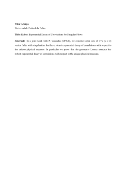
FIG. 2. Frequency distribution for different values of N and
0.0ⱗ ␻ j ⱗ 2.5.
the frequencies generator used in the simulations. However,
the qualitative behavior of our results is independent of the
frequencies generator.
Next we discuss the autocorrelation function for different
bath frequencies distributions. While Secs. III A and III B
discuss the quadratic case by changing N and ␻cut, respectively, Sec. III C shows results for the sub- and super-Ohmic
cases and Sec. III D discuss the nonrandomic case.
A. Quadratic distribution: Increasing N
Figures 2共a兲 and 2共b兲 show the distribution ␳共␻ j兲 for N
= 10 and N = 40, respectively. Clearly it can be observed that
many frequencies are missing in the interval of interest. This
characterizes a highly structured environment, which is a direct consequence of the finite number of oscillators. As the
number of oscillators increases to N = 360 and 3000, ␳共␻ j兲
approaches very slowly to a continuous function with a quadratic dependence on ␻. The distributions shown in Fig. 2
are given in the interval 0.0ⱗ ␻ j ⱗ ␻cut 共⌬␻ j ⬃ 2.5兲, with the
cutoff at ␻cut = 2.5. We refer to them as the low distribution.
For a later purpose we will refer to the case ␻cut = 4.0 共1.5
ⱗ ␻ j ⱗ 4.0兲 as the high distribution. Observe that we always
keep ⌬␻ j ⬃ 2.5 constant. It is also important to mention that
in the low distribution the frequency range from the environment includes the system frequency ␻0, i.e., includes ␻ j ⬃ 1.
However, in the high distribution all frequencies are larger
than ␻0. This will be important in Sec. V.
Figure 3 shows the time dependence of the normalized
autocorrelation function CN共t兲 for different values of N and
␻cut = 2.5. We observe that for low values of N 共=5, dashed
line兲, CN共t兲 oscillates more or less regularly around zero,
without decreasing its amplitude. This means that any value
of CN共t兲 obtained for a given time, will be repeated over and
over again for other times. The time of these repetitions is
the Poincaré recurrence time. In other words, the value of
CN共t兲 at a given time represents the “physical state” of the
discrete bath at that time. Therefore we expect that this
“physical state” is reached again and again, following the
Poincaré times.
FIG. 3. Normalized correlation function CN共t兲 for some values
of N and 0.0ⱗ ␻ j ⱗ 2.5.
As N increases the amplitude of the oscillations of CN共t兲
decreases. Compare N = 5 共dashed line兲 with N = 1000 共dotted
line兲 and N = 10 000 共full line兲 in Fig. 3. For times t ⲏ 10,
N = 1000, and N = 10 000, CN共t兲 starts to oscillate inside the
“fluctuation region” 共FR兲 关10兴. This region is shown in Fig. 3
with two horizontal straight lines. In such cases, CN共t兲 decays initially very fast and then remains inside the FR. For
values of CN共t兲 inside the FR region 共for t ⲏ 10 in Fig. 3兲, the
Poincaré recurrence times are small and CN共t兲 is repeated
over and over again. States of the discrete bath related to
these times can be named “probable states” 关10兴, since they
appear very often. For values of CN共t兲 outside the FR region
共for t ⬃ 0.0 in Fig. 3, for example兲, Poincaré recurrence times
are enormously large and it is very difficult to observe the
repetition of such values of CN共t兲 for the finite integration
times. States of the discrete bath related to these times can be
named “improbable states.” For large values of N the initial
states from Fig. 3 共t ⬃ 0.0兲 belong to such improbable states.
For Markovian processes the FR should go to zero for
N → ⬁ and t → ⬁. Therefore, from the analysis of this section
we say that the dynamics of the system coupled to the discrete bath with low frequencies is almost a non-Markovian
process, independent of N.
B. Quadratic distribution: Going to higher frequencies
In this section we study the autocorrelation function by
increasing the cutoff frequency. In fact we “move” the
distribution to higher frequencies keeping the frequency interval fixed by ⌬␻ j ⬃ 2.5. We use values of N = 10, 20,
50, 100, 1000, 10 000. The qualitative behavior of ␳共␻ j兲 and
the frequencies generator are exactly the same as in Sec.
III A. Figure 4 shows the semilogarithmic plot of the FR as a
function of ␻cut for different values of N. In all of the following simulations we determined the FR using the time
interval ⌬t = 关400, 50 000兴, independent of N. Therefore, we
extracted an initial transient of around 400. The choice if this
time interval allows us to obtain all relevant variations of FR.
In Fig. 4 we observe that the FR decreases when the ␻cut
increases, meaning that the Markovian limit could be
reached by increasing the mean bath frequencies. We also
observe the expected result that the FR decreases when N
increases. In general the autocorrelation function goes to
zero for higher frequencies and for N → ⬁. Only in this limit
031126-4
DISSIPATION AND TRANSPORT DYNAMICS IN A …
N=10
N=20
N=50
N=100
N=1000
N=10000
0.1
N=10
N=20
N=50
N=100
N=1000
N=10000
0.1
FR
1
FR
PHYSICAL REVIEW E 78, 031126 共2008兲
0.01
0.01
0.001
0.001
0.0001
2.5
3
3.5
4
ωcut
4.5
5
5.5
0.0
our discrete bath behaves like an usual Markovian Ohmic
heat bath. Any bath discreteness induces finite values for the
FR and, consequently, the non-Markovian motion.
In this section we discussed the case when the distribution
“moves” to higher frequencies keeping the frequency interval fixed by ⌬␻ j ⬃ 2.5. We could obviously discuss the case
when only ␻cut increases keeping the lower frequency close
to zero. However, if we do so, for any new value of ␻cut the
interval ⌬␻ j increases and the discreteness of the bath
changes, i.e., the density of frequencies will decrease as ␻cut
increases. Since our interest is to study the dynamics by increasing N, without decreasing the frequency density, we do
not discuss this case here.
C. From sub-Ohmic to super-Ohmic baths
To discuss the bath discreteness for other types of distributions, we consider the cases for which the spectral density
has the form J共␻兲 = ␻s, with 0 ⬍ s 艋 2 关5兴. For s = 1 the quadratic frequency distribution discussed above is recovered.
For s ⬍ 1 we have the sub-Ohmic case where lower frequencies in the allowed frequency interval have a bigger contribution when N → ⬁. For s ⬎ 1 we have the super-Ohmic case
where higher frequencies in the allowed frequency interval
have a larger contribution when N → ⬁. Nonintegral values
of s correspond to fractal environments 关5兴. Figure 5 shows
the semilogarithmic plot of the FR as a function of s for
different values of N and ␻cut = 2.5. In general the FR decreases as s increases, showing that the super-Ohmic case is
N=10
N=20
N=50
N=100
N=1000
N=10000
FR
0.1
0.01
0.001
0.0
0.5
1.0
s
1.0
1.5
2.0
s
FIG. 4. Fluctuation range as a function of ␻cut for s = 1.
1
0.5
1.5
2.0
FIG. 5. Fluctuation range as a function of s for the low distribution 0.0ⱗ ␻ j ⱗ 2.5.
FIG. 6. Fluctuation range as a function of s for the high distribution 1.5ⱗ ␻ j ⱗ 4.0.
“more Markovian” than the sub-Ohmic case. Besides N
= 1000, 10 000, all other curves have the same qualitative s
dependence. The reason for this distinct behavior is the consequence of frequencies close to zero. Since the interval of
allowed bath frequencies is 0.0ⱗ ␻ j ⱗ 2.5, when N increases
from 100 to 10 000, the number of frequencies close to zero
increases significantly. These close to zero frequencies make
the FR increase, the motion is strongly non-Markovian and
the qualitative behavior of FR as a function of s changes. We
observe that for s ⱗ 0.5, all of the values of the FR for N
= 10 000 are higher when compared to N = 1000. Since in the
sub-Ohmic distribution lower frequencies have a larger contribution, means that close to zero frequencies become more
probable to occur. As a consequence the values of FR increase very much when s decreases. These close to zero frequencies change the qualitative behavior of the FR for N
= 100, 10 000.
As the cutoff frequency increases, the zero frequencies are
not present anymore and the above distinct effect observed
for N = 100→ 10 000 should disappear. Figure 6 shows the
FR as a function of s when ␻cut ⬃ 4.0. Clearly we realize that
the FR now decreases in the transition N = 100→ 10 000,
showing that the anomalous effect due to the zero frequencies disappears Different from Fig. 5, here the FR is almost s
independent, but still N dependent.
D. Nonrandomic distributions
Nothing essentially new occurs for nonrandomic distributions when compared to the last two sections. Basically, as
before, the autocorrelation function goes to zero for N → ⬁,
t → ⬁ and for higher distributions. If we consider equally
spaced frequencies, for example, at some specific times 共the
Poincaré recurrence times兲 we observe the constructive interference 共full recurrences兲 of the autocorrelation function. The
autocorrelation function has well-defined peaks at welldefined times. As N increases, the maxima of these peaks
decrease and the times for full recurrences increase. Between
these well time localized peaks the autocorrelation function
approaches zero as N → ⬁. Physically this example could
correspond to the system coupled to a classical resonator
where a discrete number of modes is allowed 共the discrete
bath兲. The modes are usually integer multiples of the funda-
031126-5
PHYSICAL REVIEW E 78, 031126 共2008兲
JANE ROSA AND MARCUS W. BEIMS
mental frequency. From the quantum point of view this could
correspond to the interaction of atomic levels with a quantum
cavity composed of finite modes 关16兴.
ET
0.02
ES
(a)
E 0.01
IV. ENERGY TRANSFER DYNAMICS (F = 0)
EO
There are two distinct physical situations where the energy transfer can be discussed: 共i兲 The energy redistribution
between system, environment, and interaction in case the
particle stays inside one ratchet potential well, and 共ii兲 the
energy redistribution in case the particle is transferred from
one ratchet potential well to another. These situations can be
interpreted, respectively, as the classical analogous of the
much more complicated quantum dynamics, for example, the
intramolecular redistribution and intermolecular charge
transfer 关9兴. The particle staying inside one ratchet potential
well would correspond to the charge staying inside one molecule. The particle being transferred from one ratchet potential well to another, would correspond to the charge being
transferred from one molecule to another. Because of the
analogy, the above two physical situation are called here the
intrawell energy redistribution and the interwell particle
transfer, respectively. This is just an analogy and it is not our
intention to connect the classical results with the quantum
problem of molecules mentioned above.
In this section the two distinct physical situations mentioned above are briefly discussed. To do so, energy exchange from just one trajectory and one environment realization is considered in Secs. IV A and IV B. In Sec. IV C the
hopping probability is analyzed over 800 environment realizations. We used low distributions for the environment frequencies in Sec. IV A and IV B, and high distributions in
Sec. IV C.
A. Intrawell energy redistribution
Initial conditions for the particle are X共0兲 = 0.0, Ẋ共0兲
= 0.2, and the scaled coupling is ␥ j = 0.1. For 1 艋 N ⱗ 10 the
system particle is continuously exchanging energy with the
finite bath. Essentially the particle is oscillating inside one
ratchet potential well keeping for itself most of the total energy with little variations.
Figures 7共a兲 and 7共b兲 show the case of the system-plus-15
oscillators. The frequency 共for times t ⱗ 670兲 of the energy
exchange between system and environment is ␻slow ⬃ 0.035.
Different from the cases with low values of N, near t ⬃ 670
the system abruptly loses one-half of its energy to the environment 关mostly to the oscillators with lower frequencies,
see Fig. 7共b兲兴. The initial energy lost by the particle is not fed
back for the integrated time and dissipation effects appear. It
is obvious that if we integrate until t → ⬁ the energy must
return to the particle due to the finite bath and the Poincaré
recurrence times. However, since in the real world we are
always restricted to finite times, the dissipation process described in this section is of real interest.
For N → ⬁ the system energy should be mostly transferred
to the environment, and only fluctuations are expected. This
can be observed in Fig. 8 for N = 360. After reaching the limit
situation of equilibrium 共at t ⬃ 1100兲, system and environ-
0
EI
0
1
2
3
103 t
EO
0.008
(b)
0.004
0
1.5
ωj
2.5
1
0
3
2
103 t
FIG. 7. Time evolution of separated energies: 共a兲 The system ES,
oscillators EO, interaction EI, and total ET for N = 15 oscillators and
共b兲 details of the energy for each of the 15 oscillators.
ment exchange energy while the interaction energy is close
to zero. As expected, for an environment composed of many
oscillators, most of the energy is transferred from the system
into the environment. The frequency of the energy exchange
between ES and EO is not well defined and only fluctuations
in ES are observed. Following the discussion of Sec. III A,
we can mention that the system states at t ⱗ 1100 are improbable states with very large Poincaré recurrence times, while
the states for 1100ⱗ t ⱗ 15⫻ 103 are the probable states with
small Poincaré times.
B. Interwell particle transfer
Another aspect of the energy transfer dynamics occurs in
cases when the particle is transferred from one ratchet potential well to another. At t = 0 the particle receives enough energy 共ES ⬃ 0.0346兲 to transpose the peak of the ratchet barrier, with potential energy close to ⬃0.0323. As it moves
over the ratchet potential wells, it will “fall” into one ratchet
ET
0.02
EO
E 0.01
360 oscillators
ES
0
EI
0
5
10
15
103 t
FIG. 8. Time evolution of separated energies: The system ES,
oscillators EO, interaction EI, and total ET for N = 360 oscillators.
031126-6
DISSIPATION AND TRANSPORT DYNAMICS IN A …
0.04
20 oscillators
ET
ES
0.01
0.03
PHYSICAL REVIEW E 78, 031126 共2008兲
0
0.02
E
-0.01
0.01
0
100
200
300
EO
0
EI
-0.01
0
2
4
6
103 t
FIG. 9. Time evolution of separated energies: The system ES,
oscillators EO, interaction EI, and total ET for the case of the transferred particle and N = 20.
well due to damping and dissipation effects. For illustrative
purposes the scaled coupling considered here is weaker 共␥ j
= 0.03兲, and the initial conditions for the particle are X共0兲
= 0.0 and Ẋ共0兲 = 0.263.
In Fig. 9 the time evolution of the energies is shown for
the case of N = 20 oscillators. The initial energy is assumed to
be higher when compared with the preceding section, and the
particle will transpose 共to the right兲 two ratchet potential barriers. Since the coupling strength between system and environment is weaker, dissipation effects are expected to appear
only for longer times. The integrated time for Fig. 9 is therefore longer. All other parameters are the same as from the
preceding section. The inset of Fig. 9 shows details of environment and interaction energies for t 艋 300.
In order to discuss better the energy transfer dynamics, it
is important to look simultaneously at what happens to the
trajectory in position and phase space, shown in Fig. 10. For
times 0.0艋 t ⱗ 22, the particle moves to the right 关Ẋ共0兲
⬎ 0.0兴 over two ratchet potential wells 共remember, the period
of the ratchet wells is 1.0兲 and, due to dissipation effects of
the 20 oscillators, it “falls” into the well localized around the
minimum X = 2.0 and oscillates there for times 22ⱗ t ⱗ 101.
As the particle jumps over the two ratchet wells, energy is
stored into the environment which is now in a kind of “excited state” with mean energy around 0.0075. This can be
observed in the inset of Fig. 9 for t ⱗ 101. The same happens
2.5
2
1.5
X
1
0.5
(b)
(a)
0
0
100
200
300
t
400
-0.3
0
.
X
0.3
FIG. 10. Phase-space trajectory for N = 20 showing 共a兲 time dependence of the position of the particles and 共b兲 the trajectory in
phase space.
for the interaction energy but for negative values. For t
⬃ 101 the energy stored in the environment is transferred
back to the particle and it jumps back 共to the left兲 one ratchet
well, oscillating around X = 1.0 and staying there for the
whole integrated time 共see Fig. 10兲.
As the particle jumps back the last one ratchet well, the
environment decays to the “lower excited state” with mean
energy around 0.0025. See the environment energy for t
ⲏ 101 in the inset of Fig. 9. This remaining energy inside the
environment is not enough to make the particle jump another
ratchet well. Therefore, the particle stays inside the ratchet
well centered around X = 1.0 for the whole integrated time.
For times 101ⱗ t ⬍ 6 ⫻ 103, the system energy is slowly
transferred into the environment. As a consequence, the particle inside the ratchet well is slowly losing its energy, which
is manifested by the width of the trajectory in Fig. 10共b兲.
For 1 艋 N ⱗ 27 the environment affects the particle
through two different processes. First, the environment is
damping the motion of the particle, making it “to fall” into
the ratchet potential well and to stay there for a brief time.
Remember that for t = 0 the particle received enough kinetic
energy to transpose the ratchet barrier. Second, the environment may inject energy back into the system, transferring the
particle from one ratchet well to another. This is called the
“jump effect” or environment-induced transfer. For the same
trajectory this effect may occur many times. Increasing the
number of oscillators the “jump effect” will disappear 共for
N ⲏ 27兲 and only dissipation and damping effects remain. So,
only for N ⲏ 27 the particle will lose enough energy to the
environment in order to “fall” into one ratchet potential well,
staying there for the whole integrated time.
C. Hopping probability
Although results from the preceding section are shown for
just one trajectory, the effect of the environment-induced particle transfer is observed for many trajectories and is a common phenomenum for low values of N. This is shown in this
section by calculating the hopping probability between many
wells. Due to the environment-induced transfer, particles
may jump to the right and to the left. Since we have many
wells, an adequate way of quantifying the hopping probability is to count how many times nr共nl兲 the particle jumps to a
right 共left兲 ratchet well. The quantity nr / nt 共nl / nt兲 gives us
the normalized number of right 共left兲 jumps, where nt = nr
+ nl. This way of quantifying the movement of particles allows us to analyze the decay of the hopping probability
along the whole periodic structure.
Figure 11 shows the distribution of the right jump probability ␳共nr兲 after an integration time up to t = 5000 and over
800 realizations of the environment variables. Initial conditions for the particle are X共0兲 = 0.0 and Ẋ共0兲 = 0.2633, the
coupling is ␥ j = 0.1, and the high distribution is used. The
idea here is to observe the effect of the finite environment on
the motion of the particle which initially has enough kinetic
energy to transpose all ratchets potentials. For N = 0 共no environment兲, for example, we suppose that the particle has
enough kinetic energy to transpose the first ratchet well 关to
the right, since Ẋ共0兲 ⬎ 0兴. As a consequence, it will transpose
031126-7
PHYSICAL REVIEW E 78, 031126 共2008兲
JANE ROSA AND MARCUS W. BEIMS
0.3
0.16
(a) N=1
1
(b) N=5
0.12
Probabilities
0.2
0.08
0.1
0.04
0
0
0
100
200
300
400
500
0
100
200
300
400
500
0.1
0.01
0.3
0.12
(c) N=30
(d) N=360
0.001
0.2
1
0.08
ρ(nr)
Pr(N)
Pl(N)
10
100
N
0.1
0.04
0
FIG. 12. Total left 共⫻兲 and right 共䊊兲 normalized jump probabilities. Dashed and solid lines are the corresponding fitted curves.
0
0
100
200
300
400
500
0
10
20
30
40
nr
FIG. 11. Distribution of the right jump probability for 共a兲 N = 1,
共b兲 N = 5, 共c兲 N = 30, and 共d兲 N = 360.
all wells since no dissipation and damping effects are
present. For the integrated time and for each realization, the
particle transposed 494 ratchet wells, i.e., the particle
reached X共5000兲 ⬃ 494. Therefore, for N = 0 we have nr
= 494 and nl = 0 for each realization. Now, take the particle
above 共same initial conditions and same integrated time兲 but
with N = 1. In this case, the particle may lose part of its
kinetic energy due to the “collisions with the environment
composed of one oscillator.” As a consequence, for some
realizations the particle may not reach X ⬃ 494 as before.
This is shown in Fig. 11共a兲, where the pronounced peak with
probability ⬃0.3 is observed near nr = 494 共X ⬃ 494兲. It
means that most of the trajectories are still jumping to the
right over 494 wells. Such a big number of right jumps is
obvious because damping and dissipation effects are expected to be small for N = 1, and the particle is more or less
“free” to move over the ratchet wells. We also see in Fig.
11共a兲 some finite probabilities along lower values of right
jumps 共0 ⬍ nr ⱗ 200兲. Such low values of nr cannot be a consequence of dissipation and damping effects, because they
are small for N = 1. Low values of nr are the consequence of
left jumps, or the environment-induced transfer observed in
the preceding section. For N = 5, dissipation and damping
effects start to affect more the dynamics, and the number of
initial conditions which reach X ⬃ 494 is lower 关see Fig.
11共b兲兴. As the number of oscillators increase to N = 30 关Fig.
11共c兲兴, damping and dissipation start to be stronger,
environment-induced transfers get smaller, and the final right
jump probability approximates 共for N = 360兲 a kind of Gaussian distribution around nr ⬃ 20 wells 关see Fig. 11共d兲兴.
A more qualitative way to observe this is to study the total
right Pr共N兲 关or left Pl共N兲兴 normalized jump probabilities as a
function of N. They are obtained by simply adding, for a
given N, all values of nr 共or nl兲 over the 800 realizations, and
dividing them by 494⫻ 800, which is the maximal value of
nr ⫻ 800 obtained for N = 0. Figure 12 shows Pr共N兲 and Pl共N兲
as a function of N. Both normalized probabilities decrease
very fast as N increases. However, the left jump probability,
consequence of the environment-induced transfer, decreases
much faster and for N ⬃ 30 it is close to zero, as expected
from results of the preceding section. We fitted both curves
by an inverse power law. It can be observed that Pl共N兲 is
well fitted 共dashed line兲 by an inverse power law which goes
with exponent ⬃1.04. For Pr共N兲 however, we clearly see two
distinct regions where the exponent of the power law is different. The first for 1 ⬍ N ⱗ 30, obeys the inverse power law
with exponent ⬃0.635 and the second region, for N ⲏ 40,
follows a power law with exponent ⬃0.163. This means that
for 1 ⬍ N ⱗ 30 the right jump probability Pr共N兲 is mainly
affected by the left jump probability Pl共N兲, i.e., the
environment-induced transfer to the left. As we have shown
in the preceding section, this is a typical characteristic of
discrete baths. In the region N ⲏ 40, Pr共N兲 is affected by real
damping and dissipation effects.
Concluding this part we showed that, for the given particle with initial velocity 共to the right兲 and 800 environment
realizations, the left jump probability vanishes as N increases, showing that the environment-induced transfer 共to
the left兲 is destroyed for higher values of N. Moreover, we
showed that the right jump probability also decreases as N
increases, and that for N = 360 it has a stationary Gaussian
distribution along the periodic structure. For future reference,
we call to attention that for N = 360 the transport of particles
along the periodic structure can be destroyed by damping
and dissipation, while for low values of N, environmentinduced transport is also important. Similar results from this
section are obtained when we start with the negative velocity
Ẋ = −0.2633. Just change nr by nl, and vice versa. It is also
worth mentioning that 1 / N plays the role of the bath temperature T. Since the total energy is equal in all simulations,
the mean energy and oscillator from the discrete bath will
decrease with N, which corresponds to a bath that becomes
colder. Therefore, our escape rate decreases with a power
law in 共N ⬀ 1 / T兲 while the usual escape rate 关5兴 decreases
exponentially with 共1 / T兲.
V. ENVIRONMENT-DEPENDENT RATE OF DISSIPATION
(F = 0)
Although the results from Secs. IV A and IV B are important to describe energy transfer dynamics for particular trajectories, they are not sufficient to make statements about
general laws of the energy transfer dynamics. In order to do
this, in this section the energy transferred from system to
environment is studied for an ensemble of particles for the
031126-8
DISSIPATION AND TRANSPORT DYNAMICS IN A …
0.010
<ES>
(a)
1000
0.0015
x
y
0.4
z
ν
0.2
{
|
}
0.001
10000
t
PHYSICAL REVIEW E 78, 031126 共2008兲
power law
exponential
0.0010
(b)
<ES>
N = 500
0.0005
0.0
(a)
1000
10000
(a)
0
t
200 400
power law
exponential
N
0.0195
FIG. 13. 共a兲 Log-log plot of the time evolution of averaged
system energies 共over 800 trajectories兲 and adjusted curves for N
= 2共¬兲, 20共−兲, 60共®兲, 140共¯兲 180共°兲 and 360共±兲 and 共b兲 values
of the exponent ␯ from Eq. 共9兲 for low distribution 共squares兲, and
high distribution 共circles兲.
<ES>
N = 500
0.0194
(b)
intrawell case from Sec. IV A. An average over 800 trajectories is taken. The rate of energy lost by the system is analyzed as N increases. The scaled coupling between system
and environment is ␥ j = 0.1.
Figure 13共a兲 shows the log-log plot of the time evolution
of the average system energy 具ES典 for different values of N.
Only late times 共t ⬎ 1000兲 are discussed. For N = 2, no decay
is observed for the mean system energy and dissipation is
considered zero. For N 艌 20 decay is observed in all cases.
We checked the energy decay 共over many initial conditions兲
for all values of N ⬍ 20 and observed that dissipation effects
always appear in the interval 10ⱗ N ⱗ 20. This also agrees
with results from the preceding section where dissipation
effects start to appear for about N ⬃ 15. The goal now is to
find the time decay law for the system dissipation rate for
late times. Figure 13共a兲 shows that the average of the decay
rate is linear in the log-log plot. Therefore, the system energy
can be well adjusted by an inverse power-law curve given by
具ES典 ⬀ t−␯ ,
共9兲
where ␯ is the exponent which determines the dissipation
rate. In Fig. 13共a兲 the adjusted curves are plotted for each
value of N, demonstrating that the dissipation decay rates
really obeys an inverse power law. The dependence of ␯共N兲
for the low distribution is shown in Fig. 13共b兲 共square
points兲. It can be observed that the dissipation decay rate
increases as the number of oscillators increases from N = 2 to
N = 140. In this interval, the energy flows faster from the
system into the environment as N increases. For N = 140, the
energy decay rate reaches a maximum and decreases a little
for N = 180, approaching a value near 0.31 for N = 500. The
maximum observed for N = 140 means that, for this number
of oscillators, the environment receives more likely the energy from the system. Such an effect is related to the low
distribution which includes values of ␻ j 艋 1. To explain this
we must call to attention that the rate of transferred energy is
higher for ␻ j ⬍ 1 than for ␻ j ⬎ 1. This is obvious when we
realize that the transferred energy ES → E j 共energy of the jth
oscillator兲 occurs more likely when ES ⬎ E j. Since the low
10000
(b)
20000
t
FIG. 14. Log-log plot of the time evolution of averaged system
energies and adjusted curves for N = 500 and 共a兲 low distribution
and 共b兲 high distribution. Black lines are results for the simulations,
dashed lines for the power-law fit, and long dashed line for the
exponential fit.
distribution includes some frequencies with ␻ j 艋 1, the number of oscillators with ␻ j ⬍ 1 can be different than the number of oscillators with ␻ j ⬎ 1 共for sufficiently low values of
N兲. In fact, it will depend on the frequency generator. A more
detailed analysis of the low frequencies distribution showed
that the number of oscillators with ␻ j ⬍ 1 are proportionally
greater for N = 140 than for N = 180 and N = 360. As a consequence, the rate of the transferred energy is expected to be
higher for N = 140, as observed in Fig. 13共b兲. When another
frequency generator is used, the maximum observed for N
= 140 could occur for other values of N. However, such
maximum will only appear for finite baths. The above maximum will disappear when all oscillator frequencies obey ␻ j
⬎ 1. The points 共circles兲 from Fig. 13共b兲 exemplifies this. It
shows the values of ␯ 关from Eq. 共9兲兴 as a function of N for
the high distribution 共1.5ⱗ ␻ j ⱗ 4.0兲. In this case the value of
the exponent is close to zero and increases very slowly with
N. Therefore, energy decay rates are higher in the low distribution case. The empty circle in Fig. 13共b兲 for N = 500 is
explained below.
Comparing the above results with the analysis of discrete
baths from Sec. III, we conclude that we have two reasons
why we see the energy power-law decay: 共1兲 The cutoff frequency distribution is too small and/or 共2兲 the values of N are
not large enough. In order to check this we show in Fig. 14
more details of the energy decay for N = 500 for the low 关Fig.
14共a兲兴 and high 关Fig. 14共b兲兴 distribution cases. Black lines
are results for the simulations, dashed lines for the powerlaw fit, and long dashed line for the exponential fit. While for
the low distribution we still have a power-law, for the high
distribution case the energy decay starts to approach an ex-
031126-9
PHYSICAL REVIEW E 78, 031126 共2008兲
JANE ROSA AND MARCUS W. BEIMS
0.2
0.10
0.1
0.05
0.00
J
0.0
J -0.05
-0.1
-0.10
-0.15
-0.2
0
100
200
N
300
-0.20
400
0
10
20
30
40
50
N
FIG. 15. Current J as a function of N for different values of the
amplitude of the external force: F = 0.05 共䊐,䊏兲, F = 0.1 共䉱,䉭兲, F
= 0.5 共쎲,䊊兲. Filled symbols for the low distribution 共which includes
␻ j 艋 1.0 and with ␻cut ⬃ 2.5兲, and empty symbols for the high distribution 共where all ␻ j ⬎ 1.0 and ␻cut ⬃ 4.0兲.
ponential decay. This transition from power-law to exponential energy decay occurs very slowly and only when the fit is
done for later times. Observe that the time interval for the fits
from Figs. 14共a兲 and 14共b兲 is different. In fact, when we fit
the energy decay for the low distribution 关Fig. 14共a兲兴, but
using later times 共t ⬎ 10 000兲, we still get the power law.
This is not shown. However, for the high distribution case
the differences between the power law and exponential
curves in Fig. 14共b兲 are very small, but convincing. The last
point 共empty circle兲 in Fig. 13共b兲 for N = 500 comes from the
power-law fit from Fig. 14共b兲. In fact, for this point we
should already use the exponential decay, but the differences
between both are very small. The main point is that for
higher distributions and later times the exponential decay is
slowly recovered. As the number N increases the computer
CPU times for simulations increases very much. This is the
reason we did not consider higher values of N.
For short times 共t ⬍ 1000兲, a kind of stretched exponential
decay rates were found. However, since in our analysis we
always start at t = 0 with a nonequilibrium situation, such
decay rates are not discussed here.
VI. CURRENT (F Å 0)
Finally we discuss the transport along the periodic structure by turning on the external force F. The asymmetry of
the ratchet potential, together with the external force, allow
particles to move in a preference direction inducing the net
current. In this section we analyze the current as a function
of the number of oscillators. A high efficiency of the current
in the ratchet device is a very desirable quantity, then it will
affect directly the transport.
The current J along the ratchet can be defined as the time
average of the average velocity over an ensemble of initial
M
conditions. It is calculated from J = M1 兺i=1
vi, where the sum
is over M different times ti and vi is the average velocity at
the time ti over the 800 initial conditions. Figure 15 shows
the current as a function of N for different values of the
amplitude of the external force F = 0.05 共䊐,䊏兲, F = 0.1
共䉱,䉭兲, F = 0.5 共쎲,䊊兲. Filled symbols are results for the low
distribution and empty symbols are results for the high dis-
FIG. 16. Current reversal obtained as a function of N. This curve
shows in more details the result from Fig. 15 for F = 0.1.
tribution. The coupling intensity is ␥ j = 0.1 and the frequency
of the external field is ␻ = 0.035.
First observation in Fig. 15 is that the most relevant currents occur, for both distributions, at F = 0.1. For N = 2 these
currents are negative 关see the 共䉱,䉭兲 points兴. As N increases,
the current for the high distribution keeps its values inside
the interval 共−0.1, −0.2兲. For the low distribution case we
observe current reversal occurring in the interval 5 ⱗ N ⱗ 30.
This is shown in more details in Fig. 16. This interval is
approximately the interval for which dissipation and bathinduced transfer effects from Secs. IV B and IV C appear
共see text related to Fig. 9兲. Since the environment can induce
transfer in another direction than the original, the average
over the velocity decreases and the current also decreases. In
fact, environment-induced transfer may decreases the efficiency of the current. In our case we can say that the bathinduced particle transfer decreases the current in the interval
2 ⱗ N ⱗ 20 and contributes for the current reversal. The phenomenon of current reversal is common to appear in ratchets
when parameters such as the particle mass, viscosity, amplitude of the external force, and temperature are varied
关38,39兴. We show here that current reversal occurs when N
increases.
Another interesting observation from Fig. 15 is the saturation effect. For F = 0.05 the current is almost zero for any
N, it increases until the maximum is reached at F = 0.1 共we
calculated the current for other intermediate values兲 and then
J returns to be close to zero for higher values of F. This is
shown more clearly in Fig. 17, where the current is plotted as
a function of F for different values of N. In other words, the
mobility of particles, which can be defined as J / F, has a
maximum at F = 0.1. Such saturation as a function of the
external amplitude was also observed in the usual treatment
of ratchets using the Langevin approach 关38–40兴. At the
maxima F = 0.1, current reversal is observed by changing
from low to high distributions 共compare black and gray
circles in Fig. 17兲. Just for comparison, the 共⫻兲 points plotted in Fig. 17共d兲 are results obtained by integrating the
Langevin equation. The dissipation coefficient used in the
Langevin simulation is obtained from the high distribution
case from Fig. 13共b兲.
VII. CONCLUSIONS
While the transport of Brownian particles in periodic
structures has been the subject of interest in many areas
031126-10
DISSIPATION AND TRANSPORT DYNAMICS IN A …
PHYSICAL REVIEW E 78, 031126 共2008兲
0.2
(a) N=60
(b) N=180
(c) N=270
(d) N=360
0.0
-0.2
0.2
J
0.0
-0.2
0.1
0.2
0.3
F
0.4
0.5
0.1
0.2
0.3
0.4
0.5
FIG. 17. Current J as a function of the external amplitude F for
different values of N. Black 共gray兲 circles are results for the low
共high兲 distribution. The points ⫻ in 共d兲 are results using the Langevin equation.
关30–35兴, system-plus-environment models have also become
popular due to their ability to describe dissipation in classical
关1–3兴 and quantum mechanics 关3–6,9兴. Usually in such models the environment is well described by the thermal bath
composed of infinite uncoupled harmonic oscillators. However, as mentioned in the introduction, there is a reasonable
number of systems in nature which are coupled to finite
baths 关16–19,21,22兴. This work analyzes the situation of particles in a ratchet 共the system兲 coupled to the finite number N
of oscillators 共the discrete bath兲. In particular, we study the
effect of changing N on the transport of particles and hopping probabilities along the ratchet; the energy transfer dynamics between system and the discrete bath; and the dissipation rate of the system.
In Sec. III we discuss the autocorrelation function for different bath frequencies distributions. While Secs. III A and
III B discuss the quadratic case by changing N and ␻cut, respectively, Sec. III C shows results for the sub- and superOhmic cases and Sec. III D discuss the nonrandomic case.
The main observation is that the fluctuation range 共FR兲 from
the autocorrelation function goes to zero only for higher distributions and for N → ⬁. This suggests that the Markovian
limit cannot be obtained for discrete baths with low values of
N and low distributions.
For the intrawell case, discussed in Sec. IV A, the particle
stays inside one ratchet potential well and first manifestation
of dissipation were observed for environments composed of
10ⱗ N ⱗ 20 oscillators. For lower values of N the initial energy is always fed back into the system, which is the consequence of small Poincaré recurrence times. As the number of
oscillators increases, dissipation and damping effects become
stronger and most of the system energy is transferred into the
environment and only fluctuations in the system energy remain. This is confirmed by results shown in Fig. 8 for N
= 360. The relation of such results with specific properties of
the finite bath 共such as the Poincaré recurrence times兲 was
also discussed.
An interesting situation appears for low values of N in the
interwell case, where the particle has enough energy to jump
over the periodic barriers. Each time the particle jumps over
one ratchet barrier, moving away from 共closer to兲 the initial
ratchet well, the mean energy of the environment increases
共decreases兲. The environment is in a kind of “excited state.”
This stored energy in the environment is used to transfer the
particle back from one ratchet well to another. An
environment-induced particle transfer is observed. For low
values of N the environment acts 共for the intrawell and interwell cases兲 actively on the system by transferring enough
energy to the particle in order to change qualitatively its
motion. This effect will disappear as the number of oscillators increases 共N ⲏ 27兲 and only dissipation and damping effects will remain. Results for the hopping probabilities along
the ratchet confirm these results. The total right and left jump
probabilities decrease as N increases. Important to mention is
that for N ⲏ 30 the transport of particles along the periodic
structure is destroyed due to damping and dissipation, while
in the case of low values of N 共1 ⬍ N ⱗ 27兲, the transport is
affected by the environment-induced transfer. We mention
that this is only possible in finite environments. For an ensemble of particles the dissipation decay rate is shown to
obey, for the low and high distributions, an inverse power
law for late times. This behavior is typical of discrete baths
which for low and intermediate values of N is always nonMarkovian. The exponential decay is recovered for high bath
frequencies distribution and for high values of N, where the
Markovian limit is expected.
Finally we discussed the case of net current induced by
the additional external oscillating field with intensity F. The
current along the ratchet is studied as a function of N and for
different values of F. We showed that a maximum in the
mobility of the particles is obtained for F = 0.1 for both, low
and high distributions. This result is independent of N for
N ⲏ 27. For the low distribution case and F = 0.1, decreasing
the values of N the current decreases, changes its sign, and
current reversal is observed. Therefore, when the system is
coupled to the modulated environment the mobility of particles may change its direction. Current reversal is also found
共for F = 0.1兲 by switching from low to high distribution in the
environment.
ACKNOWLEDGMENTS
J.R. and M.W.B. thank CNPq and FINEP, under project
CTINFRA-1, for financial support and J. A. O. Freire for
helpful discussions.
031126-11
PHYSICAL REVIEW E 78, 031126 共2008兲
JANE ROSA AND MARCUS W. BEIMS
关1兴 P. Ullersma, Physica 共Utrecht兲 32, 27 共1966兲.
关2兴 R. Zwanzig, J. Stat. Phys. 9, 215 共1973兲.
关3兴 E. Cortés, B. J. West, and K. Lindenberg, J. Chem. Phys. 82,
2708 共1985兲.
关4兴 A. O. Caldeira and A. J. Leggett, Phys. Rev. Lett. 46, 211
共1981兲.
关5兴 U. Weiss, Quantum Dissipative Systems 共World Scientific, Singapore, 1999兲.
关6兴 N. G. van Kampen, Stochastic Processes in Physics and
Chemistry 共North-Holland, Amsterdam, 1992兲.
关7兴 H. J. Carmichael, Statistical Methods in Quantum Optics I
共Springer, Berlin, 1999兲.
关8兴 W. T. Strunz, L. Diósi, N. Gisin, and T. Yu, Phys. Rev. Lett.
83, 4909 共1999兲.
关9兴 V. May and O. Kühn, Charge and Energy Transfer Dynamics
in Molecular Systems 共Wiley-VCH, Berlin, 2000兲.
关10兴 P. Mazur and E. Montroll, J. Math. Phys. 1, 70 共1960兲.
关11兴 V. Wong and M. Gruebele, Chem. Phys. 284, 29 共2002兲.
关12兴 F. Q. Potiguar and U. M. S. Costa, Physica A 342, 145 共2004兲.
关13兴 A. A. Budini, Phys. Rev. E 72, 056106 共2005兲.
关14兴 J. Rosa and M. W. Beims, Physica A 342, 29 共2004兲.
关15兴 J. Rosa and M. W. Beims, Physica A 386, 54 共2007兲.
关16兴 M. O. Scully and M. S. Zubairy, Quantum Optics 共Cambridge
University Press, Cambridge, 1997兲.
关17兴 J. M. Raimond, T. Meunier, P. Bertet, S. Gleyzes, P. Maioli, A.
Auffeves, G. Nogues, M. Brune, and S. Haroche, J. Phys. B
38, S535 共2005兲.
关18兴 P. Bertet, S. Osnaghi, P. Milman, A. Auffeves, P. Maioli, M.
Brune, J. M. Raimond, and S. Haroche, Phys. Rev. Lett. 88,
143601 共2002兲.
关19兴 A. Damjanović, I. Kosztin, U. Kleinekathofer, and K.
Schulten, Phys. Rev. E 65, 031919 共2002兲.
关20兴 H. Plohn, S. Krempl, M. Winterstetter, and W. Domcke, Chem.
Phys. 200, 11 共1995兲.
关21兴 M. Gruebele and P. G. Wolynes, Acc. Chem. Res. 37, 261
共2004兲.
关22兴 I. Burghardt, M. Nest, and G. A. Worth, J. Chem. Phys. 119,
5364 共2003兲.
关23兴 V. Bernshtein and I. Oref, J. Chem. Phys. 108, 3543 共1998兲.
关24兴 Y.-C. Lai and C. Grebogi, Phys. Rev. E 54, 4667 共1996兲.
关25兴 P. C. Rech, M. W. Beims, and J. A. C. Gallas, Phys. Rev. E 71,
017202 共2005兲.
关26兴 U. Feudel, C. Grebogi, B. R. Hunt, and J. A. Yorke, Phys. Rev.
E 54, 71 共1996兲.
关27兴 L. Wang, G. Benenti, G. Casati, and B. Li, Phys. Rev. Lett. 99,
244101 共2007兲.
关28兴 J. Rosa, C. Manchein, and M. W. Beims 共unpublished兲.
关29兴 M. O. Magnasco, Phys. Rev. Lett. 71, 1477 共1993兲.
关30兴 P. Reimann, Phys. Rep. 361, 57 共2002兲.
关31兴 S. Kohler, J. Lehmann, and P. Hanggi, Phys. Rep. 406, 379
共2005兲.
关32兴 R. D. Astumian and P. Hanggi, Phys. Today 55, 33 共2002兲.
关33兴 J. B. Gong and P. Brumer, Annu. Rev. Phys. Chem. 56, 1
共2005兲.
关34兴 C. Blomberg, Phys. Life. Rev. 3, 133 共2006兲.
关35兴 W. Neupert and M. Brunner, Nat. Rev. Mol. Cell Biol. 3, 555
共2002兲.
关36兴 J. L. Mateos, Phys. Rev. Lett. 84, 258 共2000兲.
关37兴 W. H. Press, S. A. Teukolsky, W. Vetterling, and B. Flannery,
Numerical Recipes in Fortran 共Cambridge University Press,
Cambridge, 1992兲.
关38兴 J. D. Bao, Y. Abe, and Y. Z. Zhuo, Physica A 277, 127 共2000兲.
关39兴 T. Sintes and K. Sumithra, Physica A 312, 86 共2002兲.
关40兴 L. Machura, M. Kostur, P. Talkner, J. Luczka, F. Marchesoni,
and P. Hänggi, Phys. Rev. E 70, 061105 共2004兲.
031126-12