Accepted Manuscript
A new Optical Music Recognition system based on Combined Neural
Network
Cuihong Wen, Ana Rebelo, Jing Zhang, Jaime Cardoso
PII:
DOI:
Reference:
S0167-8655(15)00039-2
10.1016/j.patrec.2015.02.002
PATREC 6164
To appear in:
Pattern Recognition Letters
Received date:
Accepted date:
5 May 2014
4 February 2015
Please cite this article as: Cuihong Wen, Ana Rebelo, Jing Zhang, Jaime Cardoso, A new Optical
Music Recognition system based on Combined Neural Network, Pattern Recognition Letters (2015),
doi: 10.1016/j.patrec.2015.02.002
This is a PDF file of an unedited manuscript that has been accepted for publication. As a service
to our customers we are providing this early version of the manuscript. The manuscript will undergo
copyediting, typesetting, and review of the resulting proof before it is published in its final form. Please
note that during the production process errors may be discovered which could affect the content, and
all legal disclaimers that apply to the journal pertain.
ACCEPTED MANUSCRIPT
Highlights
• We propose a new OMR system to recognize the music
symbols without segmentation.
• A new classifier named Combined Neural Network(CNN)
is presented.
• Tests conducted on fifteen pages of music sheets show that
the proposed method constitutes an interesting contribution to OMR.
AC
CE
PT
ED
M
AN
US
CR
IP
T
• The Combined Neural Network(CNN) offers superior
classification capability.
ACCEPTED MANUSCRIPT
1
Pattern Recognition Letters
journal homepage: www.elsevier.com
A new Optical Music Recognition system based on Combined Neural Network
a College
b INESC
of electrical and information engineering, Hunan University, Changsha 410082, China
Porto, Universidade do Porto, Porto, Portugal
CR
IP
T
Cuihong Wena,∗∗, Ana Rebelob , Jing Zhanga, Jaime Cardosob
ARTICLE INFO
ABSTRACT
Article history:
Optical Music Recognition (OMR) is an important tool to recognize a scanned
page of music sheet automatically, which has been applied to preserving music
scores. In this paper, we propose a new OMR system to recognize the music
symbols without segmentation. We present a new classifier named Combined
Neural Network(CNN) that offers superior classification capability. We conduct tests on fifteen pages of music sheets, which are real and scanned images.
The tests show that the proposed method constitutes an interesting contribution
to OMR.
c 2015 Elsevier Ltd. All rights reserved.
AN
US
Communicated by S. Sarkar
M
Keywords:
Neural network
Optical music recognition
Image processing
1. Introduction
AC
CE
PT
ED
A significant amount of musical works produced in the past
are still available only as original manuscripts or as photocopies
on date. The OMR is needed for the preservation of these works
which requires digitalization and should be transformed into a
machine readable format. Such a method is one of the most
promising tools to preserve the music scores. In addition, it
makes the search, retrieval and analysis of the music sheets easier. An OMR program should thus be able to recognize the musical content and make semantic analysis of each musical symbol of a musical work. Generally, such a task is challenging because it requires the integration of techniques from some quite
different areas, i.e., computer vision, artificial intelligence, machine learning, and music theory.
Technically, the OMR is an extension of the Optical Character Recognition (OCR). However, it is not a straightforward
extension from the OCR since the problems to be faced are substantially different. The state of the art methods typically divide
the complex recognition process into five steps, i.e., image preprocessing, staff line detection and removal, music symbol segmentation, music symbol classification, and music notation reconstruction. Nevertheless, such approach is intricate because
∗∗ Corresponding
author: Tel.: +86-13467672358;
e-mail: [email protected] (Cuihong Wen)
Fig. 1. Proposed architecture of the OMR system.
it is burdensome to obtain an accurate segmentation into individual music symbols. Besides, there are numerous interconnections among different musical symbols. It is also required
to consider that the writers have their own writing preference
for handwritten music symbols. In this paper we propose a new
OMR analysis method that can overcome the difficulties mentioned above. We find that the OMR can be simplified into
four smaller tasks, which has been showed in Figure1. Technically, we merge the music symbol segmentation and classification steps together.
The remainder of this paper is structured as follows. In Sec-
ACCEPTED MANUSCRIPT
2
tion 2 we review the related works in this area. In Section 3 we
describe the preprocessing steps, which prepare the system we
will study on. Section 4 is the main part of this paper. In this
section we focus on the music symbol detection and classification steps. We will discuss and summarize our conclusions in
the last two sections.
Fig. 2. Before Staff line removal
2. Related works
Fig. 3. After Staff line removal
CR
IP
T
edge. These four lines form a box that define the boundary of
the score area. Finally, we remove the black pixels outside the
box.
3.2. Staff line detection and removal
Staff line detection and removal are fundamental stages on
the OMR process, which have subsequent processes relying
heavily on their performance. For handwritten and scanned music scores, the detection of the symbols are strongly effected
by the staff lines. Consequently, the staff lines are firstly removed. The goal of the staff line removal process is to remove
the lines as much as possible while leaving the symbols on the
lines intact. Such a task dictates the possibility of success for
the recognition of the music score. Figure 3 is an example of
staff line removal for Figure 2.
To be specific, the staves are composed of several parallel
and equally spaced lines. Staff line height (Staff line thickness) and staff space height (the vertical line distance within
the same staff) are the most significant parameters in the OMR,
see Figure4. The robust estimation of both values can make the
subsequent processing algorithm more precise. Furthermore,
the algorithm with these values as thresholds are easily adapted
to different music sheets. In (I Fujinaga, 2004), staff line height
and staff space height are estimated with high accuracy. The
work developed in (Jaime S. Cardoso and Ana Rebelo, 2010)
presented a robust method to reliably estimate the thickness of
the lines and the interline distance.
CE
PT
ED
M
AN
US
Most of the recent work on the OMR include staff lines detection and removal (I Fujinaga, 2004; J. S. Cardoso et al.,
2009; Ana Rebelo and Jaime S. Cardoso, 2013; C. Dalitz,
2008), music symbol segmentation(F. Rossant and I. Bloch,
2007; Forns et al., 2005) and music recognition system approaches(G. S. Choudhury et al., 2000). Recently, (Ana Rebelo
et al., 2013) proposed a parametric model to incorporate syntactic and semantic music rules after a music symbols segmentation’s method. (Florence Rossant, 2002)developed a global
method for music symbol recognition. But the symbols were
classified into only four classes. A summary of works in the
OMR with respect to the methodology used was also shown in
(Ana Rebelo et al., 2012).
There are several methods to classify the music symbols,
such as the Support Vector Machines(SVM), the Neural Networks (NN), the k-Nearest Neighbor(k-NN) and the Hidden
Markov Models(HMM). For comparative study, please see
(Ana Rebelo et al., 2010). However, it is worthy to note that the
operation of symbol classification can sometimes be linked with
the segmentation of the objects from the music symbols. In (L.
Pugin, 2006), the segmentation and classification are performed
simultaneously using the Hidden Markov Models (HMM). Although all the above mentioned approaches have been shown to
be effective in specific environments, they all suffer from some
limitations. The former (Ana Rebelo et al., 2010) is incapable
of obtaining an output with a proper probabilistic interpretation
with the SVM and the latter (L. Pugin, 2006) suffers from unsatisfactory recognition rates. In this paper, we simplify all the
process and also overcome the issues inherent in sequential detection of the objects, leading to fewer errors. What is more,
we propose a new Combined Neural Network(CNN) classifier,
which has the potential to achieve a better recognition accuracy.
3. Preprocessing steps
AC
Before the recognition stage, we have to take two fundamental preprocessing steps, i.e., image pre-processing and staff line
detection and removal.
3.1. Image pre-processing
The image pre-processing step consists of the binarization
and noise removal process. First, the images are binarized with
the Otsu threshold algorithm(N. Otsu, 1979). Then we remove
the noise around the score area. The boundary of the score area
is estimated by the connect components. We find the first and
the last staff lines in the music sheet. At the same time, we
choose the minimum start point of the score area as the left
edge and the maximum end point of the score area as the right
Fig. 4. Staff Line Height and Space Height
In (J. S. Cardoso et al., 2009), a connected path algorithm
for the automatic detection of staff lines in music scores was
proposed. It is naturally robust to broken staff lines (due to lowquality digitization or low-quality originals) or staff lines as thin
as one pixel. Missing pieces are automatically completed by
ACCEPTED MANUSCRIPT
3
Fig. 6. The structure of the MLP.
the algorithm. In this work, staff line detection and removal is
carried out based on a stable path approach as described in (J.
S. Cardoso et al., 2009).
resized to 35*20 pixels and then converted to a vector of 700
binary values. At the same time, the images of the input 3 are
resized to 60*30 pixels and then converted to a vector of 1800
binary values. We give them different sizes in order to obtain
different neural networks. Later the classification of three neural networks could be combined. We choose these values in
proportion with the aspect ratio of bounding rectangles of the
symbols. The shapes of most music symbols are similar to one
of the following shapes.
4. Music symbol classification and detection
M
AN
US
This section is the main part of the paper, which consists
of the study of music symbol detection and classification. We
firstly split the music sheets into several blocks according to the
positions of the staff lines. A set of horizontal lines are defined,
which allow all the music symbols in the blocks. After the decomposition of the music image, only one block of the music
score will be processed at a time. For example, Figure 2 is a
block from a page of music sheet.
The CNN will be used as the classifier. And the detection of
the symbols are started with the method of connect components.
These will be described in the following two subsections.
CR
IP
T
Fig. 5. The structure of the CNN
PT
ED
4.1. Music symbol classification
As mentioned before, the classification of the music symbols
in this paper is based on a designed CNN. In this section, more
details about the CNN will be described.
AC
CE
4.1.1. Proposed architecture of the CNN
A theory of classifier combination of Neural Network was
discussed in(Dar-Shyang Lee., 1995). Our CNN is based on
the theory of (Dar-Shyang Lee., 1995). The main idea behind
is to combine decisions of individual classifiers to obtain a better classifier. To make this task more clearly defined and subsequent discussions easier, here we describe the architecture of
the CNN in Figure 5.
The three identity neural networks in Figure 5 will be introduced in the following subsection, each of them is a Multi-layer
Perception (shorted as MLP, see Figure 6 for detail). And the
other focus of the CNN is how the information presented in output vectors affects combined performance. This can be easily
achieved by applying different majority vote functions.
4.1.2. The Inputs
Firstly, each music symbol image is converted to a binary
image by thresholding. Then the images are resized. For input1, the images are resized to 20*20 pixels and then converted
to a vector of 400 binary values. For input 2, the images are
• 20*20: semibreve(e.g.
• 35*20: flat(e.g.
• 60*30: notes(e.g.
), accents (e.g.
),rest(e.g.
)
)
), notes flags (e.g.
).
4.1.3. Multi-layer Perceptron (MLP)
The MLP inside each of the three Neural Networks in Figure
5 is introduce in Figure 6. It is a type of feed-forward neural
network that have been used in pattern recognition problems
(F.Rosenblatt, 1957). The network is composed of layers consisting of various number of units. Units in adjacent layers are
connected through links whose associated weights determine
the contribution of units on one end to the overall activation of
units on the other end.
There are generally three types of layers. Units in the input
layer bear much resemblance to the sensory units in a classical
perceptron. Each of them is connected to a component in the
input vector. The output layer represents different classes of
patterns. Arbitrarily many hidden layers may be used depending on the desired complexity. Each unit in the hidden layer
is connected to every unit in the layer immediately above and
below.
The Multi-layer Perceptron model can be represented as
aj =
n
X
i=1
g(a j ) =
w ji xi + w j0 , j = 1, · · ·, H.
(1)
1
1 + exp(−a j )
(2)
ACCEPTED MANUSCRIPT
4
Accent
BassClef
Beam
Flat
natural
Note
NoteFlag
NoteOpen
RestI
RestII
Sharp
TimeN
TrebleClef
TimeL
AltoClef
Noise
Breve
Semibreve
M
ED
PT
CE
AC
4.1.5. Majority vote
In each neural network inside the CNN, there is one output
which represents the corresponding class of the input image.
Dots
Barlines
Table 2. Full set of the music symbols of CNN NETS 5.
vertical
lines
note
groups
dots and
note heads
AN
US
4.1.4. Database and Training
A data set of both real handwritten scores and scanned scores
is adopted to perform the CNN. The real scores consist of 6
handwritten scores from 6 different composers. As mentioned,
the input images are previously binarized with the Otsu threshold algorithm(N. Otsu, 1979). In the scanned data set, there are
9 scores available from the data set of (C. Dalitz, 2008), written
on the standard notation. A number of distortions are applied to
the scanned scores. The deformations applied to these scores
are curvature, rotation, Kanungo and white speckles, see(C.
Dalitz, 2008) for more details. After the deformations, we have
45 scanned images in total. Finally, more than ten thousand
music symbol images are generated from 51 scores.
The training of the networks is carried out under Matlab
7.8.Several sets of symbols are extracted from different musical
scores to train the classifiers. Then the symbols are grouped according to their shapes and a certain level of music recognition
is accomplished. For evaluation of the pattern recognition processes, the available data set is randomly split into three subsets:
training, validation and test sets, with25%, 25% and 50% of the
data, respectively. This division is repeated 4 times in order to
obtain more stable results for accuracy by averaging and also
to assess the variability of this measure. No special constraint
is imposed on the distribution of the categories of symbols over
the training, validation and test sets. We only guarantee that at
least one example of each category is present in the training set.
Using the above method, we train two networks which named
CNN NETS 20 and CNN NETS 5 respectively. The relevant
classes for the CNN-NETS-20 used in the training phase of the
classification models are presented in Table 1. The symbols
are grouped according to their shapes. The rests symbols are
divided into two classes, named RestI and RestII. And the relations are removed. We generate the noise examples from the
reference music scores, which have the exact positions of all the
symbols. We shift the positions a little to get the noise samples.
Some of the samples are parts of the symbols, and some are the
noises on the music sheet. In total the classifier is evaluated on
a database containing 8330 examples divided into 20 classes
Meanwhile, we have the other database for the training of
CNN NETS 5. It is generated by applying the connect components technique to the music sheets. The objects are saved
automatically. Then they are divided into five classes, which includes vertical lines, note groups, dots and note heads, noises,
all the other symbols. For the last class, each symbol is belonging to one class of the CNN NETS 20. Table 2 shows
the music symbols that have been used in the training of the
CNN NETS 5.
Table 1. Full set of the music symbols of CNN NETS 20.
CR
IP
T
where xi is the ith input of the MLP, w ji is the weight associated
with the input xi to the jth hidden node. H is the number of the
hidden nodes, w j0 is the biases. The activation function g(·) is a
logistic sigmoid function. The training function updates weight
and bias values according to the resilient back propagation algorithm.
noise
the other symbols
Further more, the probability for the image being classified to
a class is saved at the same time. As showed in Figure 5, the
CNN will have three outputs for each input image. Then we repeat four times with different test sets that randomly generated.
Finally we have twelve classification results.
The combined performance depends on the choosing of the
method for majority vote. In this paper, the main idea of the
majority vote is to save all the twelve classification results together in a matrix and choose the most frequency value as the
final output.
In this work, the CNN classifiers are tested using test sets
randomly generated. The average accuracy for CNN NETS 20
is 98.13% and for CNN NETS 5 is 93.62%. Both two nets are
saved for the classification of all the symbols during the music
detection.
4.2. Music symbol detection
After saving the CNN nets, we detect the music symbols and
classify them using the nets. As previously mentioned, the music sheets are split into several blocks. Firstly, we obtain the
individual objects from the music score blocks using connect
components technique. Connect components means that the
black pixels connected with the adjacent pixels would be recognized as one object. It is worthy to notice that the threshold
should be defined properly. It should be big enough to keep
the symbols completed and be small enough to split the nearest
symbols. Breadth first search technique which aims to expand
and examine all nodes of a graph and combination of sequences
by systematically searching through every solution is used. The
threshold of breadth first search is set as 5, which means that if
the distance between two black pixels is below 5, they would
be counted as one object. Then we saved the positions of all the
ACCEPTED MANUSCRIPT
AN
US
CR
IP
T
5
Fig. 7. The processing flow of the music symbol detection
symbol. It would be a barline only if the height of the new
symbol is no less than 4*spaceHeight.
ED
M
objects for the subsequent process. The process flow is showed
in Figure 7.
As showed in the processing flow, firstly we take a preliminary classification for the objects using CNN NETS 5. The
symbols are divided into five basic classes, including vertical
lines, rannote groups, dots and note heads, noises, all the other
symbols. Then we processed the symbols in each class independently. More processing details of each class are given in
the following five subsections.
AC
CE
PT
4.2.1. Find symbols along the vertical lines
Most of the vertical lines come from barlines. But some of
them come from the broken notes stems and the vertical lines
of flats. We can distinguish them from the height of the vertical line. It would be a barline if the height of the line is as
high as 4*spaceHeight. Else the line could be a broken symbol.
Here we find symbols around the area of this line. Two analysis windows are applied to the object respectively. The window
size could be defined properly according to the space height.
The height of the note stems or barlines is approximately equal
to 4*spaceHeight. And the width of these symbols is usually
around 2*spaceHeight. Figure 8 shows the size of the window
and how the window works.
It should be observed that when we save the symbols according to the value of class, there is an exception when the class
is barline. Because the CNN classify the symbols basing on
their shapes, and the symbols are resized when being given to
the CNN. It can not distinguish
from
. Consequently,
even the class is barline, we need to see the height of the new
Fig. 8. Find symbols along vertical lines
4.2.2. Analysis of note groups connected with beams
Note groups are the symbols that the note stems are connected together by the same beam, see Table 2. The symbols
inside these groups are very difficult to be detected and classified as primitive objects, since they dramatically vary in shape
and size, as well as they are parts of composed symbols. The
symbols are interfere with staff lines and be assembled in different ways. Thus, we propose a solution to analyze the symbols
based on a sliding window.
An analysis window is moved along the columns of the image in order to analyze adjacent segments and keep only the
ACCEPTED MANUSCRIPT
6
notes. The sizes of the most of the notes are between some
particular values. Generally, the Height is not smaller than
3*spaceHeight, and the width is about 2*spaceHeight.
Fig. 9. Find symbols through the Column
Subsection (4.2.1). Figure 11 shows how to find the notes or
note flags from the note head.
4.2.4. The processing of noise
In order to prevent symbols missing due to primitive recognition failures, all the noise symbol in this phase are called back
for further processing. As a unique feature of the music notation, in most cases, the symbol must be above or below the noise
symbol if the noise is a part of the symbol. The same method
that used to find notes by the positions of the note heads can
be applied to the noises, too. The difference is when saving the
symbol, the class is no longer limited to note or note flag. It can
be anyone of the twenty classes except noises
ED
M
AN
US
Figure 9 shows the size of the bounding box and how it
works. In order to avoid missing some notes, the step is set
smaller than the width, which means that there is an overlap
between two windows. Then we change the window size to
find the beams and smaller symbols such as sharps and naturals. The sliding window goes through the columns first, then
goes through the rows. As the size s of the beams and the sharps
are quite different, we use the window height as a seed of a region growing algorithm. At the same time, the window width
is set as 2*spaceHeight because both the beams and the sharps
widths are around that value.
Figure 10 shows the window size and how it works. From
Figure 10, we can see that the relevant music symbol is isolated
and precisely located by the bounding box. The sharps between
the notes are considered, too.
CR
IP
T
Fig. 11. Find symbols from the note heads.
4.2.5. The processing of the other symbols
As mentioned in the training of the CNN NETS 5, the fifth
class of the objects is the other symbols. Each symbol in this
class is belonging to one class of the CNN NETS 20. Therefore, at this step, all the symbols in this class are classified by
CNN NETS 20. Then the positions and classes of the symbols
are saved for the grouping and final accuracy calculating.
PT
Fig. 10. Find symbols through the Column and rows.
AC
CE
4.2.3. The processing of dots and note heads
Dots are symbols attributed to notes. There are two kinds of
dots. If the dots are bellow and above the note heads, they are
accent dots. On the other hand, if the dots are placed to the right
of note heads or in the center of a space, they are duration dots.
They can be distinguished using the music prior knowledge. In
this paper, this difference is not considered. Our result is based
on the assumption that both of them belong to the same class
named dots.
In this phase, the first step is classifying the dots and the note
heads. It is not a good idea to classify them by the CNN because they have the similar shape. The solution is to distinguish
them from their sizes. If both the height and the width of the
symbol are smaller than spaceHeight, it is a dot. Otherwise,
they symbol is a note head. In the second step, we find the
notes according to the positions of the note heads using similar
technique as the symbols are found around the vertical lines in
4.3. Group symbols
All the symbols have been saved together. For the purpose of
avoiding repetitive symbols, the relative positions of the symbols can be modeled and introduced at a higher level to group
the symbols we saved during the previous steps. Basically, the
symbols from the same class are compared with each other. The
symbols will be saved as one symbol if their positions are close
enough.
5. Results and discussions
Three metrics were considered: the accuracy rate, the average precision, and the recall. They are given by
tp + tn
tp + f p + f n + tn
tp
precision =
tp + f p
tp
recall =
tp + f n
accuracy =
ACCEPTED MANUSCRIPT
7
Table 4. The results trying to balance all the metrics
Table 3. The Results of the OMR system
precision%
55.31
64.53
73.57
72.92
63.02
26.13
43.75
57.15
64.14
57.84
92.59
96.83
66.32
32.46
53.19
100.00
73.57
64.13
recall%
94.07
95.66
95.44
94.78
97.22
87.68
98.63
93.32
83.13
93.33
88.80
85.93
98.47
94.12
95.34
73.27
89.32
91.72
images
img01
img02
img03
img04
img05
img06
img07
img08
img09
Average of scanned
img10
img11
img12
img13
img14
img15
Average of real
Average of all
,
CE
PT
ED
M
where tp indicates the amount of true positives, tn indicates
the amount of the true negatives, fn indicates the amount of the
false negatives, and fp indicates the amount of the false positives. A true positive is obtained when the algorithm successfully identifies a musical symbol in the score. A true negative
means the algorithm successfully removes a noise in the score.
A false negative happens when the algorithm fails to detect a
music symbol present in the score. And a false positive means
that the algorithm falsely identifies a musical symbol which is
not one.
These percentages are computed using the symbol positions
and class reference obtained manually and the symbol positions
obtained by the segmentation algorithm. The performance of
the procedure can be seen in Table 3 .
As illustrated in the Table 3, the average accuracy is as high
as 96.73%, and the recall reaches 91.72%. It means that most of
the symbols are successfully recognized by our algorithm(e.g.
,
). But the precision seems not very high, only
AC
64.13%, where a lot of noise are identified as symbols. The low
precision is due to the fact that during the analysis of the note
groups connected with the beams the moving windows are used.
Such moving windows generate a lot of noise(e.g.
,
).
Besides, sometimes the symbols are split by the bounding box
or composed with other symbols(e.g.
,
accuracy %
98.19
98.22
98.83
98.91
98.78
99.34
99.30
98.42
98.18
98.69
99.40
99.53
98.71
99.30
99.46
96.12
98.75
98.71
precision%
78.13
80.31
100.00
95.90
91.23
99.07
95.91
86.13
100.00
91.85
100.00
100.00
72.83
86.84
100.00
100.00
93.28
92.42
CR
IP
T
accuracy%
95.51
96.76
97.08
97.51
96.42
93.07
94.78
95.16
96.37
95.85
99.43
99.49
98.29
95.41
97.49
98.22
98.05
96.73
AN
US
images
img01
img02
img03
img04
img05
img06
img07
img08
img09
Average of scanned
img10
img11
img12
img13
img14
img15
Average of real
Average of all
recall %
94.34
91.73
84.89
86.41
88.78
77.54
87.28
90.39
69.19
85.62
80.87
84.65
97.85
83.19
81.36
41.82
78.29
82.69
there is a note like
. After the connected components, it is
and
. We find symbols along the vetical line
split into
and get a note
from the note head
. At the same time, we find symbols
and get a note
, too. The aim of our
work is to get high accuracies for all the three metrics, get more
true positives and few noise. To achieve this goal, another test
has been taken. We try to remove the noise generated from the
bounding box and change the threshold in the group symbols
step(e.g. The mentioned note
will be one symbol when
the threshold is big enough). As showed in Table 4, the performance changed a lot. Firstly, the average accuracy reached
98.71%. It means our algorithm can make accurate judgment
for an object to be a symbol or a noise. Secondly, the precision
greatly increased to 92.42%, which means most of the noise
are removed successfully(e.g. We set restrictions when save the
). These are the
symbols like
main false positives. At the same time, in order to avoid false
negatives, we found symbols along both stems and note heads.
There would be considerable repeated notes, too. For example,
,
,
). However, with the increase of
the precision, the recall decreased to 82.69%. During the removing of the noise, some of the symbols are falsely identified
ACCEPTED MANUSCRIPT
8
References
Pugin,2006
This paper
Fmix%
97.11
Average of all%
98.71
Wfs %
97.42
Scanned%
98.69
as the noises and be removed(e.g.note
Wmf %
96.22
Real%
98.75
from this group
M
AN
US
is regarded as a noise and removed because of its height.
All in all, the precision is to some extent in conflict with the
recall. When the recall increased, more objects are recognized
as symbols, including some of the noises, which lead to the decrease of the precision. On the contrary, the precision obviously
improved when the recall reduced. The proposed algorithm has
the limitation to obtain a perfect result both for precision and
recall. The proposed algorithm has the limitation to obtain a
perfect result for both precision and recall.
Due to different applications, the training stages, and the testing sets of data, comparison between the performance of our
proposed network and those of the others mentioned is difficult.
However, we compare our results with the ones in (L. Pugin,
2006). It’s worth noting that the results were obtained in different experimental conditions and on different data sets. Based
purely on the recognition accuracy, our network outperforms
Pugin’s network. Table 5 is the comparison of the recognition
rates.
Ana Rebelo, Jaime S. Cardoso, Staff line Detection and Removal in the
Grayscale Domain. In Proceedings of the International Conference on Document Analysis and Recognition (ICDAR), 2013
Ana Rebelo, Ichiro Fujinaga, Filipe Paszkiewicz, Andre Marcal, Carlos
Guedes, Jaime S. Cardoso, Optical Music Recognition: State-of-the-Art and
Open Issues. In International Journal of Multimedia Information Retrieval,
Springer-Verlag, volume 1, 2012.
Ana Rebelo, Filipe Paszkiewicz, Carlos Guedes, Andre R. S. Marcal, Jaime S.
Cardoso. A Method for Music Symbols Extraction based on Musical Rules.
Proceedings of BRIDGES. 81-88,2011.
Ana Rebelo, Andre Marcal, Jaime S. Cardoso, Global constraints for syntactic
consistency in OMR: an ongoing approach. In Proceedings of the International Conference on Image Analysis and Recognition (ICIAR)
Ana Rebelo, Artur Capela, Jaime S. Cardoso, Optical recognition of music
symbols: A comparative study, International Journal on Document Analysis
and Recognition, vol. 13, pp. 19C31, 2010.
C. Dalitz, M. Droettboom, B. Czerwinski, and I. Fujigana. A comparative study
of staff removal algorithms, IEEE Transactions on Pattern Analysis and Machine Intelligence, vol. 30, pp. 753C766, 2008
Dar-Shyang Lee.A THEORY OF CLASSIFIER COMBINATION:THE NEURAL NETWORK APPROACH.Dissertation of Faculty of the Graduate
School of State University of New York at Buffalo in partial fulfillment of
the requirements for the degree of Do ctor of Philosophy.1995
F. Rossant and I. Bloch, Robust and adaptive omr system including fuzzy modeling, fusion of musical rules, and possible error detection, EURASIP Journal on Advances in Signal Processing, vol. 2007, no. 1. 160C160, 2007.
Florence Rossant, A global method for music symbol recognition in typeset
music sheets.Pattern Recognition Letters 23 (2002) 1129C1141
F.Rosenblatt. The perceptron : A perceiving and recognizing automaton.Cornell Aeronaut. Lab Report, 85-4601-1, 1957.
Forns, A., Llads, J., Snchez, G.: Primitive segmentation in old handwritten
music scores. In Liu, W., Llads, J., eds.: GREC. Volume 3926 of Lecture
Notes in Computer Science., Springer (2005) 279-290
G. S. Choudhury, M. Droetboom, T. DiLauro, I. Fujinaga, and B. Har-rington,
Optical music recognition system within a large-scale digitization project, in
International Society for Music Information Retrieval (ISMIR 2000), 2000.
I Fujinaga. Staff Detection and Removal. In S. George (editor), Visual Perception of Music Notation, 1-39, 2004.
J. S. Cardoso, A. Capela, A. Rebelo, C. Guedes, and J. P. da Costa, Staff detection with stable paths, IEEE Transactions on Pattern Analysis and Machine
Intelligence, vol. 31, no. 6, pp. 1134C1139, 2009.
Jaime S. Cardoso, Ana Rebelo, Robust staffline thickness and distance estimation in binary and gray-level music scores.
L. Pugin, Optical music recognition of early typographic prints using Hidden
Markov Models, in International Society for Music Information Retrieval
(ISMIR), 53C56, 2006.
N. Otsu. A threshold selection method from gray-level histograms. IEEE Transactions on Systems, Man and Cybernetics, 9(1):62C66, 1979.
CR
IP
T
Table 5. Comparison of the recognition rates
ED
6. Conclusions and Future work
AC
CE
PT
A method for music symbols detection and classification in
handwritten and printed scores was presented. Our method does
well at recognizing music symbols from the music sheets. We
classify the symbols basing on the proposed new CNN, whose
performance is excellent. The results could be better if we integrate as much as priori knowledge as possible. When the symbols are grouped in the last step, music writing rules including contextual information relative position rules is helpful to
reduce the symbols confusion. For the processing of the note
groups connected with beams, the projection approach may also
lead to better performance.
Further investigations could include the improvement of the
classifier by defining a more specific neural network for the music symbols, and the development of a better recognition system
by applying the above possible solutions .
Acknowledgments
This work is financed by Fund of Doctoral Program of the
Ministry of Education (Approval No.20110161110035) and
China National Natural Science Foundation (Approval No.
61174140,61203016 and 61174050).
Supplementary Material
Baixar