Python Programming for Economics
and Finance
Thomas J. Sargent & John Stachurski
Aug 01, 2025
CONTENTS
I
Introduction to Python
3
1 About These Lectures
1.1 Overview . . . . . . . . . . . . . . . . . . . . . . . . . . . . . . . . . . . . . . . . . . . . . . . . .
1.2 Introducing Python . . . . . . . . . . . . . . . . . . . . . . . . . . . . . . . . . . . . . . . . . . . .
1.3 Scientific Programming with Python . . . . . . . . . . . . . . . . . . . . . . . . . . . . . . . . . . .
5
5
6
9
2 Getting Started
2.1 Overview . . . . . . . . . . . . . . . . . . . . . . . . . . . . . . . . . . . . . . . . . . . . . . . . .
2.2 Python in the Cloud . . . . . . . . . . . . . . . . . . . . . . . . . . . . . . . . . . . . . . . . . . .
2.3 Local Install . . . . . . . . . . . . . . . . . . . . . . . . . . . . . . . . . . . . . . . . . . . . . . . .
2.4 Jupyter Notebooks . . . . . . . . . . . . . . . . . . . . . . . . . . . . . . . . . . . . . . . . . . . .
2.5 Installing Libraries . . . . . . . . . . . . . . . . . . . . . . . . . . . . . . . . . . . . . . . . . . . .
2.6 Working with Python Files . . . . . . . . . . . . . . . . . . . . . . . . . . . . . . . . . . . . . . . .
2.7 Exercises . . . . . . . . . . . . . . . . . . . . . . . . . . . . . . . . . . . . . . . . . . . . . . . . .
17
17
17
17
19
33
34
35
3 An Introductory Example
3.1 Overview . . . . . . . . . . . . . . . . . . . . . . . . . . . . . . . . . . . . . . . . . . . . . . . . .
3.2 The Task: Plotting a White Noise Process . . . . . . . . . . . . . . . . . . . . . . . . . . . . . . . .
3.3 Version 1 . . . . . . . . . . . . . . . . . . . . . . . . . . . . . . . . . . . . . . . . . . . . . . . . .
3.4 Alternative Implementations . . . . . . . . . . . . . . . . . . . . . . . . . . . . . . . . . . . . . . .
3.5 Another Application . . . . . . . . . . . . . . . . . . . . . . . . . . . . . . . . . . . . . . . . . . .
3.6 Exercises . . . . . . . . . . . . . . . . . . . . . . . . . . . . . . . . . . . . . . . . . . . . . . . . .
37
37
37
37
41
46
47
4 Functions
4.1 Overview . . . . . . . . . . . . . . . . . . . . . . . . . . . . . . . . . . . . . . . . . . . . . . . . .
4.2 Function Basics . . . . . . . . . . . . . . . . . . . . . . . . . . . . . . . . . . . . . . . . . . . . . .
4.3 Defining Functions . . . . . . . . . . . . . . . . . . . . . . . . . . . . . . . . . . . . . . . . . . . .
4.4 Applications . . . . . . . . . . . . . . . . . . . . . . . . . . . . . . . . . . . . . . . . . . . . . . .
4.5 Recursive Function Calls (Advanced) . . . . . . . . . . . . . . . . . . . . . . . . . . . . . . . . . . .
4.6 Exercises . . . . . . . . . . . . . . . . . . . . . . . . . . . . . . . . . . . . . . . . . . . . . . . . .
4.7 Advanced Exercises . . . . . . . . . . . . . . . . . . . . . . . . . . . . . . . . . . . . . . . . . . . .
55
55
55
56
59
64
64
67
5 Python Essentials
5.1 Overview . . . . . . . . . . . . . . . . . . . . . . . . . . . . . . . . . . . . . . . . . . . . . . . . .
5.2 Data Types . . . . . . . . . . . . . . . . . . . . . . . . . . . . . . . . . . . . . . . . . . . . . . . .
5.3 Input and Output . . . . . . . . . . . . . . . . . . . . . . . . . . . . . . . . . . . . . . . . . . . . .
5.4 Iterating . . . . . . . . . . . . . . . . . . . . . . . . . . . . . . . . . . . . . . . . . . . . . . . . . .
5.5 Comparisons and Logical Operators . . . . . . . . . . . . . . . . . . . . . . . . . . . . . . . . . . .
5.6 Coding Style and Documentation . . . . . . . . . . . . . . . . . . . . . . . . . . . . . . . . . . . . .
5.7 Exercises . . . . . . . . . . . . . . . . . . . . . . . . . . . . . . . . . . . . . . . . . . . . . . . . .
69
69
69
73
76
79
81
82
i
6 OOP I: Objects and Methods
6.1 Overview . . . . . . . . . . . . . . . . . . . . . . . . . . . . . . . . . . . . . . . . . . . . . . . . .
6.2 Objects . . . . . . . . . . . . . . . . . . . . . . . . . . . . . . . . . . . . . . . . . . . . . . . . . .
6.3 Inspection Using Rich . . . . . . . . . . . . . . . . . . . . . . . . . . . . . . . . . . . . . . . . . .
6.4 A Little Mystery . . . . . . . . . . . . . . . . . . . . . . . . . . . . . . . . . . . . . . . . . . . . .
6.5 Summary . . . . . . . . . . . . . . . . . . . . . . . . . . . . . . . . . . . . . . . . . . . . . . . . .
6.6 Exercises . . . . . . . . . . . . . . . . . . . . . . . . . . . . . . . . . . . . . . . . . . . . . . . . .
89
89
90
93
94
95
95
7 Names and Namespaces
7.1 Overview . . . . . . . . . . . . . . . . . . . . . . . . . . . . . . . . . . . . . . . . . . . . . . . . .
7.2 Variable Names in Python . . . . . . . . . . . . . . . . . . . . . . . . . . . . . . . . . . . . . . . .
7.3 Namespaces . . . . . . . . . . . . . . . . . . . . . . . . . . . . . . . . . . . . . . . . . . . . . . . .
7.4 Viewing Namespaces . . . . . . . . . . . . . . . . . . . . . . . . . . . . . . . . . . . . . . . . . . .
7.5 Interactive Sessions . . . . . . . . . . . . . . . . . . . . . . . . . . . . . . . . . . . . . . . . . . . .
7.6 The Global Namespace . . . . . . . . . . . . . . . . . . . . . . . . . . . . . . . . . . . . . . . . . .
7.7 Local Namespaces . . . . . . . . . . . . . . . . . . . . . . . . . . . . . . . . . . . . . . . . . . . .
7.8 The __builtins__ Namespace . . . . . . . . . . . . . . . . . . . . . . . . . . . . . . . . . . . .
7.9 Name Resolution . . . . . . . . . . . . . . . . . . . . . . . . . . . . . . . . . . . . . . . . . . . . .
99
99
99
100
106
107
108
109
109
110
8 OOP II: Building Classes
8.1 Overview . . . . . . . . . . . . . . . . . . . . . . . . . . . . . . . . . . . . . . . . . . . . . . . . .
8.2 OOP Review . . . . . . . . . . . . . . . . . . . . . . . . . . . . . . . . . . . . . . . . . . . . . . .
8.3 Defining Your Own Classes . . . . . . . . . . . . . . . . . . . . . . . . . . . . . . . . . . . . . . .
8.4 Special Methods . . . . . . . . . . . . . . . . . . . . . . . . . . . . . . . . . . . . . . . . . . . . .
8.5 Exercises . . . . . . . . . . . . . . . . . . . . . . . . . . . . . . . . . . . . . . . . . . . . . . . . .
117
117
118
119
131
131
9 Writing Longer Programs
9.1 Overview . . . . . . . . . . . . . . . . . . . . . . . . . . . . . . . . . . . . . . . . . . . . . . . . .
9.2 Working with Python files . . . . . . . . . . . . . . . . . . . . . . . . . . . . . . . . . . . . . . . .
9.3 Development environments . . . . . . . . . . . . . . . . . . . . . . . . . . . . . . . . . . . . . . . .
9.4 A step forward from Jupyter Notebooks: JupyterLab . . . . . . . . . . . . . . . . . . . . . . . . . .
9.5 A walk through Visual Studio Code . . . . . . . . . . . . . . . . . . . . . . . . . . . . . . . . . . .
9.6 Git your hands dirty . . . . . . . . . . . . . . . . . . . . . . . . . . . . . . . . . . . . . . . . . . .
135
135
135
137
138
142
146
II
149
The Scientific Libraries
10 Python for Scientific Computing
10.1 Overview . . . . . . . . . . . . . . . . . . . . . . . . . . . . . . . . . . . . . . . . . . . . . . . . .
10.2 Scientific Libraries . . . . . . . . . . . . . . . . . . . . . . . . . . . . . . . . . . . . . . . . . . . .
10.3 The Need for Speed . . . . . . . . . . . . . . . . . . . . . . . . . . . . . . . . . . . . . . . . . . .
10.4 Vectorization . . . . . . . . . . . . . . . . . . . . . . . . . . . . . . . . . . . . . . . . . . . . . . .
10.5 Beyond Vectorization . . . . . . . . . . . . . . . . . . . . . . . . . . . . . . . . . . . . . . . . . . .
151
151
151
153
155
156
11 NumPy
11.1 Overview . . . . . . . . . . . . . . . . . . . . . . . . . . . . . . . . . . . . . . . . . . . . . . . . .
11.2 NumPy Arrays . . . . . . . . . . . . . . . . . . . . . . . . . . . . . . . . . . . . . . . . . . . . . .
11.3 Arithmetic Operations . . . . . . . . . . . . . . . . . . . . . . . . . . . . . . . . . . . . . . . . . .
11.4 Matrix Multiplication . . . . . . . . . . . . . . . . . . . . . . . . . . . . . . . . . . . . . . . . . . .
11.5 Broadcasting . . . . . . . . . . . . . . . . . . . . . . . . . . . . . . . . . . . . . . . . . . . . . . .
11.6 Mutability and Copying Arrays . . . . . . . . . . . . . . . . . . . . . . . . . . . . . . . . . . . . . .
11.7 Additional Functionality . . . . . . . . . . . . . . . . . . . . . . . . . . . . . . . . . . . . . . . . .
11.8 Speed Comparisons . . . . . . . . . . . . . . . . . . . . . . . . . . . . . . . . . . . . . . . . . . . .
11.9 Exercises . . . . . . . . . . . . . . . . . . . . . . . . . . . . . . . . . . . . . . . . . . . . . . . . .
157
157
157
164
165
165
170
172
174
177
ii
12 Matplotlib
12.1 Overview . . . . . . . . . . . . . . . . . . . . . . . . . . . . . . . . . . . . . . . . . . . . . . . . .
12.2 The APIs . . . . . . . . . . . . . . . . . . . . . . . . . . . . . . . . . . . . . . . . . . . . . . . . .
12.3 More Features . . . . . . . . . . . . . . . . . . . . . . . . . . . . . . . . . . . . . . . . . . . . . .
12.4 Further Reading . . . . . . . . . . . . . . . . . . . . . . . . . . . . . . . . . . . . . . . . . . . . .
12.5 Exercises . . . . . . . . . . . . . . . . . . . . . . . . . . . . . . . . . . . . . . . . . . . . . . . . .
185
185
185
191
200
200
13 SciPy
13.1 Overview . . . . . . . . . . . . . . . . . . . . . . . . . . . . . . . . . . . . . . . . . . . . . . . . .
13.2 SciPy versus NumPy . . . . . . . . . . . . . . . . . . . . . . . . . . . . . . . . . . . . . . . . . . .
13.3 Statistics . . . . . . . . . . . . . . . . . . . . . . . . . . . . . . . . . . . . . . . . . . . . . . . . .
13.4 Roots and Fixed Points . . . . . . . . . . . . . . . . . . . . . . . . . . . . . . . . . . . . . . . . . .
13.5 Optimization . . . . . . . . . . . . . . . . . . . . . . . . . . . . . . . . . . . . . . . . . . . . . . .
13.6 Integration . . . . . . . . . . . . . . . . . . . . . . . . . . . . . . . . . . . . . . . . . . . . . . . .
13.7 Linear Algebra . . . . . . . . . . . . . . . . . . . . . . . . . . . . . . . . . . . . . . . . . . . . . .
13.8 Exercises . . . . . . . . . . . . . . . . . . . . . . . . . . . . . . . . . . . . . . . . . . . . . . . . .
203
203
203
204
207
210
211
211
212
14 Pandas
14.1 Overview . . . . . . . . . . . . . . . . . . . . . . . . . . . . . . . . . . . . . . . . . . . . . . . . .
14.2 Series . . . . . . . . . . . . . . . . . . . . . . . . . . . . . . . . . . . . . . . . . . . . . . . . . . .
14.3 DataFrames . . . . . . . . . . . . . . . . . . . . . . . . . . . . . . . . . . . . . . . . . . . . . . . .
14.4 On-Line Data Sources . . . . . . . . . . . . . . . . . . . . . . . . . . . . . . . . . . . . . . . . . .
14.5 Exercises . . . . . . . . . . . . . . . . . . . . . . . . . . . . . . . . . . . . . . . . . . . . . . . . .
217
217
218
219
233
237
15 Pandas for Panel Data
15.1 Overview . . . . . . . . . . . . . . . . . . . . . . . . . . . . . . . . . . . . . . . . . . . . . . . . .
15.2 Slicing and Reshaping Data . . . . . . . . . . . . . . . . . . . . . . . . . . . . . . . . . . . . . . . .
15.3 Merging Dataframes and Filling NaNs . . . . . . . . . . . . . . . . . . . . . . . . . . . . . . . . . .
15.4 Grouping and Summarizing Data . . . . . . . . . . . . . . . . . . . . . . . . . . . . . . . . . . . . .
15.5 Final Remarks . . . . . . . . . . . . . . . . . . . . . . . . . . . . . . . . . . . . . . . . . . . . . .
15.6 Exercises . . . . . . . . . . . . . . . . . . . . . . . . . . . . . . . . . . . . . . . . . . . . . . . . .
245
245
246
251
256
262
262
16 SymPy
16.1 Overview . . . . . . . . . . . . . . . . . . . . . . . . . . . . . . . . . . . . . . . . . . . . . . . . .
16.2 Getting Started . . . . . . . . . . . . . . . . . . . . . . . . . . . . . . . . . . . . . . . . . . . . . .
16.3 Symbolic algebra . . . . . . . . . . . . . . . . . . . . . . . . . . . . . . . . . . . . . . . . . . . . .
16.4 Symbolic Calculus . . . . . . . . . . . . . . . . . . . . . . . . . . . . . . . . . . . . . . . . . . . .
16.5 Plotting . . . . . . . . . . . . . . . . . . . . . . . . . . . . . . . . . . . . . . . . . . . . . . . . . .
16.6 Application: Two-person Exchange Economy . . . . . . . . . . . . . . . . . . . . . . . . . . . . . .
16.7 Exercises . . . . . . . . . . . . . . . . . . . . . . . . . . . . . . . . . . . . . . . . . . . . . . . . .
267
267
267
268
274
277
281
284
III
287
High Performance Computing
17 Numba
17.1 Overview . . . . . . . . . . . . . . . . . . . . . . . . . . . . . . . . . . . . . . . . . . . . . . . . .
17.2 Compiling Functions . . . . . . . . . . . . . . . . . . . . . . . . . . . . . . . . . . . . . . . . . . .
17.3 Decorator Notation . . . . . . . . . . . . . . . . . . . . . . . . . . . . . . . . . . . . . . . . . . . .
17.4 Type Inference . . . . . . . . . . . . . . . . . . . . . . . . . . . . . . . . . . . . . . . . . . . . . .
17.5 Compiling Classes . . . . . . . . . . . . . . . . . . . . . . . . . . . . . . . . . . . . . . . . . . . .
17.6 Alternatives to Numba . . . . . . . . . . . . . . . . . . . . . . . . . . . . . . . . . . . . . . . . . .
17.7 Summary and Comments . . . . . . . . . . . . . . . . . . . . . . . . . . . . . . . . . . . . . . . . .
17.8 Exercises . . . . . . . . . . . . . . . . . . . . . . . . . . . . . . . . . . . . . . . . . . . . . . . . .
289
289
290
292
293
295
297
298
299
18 Parallelization
303
iii
18.1
18.2
18.3
18.4
18.5
Overview . . . . . . . . . . . . . . . . . . . . . . . . . . . . . . . . . . . . . . . . . . . . . . . . .
Types of Parallelization . . . . . . . . . . . . . . . . . . . . . . . . . . . . . . . . . . . . . . . . . .
Implicit Multithreading in NumPy . . . . . . . . . . . . . . . . . . . . . . . . . . . . . . . . . . . .
Multithreaded Loops in Numba . . . . . . . . . . . . . . . . . . . . . . . . . . . . . . . . . . . . .
Exercises . . . . . . . . . . . . . . . . . . . . . . . . . . . . . . . . . . . . . . . . . . . . . . . . .
303
304
304
307
310
19 An Introduction to JAX
19.1 JAX as a NumPy Replacement . . . . . . . . . . . . . . . . . . . . . . . . . . . . . . . . . . . . . .
19.2 Random Numbers . . . . . . . . . . . . . . . . . . . . . . . . . . . . . . . . . . . . . . . . . . . .
19.3 JIT compilation . . . . . . . . . . . . . . . . . . . . . . . . . . . . . . . . . . . . . . . . . . . . . .
19.4 Functional Programming . . . . . . . . . . . . . . . . . . . . . . . . . . . . . . . . . . . . . . . . .
19.5 Gradients . . . . . . . . . . . . . . . . . . . . . . . . . . . . . . . . . . . . . . . . . . . . . . . . .
19.6 Writing vectorized code . . . . . . . . . . . . . . . . . . . . . . . . . . . . . . . . . . . . . . . . .
19.7 Exercises . . . . . . . . . . . . . . . . . . . . . . . . . . . . . . . . . . . . . . . . . . . . . . . . .
315
315
319
320
322
323
324
327
IV
329
Advanced Python Programming
20 Writing Good Code
20.1 Overview . . . . . . . . . . . . . . . . . . . . . . . . . . . . . . . . . . . . . . . . . . . . . . . . .
20.2 An Example of Poor Code . . . . . . . . . . . . . . . . . . . . . . . . . . . . . . . . . . . . . . . .
20.3 Good Coding Practice . . . . . . . . . . . . . . . . . . . . . . . . . . . . . . . . . . . . . . . . . .
20.4 Revisiting the Example . . . . . . . . . . . . . . . . . . . . . . . . . . . . . . . . . . . . . . . . . .
20.5 Exercises . . . . . . . . . . . . . . . . . . . . . . . . . . . . . . . . . . . . . . . . . . . . . . . . .
331
331
331
335
337
339
21 More Language Features
21.1 Overview . . . . . . . . . . . . . . . . . . . . . . . . . . . . . . . . . . . . . . . . . . . . . . . . .
21.2 Iterables and Iterators . . . . . . . . . . . . . . . . . . . . . . . . . . . . . . . . . . . . . . . . . . .
21.3 * and ** Operators . . . . . . . . . . . . . . . . . . . . . . . . . . . . . . . . . . . . . . . . . . . .
21.4 Decorators and Descriptors . . . . . . . . . . . . . . . . . . . . . . . . . . . . . . . . . . . . . . . .
21.5 Generators . . . . . . . . . . . . . . . . . . . . . . . . . . . . . . . . . . . . . . . . . . . . . . . .
21.6 Exercises . . . . . . . . . . . . . . . . . . . . . . . . . . . . . . . . . . . . . . . . . . . . . . . . .
345
345
345
350
353
359
363
22 Debugging and Handling Errors
22.1 Overview . . . . . . . . . . . . . . . . . . . . . . . . . . . . . . . . . . . . . . . . . . . . . . . . .
22.2 Debugging . . . . . . . . . . . . . . . . . . . . . . . . . . . . . . . . . . . . . . . . . . . . . . . .
22.3 Handling Errors . . . . . . . . . . . . . . . . . . . . . . . . . . . . . . . . . . . . . . . . . . . . . .
22.4 Exercises . . . . . . . . . . . . . . . . . . . . . . . . . . . . . . . . . . . . . . . . . . . . . . . . .
365
365
365
371
375
V
377
Other
23 Troubleshooting
379
23.1 Fixing Your Local Environment . . . . . . . . . . . . . . . . . . . . . . . . . . . . . . . . . . . . . 379
23.2 Reporting an Issue . . . . . . . . . . . . . . . . . . . . . . . . . . . . . . . . . . . . . . . . . . . . 380
24 Execution Statistics
381
Index
383
iv
Python Programming for Economics and Finance
These lectures are the first in the set of lecture series provided by QuantEcon.
They focus on learning to program in Python, with a view to applications in economics and finance.
• Introduction to Python
– About These Lectures
– Getting Started
– An Introductory Example
– Functions
– Python Essentials
– OOP I: Objects and Methods
– Names and Namespaces
– OOP II: Building Classes
– Writing Longer Programs
• The Scientific Libraries
– Python for Scientific Computing
– NumPy
– Matplotlib
– SciPy
– Pandas
– Pandas for Panel Data
– SymPy
• High Performance Computing
– Numba
– Parallelization
– An Introduction to JAX
• Advanced Python Programming
– Writing Good Code
– More Language Features
– Debugging and Handling Errors
• Other
– Troubleshooting
– Execution Statistics
CONTENTS
1
Python Programming for Economics and Finance
2
CONTENTS
Part I
Introduction to Python
3
CHAPTER
ONE
ABOUT THESE LECTURES
“Python has gotten sufficiently weapons grade that we don’t descend into R anymore. Sorry, R people. I used
to be one of you but we no longer descend into R.” – Chris Wiggins
1.1 Overview
This lecture series will teach you to use Python for scientific computing, with a focus on economics and finance.
The series is aimed at Python novices, although experienced users will also find useful content in later lectures.
In this lecture we will
• introduce Python,
• showcase some of its abilities,
• explain why Python is our favorite language for scientific computing, and
• point you to the next steps.
You do not need to understand everything you see in this lecture – we will work through the details slowly later in the
lecture series.
1.1.1 Can’t I Just Use LLMs?
No!
Of course it’s tempting to think that in the age of AI we don’t need to learn how to code.
And yes, we like to be lazy too sometimes.
In addition, we agree that AIs are outstanding productivity tools for coders.
But AIs cannot reliably solve new problems that they haven’t seen before.
You will need to be the architect and the supervisor – and for these tasks you need to be able to read, write, and understand
computer code.
Having said that, a good LLM is a useful companion for these lectures – try copy-pasting some code from this series and
asking for an explanation.
5
Python Programming for Economics and Finance
1.1.2 Isn’t MATLAB Better?
No, no, and one hundred times no.
Nirvana was great (and Soundgarden was better) but it’s time to move on from the ’90s.
For most modern problems, Python’s scientific libraries are now far in advance of MATLAB’s capabilities.
This is particularly the case in fast-growing fields such as deep learning and reinforcement learning.
Moreover, all major LLMs are more proficient at writing Python code than MATLAB code.
We will discuss relative merits of Python’s libraries throughout this lecture series, as well as in our later series on JAX.
1.2 Introducing Python
Python is a general-purpose programming language conceived in 1989 by Guido van Rossum.
Python is free and open source, with development coordinated through the Python Software Foundation.
This is important because it
• saves us money,
• means that Python is controlled by the community of users rather than a for-profit corporation, and
• encourages reproducibility and open science.
1.2.1 Common Uses
Python is a general-purpose language used in almost all application domains, including
• AI and computer science
• other scientific computing
• communication
• web development
• CGI and graphical user interfaces
• game development
• resource planning
• multimedia
• etc.
It is used and supported extensively by large tech firms including
• Google
• OpenAI
• Netflix
• Meta
• Amazon
• Reddit
• etc.
6
Chapter 1. About These Lectures
Python Programming for Economics and Finance
1.2.2 Relative Popularity
Python is one of the most – if not the most – popular programming languages.
Python libraries like pandas and Polars are replacing familiar tools like Excel and VBA as an essential skill in the fields
of finance and banking.
Moreover, Python is extremely popular within the scientific community – especially those connected to AI
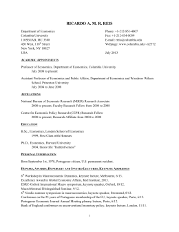
For example, the following chart from Stack Overflow Trends shows how the popularity of a single Python deep learning
library (PyTorch) has grown over the last few years.
Pytorch is just one of several Python libraries for deep learning and AI.
1.2.3 Features
Python is a high-level language, which means it is relatively easy to read, write and debug.
It has a relatively small core language that is easy to learn.
This core is supported by many libraries, which can be studied as required.
Python is flexible and pragmatic, supporting multiple programming styles (procedural, object-oriented, functional, etc.).
1.2. Introducing Python
7
Python Programming for Economics and Finance
1.2.4 Syntax and Design
One reason for Python’s popularity is its simple and elegant design.
To get a feeling for this, let’s look at an example.
The code below is written in Java rather than Python.
You do not need to read and understand this code!
import java.io.BufferedReader;
import java.io.FileReader;
import java.io.IOException;
public class CSVReader {
public static void main(String[] args) {
String filePath = "data.csv";
String line;
String splitBy = ",";
int columnIndex = 1;
double sum = 0;
int count = 0;
try (BufferedReader br = new BufferedReader(new FileReader(filePath))) {
while ((line = br.readLine()) != null) {
String[] values = line.split(splitBy);
if (values.length > columnIndex) {
try {
double value = Double.parseDouble(
values[columnIndex]
);
sum += value;
count++;
} catch (NumberFormatException e) {
System.out.println(
"Skipping non-numeric value: " +
values[columnIndex]
);
}
}
}
} catch (IOException e) {
e.printStackTrace();
}
if (count > 0) {
double average = sum / count;
System.out.println(
"Average of the second column: " + average
);
} else {
System.out.println(
"No valid numeric data found in the second column."
);
}
}
}
This Java code opens an imaginary file called data.csv and computes the mean of the values in the second column.
8
Chapter 1. About These Lectures
Python Programming for Economics and Finance
Here’s Python code that does the same thing.
Even if you don’t yet know Python, you can see that the code is far simpler and easier to read.
import csv
total, count = 0, 0
with open(data.csv, mode='r') as file:
reader = csv.reader(file)
for row in reader:
try:
total += float(row[1])
count += 1
except (ValueError, IndexError):
pass
print(f"Average: {total / count if count else 'No valid data'}")
1.2.5 The AI Connection
AI is in the process of taking over many tasks currently performed by humans, just as other forms of machinery have
done over the past few centuries.
Moreover, Python is playing a huge role in the advance of AI and machine learning.
This means that tech firms are pouring money into development of extremely powerful Python libraries.
Even if you don’t plan to work on AI and machine learning, you can benefit from learning to use some of these libraries
for your own projects in economics, finance and other fields of science.
These lectures will explain how.
1.3 Scientific Programming with Python
We have already discussed the importance of Python for AI, machine learning and data science
Python is also one of the dominant players in
• astronomy
• chemistry
• computational biology
• meteorology
• natural language processing
• etc.
Use of Python is also rising in economics, finance, and adjacent fields like operations research – which were previously
dominated by MATLAB / Excel / STATA / C / Fortran.
This section briefly showcases some examples of Python for general scientific programming.
1.3. Scientific Programming with Python
9
Python Programming for Economics and Finance
1.3.1 NumPy
One of the most important parts of scientific computing is working with data.
Data is often stored in matrices, vectors and arrays.
We can create a simple array of numbers with pure Python as follows:
a = [-3.14, 0, 3.14]
a
# A Python list
[-3.14, 0, 3.14]
This array is very small so it’s fine to work with pure Python.
But when we want to work with larger arrays in real programs we need more efficiency and more tools.
For this we need to use libraries for working with arrays.
For Python, the most important matrix and array processing library is NumPy library.
For example, let’s build a NumPy array with 100 elements
import numpy as np
# Load the library
a = np.linspace(-np.pi, np.pi, 100)
a
# Create even grid from -π to π
array([-3.14159265, -3.07812614, -3.01465962, -2.9511931 , -2.88772658,
-2.82426006, -2.76079354, -2.69732703, -2.63386051, -2.57039399,
-2.50692747, -2.44346095, -2.37999443, -2.31652792, -2.2530614 ,
-2.18959488, -2.12612836, -2.06266184, -1.99919533, -1.93572881,
-1.87226229, -1.80879577, -1.74532925, -1.68186273, -1.61839622,
-1.5549297 , -1.49146318, -1.42799666, -1.36453014, -1.30106362,
-1.23759711, -1.17413059, -1.11066407, -1.04719755, -0.98373103,
-0.92026451, -0.856798 , -0.79333148, -0.72986496, -0.66639844,
-0.60293192, -0.53946541, -0.47599889, -0.41253237, -0.34906585,
-0.28559933, -0.22213281, -0.1586663 , -0.09519978, -0.03173326,
0.03173326, 0.09519978, 0.1586663 , 0.22213281, 0.28559933,
0.34906585, 0.41253237, 0.47599889, 0.53946541, 0.60293192,
0.66639844, 0.72986496, 0.79333148, 0.856798 , 0.92026451,
0.98373103, 1.04719755, 1.11066407, 1.17413059, 1.23759711,
1.30106362, 1.36453014, 1.42799666, 1.49146318, 1.5549297 ,
1.61839622, 1.68186273, 1.74532925, 1.80879577, 1.87226229,
1.93572881, 1.99919533, 2.06266184, 2.12612836, 2.18959488,
2.2530614 , 2.31652792, 2.37999443, 2.44346095, 2.50692747,
2.57039399, 2.63386051, 2.69732703, 2.76079354, 2.82426006,
2.88772658, 2.9511931 , 3.01465962, 3.07812614, 3.14159265])
Now let’s transform this array by applying functions to it.
b = np.cos(a)
c = np.sin(a)
# Apply cosine to each element of a
# Apply sin to each element of a
Now we can easily take the inner product of b and c.
b @ c
10
Chapter 1. About These Lectures
Python Programming for Economics and Finance
np.float64(9.853229343548264e-16)
We can also do many other tasks, like
• compute the mean and variance of arrays
• build matrices and solve linear systems
• generate random arrays for simulation, etc.
We will discuss the details later in the lecture series, where we cover NumPy in depth.
1.3.2 NumPy Alternatives
While NumPy is still the king of array processing in Python, there are now important competitors.
Libraries such as JAX, Pytorch, and CuPy also have built in array types and array operations that can be very fast and
efficient.
In fact these libraries are better at exploiting parallelization and fast hardware, as we’ll explain later in this series.
However, you should still learn NumPy first because
• NumPy is simpler and provides a strong foundation, and
• libraries like JAX directly extend NumPy functionality and hence are easier to learn when you already know
NumPy.
This lecture series will provide you with extensive background in NumPy.
1.3.3 SciPy
The SciPy library is built on top of NumPy and provides additional functionality.
2
For example, let’s calculate ∫−2 𝜙(𝑧)𝑑𝑧 where 𝜙 is the standard normal density.
from scipy.stats import norm
from scipy.integrate import quad
ϕ = norm()
value, error = quad(ϕ.pdf, -2, 2)
value
# Integrate using Gaussian quadrature
0.9544997361036417
SciPy includes many of the standard routines used in
• linear algebra
• integration
• interpolation
• optimization
• distributions and statistical techniques
• signal processing
See them all here.
Later we’ll discuss SciPy in more detail.
1.3. Scientific Programming with Python
11
Python Programming for Economics and Finance
1.3.4 Graphics
A major strength of Python is data visualization.
The most popular and comprehensive Python library for creating figures and graphs is Matplotlib, with functionality
including
• plots, histograms, contour images, 3D graphs, bar charts etc.
• output in many formats (PDF, PNG, EPS, etc.)
• LaTeX integration
Example 2D plot with embedded LaTeX annotations
Example contour plot
Example 3D plot
More examples can be found in the Matplotlib thumbnail gallery.
Other graphics libraries include
• Plotly
• seaborn — a high-level interface for matplotlib
• Altair
• Bokeh
You can visit the Python Graph Gallery for more example plots drawn using a variety of libraries.
12
Chapter 1. About These Lectures
Python Programming for Economics and Finance
1.3. Scientific Programming with Python
13
Python Programming for Economics and Finance
14
Chapter 1. About These Lectures
Python Programming for Economics and Finance
1.3.5 Networks and Graphs
The study of networks is becoming an important part of scientific work in economics, finance and other fields.
For example, we are interesting in studying
• production networks
• networks of banks and financial institutions
• friendship and social networks
• etc.
Python has many libraries for studying networks and graphs.
One well-known example is NetworkX.
Its features include, among many other things:
• standard graph algorithms for analyzing networks
• plotting routines
Here’s some example code that generates and plots a random graph, with node color determined by the shortest path
length from a central node.
import networkx as nx
import matplotlib.pyplot as plt
np.random.seed(1234)
# Generate a random graph
p = dict((i, (np.random.uniform(0, 1), np.random.uniform(0, 1)))
for i in range(200))
g = nx.random_geometric_graph(200, 0.12, pos=p)
pos = nx.get_node_attributes(g, 'pos')
# Find node nearest the center point (0.5, 0.5)
dists = [(x - 0.5)**2 + (y - 0.5)**2 for x, y in list(pos.values())]
ncenter = np.argmin(dists)
# Plot graph, coloring by path length from central node
p = nx.single_source_shortest_path_length(g, ncenter)
plt.figure()
nx.draw_networkx_edges(g, pos, alpha=0.4)
nx.draw_networkx_nodes(g,
pos,
nodelist=list(p.keys()),
node_size=120, alpha=0.5,
node_color=list(p.values()),
cmap=plt.cm.jet_r)
plt.show()
1.3. Scientific Programming with Python
15
Python Programming for Economics and Finance
1.3.6 Other Scientific Libraries
As discussed above, there are literally thousands of scientific libraries for Python.
Some are small and do very specific tasks.
Others are huge in terms of lines of code and investment from coders and tech firms.
Here’s a short list of some important scientific libraries for Python not mentioned above.
• SymPy for symbolic algebra, including limits, derivatives and integrals
• statsmodels for statistical routines
• scikit-learn for machine learning
• Keras for machine learning
• Pyro and PyStan for Bayesian data analysis
• GeoPandas for spatial data analysis
• Dask for parallelization
• Numba for making Python run at the same speed as native machine code
• CVXPY for convex optimization
• scikit-image and OpenCV for processing and analyzing image data
• BeautifulSoup for extracting data from HTML and XML files
In this lecture series we will learn how to use many of these libraries for scientific computing tasks in economics and
finance.
16
Chapter 1. About These Lectures
CHAPTER
TWO
GETTING STARTED
2.1 Overview
In this lecture, you will learn how to
1. use Python in the cloud
2. get a local Python environment up and running
3. execute simple Python commands
4. run a sample program
5. install the code libraries that underpin these lectures
2.2 Python in the Cloud
The easiest way to get started coding in Python is by running it in the cloud.
(That is, by using a remote server that already has Python installed.)
One option that’s both free and reliable is Google Colab.
Colab also has the advantage of providing GPUs, which we will make use of in more advanced lectures.
Tutorials on how to get started with Google Colab can be found by web and video searches.
Most of our lectures include a “Launch notebook” button (with a play icon) on the top right connects you to an executable
version on Colab.
2.3 Local Install
Local installs are preferable if you have access to a suitable machine and plan to do a substantial amount of Python
programming.
At the same time, local installs require more work than a cloud option like Colab.
The rest of this lecture runs you through the some details associated with local installs.
17
Python Programming for Economics and Finance
2.3.1 The Anaconda Distribution
The core Python package is easy to install but not what you should choose for these lectures.
These lectures require the entire scientific programming ecosystem, which
• the core installation doesn’t provide
• is painful to install one piece at a time.
Hence the best approach for our purposes is to install a Python distribution that contains
1. the core Python language and
2. compatible versions of the most popular scientific libraries.
The best such distribution is Anaconda Python.
Anaconda is
• very popular
• cross-platform
• comprehensive
• completely unrelated to the Nicki Minaj song of the same name
Anaconda also comes with a package management system to organize your code libraries.
All of what follows assumes that you adopt this recommendation!
2.3.2 Installing Anaconda
To install Anaconda, download the binary and follow the instructions.
Important points:
• Make sure you install the correct version for your OS.
• If you are asked during the installation process whether you’d like to make Anaconda your default Python installation, say yes.
2.3.3 Updating conda
Anaconda supplies a tool called conda to manage and upgrade your Anaconda packages.
One conda command you should execute regularly is the one that updates the whole Anaconda distribution.
As a practice run, please execute the following
1. Open up a terminal
2. Type conda update conda
For more information on conda, type conda help in a terminal.
18
Chapter 2. Getting Started
Python Programming for Economics and Finance
2.4 Jupyter Notebooks
Jupyter notebooks are one of the many possible ways to interact with Python and the scientific libraries.
They use a browser-based interface to Python with
• The ability to write and execute Python commands.
• Formatted output in the browser, including tables, figures, animation, etc.
• The option to mix in formatted text and mathematical expressions.
Because of these features, Jupyter is now a major player in the scientific computing ecosystem.
Here’s an image showing execution of some code (borrowed from here) in a Jupyter notebook
While Jupyter isn’t the only way to code in Python, it’s great for when you wish to
• start coding in Python
• test new ideas or interact with small pieces of code
• use powerful online interactive environments such as Google Colab
• share or collaborate scientific ideas with students or colleagues
These lectures are designed for executing in Jupyter notebooks.
2.4.1 Starting the Jupyter Notebook
Once you have installed Anaconda, you can start the Jupyter notebook.
Either
• search for Jupyter in your applications menu, or
• open up a terminal and type jupyter notebook
– Windows users should substitute “Anaconda command prompt” for “terminal” in the previous line.
If you use the second option, you will see something like this
The output tells us the notebook is running at http://localhost:8888/
• localhost is the name of the local machine
• 8888 refers to port number 8888 on your computer
Thus, the Jupyter kernel is listening for Python commands on port 8888 of our local machine.
Hopefully, your default browser has also opened up with a web page that looks something like this
What you see here is called the Jupyter dashboard.
If you look at the URL at the top, it should be localhost:8888 or similar, matching the message above.
Assuming all this has worked OK, you can now click on New at the top right and select Python 3 or similar.
Here’s what shows up on our machine:
The notebook displays an active cell, into which you can type Python commands.
2.4. Jupyter Notebooks
19
Python Programming for Economics and Finance
20
Chapter 2. Getting Started
Python Programming for Economics and Finance
2.4.2 Notebook Basics
Let’s start with how to edit code and run simple programs.
Running Cells
Notice that, in the previous figure, the cell is surrounded by a green border.
This means that the cell is in edit mode.
In this mode, whatever you type will appear in the cell with the flashing cursor.
When you’re ready to execute the code in a cell, hit Shift-Enter instead of the usual Enter.
® Note
There are also menu and button options for running code in a cell that you can find by exploring.
Modal Editing
The next thing to understand about the Jupyter notebook is that it uses a modal editing system.
This means that the effect of typing at the keyboard depends on which mode you are in.
The two modes are
1. Edit mode
• Indicated by a green border around one cell, plus a blinking cursor
• Whatever you type appears as is in that cell
2.4. Jupyter Notebooks
21
Python Programming for Economics and Finance
22
Chapter 2. Getting Started
Python Programming for Economics and Finance
2.4. Jupyter Notebooks
23
Python Programming for Economics and Finance
24
Chapter 2. Getting Started
Python Programming for Economics and Finance
2. Command mode
• The green border is replaced by a blue border
• Keystrokes are interpreted as commands — for example, typing b adds a new cell below the current one
To switch to
• command mode from edit mode, hit the Esc key or Ctrl-M
• edit mode from command mode, hit Enter or click in a cell
The modal behavior of the Jupyter notebook is very efficient when you get used to it.
Inserting Unicode (e.g., Greek Letters)
Python supports unicode, allowing the use of characters such as 𝛼 and 𝛽 as names in your code.
In a code cell, try typing \alpha and then hitting the tab key on your keyboard.
A Test Program
Let’s run a test program.
Here’s an arbitrary program we can use: http://matplotlib.org/3.1.1/gallery/pie_and_polar_charts/polar_bar.html.
On that page, you’ll see the following code
import numpy as np
import matplotlib.pyplot as plt
# Fixing random state for reproducibility
np.random.seed(19680801)
# Compute pie slices
N = 20
θ = np.linspace(0.0, 2 * np.pi, N, endpoint=False)
radii = 10 * np.random.rand(N)
width = np.pi / 4 * np.random.rand(N)
colors = plt.cm.viridis(radii / 10.)
ax = plt.subplot(111, projection='polar')
ax.bar(θ, radii, width=width, bottom=0.0, color=colors, alpha=0.5)
plt.show()
2.4. Jupyter Notebooks
25
Python Programming for Economics and Finance
Don’t worry about the details for now — let’s just run it and see what happens.
The easiest way to run this code is to copy and paste it into a cell in the notebook.
Hopefully you will get a similar plot.
2.4.3 Working with the Notebook
Here are a few more tips on working with Jupyter notebooks.
Tab Completion
In the previous program, we executed the line import numpy as np
• NumPy is a numerical library we’ll work with in depth.
After this import command, functions in NumPy can be accessed with np.function_name type syntax.
• For example, try np.random.randn(3).
We can explore these attributes of np using the Tab key.
For example, here we type np.random.r and hit Tab
Jupyter offers several possible completions for you to choose from.
In this way, the Tab key helps remind you of what’s available and also saves you typing.
26
Chapter 2. Getting Started
Python Programming for Economics and Finance
2.4. Jupyter Notebooks
27
Python Programming for Economics and Finance
On-Line Help
To get help on np.random.randn, we can execute np.random.randn?.
Documentation appears in a split window of the browser, like so
Clicking on the top right of the lower split closes the on-line help.
We will learn more about how to create documentation like this later!
Other Content
In addition to executing code, the Jupyter notebook allows you to embed text, equations, figures and even videos in the
page.
For example, we can enter a mixture of plain text and LaTeX instead of code.
Next we Esc to enter command mode and then type m to indicate that we are writing Markdown, a mark-up language
similar to (but simpler than) LaTeX.
(You can also use your mouse to select Markdown from the Code drop-down box just below the list of menu items)
Now we Shift+Enter to produce this
2.4.4 Debugging Code
Debugging is the process of identifying and removing errors from a program.
You will spend a lot of time debugging code, so it is important to learn how to do it effectively.
If you are using a newer version of Jupyter, you should see a bug icon on the right end of the toolbar.
Clicking this icon will enable the Jupyter debugger.
® Note
You may also need to open the Debugger Panel (View -> Debugger Panel).
You can set breakpoints by clicking on the line number of the cell you want to debug.
When you run the cell, the debugger will stop at the breakpoint.
You can then step through the code line by line using the buttons on the “Next” button on the CALLSTACK toolbar
(located in the right hand window).
You can explore more functionality of the debugger in the Jupyter documentation.
2.4.5 Sharing Notebooks
Notebook files are just text files structured in JSON and typically ending with .ipynb.
You can share them in the usual way that you share files — or by using web services such as nbviewer.
The notebooks you see on that site are static html representations.
To run one, download it as an ipynb file by clicking on the download icon at the top right.
Save it somewhere, navigate to it from the Jupyter dashboard and then run as discussed above.
28
Chapter 2. Getting Started
Python Programming for Economics and Finance
2.4. Jupyter Notebooks
29
Python Programming for Economics and Finance
30
Chapter 2. Getting Started
Python Programming for Economics and Finance
2.4. Jupyter Notebooks
31
Python Programming for Economics and Finance
32
Chapter 2. Getting Started
Python Programming for Economics and Finance
® Note
If you are interested in sharing notebooks containing interactive content, you might want to check out Binder.
To collaborate with other people on notebooks, you might want to take a look at
• Google Colab
• Kaggle
To keep the code private and to use the familiar JupyterLab and Notebook interface, look into the JupyterLab RealTime Collaboration extension.
2.4.6 QuantEcon Notes
QuantEcon has its own site for sharing Jupyter notebooks related to economics – QuantEcon Notes.
Notebooks submitted to QuantEcon Notes can be shared with a link, and are open to comments and votes by the community.
2.5 Installing Libraries
Most of the libraries we need come in Anaconda.
Other libraries can be installed with pip or conda.
One library we’ll be using is QuantEcon.py.
You can install QuantEcon.py by starting Jupyter and typing
!conda install quantecon
into a cell.
Alternatively, you can type the following into a terminal
conda install quantecon
More instructions can be found on the library page.
To upgrade to the latest version, which you should do regularly, use
conda upgrade quantecon
Another library we will be using is interpolation.py.
This can be installed by typing in Jupyter
!conda install -c conda-forge interpolation
2.5. Installing Libraries
33
Python Programming for Economics and Finance
2.6 Working with Python Files
So far we’ve focused on executing Python code entered into a Jupyter notebook cell.
Traditionally most Python code has been run in a different way.
Code is first saved in a text file on a local machine
By convention, these text files have a .py extension.
We can create an example of such a file as follows:
%%writefile foo.py
print("foobar")
Writing foo.py
This writes the line print("foobar") into a file called foo.py in the local directory.
Here %%writefile is an example of a cell magic.
2.6.1 Editing and Execution
If you come across code saved in a *.py file, you’ll need to consider the following questions:
1. how should you execute it?
2. How should you modify or edit it?
Option 1: JupyterLab
JupyterLab is an integrated development environment built on top of Jupyter notebooks.
With JupyterLab you can edit and run *.py files as well as Jupyter notebooks.
To start JupyterLab, search for it in the applications menu or type jupyter-lab in a terminal.
Now you should be able to open, edit and run the file foo.py created above by opening it in JupyterLab.
Read the docs or search for a recent YouTube video to find more information.
Option 2: Using a Text Editor
One can also edit files using a text editor and then run them from within Jupyter notebooks.
A text editor is an application that is specifically designed to work with text files — such as Python programs.
Nothing beats the power and efficiency of a good text editor for working with program text.
A good text editor will provide
• efficient text editing commands (e.g., copy, paste, search and replace)
• syntax highlighting, etc.
34
Chapter 2. Getting Started
Python Programming for Economics and Finance
Right now, an extremely popular text editor for coding is VS Code.
VS Code is easy to use out of the box and has many high quality extensions.
Alternatively, if you want an outstanding free text editor and don’t mind a seemingly vertical learning curve plus long days
of pain and suffering while all your neural pathways are rewired, try Vim.
2.7 Exercises
® Exercise 2.7.1
If Jupyter is still running, quit by using Ctrl-C at the terminal where you started it.
Now launch again, but this time using jupyter notebook --no-browser.
This should start the kernel without launching the browser.
Note also the startup message: It should give you a URL such as http://localhost:8888 where the notebook
is running.
Now
1. Start your browser — or open a new tab if it’s already running.
2. Enter the URL from above (e.g. http://localhost:8888) in the address bar at the top.
You should now be able to run a standard Jupyter notebook session.
This is an alternative way to start the notebook that can also be handy.
This can also work when you accidentally close the webpage as long as the kernel is still running.
2.7. Exercises
35
Python Programming for Economics and Finance
36
Chapter 2. Getting Started
CHAPTER
THREE
AN INTRODUCTORY EXAMPLE
3.1 Overview
We’re now ready to start learning the Python language itself.
In this lecture, we will write and then pick apart small Python programs.
The objective is to introduce you to basic Python syntax and data structures.
Deeper concepts will be covered in later lectures.
You should have read the lecture on getting started with Python before beginning this one.
3.2 The Task: Plotting a White Noise Process
Suppose we want to simulate and plot the white noise process 𝜖0 , 𝜖1 , … , 𝜖𝑇 , where each draw 𝜖𝑡 is independent standard
normal.
In other words, we want to generate figures that look something like this:
(Here 𝑡 is on the horizontal axis and 𝜖𝑡 is on the vertical axis.)
We’ll do this in several different ways, each time learning something more about Python.
3.3 Version 1
Here are a few lines of code that perform the task we set
import numpy as np
import matplotlib.pyplot as plt
ϵ_values = np.random.randn(100)
plt.plot(ϵ_values)
plt.show()
37
Python Programming for Economics and Finance
Let’s break this program down and see how it works.
38
Chapter 3. An Introductory Example
Python Programming for Economics and Finance
3.3.1 Imports
The first two lines of the program import functionality from external code libraries.
The first line imports NumPy, a favorite Python package for tasks like
• working with arrays (vectors and matrices)
• common mathematical functions like cos and sqrt
• generating random numbers
• linear algebra, etc.
After import numpy as np we have access to these attributes via the syntax np.attribute.
Here’s two more examples
np.sqrt(4)
np.float64(2.0)
np.log(4)
np.float64(1.3862943611198906)
Why So Many Imports?
Python programs typically require multiple import statements.
The reason is that the core language is deliberately kept small, so that it’s easy to learn, maintain and improve.
When you want to do something interesting with Python, you almost always need to import additional functionality.
Packages
As stated above, NumPy is a Python package.
Packages are used by developers to organize code they wish to share.
In fact, a package is just a directory containing
1. files with Python code — called modules in Python speak
2. possibly some compiled code that can be accessed by Python (e.g., functions compiled from C or FORTRAN code)
3. a file called __init__.py that specifies what will be executed when we type import package_name
You can check the location of your __init__.py for NumPy in python by running the code:
import numpy as np
print(np.__file__)
3.3. Version 1
39
Python Programming for Economics and Finance
Subpackages
Consider the line ϵ_values = np.random.randn(100).
Here np refers to the package NumPy, while random is a subpackage of NumPy.
Subpackages are just packages that are subdirectories of another package.
For instance, you can find folder random under the directory of NumPy.
3.3.2 Importing Names Directly
Recall this code that we saw above
import numpy as np
np.sqrt(4)
np.float64(2.0)
Here’s another way to access NumPy’s square root function
from numpy import sqrt
sqrt(4)
np.float64(2.0)
This is also fine.
The advantage is less typing if we use sqrt often in our code.
The disadvantage is that, in a long program, these two lines might be separated by many other lines.
Then it’s harder for readers to know where sqrt came from, should they wish to.
3.3.3 Random Draws
Returning to our program that plots white noise, the remaining three lines after the import statements are
ϵ_values = np.random.randn(100)
plt.plot(ϵ_values)
plt.show()
40
Chapter 3. An Introductory Example
Python Programming for Economics and Finance
The first line generates 100 (quasi) independent standard normals and stores them in ϵ_values.
The next two lines genererate the plot.
We can and will look at various ways to configure and improve this plot below.
3.4 Alternative Implementations
Let’s try writing some alternative versions of our first program, which plotted IID draws from the standard normal distribution.
The programs below are less efficient than the original one, and hence somewhat artificial.
But they do help us illustrate some important Python syntax and semantics in a familiar setting.
3.4.1 A Version with a For Loop
Here’s a version that illustrates for loops and Python lists.
ts_length = 100
ϵ_values = []
# empty list
for i in range(ts_length):
e = np.random.randn()
ϵ_values.append(e)
plt.plot(ϵ_values)
plt.show()
3.4. Alternative Implementations
41
Python Programming for Economics and Finance
In brief,
• The first line sets the desired length of the time series.
• The next line creates an empty list called ϵ_values that will store the 𝜖𝑡 values as we generate them.
• The statement # empty list is a comment, and is ignored by Python’s interpreter.
• The next three lines are the for loop, which repeatedly draws a new random number 𝜖𝑡 and appends it to the end
of the list ϵ_values.
• The last two lines generate the plot and display it to the user.
Let’s study some parts of this program in more detail.
3.4.2 Lists
Consider the statement ϵ_values = [], which creates an empty list.
Lists are a native Python data structure used to group a collection of objects.
Items in lists are ordered, and duplicates are allowed in lists.
For example, try
x = [10, 'foo', False]
type(x)
list
The first element of x is an integer, the next is a string, and the third is a Boolean value.
When adding a value to a list, we can use the syntax list_name.append(some_value)
42
Chapter 3. An Introductory Example
Python Programming for Economics and Finance
x
[10, 'foo', False]
x.append(2.5)
x
[10, 'foo', False, 2.5]
Here append() is what’s called a method, which is a function “attached to” an object—in this case, the list x.
We’ll learn all about methods later on, but just to give you some idea,
• Python objects such as lists, strings, etc. all have methods that are used to manipulate data contained in the object.
• String objects have string methods, list objects have list methods, etc.
Another useful list method is pop()
x
[10, 'foo', False, 2.5]
x.pop()
2.5
x
[10, 'foo', False]
Lists in Python are zero-based (as in C, Java or Go), so the first element is referenced by x[0]
x[0]
# first element of x
10
x[1]
# second element of x
'foo'
3.4.3 The For Loop
Now let’s consider the for loop from the program above, which was
for i in range(ts_length):
e = np.random.randn()
ϵ_values.append(e)
Python executes the two indented lines ts_length times before moving on.
These two lines are called a code block, since they comprise the “block” of code that we are looping over.
Unlike most other languages, Python knows the extent of the code block only from indentation.
3.4. Alternative Implementations
43
Python Programming for Economics and Finance
In our program, indentation decreases after line ϵ_values.append(e), telling Python that this line marks the lower
limit of the code block.
More on indentation below—for now, let’s look at another example of a for loop
animals = ['dog', 'cat', 'bird']
for animal in animals:
print("The plural of " + animal + " is " + animal + "s")
The plural of dog is dogs
The plural of cat is cats
The plural of bird is birds
This example helps to clarify how the for loop works: When we execute a loop of the form
for variable_name in sequence:
<code block>
The Python interpreter performs the following:
• For each element of the sequence, it “binds” the name variable_name to that element and then executes
the code block.
3.4.4 A Comment on Indentation
In discussing the for loop, we explained that the code blocks being looped over are delimited by indentation.
In fact, in Python, all code blocks (i.e., those occurring inside loops, if clauses, function definitions, etc.) are delimited
by indentation.
Thus, unlike most other languages, whitespace in Python code affects the output of the program.
Once you get used to it, this is a good thing: It
• forces clean, consistent indentation, improving readability
• removes clutter, such as the brackets or end statements used in other languages
On the other hand, it takes a bit of care to get right, so please remember:
• The line before the start of a code block always ends in a colon
– for i in range(10):
– if x > y:
– while x < 100:
– etc.
• All lines in a code block must have the same amount of indentation.
• The Python standard is 4 spaces, and that’s what you should use.
44
Chapter 3. An Introductory Example
Python Programming for Economics and Finance
3.4.5 While Loops
The for loop is the most common technique for iteration in Python.
But, for the purpose of illustration, let’s modify the program above to use a while loop instead.
ts_length = 100
ϵ_values = []
i = 0
while i < ts_length:
e = np.random.randn()
ϵ_values.append(e)
i = i + 1
plt.plot(ϵ_values)
plt.show()
A while loop will keep executing the code block delimited by indentation until the condition (i < ts_length) is
satisfied.
In this case, the program will keep adding values to the list ϵ_values until i equals ts_length:
i == ts_length #the ending condition for the while loop
True
Note that
• the code block for the while loop is again delimited only by indentation.
• the statement i = i + 1 can be replaced by i += 1.
3.4. Alternative Implementations
45
Python Programming for Economics and Finance
3.5 Another Application
Let’s do one more application before we turn to exercises.
In this application, we plot the balance of a bank account over time.
There are no withdraws over the time period, the last date of which is denoted by 𝑇 .
The initial balance is 𝑏0 and the interest rate is 𝑟.
The balance updates from period 𝑡 to 𝑡 + 1 according to 𝑏𝑡+1 = (1 + 𝑟)𝑏𝑡 .
In the code below, we generate and plot the sequence 𝑏0 , 𝑏1 , … , 𝑏𝑇 .
Instead of using a Python list to store this sequence, we will use a NumPy array.
r = 0.025
# interest rate
T = 50
# end date
b = np.empty(T+1) # an empty NumPy array, to store all b_t
b[0] = 10
# initial balance
for t in range(T):
b[t+1] = (1 + r) * b[t]
plt.plot(b, label='bank balance')
plt.legend()
plt.show()
The statement b = np.empty(T+1) allocates storage in memory for T+1 (floating point) numbers.
These numbers are filled in by the for loop.
46
Chapter 3. An Introductory Example
Python Programming for Economics and Finance
Allocating memory at the start is more efficient than using a Python list and append, since the latter must repeatedly
ask for storage space from the operating system.
Notice that we added a legend to the plot — a feature you will be asked to use in the exercises.
3.6 Exercises
Now we turn to exercises. It is important that you complete them before continuing, since they present new concepts we
will need.
® Exercise 3.6.1
Your first task is to simulate and plot the correlated time series
𝑥𝑡+1 = 𝛼 𝑥𝑡 + 𝜖𝑡+1
where
𝑥0 = 0
and
𝑡 = 0, … , 𝑇
The sequence of shocks {𝜖𝑡 } is assumed to be IID and standard normal.
In your solution, restrict your import statements to
import numpy as np
import matplotlib.pyplot as plt
Set 𝑇 = 200 and 𝛼 = 0.9.
® Solution to Exercise 3.6.1
Here’s one solution.
α = 0.9
T = 200
x = np.empty(T+1)
x[0] = 0
for t in range(T):
x[t+1] = α * x[t] + np.random.randn()
plt.plot(x)
plt.show()
3.6. Exercises
47
Python Programming for Economics and Finance
® Exercise 3.6.2
Starting with your solution to exercise 1, plot three simulated time series, one for each of the cases 𝛼 = 0, 𝛼 = 0.8
and 𝛼 = 0.98.
Use a for loop to step through the 𝛼 values.
If you can, add a legend, to help distinguish between the three time series.
b Hint
• If you call the plot() function multiple times before calling show(), all of the lines you produce will
end up on the same figure.
• For the legend, noted that suppose var = 42, the expression f'foo{var}' evaluates to 'foo42'.
® Solution to Exercise 3.6.2
α_values = [0.0, 0.8, 0.98]
T = 200
x = np.empty(T+1)
for α in α_values:
x[0] = 0
for t in range(T):
x[t+1] = α * x[t] + np.random.randn()
48
Chapter 3. An Introductory Example
Python Programming for Economics and Finance
plt.plot(x, label=f'$\\alpha = {α}$')
plt.legend()
plt.show()
® Note
f'$\\alpha = {α}$' in the solution is an application of f-String, which allows you to use {} to contain an
expression.
The contained expression will be evaluated, and the result will be placed into the string.
® Exercise 3.6.3
Similar to the previous exercises, plot the time series
𝑥𝑡+1 = 𝛼 |𝑥𝑡 | + 𝜖𝑡+1
where 𝑥0 = 0
and 𝑡 = 0, … , 𝑇
Use 𝑇 = 200, 𝛼 = 0.9 and {𝜖𝑡 } as before.
Search online for a function that can be used to compute the absolute value |𝑥𝑡 |.
® Solution to Exercise 3.6.3
Here’s one solution:
3.6. Exercises
49
Python Programming for Economics and Finance
α = 0.9
T = 200
x = np.empty(T+1)
x[0] = 0
for t in range(T):
x[t+1] = α * np.abs(x[t]) + np.random.randn()
plt.plot(x)
plt.show()
® Exercise 3.6.4
One important aspect of essentially all programming languages is branching and conditions.
In Python, conditions are usually implemented with if–else syntax.
Here’s an example, that prints -1 for each negative number in an array and 1 for each nonnegative number
numbers = [-9, 2.3, -11, 0]
for x in numbers:
if x < 0:
print(-1)
else:
print(1)
-1
1
-1
1
50
Chapter 3. An Introductory Example
Python Programming for Economics and Finance
Now, write a new solution to Exercise 3 that does not use an existing function to compute the absolute value.
Replace this existing function with an if–else condition.
® Solution to Exercise 3.6.4
Here’s one way:
α = 0.9
T = 200
x = np.empty(T+1)
x[0] = 0
for t in range(T):
if x[t] < 0:
abs_x = - x[t]
else:
abs_x = x[t]
x[t+1] = α * abs_x + np.random.randn()
plt.plot(x)
plt.show()
Here’s a shorter way to write the same thing:
3.6. Exercises
51
Python Programming for Economics and Finance
α = 0.9
T = 200
x = np.empty(T+1)
x[0] = 0
for t in range(T):
abs_x = - x[t] if x[t] < 0 else x[t]
x[t+1] = α * abs_x + np.random.randn()
plt.plot(x)
plt.show()
® Exercise 3.6.5
Here’s a harder exercise, that takes some thought and planning.
The task is to compute an approximation to 𝜋 using Monte Carlo.
Use no imports besides
import numpy as np
52
Chapter 3. An Introductory Example
Python Programming for Economics and Finance
b Hint
Your hints are as follows:
• If 𝑈 is a bivariate uniform random variable on the unit square (0, 1)2 , then the probability that 𝑈 lies in a
subset 𝐵 of (0, 1)2 is equal to the area of 𝐵.
• If 𝑈1 , … , 𝑈𝑛 are IID copies of 𝑈 , then, as 𝑛 gets large, the fraction that falls in 𝐵, converges to the
probability of landing in 𝐵.
• For a circle, 𝑎𝑟𝑒𝑎 = 𝜋 ∗ 𝑟𝑎𝑑𝑖𝑢𝑠2 .
® Solution to Exercise 3.6.5
Consider the circle of diameter 1 embedded in the unit square.
Let 𝐴 be its area and let 𝑟 = 1/2 be its radius.
If we know 𝜋 then we can compute 𝐴 via 𝐴 = 𝜋𝑟2 .
But here the point is to compute 𝜋, which we can do by 𝜋 = 𝐴/𝑟2 .
Summary: If we can estimate the area of a circle with diameter 1, then dividing by 𝑟2 = (1/2)2 = 1/4 gives an
estimate of 𝜋.
We estimate the area by sampling bivariate uniforms and looking at the fraction that falls into the circle.
n = 1000000 # sample size for Monte Carlo simulation
count = 0
for i in range(n):
# drawing random positions on the square
u, v = np.random.uniform(), np.random.uniform()
# check whether the point falls within the boundary
# of the unit circle centred at (0.5,0.5)
d = np.sqrt((u - 0.5)**2 + (v - 0.5)**2)
# if it falls within the inscribed circle,
# add it to the count
if d < 0.5:
count += 1
area_estimate = count / n
print(area_estimate * 4)
# dividing by radius**2
3.144768
3.6. Exercises
53
Python Programming for Economics and Finance
54
Chapter 3. An Introductory Example
CHAPTER
FOUR
FUNCTIONS
4.1 Overview
Functions are an extremely useful construct provided by almost all programming.
We have already met several functions, such as
• the sqrt() function from NumPy and
• the built-in print() function
In this lecture we’ll
1. treat functions systematically and cover syntax and use-cases, and
2. learn to do is build our own user-defined functions.
We will use the following imports.
import numpy as np
import matplotlib.pyplot as plt
4.2 Function Basics
A function is a named section of a program that implements a specific task.
Many functions exist already and we can use them as is.
First we review these functions and then discuss how we can build our own.
4.2.1 Built-In Functions
Python has a number of built-in functions that are available without import.
We have already met some
max(19, 20)
20
print('foobar')
55
Python Programming for Economics and Finance
foobar
str(22)
'22'
type(22)
int
The full list of Python built-ins is here.
4.2.2 Third Party Functions
If the built-in functions don’t cover what we need, we either need to import functions or create our own.
Examples of importing and using functions were given in the previous lecture
Here’s another one, which tests whether a given year is a leap year:
import calendar
calendar.isleap(2024)
True
4.3 Defining Functions
In many instances it’s useful to be able to define our own functions.
Let’s start by discussing how it’s done.
4.3.1 Basic Syntax
Here’s a very simple Python function, that implements the mathematical function 𝑓(𝑥) = 2𝑥 + 1
def f(x):
return 2 * x + 1
Now that we’ve defined this function, let’s call it and check whether it does what we expect:
f(1)
3
f(10)
21
Here’s a longer function, that computes the absolute value of a given number.
(Such a function already exists as a built-in, but let’s write our own for the exercise.)
56
Chapter 4. Functions
Python Programming for Economics and Finance
def new_abs_function(x):
if x < 0:
abs_value = -x
else:
abs_value = x
return abs_value
Let’s review the syntax here.
• def is a Python keyword used to start function definitions.
• def new_abs_function(x): indicates that the function is called new_abs_function and that it has a
single argument x.
• The indented code is a code block called the function body.
• The return keyword indicates that abs_value is the object that should be returned to the calling code.
This whole function definition is read by the Python interpreter and stored in memory.
Let’s call it to check that it works:
print(new_abs_function(3))
print(new_abs_function(-3))
3
3
Note that a function can have arbitrarily many return statements (including zero).
Execution of the function terminates when the first return is hit, allowing code like the following example
def f(x):
if x < 0:
return 'negative'
return 'nonnegative'
(Writing functions with multiple return statements is typically discouraged, as it can make logic hard to follow.)
Functions without a return statement automatically return the special Python object None.
4.3.2 Keyword Arguments
In a previous lecture, you came across the statement
plt.plot(x, 'b-', label="white noise")
In this call to Matplotlib’s plot function, notice that the last argument is passed in name=argument syntax.
This is called a keyword argument, with label being the keyword.
Non-keyword arguments are called positional arguments, since their meaning is determined by order
• plot(x, 'b-') differs from plot('b-', x)
Keyword arguments are particularly useful when a function has a lot of arguments, in which case it’s hard to remember
the right order.
You can adopt keyword arguments in user-defined functions with no difficulty.
The next example illustrates the syntax
4.3. Defining Functions
57
Python Programming for Economics and Finance
def f(x, a=1, b=1):
return a + b * x
The keyword argument values we supplied in the definition of f become the default values
f(2)
3
They can be modified as follows
f(2, a=4, b=5)
14
4.3.3 The Flexibility of Python Functions
As we discussed in the previous lecture, Python functions are very flexible.
In particular
• Any number of functions can be defined in a given file.
• Functions can be (and often are) defined inside other functions.
• Any object can be passed to a function as an argument, including other functions.
• A function can return any kind of object, including functions.
We will give examples of how straightforward it is to pass a function to a function in the following sections.
4.3.4 One-Line Functions: lambda
The lambda keyword is used to create simple functions on one line.
For example, the definitions
def f(x):
return x**3
and
f = lambda x: x**3
are entirely equivalent.
2
To see why lambda is useful, suppose that we want to calculate ∫0 𝑥3 𝑑𝑥 (and have forgotten our high-school calculus).
The SciPy library has a function called quad that will do this calculation for us.
The syntax of the quad function is quad(f, a, b) where f is a function and a and b are numbers.
To create the function 𝑓(𝑥) = 𝑥3 we can use lambda as follows
from scipy.integrate import quad
quad(lambda x: x**3, 0, 2)
58
Chapter 4. Functions
Python Programming for Economics and Finance
(4.0, 4.440892098500626e-14)
Here the function created by lambda is said to be anonymous because it was never given a name.
4.3.5 Why Write Functions?
User-defined functions are important for improving the clarity of your code by
• separating different strands of logic
• facilitating code reuse
(Writing the same thing twice is almost always a bad idea)
We will say more about this later.
4.4 Applications
4.4.1 Random Draws
Consider again this code from the previous lecture
ts_length = 100
ϵ_values = []
# empty list
for i in range(ts_length):
e = np.random.randn()
ϵ_values.append(e)
plt.plot(ϵ_values)
plt.show()
4.4. Applications
59
Python Programming for Economics and Finance
We will break this program into two parts:
1. A user-defined function that generates a list of random variables.
2. The main part of the program that
1. calls this function to get data
2. plots the data
This is accomplished in the next program
def generate_data(n):
ϵ_values = []
for i in range(n):
e = np.random.randn()
ϵ_values.append(e)
return ϵ_values
data = generate_data(100)
plt.plot(data)
plt.show()
60
Chapter 4. Functions
Python Programming for Economics and Finance
When the interpreter gets to the expression generate_data(100), it executes the function body with n set equal to
100.
The net result is that the name data is bound to the list ϵ_values returned by the function.
4.4.2 Adding Conditions
Our function generate_data() is rather limited.
Let’s make it slightly more useful by giving it the ability to return either standard normals or uniform random variables
on (0, 1) as required.
This is achieved in the next piece of code.
def generate_data(n, generator_type):
ϵ_values = []
for i in range(n):
if generator_type == 'U':
e = np.random.uniform(0, 1)
else:
e = np.random.randn()
ϵ_values.append(e)
return ϵ_values
data = generate_data(100, 'U')
plt.plot(data)
plt.show()
4.4. Applications
61
Python Programming for Economics and Finance
Hopefully, the syntax of the if/else clause is self-explanatory, with indentation again delimiting the extent of the code
blocks.
Notes
• We are passing the argument U as a string, which is why we write it as 'U'.
• Notice that equality is tested with the == syntax, not =.
– For example, the statement a = 10 assigns the name a to the value 10.
– The expression a == 10 evaluates to either True or False, depending on the value of a.
Now, there are several ways that we can simplify the code above.
For example, we can get rid of the conditionals all together by just passing the desired generator type as a function.
To understand this, consider the following version.
def generate_data(n, generator_type):
ϵ_values = []
for i in range(n):
e = generator_type()
ϵ_values.append(e)
return ϵ_values
data = generate_data(100, np.random.uniform)
plt.plot(data)
plt.show()
62
Chapter 4. Functions
Python Programming for Economics and Finance
Now, when we call the function generate_data(), we pass np.random.uniform as the second argument.
This object is a function.
When the function call generate_data(100, np.random.uniform) is executed, Python runs the function
code block with n equal to 100 and the name generator_type “bound” to the function np.random.uniform.
• While these lines are executed, the names generator_type and np.random.uniform are “synonyms”,
and can be used in identical ways.
This principle works more generally—for example, consider the following piece of code
max(7, 2, 4)
# max() is a built-in Python function
7
m = max
m(7, 2, 4)
7
Here we created another name for the built-in function max(), which could then be used in identical ways.
In the context of our program, the ability to bind new names to functions means that there is no problem passing a function
as an argument to another function—as we did above.
4.4. Applications
63
Python Programming for Economics and Finance
4.5 Recursive Function Calls (Advanced)
This is an advanced topic that you should feel free to skip.
At the same time, it’s a neat idea that you should learn it at some stage of your programming career.
Basically, a recursive function is a function that calls itself.
For example, consider the problem of computing 𝑥𝑡 for some t when
𝑥𝑡+1 = 2𝑥𝑡 ,
𝑥0 = 1
(4.1)
Obviously the answer is 2𝑡 .
We can compute this easily enough with a loop
def x_loop(t):
x = 1
for i in range(t):
x = 2 * x
return x
We can also use a recursive solution, as follows
def x(t):
if t == 0:
return 1
else:
return 2 * x(t-1)
What happens here is that each successive call uses it’s own frame in the stack
• a frame is where the local variables of a given function call are held
• stack is memory used to process function calls
– a First In Last Out (FILO) queue
This example is somewhat contrived, since the first (iterative) solution would usually be preferred to the recursive solution.
We’ll meet less contrived applications of recursion later on.
4.6 Exercises
® Exercise 4.6.1
Recall that 𝑛! is read as “𝑛 factorial” and defined as 𝑛! = 𝑛 × (𝑛 − 1) × ⋯ × 2 × 1.
We will only consider 𝑛 as a positive integer here.
There are functions to compute this in various modules, but let’s write our own version as an exercise.
In particular, write a function factorial such that factorial(n) returns 𝑛! for any positive integer 𝑛.
64
Chapter 4. Functions
Python Programming for Economics and Finance
® Solution to Exercise 4.6.1
Here’s one solution:
def factorial(n):
k = 1
for i in range(n):
k = k * (i + 1)
return k
factorial(4)
24
® Exercise 4.6.2
The binomial random variable 𝑌 ∼ 𝐵𝑖𝑛(𝑛, 𝑝) represents the number of successes in 𝑛 binary trials, where each trial
succeeds with probability 𝑝.
Without any import besides from numpy.random import uniform, write a function binomial_rv such
that binomial_rv(n, p) generates one draw of 𝑌 .
b Hint
If 𝑈 is uniform on (0, 1) and 𝑝 ∈ (0, 1), then the expression U < p evaluates to True with probability 𝑝.
® Solution to Exercise 4.6.2
Here is one solution:
from numpy.random import uniform
def binomial_rv(n, p):
count = 0
for i in range(n):
U = uniform()
if U < p:
count = count + 1
return count
# Or count += 1
binomial_rv(10, 0.5)
7
® Exercise 4.6.3
First, write a function that returns one realization of the following random device
1. Flip an unbiased coin 10 times.
2. If a head occurs k or more times consecutively within this sequence at least once, pay one dollar.
3. If not, pay nothing.
4.6. Exercises
65
Python Programming for Economics and Finance
Second, write another function that does the same task except that the second rule of the above random device
becomes
• If a head occurs k or more times within this sequence, pay one dollar.
Use no import besides from numpy.random import uniform.
® Solution to Exercise 4.6.3
Here’s a function for the first random device.
from numpy.random import uniform
def draw(k):
# pays if k consecutive successes in a sequence
payoff = 0
count = 0
for i in range(10):
U = uniform()
count = count + 1 if U < 0.5 else 0
print(count)
# print counts for clarity
if count == k:
payoff = 1
return payoff
draw(3)
0
0
1
0
0
0
1
2
0
1
0
Here’s another function for the second random device.
def draw_new(k):
# pays if k successes in a sequence
payoff = 0
count = 0
for i in range(10):
U = uniform()
count = count + ( 1 if U < 0.5 else 0 )
print(count)
if count == k:
payoff = 1
return payoff
draw_new(3)
66
Chapter 4. Functions
Python Programming for Economics and Finance
0
1
1
1
1
1
2
2
2
3
1
4.7 Advanced Exercises
In the following exercises, we will write recursive functions together.
® Exercise 4.7.1
The Fibonacci numbers are defined by
𝑥𝑡+1 = 𝑥𝑡 + 𝑥𝑡−1 ,
𝑥0 = 0, 𝑥1 = 1
(4.2)
The first few numbers in the sequence are 0, 1, 1, 2, 3, 5, 8, 13, 21, 34, 55.
Write a function to recursively compute the 𝑡-th Fibonacci number for any 𝑡.
® Solution to Exercise 4.7.1
Here’s the standard solution
def x(t):
if t == 0:
return 0
if t == 1:
return 1
else:
return x(t-1) + x(t-2)
Let’s test it
print([x(i) for i in range(10)])
[0, 1, 1, 2, 3, 5, 8, 13, 21, 34]
® Exercise 4.7.2
Rewrite the function factorial() in from Exercise 1 using recursion.
4.7. Advanced Exercises
67
Python Programming for Economics and Finance
® Solution to Exercise 4.7.2
Here’s the standard solution
def recursion_factorial(n):
if n == 1:
return n
else:
return n * recursion_factorial(n-1)
Let’s test it
print([recursion_factorial(i) for i in range(1, 10)])
[1, 2, 6, 24, 120, 720, 5040, 40320, 362880]
68
Chapter 4. Functions
CHAPTER
FIVE
PYTHON ESSENTIALS
5.1 Overview
We have covered a lot of material quite quickly, with a focus on examples.
Now let’s cover some core features of Python in a more systematic way.
This approach is less exciting but helps clear up some details.
5.2 Data Types
Computer programs typically keep track of a range of data types.
For example, 1.5 is a floating point number, while 1 is an integer.
Programs need to distinguish between these two types for various reasons.
One is that they are stored in memory differently.
Another is that arithmetic operations are different
• For example, floating point arithmetic is implemented on most machines by a specialized Floating Point Unit
(FPU).
In general, floats are more informative but arithmetic operations on integers are faster and more accurate.
Python provides numerous other built-in Python data types, some of which we’ve already met
• strings, lists, etc.
Let’s learn a bit more about them.
5.2.1 Primitive Data Types
Boolean Values
One simple data type is Boolean values, which can be either True or False
x = True
x
True
We can check the type of any object in memory using the type() function.
69
Python Programming for Economics and Finance
type(x)
bool
In the next line of code, the interpreter evaluates the expression on the right of = and binds y to this value
y = 100 < 10
y
False
type(y)
bool
In arithmetic expressions, True is converted to 1 and False is converted 0.
This is called Boolean arithmetic and is often useful in programming.
Here are some examples
x + y
1
x * y
0
True + True
2
bools = [True, True, False, True]
# List of Boolean values
sum(bools)
3
Numeric Types
Numeric types are also important primitive data types.
We have seen integer and float types before.
Complex numbers are another primitive data type in Python
x = complex(1, 2)
y = complex(2, 1)
print(x * y)
type(x)
70
Chapter 5. Python Essentials
Python Programming for Economics and Finance
5j
complex
5.2.2 Containers
Python has several basic types for storing collections of (possibly heterogeneous) data.
We’ve already discussed lists.
A related data type is tuples, which are “immutable” lists
x = ('a', 'b')
x = 'a', 'b'
x
# Parentheses instead of the square brackets
# Or no brackets --- the meaning is identical
('a', 'b')
type(x)
tuple
In Python, an object is called immutable if, once created, the object cannot be changed.
Conversely, an object is mutable if it can still be altered after creation.
Python lists are mutable
x = [1, 2]
x[0] = 10
x
[10, 2]
But tuples are not
x = (1, 2)
x[0] = 10
--------------------------------------------------------------------------TypeError
Traceback (most recent call last)
Cell In[13], line 2
1 x = (1, 2)
----> 2 x[0] = 10
TypeError: 'tuple' object does not support item assignment
We’ll say more about the role of mutable and immutable data a bit later.
Tuples (and lists) can be “unpacked” as follows
integers = (10, 20, 30)
x, y, z = integers
x
5.2. Data Types
71
Python Programming for Economics and Finance
10
y
20
You’ve actually seen an example of this already.
Tuple unpacking is convenient and we’ll use it often.
Slice Notation
To access multiple elements of a sequence (a list, a tuple or a string), you can use Python’s slice notation.
For example,
a = ["a", "b", "c", "d", "e"]
a[1:]
['b', 'c', 'd', 'e']
a[1:3]
['b', 'c']
The general rule is that a[m:n] returns n - m elements, starting at a[m].
Negative numbers are also permissible
a[-2:]
# Last two elements of the list
['d', 'e']
You can also use the format [start:end:step] to specify the step
a[::2]
['a', 'c', 'e']
Using a negative step, you can return the sequence in a reversed order
a[-2::-1] # Walk backwards from the second last element to the first element
['d', 'c', 'b', 'a']
The same slice notation works on tuples and strings
s = 'foobar'
s[-3:] # Select the last three elements
'bar'
72
Chapter 5. Python Essentials
Python Programming for Economics and Finance
Sets and Dictionaries
Two other container types we should mention before moving on are sets and dictionaries.
Dictionaries are much like lists, except that the items are named instead of numbered
d = {'name': 'Frodo', 'age': 33}
type(d)
dict
d['age']
33
The names 'name' and 'age' are called the keys.
The objects that the keys are mapped to ('Frodo' and 33) are called the values.
Sets are unordered collections without duplicates, and set methods provide the usual set-theoretic operations
s1 = {'a', 'b'}
type(s1)
set
s2 = {'b', 'c'}
s1.issubset(s2)
False
s1.intersection(s2)
{'b'}
The set() function creates sets from sequences
s3 = set(('foo', 'bar', 'foo'))
s3
{'bar', 'foo'}
5.3 Input and Output
Let’s briefly review reading and writing to text files, starting with writing
f = open('newfile.txt', 'w')
f.write('Testing\n')
f.write('Testing again')
f.close()
# Open 'newfile.txt' for writing
# Here '\n' means new line
Here
5.3. Input and Output
73
Python Programming for Economics and Finance
• The built-in function open() creates a file object for writing to.
• Both write() and close() are methods of file objects.
Where is this file that we’ve created?
Recall that Python maintains a concept of the present working directory (pwd) that can be located from with Jupyter or
IPython via
%pwd
'/home/runner/work/lecture-python-programming.myst/lecture-python-programming.myst/
↪lectures'
If a path is not specified, then this is where Python writes to.
We can also use Python to read the contents of newline.txt as follows
f = open('newfile.txt', 'r')
out = f.read()
out
'Testing\nTesting again'
print(out)
Testing
Testing again
In fact, the recommended approach in modern Python is to use a with statement to ensure the files are properly acquired
and released.
Containing the operations within the same block also improves the clarity of your code.
® Note
This kind of block is formally referred to as a context.
Let’s try to convert the two examples above into a with statement.
We change the writing example first
with open('newfile.txt', 'w') as f:
f.write('Testing\n')
f.write('Testing again')
Note that we do not need to call the close() method since the with block will ensure the stream is closed at the end
of the block.
With slight modifications, we can also read files using with
with open('newfile.txt', 'r') as fo:
out = fo.read()
print(out)
Testing
Testing again
74
Chapter 5. Python Essentials
Python Programming for Economics and Finance
Now suppose that we want to read input from one file and write output to another. Here’s how we could accomplish this
task while correctly acquiring and returning resources to the operating system using with statements:
with open("newfile.txt", "r") as f:
file = f.readlines()
with open("output.txt", "w") as fo:
for i, line in enumerate(file):
fo.write(f'Line {i}: {line} \n')
The output file will be
with open('output.txt', 'r') as fo:
print(fo.read())
Line 0: Testing
Line 1: Testing again
We can simplify the example above by grouping the two with statements into one line
with open("newfile.txt", "r") as f, open("output2.txt", "w") as fo:
for i, line in enumerate(f):
fo.write(f'Line {i}: {line} \n')
The output file will be the same
with open('output2.txt', 'r') as fo:
print(fo.read())
Line 0: Testing
Line 1: Testing again
Suppose we want to continue to write into the existing file instead of overwriting it.
we can switch the mode to a which stands for append mode
with open('output2.txt', 'a') as fo:
fo.write('\nThis is the end of the file')
with open('output2.txt', 'r') as fo:
print(fo.read())
Line 0: Testing
Line 1: Testing again
This is the end of the file
® Note
Note that we only covered r, w, and a mode here, which are the most commonly used modes. Python provides a
variety of modes that you could experiment with.
5.3. Input and Output
75
Python Programming for Economics and Finance
5.3.1 Paths
Note that if newfile.txt is not in the present working directory then this call to open() fails.
In this case, you can shift the file to the pwd or specify the full path to the file
f = open('insert_full_path_to_file/newfile.txt', 'r')
5.4 Iterating
One of the most important tasks in computing is stepping through a sequence of data and performing a given action.
One of Python’s strengths is its simple, flexible interface to this kind of iteration via the for loop.
5.4.1 Looping over Different Objects
Many Python objects are “iterable”, in the sense that they can be looped over.
To give an example, let’s write the file us_cities.txt, which lists US cities and their population, to the present working
directory.
%%writefile us_cities.txt
new york: 8244910
los angeles: 3819702
chicago: 2707120
houston: 2145146
philadelphia: 1536471
phoenix: 1469471
san antonio: 1359758
san diego: 1326179
dallas: 1223229
Overwriting us_cities.txt
Here %%writefile is an IPython cell magic.
Suppose that we want to make the information more readable, by capitalizing names and adding commas to mark thousands.
The program below reads the data in and makes the conversion:
data_file = open('us_cities.txt', 'r')
for line in data_file:
city, population = line.split(':')
city = city.title()
population = f'{int(population):,}'
print(city.ljust(15) + population)
data_file.close()
New York
Los Angeles
Chicago
Houston
Philadelphia
# Tuple unpacking
# Capitalize city names
# Add commas to numbers
8,244,910
3,819,702
2,707,120
2,145,146
1,536,471
(continues on next page)
76
Chapter 5. Python Essentials
Python Programming for Economics and Finance
(continued from previous page)
Phoenix
San Antonio
San Diego
Dallas
1,469,471
1,359,758
1,326,179
1,223,229
Here f' is an f-string used for inserting variables into strings.
The reformatting of each line is the result of three different string methods, the details of which can be left till later.
The interesting part of this program for us is line 2, which shows that
1. The file object data_file is iterable, in the sense that it can be placed to the right of in within a for loop.
2. Iteration steps through each line in the file.
This leads to the clean, convenient syntax shown in our program.
Many other kinds of objects are iterable, and we’ll discuss some of them later on.
5.4.2 Looping without Indices
One thing you might have noticed is that Python tends to favor looping without explicit indexing.
For example,
x_values = [1, 2, 3]
for x in x_values:
print(x * x)
# Some iterable x
1
4
9
is preferred to
for i in range(len(x_values)):
print(x_values[i] * x_values[i])
1
4
9
When you compare these two alternatives, you can see why the first one is preferred.
Python provides some facilities to simplify looping without indices.
One is zip(), which is used for stepping through pairs from two sequences.
For example, try running the following code
countries = ('Japan', 'Korea', 'China')
cities = ('Tokyo', 'Seoul', 'Beijing')
for country, city in zip(countries, cities):
print(f'The capital of {country} is {city}')
The capital of Japan is Tokyo
The capital of Korea is Seoul
The capital of China is Beijing
5.4. Iterating
77
Python Programming for Economics and Finance
The zip() function is also useful for creating dictionaries — for example
names = ['Tom', 'John']
marks = ['E', 'F']
dict(zip(names, marks))
{'Tom': 'E', 'John': 'F'}
If we actually need the index from a list, one option is to use enumerate().
To understand what enumerate() does, consider the following example
letter_list = ['a', 'b', 'c']
for index, letter in enumerate(letter_list):
print(f"letter_list[{index}] = '{letter}'")
letter_list[0] = 'a'
letter_list[1] = 'b'
letter_list[2] = 'c'
5.4.3 List Comprehensions
We can also simplify the code for generating the list of random draws considerably by using something called a list
comprehension.
List comprehensions are an elegant Python tool for creating lists.
Consider the following example, where the list comprehension is on the right-hand side of the second line
animals = ['dog', 'cat', 'bird']
plurals = [animal + 's' for animal in animals]
plurals
['dogs', 'cats', 'birds']
Here’s another example
range(8)
range(0, 8)
doubles = [2 * x for x in range(8)]
doubles
[0, 2, 4, 6, 8, 10, 12, 14]
78
Chapter 5. Python Essentials
Python Programming for Economics and Finance
5.5 Comparisons and Logical Operators
5.5.1 Comparisons
Many different kinds of expressions evaluate to one of the Boolean values (i.e., True or False).
A common type is comparisons, such as
x, y = 1, 2
x < y
True
x > y
False
One of the nice features of Python is that we can chain inequalities
1 < 2 < 3
True
1 <= 2 <= 3
True
As we saw earlier, when testing for equality we use ==
x = 1
x == 2
# Assignment
# Comparison
False
For “not equal” use !=
1 != 2
True
Note that when testing conditions, we can use any valid Python expression
x = 'yes' if 42 else 'no'
x
'yes'
x = 'yes' if [] else 'no'
x
'no'
5.5. Comparisons and Logical Operators
79
Python Programming for Economics and Finance
What’s going on here?
The rule is:
• Expressions that evaluate to zero, empty sequences or containers (strings, lists, etc.) and None are all equivalent
to False.
– for example, [] and () are equivalent to False in an if clause
• All other values are equivalent to True.
– for example, 42 is equivalent to True in an if clause
5.5.2 Combining Expressions
We can combine expressions using and, or and not.
These are the standard logical connectives (conjunction, disjunction and denial)
1 < 2 and 'f' in 'foo'
True
1 < 2 and 'g' in 'foo'
False
1 < 2 or 'g' in 'foo'
True
not True
False
not not True
True
Remember
• P and Q is True if both are True, else False
• P or Q is False if both are False, else True
We can also use all() and any() to test a sequence of expressions
all([1 <= 2 <= 3, 5 <= 6 <= 7])
True
all([1 <= 2 <= 3, "a" in "letter"])
False
80
Chapter 5. Python Essentials
Python Programming for Economics and Finance
any([1 <= 2 <= 3, "a" in "letter"])
True
® Note
• all() returns True when all boolean values/expressions in the sequence are True
• any() returns True when any boolean values/expressions in the sequence are True
5.6 Coding Style and Documentation
A consistent coding style and the use of documentation can make the code easier to understand and maintain.
5.6.1 Python Style Guidelines: PEP8
You can find Python programming philosophy by typing import this at the prompt.
Among other things, Python strongly favors consistency in programming style.
We’ve all heard the saying about consistency and little minds.
In programming, as in mathematics, the opposite is true
• A mathematical paper where the symbols ∪ and ∩ were reversed would be very hard to read, even if the author
told you so on the first page.
In Python, the standard style is set out in PEP8.
(Occasionally we’ll deviate from PEP8 in these lectures to better match mathematical notation)
5.6.2 Docstrings
Python has a system for adding comments to modules, classes, functions, etc. called docstrings.
The nice thing about docstrings is that they are available at run-time.
Try running this
def f(x):
"""
This function squares its argument
"""
return x**2
After running this code, the docstring is available
f?
Type:
function
String Form:<function f at 0x2223320>
File:
/home/john/temp/temp.py
(continues on next page)
5.6. Coding Style and Documentation
81
Python Programming for Economics and Finance
(continued from previous page)
Definition: f(x)
Docstring: This function squares its argument
f??
Type:
function
String Form:<function f at 0x2223320>
File:
/home/john/temp/temp.py
Definition: f(x)
Source:
def f(x):
"""
This function squares its argument
"""
return x**2
With one question mark we bring up the docstring, and with two we get the source code as well.
You can find conventions for docstrings in PEP257.
5.7 Exercises
Solve the following exercises.
(For some, the built-in function sum() comes in handy).
® Exercise 5.7.1
Part 1: Given two numeric lists or tuples x_vals and y_vals of equal length, compute their inner product using
zip().
Part 2: In one line, count the number of even numbers in 0,…,99.
Part 3: Given pairs = ((2, 5), (4, 2), (9, 8), (12, 10)), count the number of pairs (a, b)
such that both a and b are even.
b Hint
x % 2 returns 0 if x is even, 1 otherwise.
® Solution to Exercise 5.7.1
Part 1 Solution:
Here’s one possible solution
x_vals = [1, 2, 3]
y_vals = [1, 1, 1]
sum([x * y for x, y in zip(x_vals, y_vals)])
6
82
Chapter 5. Python Essentials
Python Programming for Economics and Finance
This also works
sum(x * y for x, y in zip(x_vals, y_vals))
6
Part 2 Solution:
One solution is
sum([x % 2 == 0 for x in range(100)])
50
This also works:
sum(x % 2 == 0 for x in range(100))
50
Some less natural alternatives that nonetheless help to illustrate the flexibility of list comprehensions are
len([x for x in range(100) if x % 2 == 0])
50
and
sum([1 for x in range(100) if x % 2 == 0])
50
Part 3 Solution:
Here’s one possibility
pairs = ((2, 5), (4, 2), (9, 8), (12, 10))
sum([x % 2 == 0 and y % 2 == 0 for x, y in pairs])
2
® Exercise 5.7.2
Consider the polynomial
𝑛
𝑝(𝑥) = 𝑎0 + 𝑎1 𝑥 + 𝑎2 𝑥2 + ⋯ 𝑎𝑛 𝑥𝑛 = ∑ 𝑎𝑖 𝑥𝑖
(5.1)
𝑖=0
Write a function p such that p(x, coeff) that computes the value in (5.1) given a point x and a list of coefficients
coeff (𝑎1 , 𝑎2 , ⋯ 𝑎𝑛 ).
Try to use enumerate() in your loop.
® Solution to Exercise 5.7.2
Here’s a solution:
def p(x, coeff):
return sum(a * x**i for i, a in enumerate(coeff))
5.7. Exercises
83
Python Programming for Economics and Finance
p(1, (2, 4))
6
® Exercise 5.7.3
Write a function that takes a string as an argument and returns the number of capital letters in the string.
b Hint
'foo'.upper() returns 'FOO'.
® Solution to Exercise 5.7.3
Here’s one solution:
def f(string):
count = 0
for letter in string:
if letter == letter.upper() and letter.isalpha():
count += 1
return count
f('The Rain in Spain')
3
An alternative, more pythonic solution:
def count_uppercase_chars(s):
return sum([c.isupper() for c in s])
count_uppercase_chars('The Rain in Spain')
3
® Exercise 5.7.4
Write a function that takes two sequences seq_a and seq_b as arguments and returns True if every element in
seq_a is also an element of seq_b, else False.
• By “sequence” we mean a list, a tuple or a string.
• Do the exercise without using sets and set methods.
® Solution to Exercise 5.7.4
Here’s a solution:
def f(seq_a, seq_b):
84
Chapter 5. Python Essentials
Python Programming for Economics and Finance
for a in seq_a:
if a not in seq_b:
return False
return True
# == test == #
print(f("ab", "cadb"))
print(f("ab", "cjdb"))
print(f([1, 2], [1, 2, 3]))
print(f([1, 2, 3], [1, 2]))
True
False
True
False
An alternative, more pythonic solution using all():
def f(seq_a, seq_b):
return all([i in seq_b for i in seq_a])
# == test == #
print(f("ab", "cadb"))
print(f("ab", "cjdb"))
print(f([1, 2], [1, 2, 3]))
print(f([1, 2, 3], [1, 2]))
True
False
True
False
Of course, if we use the sets data type then the solution is easier
def f(seq_a, seq_b):
return set(seq_a).issubset(set(seq_b))
® Exercise 5.7.5
When we cover the numerical libraries, we will see they include many alternatives for interpolation and function
approximation.
Nevertheless, let’s write our own function approximation routine as an exercise.
In particular, without using any imports, write a function linapprox that takes as arguments
• A function f mapping some interval [𝑎, 𝑏] into ℝ.
• Two scalars a and b providing the limits of this interval.
• An integer n determining the number of grid points.
• A number x satisfying a <= x <= b.
and returns the piecewise linear interpolation of f at x, based on n evenly spaced grid points a = point[0] <
point[1] < ... < point[n-1] = b.
Aim for clarity, not efficiency.
5.7. Exercises
85
Python Programming for Economics and Finance
® Solution to Exercise 5.7.5
Here’s a solution:
def linapprox(f, a, b, n, x):
"""
Evaluates the piecewise linear interpolant of f at x on the interval
[a, b], with n evenly spaced grid points.
Parameters
==========
f : function
The function to approximate
x, a, b : scalars (floats or integers)
Evaluation point and endpoints, with a <= x <= b
n : integer
Number of grid points
Returns
=======
A float. The interpolant evaluated at x
"""
length_of_interval = b - a
num_subintervals = n - 1
step = length_of_interval / num_subintervals
# === find first grid point larger than x === #
point = a
while point <= x:
point += step
# === x must lie between the gridpoints (point - step) and point === #
u, v = point - step, point
return f(u) + (x - u) * (f(v) - f(u)) / (v - u)
® Exercise 5.7.6
Using list comprehension syntax, we can simplify the loop in the following code.
import numpy as np
n = 100
ϵ_values = []
for i in range(n):
e = np.random.randn()
ϵ_values.append(e)
® Solution to Exercise 5.7.6
Here’s one solution.
86
Chapter 5. Python Essentials
Python Programming for Economics and Finance
n = 100
ϵ_values = [np.random.randn() for i in range(n)]
5.7. Exercises
87
Python Programming for Economics and Finance
88
Chapter 5. Python Essentials
CHAPTER
SIX
OOP I: OBJECTS AND METHODS
6.1 Overview
The traditional programming paradigm (think Fortran, C, MATLAB, etc.) is called procedural.
It works as follows
• The program has a state corresponding to the values of its variables.
• Functions are called to act on and transform the state.
• Final outputs are produced via a sequence of function calls.
Two other important paradigms are object-oriented programming (OOP) and functional programming.
In the OOP paradigm, data and functions are bundled together into “objects” — and functions in this context are referred
to as methods.
Methods are called on to transform the data contained in the object.
• Think of a Python list that contains data and has methods such as append() and pop() that transform the data.
Functional programming languages are built on the idea of composing functions.
• Influential examples include Lisp, Haskell and Elixir.
So which of these categories does Python fit into?
Actually Python is a pragmatic language that blends object-oriented, functional and procedural styles, rather than taking
a purist approach.
On one hand, this allows Python and its users to cherry pick nice aspects of different paradigms.
On the other hand, the lack of purity might at times lead to some confusion.
Fortunately this confusion is minimized if you understand that, at a foundational level, Python is object-oriented.
By this we mean that, in Python, everything is an object.
In this lecture, we explain what that statement means and why it matters.
We’ll make use of the following third party library
!pip install rich
89
Python Programming for Economics and Finance
6.2 Objects
In Python, an object is a collection of data and instructions held in computer memory that consists of
1. a type
2. a unique identity
3. data (i.e., content)
4. methods
These concepts are defined and discussed sequentially below.
6.2.1 Type
Python provides for different types of objects, to accommodate different categories of data.
For example
s = 'This is a string'
type(s)
str
x = 42
type(x)
# Now let's create an integer
int
The type of an object matters for many expressions.
For example, the addition operator between two strings means concatenation
'300' + 'cc'
'300cc'
On the other hand, between two numbers it means ordinary addition
300 + 400
700
Consider the following expression
'300' + 400
--------------------------------------------------------------------------TypeError
Traceback (most recent call last)
Cell In[6], line 1
----> 1 '300' + 400
TypeError: can only concatenate str (not "int") to str
Here we are mixing types, and it’s unclear to Python whether the user wants to
90
Chapter 6. OOP I: Objects and Methods
Python Programming for Economics and Finance
• convert '300' to an integer and then add it to 400, or
• convert 400 to string and then concatenate it with '300'
Some languages might try to guess but Python is strongly typed
• Type is important, and implicit type conversion is rare.
• Python will respond instead by raising a TypeError.
To avoid the error, you need to clarify by changing the relevant type.
For example,
int('300') + 400
# To add as numbers, change the string to an integer
700
6.2.2 Identity
In Python, each object has a unique identifier, which helps Python (and us) keep track of the object.
The identity of an object can be obtained via the id() function
y = 2.5
z = 2.5
id(y)
140486036577712
id(z)
140486074488464
In this example, y and z happen to have the same value (i.e., 2.5), but they are not the same object.
The identity of an object is in fact just the address of the object in memory.
6.2.3 Object Content: Data and Attributes
If we set x = 42 then we create an object of type int that contains the data 42.
In fact, it contains more, as the following example shows
x = 42
x
42
x.imag
0
x.__class__
6.2. Objects
91
Python Programming for Economics and Finance
int
When Python creates this integer object, it stores with it various auxiliary information, such as the imaginary part, and
the type.
Any name following a dot is called an attribute of the object to the left of the dot.
• e.g.,imag and __class__ are attributes of x.
We see from this example that objects have attributes that contain auxiliary information.
They also have attributes that act like functions, called methods.
These attributes are important, so let’s discuss them in-depth.
6.2.4 Methods
Methods are functions that are bundled with objects.
Formally, methods are attributes of objects that are callable – i.e., attributes that can be called as functions
x = ['foo', 'bar']
callable(x.append)
True
callable(x.__doc__)
False
Methods typically act on the data contained in the object they belong to, or combine that data with other data
x = ['a', 'b']
x.append('c')
s = 'This is a string'
s.upper()
'THIS IS A STRING'
s.lower()
'this is a string'
s.replace('This', 'That')
'That is a string'
A great deal of Python functionality is organized around method calls.
For example, consider the following piece of code
x = ['a', 'b']
x[0] = 'aa' # Item assignment using square bracket notation
x
92
Chapter 6. OOP I: Objects and Methods
Python Programming for Economics and Finance
['aa', 'b']
It doesn’t look like there are any methods used here, but in fact the square bracket assignment notation is just a convenient
interface to a method call.
What actually happens is that Python calls the __setitem__ method, as follows
x = ['a', 'b']
x.__setitem__(0, 'aa')
x
# Equivalent to x[0] = 'aa'
['aa', 'b']
(If you wanted to you could modify the __setitem__ method, so that square bracket assignment does something
totally different)
6.3 Inspection Using Rich
There’s a nice package called rich that helps us view the contents of an object.
For example,
from rich import inspect
x = 10
inspect(10)
╭────── <class 'int'> ───────╮
│ int([x]) -> integer
│
│ int(x, base=10) -> integer │
│
│
│ ╭────────────────────────╮ │
│ │ 10
│ │
│ ╰────────────────────────╯ │
│
│
│ denominator = 1
│
│
imag = 0
│
│
numerator = 10
│
│
real = 10
│
╰────────────────────────────╯
If we want to see the methods as well, we can use
inspect(10, methods=True)
╭───────────────────────────────────────────────── <class 'int'>␣
↪─────────────────────────────────────────────────╮
│ int([x]) -> integer
␣
↪
│
│ int(x, base=10) -> integer
␣
↪
│
│
␣
↪
│
│␣
↪╭──────────────────────────────────────────────────────────────────────────────────────────────
(continues on next page)
6.3. Inspection Using Rich
93
Python Programming for Economics and Finance
(continued from previous page)
│
│ │ 10
↪
↪
␣
│ │
│␣
╰──────────────────────────────────────────────────────────────────────────────────────────────
│
␣
│
↪
│
│
denominator = 1
␣
↪
│
│
imag = 0
␣
↪
│
│
numerator = 10
␣
↪
│
␣
│
real = 10
↪
│
│ as_integer_ratio = def as_integer_ratio(): Return a pair of integers, whose␣
↪ratio is equal to the original int. │
│
bit_count = def bit_count(): Number of ones in the binary representation␣
↪of the absolute value of self.
│
│
bit_length = def bit_length(): Number of bits necessary to represent self␣
↪in binary.
│
│
conjugate = def conjugate(): Returns self, the complex conjugate of any␣
↪int.
│
│
from_bytes = def from_bytes(bytes, byteorder='big', *, signed=False):␣
↪Return the integer represented by
│
│
the given array of bytes.
␣
↪
│
│
is_integer = def is_integer(): Returns True. Exists for duck type␣
↪compatibility with float.is_integer.
│
│
to_bytes = def to_bytes(length=1, byteorder='big', *, signed=False):␣
↪Return an array of bytes
│
│
representing an integer.
␣
↪
│
╰────────────────────────────────────────────────────────────────────────────────────────────────
↪
↪
In fact there are still more methods, as you can see if you execute inspect(10, all=True).
6.4 A Little Mystery
In this lecture we claimed that Python is, at heart, an object oriented language.
But here’s an example that looks more procedural.
x = ['a', 'b']
m = len(x)
m
2
If Python is object oriented, why don’t we use x.len()?
The answer is related to the fact that Python aims for readability and consistent style.
In Python, it is common for users to build custom objects — we discuss how to do this later.
94
Chapter 6. OOP I: Objects and Methods
Python Programming for Economics and Finance
It’s quite common for users to add methods to their that measure the length of the object, suitably defined.
When naming such a method, natural choices are len() and length().
If some users choose len() and others choose length(), then the style will be inconsistent and harder to remember.
To avoid this, the creator of Python chose to add len() as a built-in function, to help emphasize that len() is the
convention.
Now, having said all of this, Python is still object oriented under the hood.
In fact, the list x discussed above has a method called __len__().
All that the function len() does is call this method.
In other words, the following code is equivalent:
x = ['a', 'b']
len(x)
2
and
x = ['a', 'b']
x.__len__()
2
6.5 Summary
The message in this lecture is clear:
• In Python, everything in memory is treated as an object.
This includes not just lists, strings, etc., but also less obvious things, such as
• functions (once they have been read into memory)
• modules (ditto)
• files opened for reading or writing
• integers, etc.
Remember that everything is an object will help you interact with your programs and write clear Pythonic code.
6.6 Exercises
® Exercise 6.6.1
We have met the boolean data type previously.
Using what we have learnt in this lecture, print a list of methods of the boolean object True.
6.5. Summary
95
Python Programming for Economics and Finance
b Hint
You can use callable() to test whether an attribute of an object can be called as a function
® Solution to Exercise 6.6.1
Firstly, we need to find all attributes of True, which can be done via
print(sorted(True.__dir__()))
['__abs__', '__add__', '__and__', '__bool__', '__ceil__', '__class__', '__
↪delattr__', '__dir__', '__divmod__', '__doc__', '__eq__', '__float__', '__
↪floor__', '__floordiv__', '__format__', '__ge__', '__getattribute__', '__
↪getnewargs__', '__getstate__', '__gt__', '__hash__', '__index__', '__init__',
↪'__init_subclass__', '__int__', '__invert__', '__le__', '__lshift__', '__lt__
↪', '__mod__', '__mul__', '__ne__', '__neg__', '__new__', '__or__', '__pos__',
↪'__pow__', '__radd__', '__rand__', '__rdivmod__', '__reduce__', '__reduce_ex__
↪', '__repr__', '__rfloordiv__', '__rlshift__', '__rmod__', '__rmul__', '__ror_
↪_', '__round__', '__rpow__', '__rrshift__', '__rshift__', '__rsub__', '__
↪rtruediv__', '__rxor__', '__setattr__', '__sizeof__', '__str__', '__sub__', '_
↪_subclasshook__', '__truediv__', '__trunc__', '__xor__', 'as_integer_ratio',
↪'bit_count', 'bit_length', 'conjugate', 'denominator', 'from_bytes', 'imag',
↪'is_integer', 'numerator', 'real', 'to_bytes']
or
print(sorted(dir(True)))
['__abs__', '__add__', '__and__', '__bool__', '__ceil__', '__class__', '__
↪delattr__', '__dir__', '__divmod__', '__doc__', '__eq__', '__float__', '__
↪floor__', '__floordiv__', '__format__', '__ge__', '__getattribute__', '__
↪getnewargs__', '__getstate__', '__gt__', '__hash__', '__index__', '__init__',
↪'__init_subclass__', '__int__', '__invert__', '__le__', '__lshift__', '__lt__
↪', '__mod__', '__mul__', '__ne__', '__neg__', '__new__', '__or__', '__pos__',
↪'__pow__', '__radd__', '__rand__', '__rdivmod__', '__reduce__', '__reduce_ex__
↪', '__repr__', '__rfloordiv__', '__rlshift__', '__rmod__', '__rmul__', '__ror_
↪_', '__round__', '__rpow__', '__rrshift__', '__rshift__', '__rsub__', '__
↪rtruediv__', '__rxor__', '__setattr__', '__sizeof__', '__str__', '__sub__', '_
↪_subclasshook__', '__truediv__', '__trunc__', '__xor__', 'as_integer_ratio',
↪'bit_count', 'bit_length', 'conjugate', 'denominator', 'from_bytes', 'imag',
↪'is_integer', 'numerator', 'real', 'to_bytes']
Since the boolean data type is a primitive type, you can also find it in the built-in namespace
print(dir(__builtins__.bool))
['__abs__', '__add__', '__and__', '__bool__', '__ceil__', '__class__', '__
↪delattr__', '__dir__', '__divmod__', '__doc__', '__eq__', '__float__', '__
↪floor__', '__floordiv__', '__format__', '__ge__', '__getattribute__', '__
↪getnewargs__', '__getstate__', '__gt__', '__hash__', '__index__', '__init__',
↪'__init_subclass__', '__int__', '__invert__', '__le__', '__lshift__', '__lt__
↪', '__mod__', '__mul__', '__ne__', '__neg__', '__new__', '__or__', '__pos__',
↪'__pow__', '__radd__', '__rand__', '__rdivmod__', '__reduce__', '__reduce_ex__
↪', '__repr__', '__rfloordiv__', '__rlshift__', '__rmod__', '__rmul__', '__ror_
↪_', '__round__', '__rpow__', '__rrshift__', '__rshift__', '__rsub__', '__
↪rtruediv__', '__rxor__', '__setattr__', '__sizeof__', '__str__', '__sub__', '_
↪_subclasshook__', '__truediv__', '__trunc__', '__xor__', 'as_integer_ratio',
↪'bit_count', 'bit_length', 'conjugate', 'denominator', 'from_bytes', 'imag',
↪'is_integer', 'numerator', 'real', 'to_bytes']
96
Chapter 6. OOP I: Objects and Methods
Python Programming for Economics and Finance
Here we use a for loop to filter out attributes that are callable
attributes = dir(__builtins__.bool)
callablels = []
for attribute in attributes:
# Use eval() to evaluate a string as an expression
if callable(eval(f'True.{attribute}')):
callablels.append(attribute)
print(callablels)
['__abs__', '__add__', '__and__', '__bool__', '__ceil__', '__class__', '__
↪delattr__', '__dir__', '__divmod__', '__eq__', '__float__', '__floor__', '__
↪floordiv__', '__format__', '__ge__', '__getattribute__', '__getnewargs__', '__
↪getstate__', '__gt__', '__hash__', '__index__', '__init__', '__init_subclass__
↪', '__int__', '__invert__', '__le__', '__lshift__', '__lt__', '__mod__', '__
↪mul__', '__ne__', '__neg__', '__new__', '__or__', '__pos__', '__pow__', '__
↪radd__', '__rand__', '__rdivmod__', '__reduce__', '__reduce_ex__', '__repr__',
↪ '__rfloordiv__', '__rlshift__', '__rmod__', '__rmul__', '__ror__', '__round__
↪', '__rpow__', '__rrshift__', '__rshift__', '__rsub__', '__rtruediv__', '__
↪rxor__', '__setattr__', '__sizeof__', '__str__', '__sub__', '__subclasshook__
↪', '__truediv__', '__trunc__', '__xor__', 'as_integer_ratio', 'bit_count',
↪'bit_length', 'conjugate', 'from_bytes', 'is_integer', 'to_bytes']
6.6. Exercises
97
Python Programming for Economics and Finance
98
Chapter 6. OOP I: Objects and Methods
CHAPTER
SEVEN
NAMES AND NAMESPACES
7.1 Overview
This lecture is all about variable names, how they can be used and how they are understood by the Python interpreter.
This might sound a little dull but the model that Python has adopted for handling names is elegant and interesting.
In addition, you will save yourself many hours of debugging if you have a good understanding of how names work in
Python.
7.2 Variable Names in Python
Consider the Python statement
x = 42
We now know that when this statement is executed, Python creates an object of type int in your computer’s memory,
containing
• the value 42
• some associated attributes
But what is x itself?
In Python, x is called a name, and the statement x = 42 binds the name x to the integer object we have just discussed.
Under the hood, this process of binding names to objects is implemented as a dictionary—more about this in a moment.
There is no problem binding two or more names to the one object, regardless of what that object is
def f(string):
print(string)
# Create a function called f
# that prints any string it's passed
g = f
id(g) == id(f)
True
g('test')
test
99
Python Programming for Economics and Finance
In the first step, a function object is created, and the name f is bound to it.
After binding the name g to the same object, we can use it anywhere we would use f.
What happens when the number of names bound to an object goes to zero?
Here’s an example of this situation, where the name x is first bound to one object and then rebound to another
x = 'foo'
id(x)
x = 'bar'
id(x)
140675654562368
In this case, after we rebind x to 'bar', no names bound are to the first object 'foo'.
This is a trigger for 'foo' to be garbage collected.
In other words, the memory slot that stores that object is deallocated and returned to the operating system.
Garbage collection is actually an active research area in computer science.
You can read more on garbage collection if you are interested.
7.3 Namespaces
Recall from the preceding discussion that the statement
x = 42
binds the name x to the integer object on the right-hand side.
We also mentioned that this process of binding x to the correct object is implemented as a dictionary.
This dictionary is called a namespace.
® Definition
A namespace is a symbol table that maps names to objects in memory.
Python uses multiple namespaces, creating them on the fly as necessary.
For example, every time we import a module, Python creates a namespace for that module.
To see this in action, suppose we write a script mathfoo.py with a single line
%%file mathfoo.py
pi = 'foobar'
Writing mathfoo.py
Now we start the Python interpreter and import it
import mathfoo
Next let’s import the math module from the standard library
100
Chapter 7. Names and Namespaces
Python Programming for Economics and Finance
import math
Both of these modules have an attribute called pi
math.pi
3.141592653589793
mathfoo.pi
'foobar'
These two different bindings of pi exist in different namespaces, each one implemented as a dictionary.
If you wish, you can look at the dictionary directly, using module_name.__dict__.
import math
math.__dict__.items()
dict_items([('__name__', 'math'), ('__doc__', 'This module provides access to the␣
↪mathematical functions\ndefined by the C standard.'), ('__package__', ''), ('__
↪loader__', <_frozen_importlib_external.ExtensionFileLoader object at␣
↪0x7ff19bf88710>), ('__spec__', ModuleSpec(name='math', loader=<_frozen_importlib_
↪external.ExtensionFileLoader object at 0x7ff19bf88710>, origin='/home/runner/
↪miniconda3/envs/quantecon/lib/python3.13/lib-dynload/math.cpython-313-x86_64↪linux-gnu.so')), ('acos', <built-in function acos>), ('acosh', <built-in␣
↪function acosh>), ('asin', <built-in function asin>), ('asinh', <built-in␣
↪function asinh>), ('atan', <built-in function atan>), ('atan2', <built-in␣
↪function atan2>), ('atanh', <built-in function atanh>), ('cbrt', <built-in␣
↪function cbrt>), ('ceil', <built-in function ceil>), ('copysign', <built-in␣
↪function copysign>), ('cos', <built-in function cos>), ('cosh', <built-in␣
↪function cosh>), ('degrees', <built-in function degrees>), ('dist', <built-in␣
↪function dist>), ('erf', <built-in function erf>), ('erfc', <built-in function␣
↪erfc>), ('exp', <built-in function exp>), ('exp2', <built-in function exp2>), (
↪'expm1', <built-in function expm1>), ('fabs', <built-in function fabs>), (
↪'factorial', <built-in function factorial>), ('floor', <built-in function floor>
↪), ('fma', <built-in function fma>), ('fmod', <built-in function fmod>), ('frexp
↪', <built-in function frexp>), ('fsum', <built-in function fsum>), ('gamma',
↪<built-in function gamma>), ('gcd', <built-in function gcd>), ('hypot', <built↪in function hypot>), ('isclose', <built-in function isclose>), ('isfinite',
↪<built-in function isfinite>), ('isinf', <built-in function isinf>), ('isnan',
↪<built-in function isnan>), ('isqrt', <built-in function isqrt>), ('lcm', <built↪in function lcm>), ('ldexp', <built-in function ldexp>), ('lgamma', <built-in␣
↪function lgamma>), ('log', <built-in function log>), ('log1p', <built-in␣
↪function log1p>), ('log10', <built-in function log10>), ('log2', <built-in␣
↪function log2>), ('modf', <built-in function modf>), ('pow', <built-in function␣
↪pow>), ('radians', <built-in function radians>), ('remainder', <built-in␣
↪function remainder>), ('sin', <built-in function sin>), ('sinh', <built-in␣
↪function sinh>), ('sqrt', <built-in function sqrt>), ('tan', <built-in function␣
↪tan>), ('tanh', <built-in function tanh>), ('sumprod', <built-in function␣
↪sumprod>), ('trunc', <built-in function trunc>), ('prod', <built-in function␣
↪prod>), ('perm', <built-in function perm>), ('comb', <built-in function comb>), (
↪'nextafter', <built-in function nextafter>), ('ulp', <built-in function ulp>), (
↪'__file__', '/home/runner/miniconda3/envs/quantecon/lib/python3.13/lib-dynload/
↪math.cpython-313-x86_64-linux-gnu.so'), ('pi', 3.141592653589793), ('e', 2.
↪718281828459045), ('tau', 6.283185307179586), ('inf', inf), ('nan', nan)])
7.3. Namespaces
101
Python Programming for Economics and Finance
import mathfoo
mathfoo.__dict__
{'__name__': 'mathfoo',
'__doc__': None,
'__package__': '',
'__loader__': <_frozen_importlib_external.SourceFileLoader at 0x7ff194173a10>,
'__spec__': ModuleSpec(name='mathfoo', loader=<_frozen_importlib_external.
↪SourceFileLoader object at 0x7ff194173a10>, origin='/home/runner/work/lecture↪python-programming.myst/lecture-python-programming.myst/lectures/mathfoo.py'),
'__file__': '/home/runner/work/lecture-python-programming.myst/lecture-python↪programming.myst/lectures/mathfoo.py',
'__cached__': '/home/runner/work/lecture-python-programming.myst/lecture-python↪programming.myst/lectures/__pycache__/mathfoo.cpython-313.pyc',
'__builtins__': {'__name__': 'builtins',
'__doc__': "Built-in functions, types, exceptions, and other objects.\n\nThis␣
↪module provides direct access to all 'built-in'\nidentifiers of Python; for␣
↪example, builtins.len is\nthe full name for the built-in function len().\n\nThis␣
↪module is not normally accessed explicitly by most\napplications, but can be␣
↪useful in modules that provide\nobjects with the same name as a built-in value,␣
↪but in\nwhich the built-in of that name is also needed.",
'__package__': '',
'__loader__': _frozen_importlib.BuiltinImporter,
'__spec__': ModuleSpec(name='builtins', loader=<class '_frozen_importlib.
↪BuiltinImporter'>, origin='built-in'),
'__build_class__': <function __build_class__>,
'__import__': <function __import__(name, globals=None, locals=None, fromlist=(),␣
↪level=0)>,
'abs': <function abs(x, /)>,
'all': <function all(iterable, /)>,
'any': <function any(iterable, /)>,
'ascii': <function ascii(obj, /)>,
'bin': <function bin(number, /)>,
'breakpoint': <function breakpoint(*args, **kws)>,
'callable': <function callable(obj, /)>,
'chr': <function chr(i, /)>,
'compile': <function compile(source, filename, mode, flags=0, dont_inherit=False,
↪ optimize=-1, *, _feature_version=-1)>,
'delattr': <function delattr(obj, name, /)>,
'dir': <function dir>,
'divmod': <function divmod(x, y, /)>,
'eval': <function eval(source, /, globals=None, locals=None)>,
'exec': <function exec(source, /, globals=None, locals=None, *, closure=None)>,
'format': <function format(value, format_spec='', /)>,
'getattr': <function getattr>,
'globals': <function globals()>,
'hasattr': <function hasattr(obj, name, /)>,
'hash': <function hash(obj, /)>,
'hex': <function hex(number, /)>,
'id': <function id(obj, /)>,
'input': <bound method Kernel.raw_input of <ipykernel.ipkernel.IPythonKernel␣
↪object at 0x7ff199572ba0>>,
'isinstance': <function isinstance(obj, class_or_tuple, /)>,
'issubclass': <function issubclass(cls, class_or_tuple, /)>,
'iter': <function iter>,
'aiter': <function aiter(async_iterable, /)>,
(continues on next page)
102
Chapter 7. Names and Namespaces
Python Programming for Economics and Finance
(continued from previous page)
'len': <function len(obj, /)>,
'locals': <function locals()>,
'max': <function max>,
'min': <function min>,
'next': <function next>,
'anext': <function anext>,
'oct': <function oct(number, /)>,
'ord': <function ord(c, /)>,
'pow': <function pow(base, exp, mod=None)>,
'print': <function print(*args, sep=' ', end='\n', file=None, flush=False)>,
'repr': <function repr(obj, /)>,
'round': <function round(number, ndigits=None)>,
'setattr': <function setattr(obj, name, value, /)>,
'sorted': <function sorted(iterable, /, *, key=None, reverse=False)>,
'sum': <function sum(iterable, /, start=0)>,
'vars': <function vars>,
'None': None,
'Ellipsis': Ellipsis,
'NotImplemented': NotImplemented,
'False': False,
'True': True,
'bool': bool,
'memoryview': memoryview,
'bytearray': bytearray,
'bytes': bytes,
'classmethod': classmethod,
'complex': complex,
'dict': dict,
'enumerate': enumerate,
'filter': filter,
'float': float,
'frozenset': frozenset,
'property': property,
'int': int,
'list': list,
'map': map,
'object': object,
'range': range,
'reversed': reversed,
'set': set,
'slice': slice,
'staticmethod': staticmethod,
'str': str,
'super': super,
'tuple': tuple,
'type': type,
'zip': zip,
'__debug__': True,
'BaseException': BaseException,
'BaseExceptionGroup': BaseExceptionGroup,
'Exception': Exception,
'GeneratorExit': GeneratorExit,
'KeyboardInterrupt': KeyboardInterrupt,
'SystemExit': SystemExit,
'ArithmeticError': ArithmeticError,
'AssertionError': AssertionError,
'AttributeError': AttributeError,
(continues on next page)
7.3. Namespaces
103
Python Programming for Economics and Finance
(continued from previous page)
'BufferError': BufferError,
'EOFError': EOFError,
'ImportError': ImportError,
'LookupError': LookupError,
'MemoryError': MemoryError,
'NameError': NameError,
'OSError': OSError,
'ReferenceError': ReferenceError,
'RuntimeError': RuntimeError,
'StopAsyncIteration': StopAsyncIteration,
'StopIteration': StopIteration,
'SyntaxError': SyntaxError,
'SystemError': SystemError,
'TypeError': TypeError,
'ValueError': ValueError,
'Warning': Warning,
'FloatingPointError': FloatingPointError,
'OverflowError': OverflowError,
'ZeroDivisionError': ZeroDivisionError,
'BytesWarning': BytesWarning,
'DeprecationWarning': DeprecationWarning,
'EncodingWarning': EncodingWarning,
'FutureWarning': FutureWarning,
'ImportWarning': ImportWarning,
'PendingDeprecationWarning': PendingDeprecationWarning,
'ResourceWarning': ResourceWarning,
'RuntimeWarning': RuntimeWarning,
'SyntaxWarning': SyntaxWarning,
'UnicodeWarning': UnicodeWarning,
'UserWarning': UserWarning,
'BlockingIOError': BlockingIOError,
'ChildProcessError': ChildProcessError,
'ConnectionError': ConnectionError,
'FileExistsError': FileExistsError,
'FileNotFoundError': FileNotFoundError,
'InterruptedError': InterruptedError,
'IsADirectoryError': IsADirectoryError,
'NotADirectoryError': NotADirectoryError,
'PermissionError': PermissionError,
'ProcessLookupError': ProcessLookupError,
'TimeoutError': TimeoutError,
'IndentationError': IndentationError,
'_IncompleteInputError': _IncompleteInputError,
'IndexError': IndexError,
'KeyError': KeyError,
'ModuleNotFoundError': ModuleNotFoundError,
'NotImplementedError': NotImplementedError,
'PythonFinalizationError': PythonFinalizationError,
'RecursionError': RecursionError,
'UnboundLocalError': UnboundLocalError,
'UnicodeError': UnicodeError,
'BrokenPipeError': BrokenPipeError,
'ConnectionAbortedError': ConnectionAbortedError,
'ConnectionRefusedError': ConnectionRefusedError,
'ConnectionResetError': ConnectionResetError,
'TabError': TabError,
'UnicodeDecodeError': UnicodeDecodeError,
(continues on next page)
104
Chapter 7. Names and Namespaces
Python Programming for Economics and Finance
(continued from previous page)
'UnicodeEncodeError': UnicodeEncodeError,
'UnicodeTranslateError': UnicodeTranslateError,
'ExceptionGroup': ExceptionGroup,
'EnvironmentError': OSError,
'IOError': OSError,
'open': <function _io.open(file, mode='r', buffering=-1, encoding=None,␣
↪errors=None, newline=None, closefd=True, opener=None)>,
'copyright': Copyright (c) 2001-2024 Python Software Foundation.
All Rights Reserved.
Copyright (c) 2000 BeOpen.com.
All Rights Reserved.
Copyright (c) 1995-2001 Corporation for National Research Initiatives.
All Rights Reserved.
Copyright (c) 1991-1995 Stichting Mathematisch Centrum, Amsterdam.
All Rights Reserved.,
'credits':
Thanks to CWI, CNRI, BeOpen, Zope Corporation, the Python Software
Foundation, and a cast of thousands for supporting Python
development. See www.python.org for more information.,
'license': Type license() to see the full license text,
'help': Type help() for interactive help, or help(object) for help about object.,
'execfile': <function _pydev_bundle._pydev_execfile.execfile(file, glob=None,␣
↪loc=None)>,
'runfile': <function _pydev_bundle.pydev_umd.runfile(filename, args=None,␣
↪wdir=None, namespace=None)>,
'__IPYTHON__': True,
'display': <function IPython.core.display_functions.display(*objs, include=None,␣
↪exclude=None, metadata=None, transient=None, display_id=None, raw=False,␣
↪clear=False, **kwargs)>,
'get_ipython': <bound method InteractiveShell.get_ipython of <ipykernel.zmqshell.
↪ZMQInteractiveShell object at 0x7ff1944117f0>>},
'pi': 'foobar'}
As you know, we access elements of the namespace using the dotted attribute notation
math.pi
3.141592653589793
This is entirely equivalent to math.__dict__['pi']
math.__dict__['pi']
3.141592653589793
7.3. Namespaces
105
Python Programming for Economics and Finance
7.4 Viewing Namespaces
As we saw above, the math namespace can be printed by typing math.__dict__.
Another way to see its contents is to type vars(math)
vars(math).items()
dict_items([('__name__', 'math'), ('__doc__', 'This module provides access to the␣
↪mathematical functions\ndefined by the C standard.'), ('__package__', ''), ('__
↪loader__', <_frozen_importlib_external.ExtensionFileLoader object at␣
↪0x7ff19bf88710>), ('__spec__', ModuleSpec(name='math', loader=<_frozen_importlib_
↪external.ExtensionFileLoader object at 0x7ff19bf88710>, origin='/home/runner/
↪miniconda3/envs/quantecon/lib/python3.13/lib-dynload/math.cpython-313-x86_64↪linux-gnu.so')), ('acos', <built-in function acos>), ('acosh', <built-in␣
↪function acosh>), ('asin', <built-in function asin>), ('asinh', <built-in␣
↪function asinh>), ('atan', <built-in function atan>), ('atan2', <built-in␣
↪function atan2>), ('atanh', <built-in function atanh>), ('cbrt', <built-in␣
↪function cbrt>), ('ceil', <built-in function ceil>), ('copysign', <built-in␣
↪function copysign>), ('cos', <built-in function cos>), ('cosh', <built-in␣
↪function cosh>), ('degrees', <built-in function degrees>), ('dist', <built-in␣
↪function dist>), ('erf', <built-in function erf>), ('erfc', <built-in function␣
↪erfc>), ('exp', <built-in function exp>), ('exp2', <built-in function exp2>), (
↪'expm1', <built-in function expm1>), ('fabs', <built-in function fabs>), (
↪'factorial', <built-in function factorial>), ('floor', <built-in function floor>
↪), ('fma', <built-in function fma>), ('fmod', <built-in function fmod>), ('frexp
↪', <built-in function frexp>), ('fsum', <built-in function fsum>), ('gamma',
↪<built-in function gamma>), ('gcd', <built-in function gcd>), ('hypot', <built↪in function hypot>), ('isclose', <built-in function isclose>), ('isfinite',
↪<built-in function isfinite>), ('isinf', <built-in function isinf>), ('isnan',
↪<built-in function isnan>), ('isqrt', <built-in function isqrt>), ('lcm', <built↪in function lcm>), ('ldexp', <built-in function ldexp>), ('lgamma', <built-in␣
↪function lgamma>), ('log', <built-in function log>), ('log1p', <built-in␣
↪function log1p>), ('log10', <built-in function log10>), ('log2', <built-in␣
↪function log2>), ('modf', <built-in function modf>), ('pow', <built-in function␣
↪pow>), ('radians', <built-in function radians>), ('remainder', <built-in␣
↪function remainder>), ('sin', <built-in function sin>), ('sinh', <built-in␣
↪function sinh>), ('sqrt', <built-in function sqrt>), ('tan', <built-in function␣
↪tan>), ('tanh', <built-in function tanh>), ('sumprod', <built-in function␣
↪sumprod>), ('trunc', <built-in function trunc>), ('prod', <built-in function␣
↪prod>), ('perm', <built-in function perm>), ('comb', <built-in function comb>), (
↪'nextafter', <built-in function nextafter>), ('ulp', <built-in function ulp>), (
↪'__file__', '/home/runner/miniconda3/envs/quantecon/lib/python3.13/lib-dynload/
↪math.cpython-313-x86_64-linux-gnu.so'), ('pi', 3.141592653589793), ('e', 2.
↪718281828459045), ('tau', 6.283185307179586), ('inf', inf), ('nan', nan)])
If you just want to see the names, you can type
# Show the first 10 names
dir(math)[0:10]
['__doc__',
'__file__',
'__loader__',
'__name__',
'__package__',
'__spec__',
(continues on next page)
106
Chapter 7. Names and Namespaces
Python Programming for Economics and Finance
(continued from previous page)
'acos',
'acosh',
'asin',
'asinh']
Notice the special names __doc__ and __name__.
These are initialized in the namespace when any module is imported
• __doc__ is the doc string of the module
• __name__ is the name of the module
print(math.__doc__)
This module provides access to the mathematical functions
defined by the C standard.
math.__name__
'math'
7.5 Interactive Sessions
In Python, all code executed by the interpreter runs in some module.
What about commands typed at the prompt?
These are also regarded as being executed within a module — in this case, a module called __main__.
To check this, we can look at the current module name via the value of __name__ given at the prompt
print(__name__)
__main__
When we run a script using IPython’s run command, the contents of the file are executed as part of __main__ too.
To see this, let’s create a file mod.py that prints its own __name__ attribute
%%file mod.py
print(__name__)
Writing mod.py
Now let’s look at two different ways of running it in IPython
import mod
# Standard import
mod
%run mod.py
# Run interactively
7.5. Interactive Sessions
107
Python Programming for Economics and Finance
__main__
In the second case, the code is executed as part of __main__, so __name__ is equal to __main__.
To see the contents of the namespace of __main__ we use vars() rather than vars(__main__).
If you do this in IPython, you will see a whole lot of variables that IPython needs, and has initialized when you started up
your session.
If you prefer to see only the variables you have initialized, use %whos
x = 2
y = 3
import numpy as np
%whos
Variable
Type
Data/Info
-------------------------------f
function
<function f at 0x7ff184f10040>
g
function
<function f at 0x7ff184f10040>
math
module
<module 'math' from '/hom<...>313-x86_64-linux-gnu.so'>
mathfoo
module
<module 'mathfoo' from '/<...>yst/lectures/mathfoo.py'>
mod
module
<module 'mod' from '/home<...>ng.myst/lectures/mod.py'>
np
module
<module 'numpy' from '/ho<...>kages/numpy/__init__.py'>
x
int
2
y
int
3
7.6 The Global Namespace
Python documentation often makes reference to the “global namespace”.
The global namespace is the namespace of the module currently being executed.
For example, suppose that we start the interpreter and begin making assignments.
We are now working in the module __main__, and hence the namespace for __main__ is the global namespace.
Next, we import a module called amodule
import amodule
At this point, the interpreter creates a namespace for the module amodule and starts executing commands in the module.
While this occurs, the namespace amodule.__dict__ is the global namespace.
Once execution of the module finishes, the interpreter returns to the module from where the import statement was made.
In this case it’s __main__, so the namespace of __main__ again becomes the global namespace.
108
Chapter 7. Names and Namespaces
Python Programming for Economics and Finance
7.7 Local Namespaces
Important fact: When we call a function, the interpreter creates a local namespace for that function, and registers the
variables in that namespace.
The reason for this will be explained in just a moment.
Variables in the local namespace are called local variables.
After the function returns, the namespace is deallocated and lost.
While the function is executing, we can view the contents of the local namespace with locals().
For example, consider
def f(x):
a = 2
print(locals())
return a * x
Now let’s call the function
f(1)
{'x': 1, 'a': 2}
2
You can see the local namespace of f before it is destroyed.
7.8 The __builtins__ Namespace
We have been using various built-in functions, such as max(), dir(), str(), list(), len(), range(),
type(), etc.
How does access to these names work?
• These definitions are stored in a module called __builtin__.
• They have their own namespace called __builtins__.
# Show the first 10 names in `__main__`
dir()[0:10]
['In', 'Out', '_', '_10', '_11', '_12', '_13', '_14', '_15', '_16']
# Show the first 10 names in `__builtins__`
dir(__builtins__)[0:10]
['ArithmeticError',
'AssertionError',
'AttributeError',
'BaseException',
'BaseExceptionGroup',
'BlockingIOError',
(continues on next page)
7.7. Local Namespaces
109
Python Programming for Economics and Finance
(continued from previous page)
'BrokenPipeError',
'BufferError',
'BytesWarning',
'ChildProcessError']
We can access elements of the namespace as follows
__builtins__.max
<function max>
But __builtins__ is special, because we can always access them directly as well
max
<function max>
__builtins__.max == max
True
The next section explains how this works …
7.9 Name Resolution
Namespaces are great because they help us organize variable names.
(Type import this at the prompt and look at the last item that’s printed)
However, we do need to understand how the Python interpreter works with multiple namespaces.
Understanding the flow of execution will help us to check which variables are in scope and how to operate on them when
writing and debugging programs.
At any point of execution, there are in fact at least two namespaces that can be accessed directly.
(“Accessed directly” means without using a dot, as in pi rather than math.pi)
These namespaces are
• The global namespace (of the module being executed)
• The builtin namespace
If the interpreter is executing a function, then the directly accessible namespaces are
• The local namespace of the function
• The global namespace (of the module being executed)
• The builtin namespace
Sometimes functions are defined within other functions, like so
def f():
a = 2
def g():
(continues on next page)
110
Chapter 7. Names and Namespaces
Python Programming for Economics and Finance
(continued from previous page)
b = 4
print(a * b)
g()
Here f is the enclosing function for g, and each function gets its own namespaces.
Now we can give the rule for how namespace resolution works:
The order in which the interpreter searches for names is
1. the local namespace (if it exists)
2. the hierarchy of enclosing namespaces (if they exist)
3. the global namespace
4. the builtin namespace
If the name is not in any of these namespaces, the interpreter raises a NameError.
This is called the LEGB rule (local, enclosing, global, builtin).
Here’s an example that helps to illustrate.
Visualizations here are created by nbtutor in a Jupyter notebook.
They can help you better understand your program when you are learning a new language.
Consider a script test.py that looks as follows
%%file test.py
def g(x):
a = 1
x = x + a
return x
a = 0
y = g(10)
print("a = ", a, "y = ", y)
Writing test.py
What happens when we run this script?
%run test.py
a =
0 y =
11
First,
• The global namespace {} is created.
• The function object is created, and g is bound to it within the global namespace.
• The name a is bound to 0, again in the global namespace.
Next g is called via y = g(10), leading to the following sequence of actions
• The local namespace for the function is created.
• Local names x and a are bound, so that the local namespace becomes {'x': 10, 'a': 1}.
Note that the global a was not affected by the local a.
7.9. Name Resolution
111
Python Programming for Economics and Finance
112
Chapter 7. Names and Namespaces
Python Programming for Economics and Finance
• Statement x = x + a uses the local a and local x to compute x + a, and binds local name x to the result.
• This value is returned, and y is bound to it in the global namespace.
• Local x and a are discarded (and the local namespace is deallocated).
7.9.1 Mutable Versus Immutable Parameters
This is a good time to say a little more about mutable vs immutable objects.
Consider the code segment
def f(x):
x = x + 1
return x
x = 1
print(f(x), x)
2 1
We now understand what will happen here: The code prints 2 as the value of f(x) and 1 as the value of x.
First f and x are registered in the global namespace.
The call f(x) creates a local namespace and adds x to it, bound to 1.
Next, this local x is rebound to the new integer object 2, and this value is returned.
None of this affects the global x.
However, it’s a different story when we use a mutable data type such as a list
def f(x):
x[0] = x[0] + 1
return x
x = [1]
print(f(x), x)
[2] [2]
This prints [2] as the value of f(x) and same for x.
Here’s what happens
• f is registered as a function in the global namespace
7.9. Name Resolution
113
Python Programming for Economics and Finance
• x is bound to [1] in the global namespace
• The call f(x)
– Creates a local namespace
– Adds x to the local namespace, bound to [1]
® Note
The global x and the local x refer to the same [1]
We can see the identity of local x and the identity of global x are the same
def f(x):
x[0] = x[0] + 1
print(f'the identity of local x is {id(x)}')
return x
x = [1]
(continues on next page)
114
Chapter 7. Names and Namespaces
Python Programming for Economics and Finance
(continued from previous page)
print(f'the identity of global x is {id(x)}')
print(f(x), x)
the identity of global x is 140675280126016
the identity of local x is 140675280126016
[2] [2]
• Within f(x)
– The list [1] is modified to [2]
– Returns the list [2]
• The local namespace is deallocated, and the local x is lost
If you want to modify the local x and the global x separately, you can create a copy of the list and assign the copy to the
local x.
We will leave this for you to explore.
7.9. Name Resolution
115
Python Programming for Economics and Finance
116
Chapter 7. Names and Namespaces
CHAPTER
EIGHT
OOP II: BUILDING CLASSES
8.1 Overview
In an earlier lecture, we learned some foundations of object-oriented programming.
The objectives of this lecture are
• cover OOP in more depth
• learn how to build our own objects, specialized to our needs
For example, you already know how to
• create lists, strings and other Python objects
• use their methods to modify their contents
So imagine now you want to write a program with consumers, who can
• hold and spend cash
• consume goods
• work and earn cash
A natural solution in Python would be to create consumers as objects with
• data, such as cash on hand
• methods, such as buy or work that affect this data
Python makes it easy to do this, by providing you with class definitions.
Classes are blueprints that help you build objects according to your own specifications.
It takes a little while to get used to the syntax so we’ll provide plenty of examples.
We’ll use the following imports:
import numpy as np
import matplotlib.pyplot as plt
117
Python Programming for Economics and Finance
8.2 OOP Review
OOP is supported in many languages:
• JAVA and Ruby are relatively pure OOP.
• Python supports both procedural and object-oriented programming.
• Fortran and MATLAB are mainly procedural, some OOP recently tacked on.
• C is a procedural language, while C++ is C with OOP added on top.
Let’s cover general OOP concepts before we specialize to Python.
8.2.1 Key Concepts
As discussed an earlier lecture, in the OOP paradigm, data and functions are bundled together into “objects”.
An example is a Python list, which not only stores data but also knows how to sort itself, etc.
x = [1, 5, 4]
x.sort()
x
[1, 4, 5]
As we now know, sort is a function that is “part of” the list object — and hence called a method.
If we want to make our own types of objects we need to use class definitions.
A class definition is a blueprint for a particular class of objects (e.g., lists, strings or complex numbers).
It describes
• What kind of data the class stores
• What methods it has for acting on these data
An object or instance is a realization of the class, created from the blueprint
• Each instance has its own unique data.
• Methods set out in the class definition act on this (and other) data.
In Python, the data and methods of an object are collectively referred to as attributes.
Attributes are accessed via “dotted attribute notation”
• object_name.data
• object_name.method_name()
In the example
x = [1, 5, 4]
x.sort()
x.__class__
list
• x is an object or instance, created from the definition for Python lists, but with its own particular data.
• x.sort() and x.__class__ are two attributes of x.
118
Chapter 8. OOP II: Building Classes
Python Programming for Economics and Finance
• dir(x) can be used to view all the attributes of x.
8.2.2 Why is OOP Useful?
OOP is useful for the same reason that abstraction is useful: for recognizing and exploiting the common structure.
For example,
• a Markov chain consists of a set of states, an initial probability distribution over states, and a collection of probabilities of moving across states
• a general equilibrium theory consists of a commodity space, preferences, technologies, and an equilibrium definition
• a game consists of a list of players, lists of actions available to each player, each player’s payoffs as functions of all
other players’ actions, and a timing protocol
These are all abstractions that collect together “objects” of the same “type”.
Recognizing common structure allows us to employ common tools.
In economic theory, this might be a proposition that applies to all games of a certain type.
In Python, this might be a method that’s useful for all Markov chains (e.g., simulate).
When we use OOP, the simulate method is conveniently bundled together with the Markov chain object.
8.3 Defining Your Own Classes
Let’s build some simple classes to start off.
Before we do so, in order to indicate some of the power of Classes, we’ll define two functions that we’ll call earn and
spend.
def earn(w,y):
"Consumer with inital wealth w earns y"
return w+y
def spend(w,x):
"consumer with initial wealth w spends x"
new_wealth = w -x
if new_wealth < 0:
print("Insufficient funds")
else:
return new_wealth
The earn function takes a consumer’s initial wealth 𝑤 and adds to it her current earnings 𝑦.
The spend function takes a consumer’s initial wealth 𝑤 and deducts from it her current spending 𝑥.
We can use these two functions to keep track of a consumer’s wealth as she earns and spends.
For example
w0=100
w1=earn(w0,10)
w2=spend(w1,20)
w3=earn(w2,10)
w4=spend(w3,20)
print("w0,w1,w2,w3,w4 = ", w0,w1,w2,w3,w4)
8.3. Defining Your Own Classes
119
Python Programming for Economics and Finance
w0,w1,w2,w3,w4 =
100 110 90 100 80
A Class bundles a set of data tied to a particular instance together with a collection of functions that operate on the data.
In our example, an instance will be the name of particular person whose instance data consist solely of its wealth.
(In other examples instance data will consist of a vector of data.)
In our example, two functions earn and spend can be applied to the current instance data.
Taken together, the instance data and functions are called attributes.
These can be readily accessed in ways that we shall describe now.
8.3.1 Example: A Consumer Class
We’ll build a Consumer class with
• a wealth attribute that stores the consumer’s wealth (data)
• an earn method, where earn(y) increments the consumer’s wealth by y
• a spend method, where spend(x) either decreases wealth by x or returns an error if insufficient funds exist
Admittedly a little contrived, this example of a class helps us internalize some peculiar syntax.
Here how we set up our Consumer class.
class Consumer:
def __init__(self, w):
"Initialize consumer with w dollars of wealth"
self.wealth = w
def earn(self, y):
"The consumer earns y dollars"
self.wealth += y
def spend(self, x):
"The consumer spends x dollars if feasible"
new_wealth = self.wealth - x
if new_wealth < 0:
print("Insufficent funds")
else:
self.wealth = new_wealth
There’s some special syntax here so let’s step through carefully
• The class keyword indicates that we are building a class.
The Consumer class defines instance data wealth and three methods: __init__, earn and spend
• wealth is instance data because each consumer we create (each instance of the Consumer class) will have its
own wealth data.
The earn and spend methods deploy the functions we described earlier and that can potentially be applied to the
wealth instance data.
The __init__ method is a constructor method.
Whenever we create an instance of the class, the __init_ method will be called automatically.
Calling __init__ sets up a “namespace” to hold the instance data — more on this soon.
120
Chapter 8. OOP II: Building Classes
Python Programming for Economics and Finance
We’ll also discuss the role of the peculiar self bookkeeping device in detail below.
Usage
Here’s an example in which we use the class Consumer to create an instance of a consumer whom we affectionately
name 𝑐1.
After we create consumer 𝑐1 and endow it with initial wealth 10, we’ll apply the spend method.
c1 = Consumer(10)
c1.spend(5)
c1.wealth
# Create instance with initial wealth 10
5
c1.earn(15)
c1.spend(100)
Insufficent funds
We can of course create multiple instances, i.e., multiple consumers, each with its own name and data
c1 = Consumer(10)
c2 = Consumer(12)
c2.spend(4)
c2.wealth
8
c1.wealth
10
Each instance, i.e., each consumer, stores its data in a separate namespace dictionary
c1.__dict__
{'wealth': 10}
c2.__dict__
{'wealth': 8}
When we access or set attributes we’re actually just modifying the dictionary maintained by the instance.
8.3. Defining Your Own Classes
121
Python Programming for Economics and Finance
Self
If you look at the Consumer class definition again you’ll see the word self throughout the code.
The rules for using self in creating a Class are that
• Any instance data should be prepended with self
– e.g., the earn method uses self.wealth rather than just wealth
• A method defined within the code that defines the class should have self as its first argument
– e.g., def earn(self, y) rather than just def earn(y)
• Any method referenced within the class should be called as self.method_name
There are no examples of the last rule in the preceding code but we will see some shortly.
Details
In this section, we look at some more formal details related to classes and self
• You might wish to skip to the next section the first time you read this lecture.
• You can return to these details after you’ve familiarized yourself with more examples.
Methods actually live inside a class object formed when the interpreter reads the class definition
print(Consumer.__dict__)
# Show __dict__ attribute of class object
{'__module__': '__main__', '__firstlineno__': 1, '__init__': <function Consumer.__
↪init__ at 0x7f5cfc8853a0>, 'earn': <function Consumer.earn at 0x7f5cfc886200>,
↪'spend': <function Consumer.spend at 0x7f5cfc886020>, '__static_attributes__': (
↪'wealth',), '__dict__': <attribute '__dict__' of 'Consumer' objects>, '__weakref_
↪_': <attribute '__weakref__' of 'Consumer' objects>, '__doc__': None}
Note how the three methods __init__, earn and spend are stored in the class object.
Consider the following code
c1 = Consumer(10)
c1.earn(10)
c1.wealth
20
When you call earn via c1.earn(10) the interpreter passes the instance c1 and the argument 10 to Consumer.
earn.
In fact, the following are equivalent
• c1.earn(10)
• Consumer.earn(c1, 10)
In the function call Consumer.earn(c1, 10) note that c1 is the first argument.
Recall that in the definition of the earn method, self is the first parameter
def earn(self, y):
"The consumer earns y dollars"
self.wealth += y
122
Chapter 8. OOP II: Building Classes
Python Programming for Economics and Finance
The end result is that self is bound to the instance c1 inside the function call.
That’s why the statement self.wealth += y inside earn ends up modifying c1.wealth.
8.3.2 Example: The Solow Growth Model
For our next example, let’s write a simple class to implement the Solow growth model.
The Solow growth model is a neoclassical growth model in which the per capita capital stock 𝑘𝑡 evolves according to the
rule
𝑘𝑡+1 =
𝑠𝑧𝑘𝑡𝛼 + (1 − 𝛿)𝑘𝑡
1+𝑛
(8.1)
Here
• 𝑠 is an exogenously given saving rate
• 𝑧 is a productivity parameter
• 𝛼 is capital’s share of income
• 𝑛 is the population growth rate
• 𝛿 is the depreciation rate
A steady state of the model is a 𝑘 that solves (8.1) when 𝑘𝑡+1 = 𝑘𝑡 = 𝑘.
Here’s a class that implements this model.
Some points of interest in the code are
• An instance maintains a record of its current capital stock in the variable self.k.
• The h method implements the right-hand side of (8.1).
• The update method uses h to update capital as per (8.1).
– Notice how inside update the reference to the local method h is self.h.
The methods steady_state and generate_sequence are fairly self-explanatory
class Solow:
r"""
Implements the Solow growth model with the update rule
k_{t+1} = [(s z k^α_t) + (1 - δ)k_t] /(1 + n)
"""
def __init__(self, n=0.05,
s=0.25,
δ=0.1,
α=0.3,
z=2.0,
k=1.0):
# population growth rate
# savings rate
# depreciation rate
# share of labor
# productivity
# current capital stock
self.n, self.s, self.δ, self.α, self.z = n, s, δ, α, z
self.k = k
def h(self):
"Evaluate the h function"
# Unpack parameters (get rid of self to simplify notation)
n, s, δ, α, z = self.n, self.s, self.δ, self.α, self.z
(continues on next page)
8.3. Defining Your Own Classes
123
Python Programming for Economics and Finance
(continued from previous page)
# Apply the update rule
return (s * z * self.k**α + (1 - δ) * self.k) / (1 + n)
def update(self):
"Update the current state (i.e., the capital stock)."
self.k = self.h()
def steady_state(self):
"Compute the steady state value of capital."
# Unpack parameters (get rid of self to simplify notation)
n, s, δ, α, z = self.n, self.s, self.δ, self.α, self.z
# Compute and return steady state
return ((s * z) / (n + δ))**(1 / (1 - α))
def generate_sequence(self, t):
"Generate and return a time series of length t"
path = []
for i in range(t):
path.append(self.k)
self.update()
return path
Here’s a little program that uses the class to compute time series from two different initial conditions.
The common steady state is also plotted for comparison
s1 = Solow()
s2 = Solow(k=8.0)
T = 60
fig, ax = plt.subplots(figsize=(9, 6))
# Plot the common steady state value of capital
ax.plot([s1.steady_state()]*T, 'k-', label='steady state')
# Plot time series for each economy
for s in s1, s2:
lb = f'capital series from initial state {s.k}'
ax.plot(s.generate_sequence(T), 'o-', lw=2, alpha=0.6, label=lb)
ax.set_xlabel('$t$', fontsize=14)
ax.set_ylabel('$k_t$', fontsize=14)
ax.legend()
plt.show()
124
Chapter 8. OOP II: Building Classes
Python Programming for Economics and Finance
8.3.3 Example: A Market
Next, let’s write a class for competitive market in which buyers and sellers are both price takers.
The market consists of the following objects:
• A linear demand curve 𝑄 = 𝑎𝑑 − 𝑏𝑑 𝑝
• A linear supply curve 𝑄 = 𝑎𝑧 + 𝑏𝑧 (𝑝 − 𝑡)
Here
• 𝑝 is price paid by the buyer, 𝑄 is quantity and 𝑡 is a per-unit tax.
• Other symbols are demand and supply parameters.
The class provides methods to compute various values of interest, including competitive equilibrium price and quantity,
tax revenue raised, consumer surplus and producer surplus.
Here’s our implementation.
(It uses a function from SciPy called quad for numerical integration—a topic we will say more about later on.)
from scipy.integrate import quad
class Market:
def __init__(self, ad, bd, az, bz, tax):
"""
Set up market parameters. All parameters are scalars.
See
(continues on next page)
8.3. Defining Your Own Classes
125
Python Programming for Economics and Finance
(continued from previous page)
https://lectures.quantecon.org/py/python_oop.html for interpretation.
"""
self.ad, self.bd, self.az, self.bz, self.tax = ad, bd, az, bz, tax
if ad < az:
raise ValueError('Insufficient demand.')
def price(self):
"Compute equilibrium price"
return (self.ad - self.az + self.bz * self.tax) / (self.bd + self.bz)
def quantity(self):
"Compute equilibrium quantity"
return self.ad - self.bd * self.price()
def consumer_surp(self):
"Compute consumer surplus"
# == Compute area under inverse demand function == #
integrand = lambda x: (self.ad / self.bd) - (1 / self.bd) * x
area, error = quad(integrand, 0, self.quantity())
return area - self.price() * self.quantity()
def producer_surp(self):
"Compute producer surplus"
# == Compute area above inverse supply curve, excluding tax == #
integrand = lambda x: -(self.az / self.bz) + (1 / self.bz) * x
area, error = quad(integrand, 0, self.quantity())
return (self.price() - self.tax) * self.quantity() - area
def taxrev(self):
"Compute tax revenue"
return self.tax * self.quantity()
def inverse_demand(self, x):
"Compute inverse demand"
return self.ad / self.bd - (1 / self.bd)* x
def inverse_supply(self, x):
"Compute inverse supply curve"
return -(self.az / self.bz) + (1 / self.bz) * x + self.tax
def inverse_supply_no_tax(self, x):
"Compute inverse supply curve without tax"
return -(self.az / self.bz) + (1 / self.bz) * x
Here’s a sample of usage
baseline_params = 15, .5, -2, .5, 3
m = Market(*baseline_params)
print("equilibrium price = ", m.price())
equilibrium price =
18.5
print("consumer surplus = ", m.consumer_surp())
126
Chapter 8. OOP II: Building Classes
Python Programming for Economics and Finance
consumer surplus =
33.0625
Here’s a short program that uses this class to plot an inverse demand curve together with inverse supply curves with and
without taxes
# Baseline ad, bd, az, bz, tax
baseline_params = 15, .5, -2, .5, 3
m = Market(*baseline_params)
q_max = m.quantity() * 2
q_grid = np.linspace(0.0, q_max, 100)
pd = m.inverse_demand(q_grid)
ps = m.inverse_supply(q_grid)
psno = m.inverse_supply_no_tax(q_grid)
fig, ax = plt.subplots()
ax.plot(q_grid, pd, lw=2, alpha=0.6, label='demand')
ax.plot(q_grid, ps, lw=2, alpha=0.6, label='supply')
ax.plot(q_grid, psno, '--k', lw=2, alpha=0.6, label='supply without tax')
ax.set_xlabel('quantity', fontsize=14)
ax.set_xlim(0, q_max)
ax.set_ylabel('price', fontsize=14)
ax.legend(loc='lower right', frameon=False, fontsize=14)
plt.show()
The next program provides a function that
• takes an instance of Market as a parameter
8.3. Defining Your Own Classes
127
Python Programming for Economics and Finance
• computes dead weight loss from the imposition of the tax
def deadw(m):
"Computes deadweight loss for market m."
# == Create analogous market with no tax == #
m_no_tax = Market(m.ad, m.bd, m.az, m.bz, 0)
# == Compare surplus, return difference == #
surp1 = m_no_tax.consumer_surp() + m_no_tax.producer_surp()
surp2 = m.consumer_surp() + m.producer_surp() + m.taxrev()
return surp1 - surp2
Here’s an example of usage
baseline_params = 15, .5, -2, .5, 3
m = Market(*baseline_params)
deadw(m) # Show deadweight loss
1.125
8.3.4 Example: Chaos
Let’s look at one more example, related to chaotic dynamics in nonlinear systems.
A simple transition rule that can generate erratic time paths is the logistic map
𝑥𝑡+1 = 𝑟𝑥𝑡 (1 − 𝑥𝑡 ),
𝑥0 ∈ [0, 1],
𝑟 ∈ [0, 4]
(8.2)
Let’s write a class for generating time series from this model.
Here’s one implementation
class Chaos:
"""
Models the dynamical system :math:`x_{t+1} = r x_t (1 - x_t)`
"""
def __init__(self, x0, r):
"""
Initialize with state x0 and parameter r
"""
self.x, self.r = x0, r
def update(self):
"Apply the map to update state."
self.x = self.r * self.x *(1 - self.x)
def generate_sequence(self, n):
"Generate and return a sequence of length n."
path = []
for i in range(n):
path.append(self.x)
self.update()
return path
Here’s an example of usage
ch = Chaos(0.1, 4.0)
ch.generate_sequence(5)
128
# x0 = 0.1 and r = 0.4
# First 5 iterates
Chapter 8. OOP II: Building Classes
Python Programming for Economics and Finance
[0.1, 0.36000000000000004, 0.9216, 0.28901376000000006, 0.8219392261226498]
This piece of code plots a longer trajectory
ch = Chaos(0.1, 4.0)
ts_length = 250
fig, ax = plt.subplots()
ax.set_xlabel('$t$', fontsize=14)
ax.set_ylabel('$x_t$', fontsize=14)
x = ch.generate_sequence(ts_length)
ax.plot(range(ts_length), x, 'bo-', alpha=0.5, lw=2, label='$x_t$')
plt.show()
The next piece of code provides a bifurcation diagram
fig, ax = plt.subplots()
ch = Chaos(0.1, 4)
r = 2.5
while r < 4:
ch.r = r
t = ch.generate_sequence(1000)[950:]
ax.plot([r] * len(t), t, 'b.', ms=0.6)
r = r + 0.005
ax.set_xlabel('$r$', fontsize=16)
ax.set_ylabel('$x_t$', fontsize=16)
plt.show()
8.3. Defining Your Own Classes
129
Python Programming for Economics and Finance
On the horizontal axis is the parameter 𝑟 in (8.2).
The vertical axis is the state space [0, 1].
For each 𝑟 we compute a long time series and then plot the tail (the last 50 points).
The tail of the sequence shows us where the trajectory concentrates after settling down to some kind of steady state, if a
steady state exists.
Whether it settles down, and the character of the steady state to which it does settle down, depend on the value of 𝑟.
For 𝑟 between about 2.5 and 3, the time series settles into a single fixed point plotted on the vertical axis.
For 𝑟 between about 3 and 3.45, the time series settles down to oscillating between the two values plotted on the vertical
axis.
For 𝑟 a little bit higher than 3.45, the time series settles down to oscillating among the four values plotted on the vertical
axis.
Notice that there is no value of 𝑟 that leads to a steady state oscillating among three values.
130
Chapter 8. OOP II: Building Classes
Python Programming for Economics and Finance
8.4 Special Methods
Python provides special methods that come in handy.
For example, recall that lists and tuples have a notion of length and that this length can be queried via the len function
x = (10, 20)
len(x)
2
If you want to provide a return value for the len function when applied to your user-defined object, use the __len__
special method
class Foo:
def __len__(self):
return 42
Now we get
f = Foo()
len(f)
42
A special method we will use regularly is the __call__ method.
This method can be used to make your instances callable, just like functions
class Foo:
def __call__(self, x):
return x + 42
After running we get
f = Foo()
f(8) # Exactly equivalent to f.__call__(8)
50
Exercise 1 provides a more useful example.
8.5 Exercises
® Exercise 8.5.1
The empirical cumulative distribution function (ecdf) corresponding to a sample {𝑋𝑖 }𝑛𝑖=1 is defined as
𝐹𝑛 (𝑥) ∶=
8.4. Special Methods
1 𝑛
∑ 1{𝑋𝑖 ≤ 𝑥}
𝑛 𝑖=1
(𝑥 ∈ ℝ)
(8.3)
131
Python Programming for Economics and Finance
Here 1{𝑋𝑖 ≤ 𝑥} is an indicator function (one if 𝑋𝑖 ≤ 𝑥 and zero otherwise) and hence 𝐹𝑛 (𝑥) is the fraction of the
sample that falls below 𝑥.
The Glivenko–Cantelli Theorem states that, provided that the sample is IID, the ecdf 𝐹𝑛 converges to the true distribution function 𝐹 .
Implement 𝐹𝑛 as a class called ECDF, where
• A given sample {𝑋𝑖 }𝑛𝑖=1 are the instance data, stored as self.observations.
• The class implements a __call__ method that returns 𝐹𝑛 (𝑥) for any 𝑥.
Your code should work as follows (modulo randomness)
from random import uniform
samples = [uniform(0, 1) for i in range(10)]
F = ECDF(samples)
F(0.5) # Evaluate ecdf at x = 0.5
F.observations = [uniform(0, 1) for i in range(1000)]
F(0.5)
Aim for clarity, not efficiency.
® Solution to Exercise 8.5.1
class ECDF:
def __init__(self, observations):
self.observations = observations
def __call__(self, x):
counter = 0.0
for obs in self.observations:
if obs <= x:
counter += 1
return counter / len(self.observations)
# == test == #
from random import uniform
samples = [uniform(0, 1) for i in range(10)]
F = ECDF(samples)
print(F(0.5))
# Evaluate ecdf at x = 0.5
F.observations = [uniform(0, 1) for i in range(1000)]
print(F(0.5))
0.5
0.457
132
Chapter 8. OOP II: Building Classes
Python Programming for Economics and Finance
® Exercise 8.5.2
In an earlier exercise, you wrote a function for evaluating polynomials.
This exercise is an extension, where the task is to build a simple class called Polynomial for representing and
manipulating polynomial functions such as
𝑁
𝑝(𝑥) = 𝑎0 + 𝑎1 𝑥 + 𝑎2 𝑥2 + ⋯ 𝑎𝑁 𝑥𝑁 = ∑ 𝑎𝑛 𝑥𝑛
(𝑥 ∈ ℝ)
(8.4)
𝑛=0
The instance data for the class Polynomial will be the coefficients (in the case of (8.4), the numbers 𝑎0 , … , 𝑎𝑁 ).
Provide methods that
1. Evaluate the polynomial (8.4), returning 𝑝(𝑥) for any 𝑥.
2. Differentiate the polynomial, replacing the original coefficients with those of its derivative 𝑝′ .
Avoid using any import statements.
® Solution to Exercise 8.5.2
class Polynomial:
def __init__(self, coefficients):
"""
Creates an instance of the Polynomial class representing
p(x) = a_0 x^0 + ... + a_N x^N,
where a_i = coefficients[i].
"""
self.coefficients = coefficients
def __call__(self, x):
"Evaluate the polynomial at x."
y = 0
for i, a in enumerate(self.coefficients):
y += a * x**i
return y
def differentiate(self):
"Reset self.coefficients to those of p' instead of p."
new_coefficients = []
for i, a in enumerate(self.coefficients):
new_coefficients.append(i * a)
# Remove the first element, which is zero
del new_coefficients[0]
# And reset coefficients data to new values
self.coefficients = new_coefficients
return new_coefficients
8.5. Exercises
133
Python Programming for Economics and Finance
134
Chapter 8. OOP II: Building Classes
CHAPTER
NINE
WRITING LONGER PROGRAMS
9.1 Overview
So far, we have explored the use of Jupyter Notebooks in writing and executing Python code.
While they are efficient and adaptable when working with short pieces of code, Notebooks are not the best choice for
longer programs and scripts.
Jupyter Notebooks are well suited to interactive computing (i.e. data science workflows) and can help execute chunks of
code one at a time.
Text files and scripts allow for long pieces of code to be written and executed in a single go.
We will explore the use of Python scripts as an alternative.
The Jupyter Lab and Visual Studio Code (VS Code) development environments are then introduced along with a primer
on version control (Git).
In this lecture, you will learn to
• work with Python scripts
• set up various development environments
• get started with GitHub
® Note
Going forward, it is assumed that you have an Anaconda environment up and running.
You may want to create a new conda environment if you haven’t done so already.
9.2 Working with Python files
Python files are used when writing long, reusable blocks of code - by convention, they have a .py suffix.
Let us begin by working with the following example.
import matplotlib.pyplot as plt
import numpy as np
x = np.linspace(0, 10, 100)
y = np.sin(x)
(continues on next page)
135
Python Programming for Economics and Finance
(continued from previous page)
plt.plot(x, y)
plt.xlabel('x')
plt.ylabel('y')
plt.title('Sine Wave')
plt.show()
As there are various ways to execute the code, we will explore them in the context of different development environments.
One major advantage of using Python scripts lies in the fact that you can “import” functionality from other scripts into
your current script or Jupyter Notebook.
Let’s rewrite the earlier code into a function and write to to a file called sine_wave.py.
%%writefile sine_wave.py
import matplotlib.pyplot as plt
import numpy as np
# Define the plot_wave function.
def plot_wave(title : str = 'Sine Wave'):
x = np.linspace(0, 10, 100)
y = np.sin(x)
plt.plot(x, y)
plt.xlabel('x')
plt.ylabel('y')
plt.title(title)
(continues on next page)
136
Chapter 9. Writing Longer Programs
Python Programming for Economics and Finance
(continued from previous page)
plt.show()
Writing sine_wave.py
import sine_wave # Import the sine_wave script
# Call the plot_wave function.
sine_wave.plot_wave("Sine Wave - Called from the Second Script")
This allows you to split your code into chunks and structure your codebase better.
Look into the use of modules and packages for more information on importing functionality.
9.3 Development environments
A development environment is a one stop workspace where you can
• edit and run your code
• test and debug
• manage project files
This lecture takes you through the workings of two development environments.
9.3. Development environments
137
Python Programming for Economics and Finance
9.4 A step forward from Jupyter Notebooks: JupyterLab
JupyterLab is a browser based development environment for Jupyter Notebooks, code scripts, and data files.
You can try JupyterLab in the browser if you want to test it out before installing it locally.
You can install JupyterLab using pip
> pip install jupyterlab
and launch it in the browser, similar to Jupyter Notebooks.
> jupyter-lab
You can see that the Jupyter Server is running on port 8888 on the localhost.
The following interface should open up on your default browser automatically - if not, CTRL + Click the server URL.
Click on
• the Python 3 (ipykernel) button under Notebooks to open a new Jupyter Notebook
• the Python File button to open a new Python script (.py)
You can always open this launcher tab by clicking the ‘+’ button on the top.
All the files and folders in your working directory can be found in the File Browser (tab on the left).
You can create new files and folders using the buttons available at the top of the File Browser tab.
You can install extensions that increase the functionality of JupyterLab by visiting the Extensions tab.
Coming back to the example scripts from earlier, there are two ways to work with them in JupyterLab.
• Using magic commands
• Using the terminal
138
Chapter 9. Writing Longer Programs
Python Programming for Economics and Finance
9.4. A step forward from Jupyter Notebooks: JupyterLab
139
Python Programming for Economics and Finance
9.4.1 Using magic commands
Jupyter Notebooks and JupyterLab support the use of magic commands - commands that extend the capabilities of a
standard Jupyter Notebook.
The %run magic command allows you to run a Python script from within a Notebook.
This is a convenient way to run scripts that you are working on in the same directory as your Notebook and present the
outputs within the Notebook.
9.4.2 Using the terminal
However, if you are looking into just running the .py file, it is sometimes easier to use the terminal.
Open a terminal from the launcher and run the following command.
> python <path to file.py>
® Note
You can also run the script line by line by opening an ipykernel console either
• from the launcher
• by right clicking within the Notebook and selecting Create Console for Editor
Use Shift + Enter to run a line of code.
140
Chapter 9. Writing Longer Programs
Python Programming for Economics and Finance
9.4. A step forward from Jupyter Notebooks: JupyterLab
141
Python Programming for Economics and Finance
9.5 A walk through Visual Studio Code
Visual Studio Code (VS Code) is a code editor and development workspace that can run
• in the browser.
• as a local installation.
Both interfaces are identical.
When you launch VS Code, you will see the following interface.
Explore how to customize VS Code to your liking through the guided walkthroughs.
When presented with the following prompt, go ahead an install all recommended extensions.
You can also install extensions from the Extensions tab.
Jupyter Notebooks (.ipynb files) can be worked on in VS Code.
Make sure to install the Jupyter extension from the Extensions tab before you try to open a Jupyter Notebook.
Create a new file (in the file Explorer tab) and save it with the .ipynb extension.
Choose a kernel/environment to run the Notebook in by clicking on the Select Kernel button on the top right corner of
the editor.
VS Code also has excellent version control functionality through the Source Control tab.
Link your GitHub account to VS Code to push and pull changes to and from your repositories.
Further discussions about version control can be found in the next section.
To open a new Terminal in VS Code, click on the Terminal tab and select New Terminal.
VS Code opens a new Terminal in the same directory you are working in - a PowerShell in Windows and a Bash in Linux.
You can change the shell or open a new instance through the dropdown menu on the right end of the terminal tab.
142
Chapter 9. Writing Longer Programs
Python Programming for Economics and Finance
9.5. A walk through Visual Studio Code
143
Python Programming for Economics and Finance
144
Chapter 9. Writing Longer Programs
Python Programming for Economics and Finance
VS Code helps you manage conda environments without using the command line.
Open the Command Palette (CTRL + SHIFT + P or from the dropdown menu under View tab) and search for Python:
Select Interpreter.
This loads existing environments.
You can also create new environments using Python: Create Environment in the Command Palette.
A new environment (.conda folder) is created in the the current working directory.
Coming to the example scripts from earlier, there are again two ways to work with them in VS Code.
• Using the run button
• Using the terminal
9.5.1 Using the run button
You can run the script by clicking on the run button on the top right corner of the editor.
9.5. A walk through Visual Studio Code
145
Python Programming for Economics and Finance
You can also run the script interactively by selecting the Run Current File in Interactive Window option from the
dropdown.
This creates an ipykernel console and runs the script.
9.5.2 Using the terminal
The command python <path to file.py> is executed on the console of your choice.
If you are using a Windows machine, you can either use the Anaconda Prompt or the Command Prompt - but, generally
not the PowerShell.
Here’s an execution of the earlier code.
® Note
If you would like to develop packages and build tools using Python, you may want to look into the use of Docker
containers and VS Code.
However, this is outside the focus of these lectures.
9.6 Git your hands dirty
This section will familiarize you with git and GitHub.
Git is a version control system — a piece of software used to manage digital projects such as code libraries.
In many cases, the associated collections of files — called repositories — are stored on GitHub.
GitHub is a wonderland of collaborative coding projects.
For example, it hosts many of the scientific libraries we’ll be using later on, such as this one.
146
Chapter 9. Writing Longer Programs
Python Programming for Economics and Finance
Git is the underlying software used to manage these projects.
Git is an extremely powerful tool for distributed collaboration — for example, we use it to share and synchronize all the
source files for these lectures.
There are two main flavors of Git
1. the plain vanilla command line Git version
2. the various point-and-click GUI versions
• See, for example, the GitHub version or Git GUI integrated into your IDE.
In case you already haven’t, try
1. Installing Git.
2. Getting a copy of QuantEcon.py using Git.
For example, if you’ve installed the command line version, open up a terminal and enter.
git clone https://github.com/QuantEcon/QuantEcon.py
(This is just git clone in front of the URL for the repository)
This command will download all necessary components to rebuild the lecture you are reading now.
As the 2nd task,
1. Sign up to GitHub.
2. Look into ‘forking’ GitHub repositories (forking means making your own copy of a GitHub repository, stored on
GitHub).
3. Fork QuantEcon.py.
4. Clone your fork to some local directory, make edits, commit them, and push them back up to your forked GitHub
repo.
5. If you made a valuable improvement, send us a pull request!
9.6. Git your hands dirty
147
Python Programming for Economics and Finance
For reading on these and other topics, try
• The official Git documentation.
• Reading through the docs on GitHub.
• Pro Git Book by Scott Chacon and Ben Straub.
• One of the thousands of Git tutorials on the Net.
148
Chapter 9. Writing Longer Programs
Part II
The Scientific Libraries
149
CHAPTER
TEN
PYTHON FOR SCIENTIFIC COMPUTING
“We should forget about small efficiencies, say about 97% of the time: premature optimization is the root of
all evil.” – Donald Knuth
10.1 Overview
Python is popular for scientific computing due to factors such as
• the accessible and expressive nature of the language itself,
• the huge range of high quality scientific libraries,
• the fact that the language and libraries are open source,
• the popular Anaconda Python distribution, which simplifies installation and management of scientific libraries, and
• the key role that Python plays in data science, machine learning and artificial intelligence.
In previous lectures, we looked at some scientific Python libraries such as NumPy and Matplotlib.
However, our main focus was the core Python language, rather than the libraries.
Now we turn to the scientific libraries and give them our full attention.
We’ll also discuss the following topics:
• What are the relative strengths and weaknesses of Python for scientific work?
• What are the main elements of the scientific Python ecosystem?
• How is the situation changing over time?
In addition to what’s in Anaconda, this lecture will need
!pip install quantecon
10.2 Scientific Libraries
Let’s briefly review Python’s scientific libraries, starting with why we need them.
151
Python Programming for Economics and Finance
10.2.1 The Role of Scientific Libraries
One reason we use scientific libraries is because they implement routines we want to use.
• numerical integration, interpolation, linear algebra, root finding, etc.
For example, it’s almost always better to use an existing routine for root finding than to write a new one from scratch.
(For standard algorithms, efficiency is maximized if the community can coordinate on a common set of implementations,
written by experts and tuned by users to be as fast and robust as possible.)
But this is not the only reason that we use Python’s scientific libraries.
Another is that pure Python, while flexible and elegant, is not fast.
So we need libraries that are designed to accelerate execution of Python code.
They do this using two strategies:
1. using compilers that convert Python-like statements into fast machine code for individual threads of logic and
2. parallelizing tasks across multiple “workers” (e.g., CPUs, individual threads inside GPUs).
There are several Python libraries that can do this extremely well.
10.2.2 Python’s Scientific Ecosystem
At QuantEcon, the scientific libraries we use most often are
• NumPy
• SciPy
• Matplotlib
• JAX
• Pandas
• Numba and
Here’s how they fit together:
• NumPy forms foundations by providing a basic array data type (think of vectors and matrices) and functions for
acting on these arrays (e.g., matrix multiplication).
• SciPy builds on NumPy by adding numerical methods routinely used in science (interpolation, optimization, root
finding, etc.).
• Matplotlib is used to generate figures, with a focus on plotting data stored in NumPy arrays.
• JAX includes array processing operations similar to NumPy, automatic differentiation, a parallelization-centric
just-in-time compiler, and automated integration with hardware accelerators such as GPUs.
• Pandas provides types and functions for manipulating data.
• Numba provides a just-in-time compiler that plays well with NumPy and helps accelerate Python code.
152
Chapter 10. Python for Scientific Computing
Python Programming for Economics and Finance
10.3 The Need for Speed
Let’s discuss execution speed and how scientific libraries can help us accelerate code.
Higher-level languages like Python are optimized for humans.
This means that the programmer can leave many details to the runtime environment
• specifying variable types
• memory allocation/deallocation, etc.
On one hand, compared to low-level languages, high-level languages are typically faster to write, less error-prone and
easier to debug.
On the other hand, high-level languages are harder to optimize — that is, to turn into fast machine code — than languages
like C or Fortran.
Indeed, the standard implementation of Python (called CPython) cannot match the speed of compiled languages such as
C or Fortran.
Does that mean that we should just switch to C or Fortran for everything?
The answer is: No!
There are three reasons why:
First, for any given program, relatively few lines are ever going to be time-critical.
Hence it is far more efficient to write most of our code in a high productivity language like Python.
Second, even for those lines of code that are time-critical, we can now achieve the same speed as C or Fortran using
Python’s scientific libraries.
Third, in the last few years, accelerating code has become essentially synonymous with parallelizing execution, and this
task is best left to specialized compilers.
Certain Python libraries have outstanding capabilities for parallelizing scientific code – we’ll discuss this more as we go
along.
10.3.1 Where are the Bottlenecks?
Before we do so, let’s try to understand why plain vanilla Python is slower than C or Fortran.
This will, in turn, help us figure out how to speed things up.
In reading the following, remember that the Python interpreter executes code line-by-line.
Dynamic Typing
Consider this Python operation
a, b = 10, 10
a + b
20
Even for this simple operation, the Python interpreter has a fair bit of work to do.
For example, in the statement a + b, the interpreter has to know which operation to invoke.
10.3. The Need for Speed
153
Python Programming for Economics and Finance
If a and b are strings, then a + b requires string concatenation
a, b = 'foo', 'bar'
a + b
'foobar'
If a and b are lists, then a + b requires list concatenation
a, b = ['foo'], ['bar']
a + b
['foo', 'bar']
(We say that the operator + is overloaded — its action depends on the type of the objects on which it acts)
As a result, when executing a + b, Python must first check the type of the objects and then call the correct operation.
This involves substantial overheads.
Static Types
Compiled languages avoid these overheads with explicit, static types.
For example, consider the following C code, which sums the integers from 1 to 10
#include <stdio.h>
int main(void) {
int i;
int sum = 0;
for (i = 1; i <= 10; i++) {
sum = sum + i;
}
printf("sum = %d\n", sum);
return 0;
}
The variables i and sum are explicitly declared to be integers.
Hence, the meaning of addition here is completely unambiguous.
10.3.2 Data Access
Another drag on speed for high-level languages is data access.
To illustrate, let’s consider the problem of summing some data — say, a collection of integers.
154
Chapter 10. Python for Scientific Computing
Python Programming for Economics and Finance
Summing with Compiled Code
In C or Fortran, these integers would typically be stored in an array, which is a simple data structure for storing homogeneous data.
Such an array is stored in a single contiguous block of memory
• In modern computers, memory addresses are allocated to each byte (one byte = 8 bits).
• For example, a 64 bit integer is stored in 8 bytes of memory.
• An array of 𝑛 such integers occupies 8𝑛 consecutive memory slots.
Moreover, the compiler is made aware of the data type by the programmer.
• In this case 64 bit integers
Hence, each successive data point can be accessed by shifting forward in memory space by a known and fixed amount.
• In this case 8 bytes
Summing in Pure Python
Python tries to replicate these ideas to some degree.
For example, in the standard Python implementation (CPython), list elements are placed in memory locations that are in
a sense contiguous.
However, these list elements are more like pointers to data rather than actual data.
Hence, there is still overhead involved in accessing the data values themselves.
This is a considerable drag on speed.
In fact, it’s generally true that memory traffic is a major culprit when it comes to slow execution.
Let’s look at some ways around these problems.
10.4 Vectorization
One method for avoiding memory traffic and type checking is array programming.
Economists usually refer to array programming as ``vectorization.’’
(In computer science, this term has a slightly different meaning.)
The key idea is to send array processing operations in batch to pre-compiled and efficient native machine code.
The machine code itself is typically compiled from carefully optimized C or Fortran.
For example, when working in a high level language, the operation of inverting a large matrix can be subcontracted to
efficient machine code that is pre-compiled for this purpose and supplied to users as part of a package.
This idea dates back to MATLAB, which uses vectorization extensively.
Vectorization can greatly accelerate many numerical computations, as we will see in later lectures.
10.4. Vectorization
155
Python Programming for Economics and Finance
10.5 Beyond Vectorization
At best, vectorization yields fast, simple code.
However, it’s not without disadvantages.
One issue is that it can be highly memory-intensive.
This is because vectorization tends to create many intermediate arrays before producing the final calculation.
Another issue is that not all algorithms can be vectorized.
Because of these issues, most high performance computing is moving away from traditional vectorization and towards
the use of just-in-time compilers.
In later lectures in this series, we will learn about how modern Python libraries exploit just-in-time compilers to generate
fast, efficient, parallelized machine code.
156
Chapter 10. Python for Scientific Computing
CHAPTER
ELEVEN
NUMPY
“Let’s be clear: the work of science has nothing whatever to do with consensus. Consensus is the business
of politics. Science, on the contrary, requires only one investigator who happens to be right, which means
that he or she has results that are verifiable by reference to the real world. In science consensus is irrelevant.
What is relevant is reproducible results.” – Michael Crichton
11.1 Overview
NumPy is a first-rate library for numerical programming
• Widely used in academia, finance and industry.
• Mature, fast, stable and under continuous development.
We have already seen some code involving NumPy in the preceding lectures.
In this lecture, we will start a more systematic discussion of
1. NumPy arrays and
2. the fundamental array processing operations provided by NumPy.
(For an alternative reference, see the official NumPy documentation.)
We will use the following imports.
import numpy as np
import random
import quantecon as qe
import matplotlib.pyplot as plt
from mpl_toolkits.mplot3d.axes3d import Axes3D
from matplotlib import cm
11.2 NumPy Arrays
The essential problem that NumPy solves is fast array processing.
The most important structure that NumPy defines is an array data type, formally called a numpy.ndarray.
NumPy arrays power a very large proportion of the scientific Python ecosystem.
To create a NumPy array containing only zeros we use np.zeros
157
Python Programming for Economics and Finance
a = np.zeros(3)
a
array([0., 0., 0.])
type(a)
numpy.ndarray
NumPy arrays are somewhat like native Python lists, except that
• Data must be homogeneous (all elements of the same type).
• These types must be one of the data types (dtypes) provided by NumPy.
The most important of these dtypes are:
• float64: 64 bit floating-point number
• int64: 64 bit integer
• bool: 8 bit True or False
There are also dtypes to represent complex numbers, unsigned integers, etc.
On modern machines, the default dtype for arrays is float64
a = np.zeros(3)
type(a[0])
numpy.float64
If we want to use integers we can specify as follows:
a = np.zeros(3, dtype=int)
type(a[0])
numpy.int64
11.2.1 Shape and Dimension
Consider the following assignment
z = np.zeros(10)
Here z is a flat array with no dimension — neither row nor column vector.
The dimension is recorded in the shape attribute, which is a tuple
z.shape
(10,)
Here the shape tuple has only one element, which is the length of the array (tuples with one element end with a comma).
To give it dimension, we can change the shape attribute
158
Chapter 11. NumPy
Python Programming for Economics and Finance
z.shape = (10, 1)
z
array([[0.],
[0.],
[0.],
[0.],
[0.],
[0.],
[0.],
[0.],
[0.],
[0.]])
z = np.zeros(4)
z.shape = (2, 2)
z
array([[0., 0.],
[0., 0.]])
In the last case, to make the 2 by 2 array, we could also pass a tuple to the zeros() function, as in z = np.zeros((2,
2)).
11.2.2 Creating Arrays
As we’ve seen, the np.zeros function creates an array of zeros.
You can probably guess what np.ones creates.
Related is np.empty, which creates arrays in memory that can later be populated with data
z = np.empty(3)
z
array([0., 0., 0.])
The numbers you see here are garbage values.
(Python allocates 3 contiguous 64 bit pieces of memory, and the existing contents of those memory slots are interpreted
as float64 values)
To set up a grid of evenly spaced numbers use np.linspace
z = np.linspace(2, 4, 5)
# From 2 to 4, with 5 elements
To create an identity matrix use either np.identity or np.eye
z = np.identity(2)
z
array([[1., 0.],
[0., 1.]])
In addition, NumPy arrays can be created from Python lists, tuples, etc. using np.array
11.2. NumPy Arrays
159
Python Programming for Economics and Finance
z = np.array([10, 20])
z
# ndarray from Python list
array([10, 20])
type(z)
numpy.ndarray
z = np.array((10, 20), dtype=float)
z
# Here 'float' is equivalent to 'np.float64'
array([10., 20.])
z = np.array([[1, 2], [3, 4]])
z
# 2D array from a list of lists
array([[1, 2],
[3, 4]])
See also np.asarray, which performs a similar function, but does not make a distinct copy of data already in a NumPy
array.
na = np.linspace(10, 20, 2)
na is np.asarray(na)
# Does not copy NumPy arrays
True
na is np.array(na)
# Does make a new copy --- perhaps unnecessarily
False
To read in the array data from a text file containing numeric data use np.loadtxt or np.genfromtxt—see the
documentation for details.
11.2.3 Array Indexing
For a flat array, indexing is the same as Python sequences:
z = np.linspace(1, 2, 5)
z
array([1.
, 1.25, 1.5 , 1.75, 2.
])
z[0]
np.float64(1.0)
z[0:2]
160
# Two elements, starting at element 0
Chapter 11. NumPy
Python Programming for Economics and Finance
array([1.
, 1.25])
z[-1]
np.float64(2.0)
For 2D arrays the index syntax is as follows:
z = np.array([[1, 2], [3, 4]])
z
array([[1, 2],
[3, 4]])
z[0, 0]
np.int64(1)
z[0, 1]
np.int64(2)
And so on.
Note that indices are still zero-based, to maintain compatibility with Python sequences.
Columns and rows can be extracted as follows
z[0, :]
array([1, 2])
z[:, 1]
array([2, 4])
NumPy arrays of integers can also be used to extract elements
z = np.linspace(2, 4, 5)
z
array([2. , 2.5, 3. , 3.5, 4. ])
indices = np.array((0, 2, 3))
z[indices]
array([2. , 3. , 3.5])
Finally, an array of dtype bool can be used to extract elements
z
11.2. NumPy Arrays
161
Python Programming for Economics and Finance
array([2. , 2.5, 3. , 3.5, 4. ])
d = np.array([0, 1, 1, 0, 0], dtype=bool)
d
array([False,
True,
True, False, False])
z[d]
array([2.5, 3. ])
We’ll see why this is useful below.
An aside: all elements of an array can be set equal to one number using slice notation
z = np.empty(3)
z
array([2. , 3. , 3.5])
z[:] = 42
z
array([42., 42., 42.])
11.2.4 Array Methods
Arrays have useful methods, all of which are carefully optimized
a = np.array((4, 3, 2, 1))
a
array([4, 3, 2, 1])
a.sort()
a
# Sorts a in place
array([1, 2, 3, 4])
a.sum()
# Sum
np.int64(10)
a.mean()
# Mean
np.float64(2.5)
a.max()
162
# Max
Chapter 11. NumPy
Python Programming for Economics and Finance
np.int64(4)
a.argmax()
# Returns the index of the maximal element
np.int64(3)
a.cumsum()
array([ 1,
# Cumulative sum of the elements of a
3,
6, 10])
a.cumprod()
array([ 1,
# Cumulative product of the elements of a
2,
6, 24])
a.var()
# Variance
np.float64(1.25)
a.std()
# Standard deviation
np.float64(1.118033988749895)
a.shape = (2, 2)
a.T
# Equivalent to a.transpose()
array([[1, 3],
[2, 4]])
Another method worth knowing is searchsorted().
If z is a nondecreasing array, then z.searchsorted(a) returns the index of the first element of z that is >= a
z = np.linspace(2, 4, 5)
z
array([2. , 2.5, 3. , 3.5, 4. ])
z.searchsorted(2.2)
np.int64(1)
Many of the methods discussed above have equivalent functions in the NumPy namespace
a = np.array((4, 3, 2, 1))
np.sum(a)
np.int64(10)
11.2. NumPy Arrays
163
Python Programming for Economics and Finance
np.mean(a)
np.float64(2.5)
11.3 Arithmetic Operations
The operators +, -, *, / and ** all act elementwise on arrays
a = np.array([1, 2, 3, 4])
b = np.array([5, 6, 7, 8])
a + b
array([ 6,
8, 10, 12])
a * b
array([ 5, 12, 21, 32])
We can add a scalar to each element as follows
a + 10
array([11, 12, 13, 14])
Scalar multiplication is similar
a * 10
array([10, 20, 30, 40])
The two-dimensional arrays follow the same general rules
A = np.ones((2, 2))
B = np.ones((2, 2))
A + B
array([[2., 2.],
[2., 2.]])
A + 10
array([[11., 11.],
[11., 11.]])
A * B
array([[1., 1.],
[1., 1.]])
In particular, A * B is not the matrix product, it is an element-wise product.
164
Chapter 11. NumPy
Python Programming for Economics and Finance
11.4 Matrix Multiplication
With Anaconda’s scientific Python package based around Python 3.5 and above, one can use the @ symbol for matrix
multiplication, as follows:
A = np.ones((2, 2))
B = np.ones((2, 2))
A @ B
array([[2., 2.],
[2., 2.]])
(For older versions of Python and NumPy you need to use the np.dot function)
We can also use @ to take the inner product of two flat arrays
A = np.array((1, 2))
B = np.array((10, 20))
A @ B
np.int64(50)
In fact, we can use @ when one element is a Python list or tuple
A = np.array(((1, 2), (3, 4)))
A
array([[1, 2],
[3, 4]])
A @ (0, 1)
array([2, 4])
Since we are post-multiplying, the tuple is treated as a column vector.
11.5 Broadcasting
(This section extends an excellent discussion of broadcasting provided by Jake VanderPlas.)
® Note
Broadcasting is a very important aspect of NumPy. At the same time, advanced broadcasting is relatively complex
and some of the details below can be skimmed on first pass.
In element-wise operations, arrays may not have the same shape.
When this happens, NumPy will automatically expand arrays to the same shape whenever possible.
This useful (but sometimes confusing) feature in NumPy is called broadcasting.
The value of broadcasting is that
11.4. Matrix Multiplication
165
Python Programming for Economics and Finance
• for loops can be avoided, which helps numerical code run fast and
• broadcasting can allow us to implement operations on arrays without actually creating some dimensions of these
arrays in memory, which can be important when arrays are large.
For example, suppose a is a 3 × 3 array (a -> (3, 3)), while b is a flat array with three elements (b -> (3,)).
When adding them together, NumPy will automatically expand b -> (3,) to b -> (3, 3).
The element-wise addition will result in a 3 × 3 array
a = np.array(
[[1, 2, 3],
[4, 5, 6],
[7, 8, 9]])
b = np.array([3, 6, 9])
a + b
array([[ 4, 8, 12],
[ 7, 11, 15],
[10, 14, 18]])
Here is a visual representation of this broadcasting operation:
How about b -> (3, 1)?
In this case, NumPy will automatically expand b -> (3, 1) to b -> (3, 3).
Element-wise addition will then result in a 3 × 3 matrix
b.shape = (3, 1)
a + b
array([[ 4, 5, 6],
[10, 11, 12],
[16, 17, 18]])
Here is a visual representation of this broadcasting operation:
The previous broadcasting operation is equivalent to the following for loop
166
Chapter 11. NumPy
Python Programming for Economics and Finance
row, column = a.shape
result = np.empty((3, 3))
for i in range(row):
for j in range(column):
result[i, j] = a[i, j] + b[i,0]
result
array([[ 4., 5., 6.],
[10., 11., 12.],
[16., 17., 18.]])
In some cases, both operands will be expanded.
When we have a -> (3,) and b -> (3, 1), a will be expanded to a -> (3, 3), and b will be expanded to b
-> (3, 3).
In this case, element-wise addition will result in a 3 × 3 matrix
a = np.array([3, 6, 9])
b = np.array([2, 3, 4])
b.shape = (3, 1)
a + b
array([[ 5, 8, 11],
[ 6, 9, 12],
[ 7, 10, 13]])
Here is a visual representation of this broadcasting operation:
While broadcasting is very useful, it can sometimes seem confusing.
For example, let’s try adding a -> (3, 2) and b -> (3,).
a = np.array(
[[1, 2],
[4, 5],
[7, 8]])
b = np.array([3, 6, 9])
a + b
--------------------------------------------------------------------------ValueError
Traceback (most recent call last)
Cell In[69], line 7
1 a = np.array(
2
[[1, 2],
3
[4, 5],
(continues on next page)
11.5. Broadcasting
167
Python Programming for Economics and Finance
(continued from previous page)
4
[7, 8]])
5 b = np.array([3, 6, 9])
----> 7 a + b
ValueError: operands could not be broadcast together with shapes (3,2) (3,)
The ValueError tells us that operands could not be broadcast together.
Here is a visual representation to show why this broadcasting cannot be executed:
We can see that NumPy cannot expand the arrays to the same size.
It is because, when b is expanded from b -> (3,) to b -> (3, 3), NumPy cannot match b with a -> (3, 2).
Things get even trickier when we move to higher dimensions.
To help us, we can use the following list of rules:
• Step 1: When the dimensions of two arrays do not match, NumPy will expand the one with fewer dimensions by
adding dimension(s) on the left of the existing dimensions.
– For example, if a -> (3, 3) and b -> (3,), then broadcasting will add a dimension to the left so that
b -> (1, 3);
– If a -> (2, 2, 2) and b -> (2, 2), then broadcasting will add a dimension to the left so that b
-> (1, 2, 2);
– If a -> (3, 2, 2) and b -> (2,), then broadcasting will add two dimensions to the left so that b
-> (1, 1, 2) (you can also see this process as going through Step 1 twice).
• Step 2: When the two arrays have the same dimension but different shapes, NumPy will try to expand dimensions
where the shape index is 1.
– For example, if a -> (1, 3) and b -> (3, 1), then broadcasting will expand dimensions with shape
1 in both a and b so that a -> (3, 3) and b -> (3, 3);
– If a -> (2, 2, 2) and b -> (1, 2, 2), then broadcasting will expand the first dimension of b so
that b -> (2, 2, 2);
– If a -> (3, 2, 2) and b -> (1, 1, 2), then broadcasting will expand b on all dimensions with
shape 1 so that b -> (3, 2, 2).
Here are code examples for broadcasting higher dimensional arrays
# a -> (2, 2, 2) and
b -> (1, 2, 2)
a = np.array(
[[[1, 2],
[2, 3]],
(continues on next page)
168
Chapter 11. NumPy
Python Programming for Economics and Finance
(continued from previous page)
[[2, 3],
[3, 4]]])
print(f'the shape of array a is {a.shape}')
b = np.array(
[[1,7],
[7,1]])
print(f'the shape of array b is {b.shape}')
a + b
the shape of array a is (2, 2, 2)
the shape of array b is (2, 2)
array([[[ 2,
[ 9,
9],
4]],
[[ 3, 10],
[10, 5]]])
# a -> (3, 2, 2) and b -> (2,)
a = np.array(
[[[1, 2],
[3, 4]],
[[4, 5],
[6, 7]],
[[7, 8],
[9, 10]]])
print(f'the shape of array a is {a.shape}')
b = np.array([3, 6])
print(f'the shape of array b is {b.shape}')
a + b
the shape of array a is (3, 2, 2)
the shape of array b is (2,)
array([[[ 4, 8],
[ 6, 10]],
[[ 7, 11],
[ 9, 13]],
[[10, 14],
[12, 16]]])
• Step 3: After Step 1 and 2, if the two arrays still do not match, a ValueError will be raised. For example,
suppose a -> (2, 2, 3) and b -> (2, 2)
– By Step 1, b will be expanded to b -> (1, 2, 2);
– By Step 2, b will be expanded to b -> (2, 2, 2);
11.5. Broadcasting
169
Python Programming for Economics and Finance
– We can see that they do not match each other after the first two steps. Thus, a ValueError will be raised
a = np.array(
[[[1, 2, 3],
[2, 3, 4]],
[[2, 3, 4],
[3, 4, 5]]])
print(f'the shape of array a is {a.shape}')
b = np.array(
[[1,7],
[7,1]])
print(f'the shape of array b is {b.shape}')
a + b
the shape of array a is (2, 2, 3)
the shape of array b is (2, 2)
--------------------------------------------------------------------------ValueError
Traceback (most recent call last)
Cell In[73], line 14
9 b = np.array(
10
[[1,7],
11
[7,1]])
12 print(f'the shape of array b is {b.shape}')
---> 14 a + b
ValueError: operands could not be broadcast together with shapes (2,2,3) (2,2)
11.6 Mutability and Copying Arrays
NumPy arrays are mutable data types, like Python lists.
In other words, their contents can be altered (mutated) in memory after initialization.
We already saw examples above.
Here’s another example:
a = np.array([42, 44])
a
array([42, 44])
a[-1] = 0
a
# Change last element to 0
array([42,
0])
Mutability leads to the following behavior (which can be shocking to MATLAB programmers…)
a = np.random.randn(3)
a
170
Chapter 11. NumPy
Python Programming for Economics and Finance
array([ 0.95690118,
0.00645798, -0.25065531])
b = a
b[0] = 0.0
a
array([ 0.
,
0.00645798, -0.25065531])
What’s happened is that we have changed a by changing b.
The name b is bound to a and becomes just another reference to the array (the Python assignment model is described in
more detail later in the course).
Hence, it has equal rights to make changes to that array.
This is in fact the most sensible default behavior!
It means that we pass around only pointers to data, rather than making copies.
Making copies is expensive in terms of both speed and memory.
11.6.1 Making Copies
It is of course possible to make b an independent copy of a when required.
This can be done using np.copy
a = np.random.randn(3)
a
array([ 1.52617698,
0.12799669, -1.23129887])
b = np.copy(a)
b
array([ 1.52617698,
0.12799669, -1.23129887])
Now b is an independent copy (called a deep copy)
b[:] = 1
b
array([1., 1., 1.])
a
array([ 1.52617698,
0.12799669, -1.23129887])
Note that the change to b has not affected a.
11.6. Mutability and Copying Arrays
171
Python Programming for Economics and Finance
11.7 Additional Functionality
Let’s look at some other useful things we can do with NumPy.
11.7.1 Vectorized Functions
NumPy provides versions of the standard functions log, exp, sin, etc. that act element-wise on arrays
z = np.array([1, 2, 3])
np.sin(z)
array([0.84147098, 0.90929743, 0.14112001])
This eliminates the need for explicit element-by-element loops such as
n = len(z)
y = np.empty(n)
for i in range(n):
y[i] = np.sin(z[i])
Because they act element-wise on arrays, these functions are called vectorized functions.
In NumPy-speak, they are also called ufuncs, which stands for “universal functions”.
As we saw above, the usual arithmetic operations (+, *, etc.) also work element-wise, and combining these with the
ufuncs gives a very large set of fast element-wise functions.
z
array([1, 2, 3])
(1 / np.sqrt(2 * np.pi)) * np.exp(- 0.5 * z**2)
array([0.24197072, 0.05399097, 0.00443185])
Not all user-defined functions will act element-wise.
For example, passing the function f defined below a NumPy array causes a ValueError
def f(x):
return 1 if x > 0 else 0
The NumPy function np.where provides a vectorized alternative:
x = np.random.randn(4)
x
array([ 0.86574359, -0.08143504, -0.23145409,
np.where(x > 0, 1, 0)
0.03176984])
# Insert 1 if x > 0 true, otherwise 0
array([1, 0, 0, 1])
You can also use np.vectorize to vectorize a given function
172
Chapter 11. NumPy
Python Programming for Economics and Finance
f = np.vectorize(f)
f(x)
# Passing the same vector x as in the previous example
array([1, 0, 0, 1])
However, this approach doesn’t always obtain the same speed as a more carefully crafted vectorized function.
11.7.2 Comparisons
As a rule, comparisons on arrays are done element-wise
z = np.array([2, 3])
y = np.array([2, 3])
z == y
array([ True,
True])
y[0] = 5
z == y
array([False,
True])
z != y
array([ True, False])
The situation is similar for >, <, >= and <=.
We can also do comparisons against scalars
z = np.linspace(0, 10, 5)
z
array([ 0. ,
2.5,
5. ,
7.5, 10. ])
z > 3
array([False, False,
True,
True,
True])
This is particularly useful for conditional extraction
b = z > 3
b
array([False, False,
True,
True,
True])
z[b]
array([ 5. ,
7.5, 10. ])
Of course we can—and frequently do—perform this in one step
11.7. Additional Functionality
173
Python Programming for Economics and Finance
z[z > 3]
array([ 5. ,
7.5, 10. ])
11.7.3 Sub-packages
NumPy provides some additional functionality related to scientific programming through its sub-packages.
We’ve already seen how we can generate random variables using np.random
z = np.random.randn(10000) # Generate standard normals
y = np.random.binomial(10, 0.5, size=1000)
# 1,000 draws from Bin(10, 0.5)
y.mean()
np.float64(5.014)
Another commonly used subpackage is np.linalg
A = np.array([[1, 2], [3, 4]])
np.linalg.det(A)
# Compute the determinant
np.float64(-2.0000000000000004)
np.linalg.inv(A)
# Compute the inverse
array([[-2. , 1. ],
[ 1.5, -0.5]])
Much of this functionality is also available in SciPy, a collection of modules that are built on top of NumPy.
We’ll cover the SciPy versions in more detail soon.
For a comprehensive list of what’s available in NumPy see this documentation.
11.8 Speed Comparisons
We mentioned in an previous lecture that NumPy-based vectorization can accelerate scientific applications.
In this section we try some speed comparisons to illustrate this fact.
11.8.1 Vectorization vs Loops
Let’s begin with some non-vectorized code, which uses a native Python loop to generate, square and then sum a large
number of random variables:
n = 1_000_000
174
Chapter 11. NumPy
Python Programming for Economics and Finance
%%time
y = 0
# Will accumulate and store sum
for i in range(n):
x = random.uniform(0, 1)
y += x**2
CPU times: user 261 ms, sys: 0 ns, total: 261 ms
Wall time: 260 ms
The following vectorized code achieves the same thing.
%%time
x = np.random.uniform(0, 1, n)
y = np.sum(x**2)
CPU times: user 5.6 ms, sys: 4 ms, total: 9.6 ms
Wall time: 9.2 ms
As you can see, the second code block runs much faster. Why?
The second code block breaks the loop down into three basic operations
1. draw n uniforms
2. square them
3. sum them
These are sent as batch operators to optimized machine code.
Apart from minor overheads associated with sending data back and forth, the result is C or Fortran-like speed.
When we run batch operations on arrays like this, we say that the code is vectorized.
The next section illustrates this point.
11.8.2 Universal Functions
As discussed above, many functions provided by NumPy are universal functions (ufuncs).
By exploiting ufuncs, many operations can be vectorized, leading to faster execution.
For example, consider the problem of maximizing a function 𝑓 of two variables (𝑥, 𝑦) over the square [−𝑎, 𝑎] × [−𝑎, 𝑎].
For 𝑓 and 𝑎 let’s choose
𝑓(𝑥, 𝑦) =
cos(𝑥2 + 𝑦2 )
1 + 𝑥2 + 𝑦 2
and 𝑎 = 3
Here’s a plot of 𝑓
def f(x, y):
return np.cos(x**2 + y**2) / (1 + x**2 + y**2)
xgrid = np.linspace(-3, 3, 50)
ygrid = xgrid
x, y = np.meshgrid(xgrid, ygrid)
(continues on next page)
11.8. Speed Comparisons
175
Python Programming for Economics and Finance
(continued from previous page)
fig = plt.figure(figsize=(10, 8))
ax = fig.add_subplot(111, projection='3d')
ax.plot_surface(x,
y,
f(x, y),
rstride=2, cstride=2,
cmap=cm.jet,
alpha=0.7,
linewidth=0.25)
ax.set_zlim(-0.5, 1.0)
ax.set_xlabel('$x$', fontsize=14)
ax.set_ylabel('$y$', fontsize=14)
plt.show()
To maximize it, we’re going to use a naive grid search:
176
Chapter 11. NumPy
Python Programming for Economics and Finance
1. Evaluate 𝑓 for all (𝑥, 𝑦) in a grid on the square.
2. Return the maximum of observed values.
The grid will be
grid = np.linspace(-3, 3, 1000)
Here’s a non-vectorized version that uses Python loops.
%%time
m = -np.inf
for x in grid:
for y in grid:
z = f(x, y)
if z > m:
m = z
CPU times: user 1.59 s, sys: 2.59 ms, total: 1.59 s
Wall time: 1.51 s
And here’s a vectorized version
%%time
x, y = np.meshgrid(grid, grid)
np.max(f(x, y))
CPU times: user 14 ms, sys: 7.89 ms, total: 21.8 ms
Wall time: 21.3 ms
np.float64(0.9999819641085747)
In the vectorized version, all the looping takes place in compiled code.
As you can see, the second version is much faster.
11.9 Exercises
® Exercise 11.9.1
Consider the polynomial expression
𝑁
𝑝(𝑥) = 𝑎0 + 𝑎1 𝑥 + 𝑎2 𝑥2 + ⋯ 𝑎𝑁 𝑥𝑁 = ∑ 𝑎𝑛 𝑥𝑛
(11.1)
𝑛=0
Earlier, you wrote a simple function p(x, coeff) to evaluate (11.1) without considering efficiency.
Now write a new function that does the same job, but uses NumPy arrays and array operations for its computations,
rather than any form of Python loop.
(Such functionality is already implemented as np.poly1d, but for the sake of the exercise don’t use this class)
11.9. Exercises
177
Python Programming for Economics and Finance
b Hint
Use np.cumprod()
® Solution to Exercise 11.9.1
This code does the job
def p(x, coef):
X = np.ones_like(coef)
X[1:] = x
y = np.cumprod(X)
# y = [1, x, x**2,...]
return coef @ y
Let’s test it
x = 2
coef = np.linspace(2, 4, 3)
print(coef)
print(p(x, coef))
# For comparison
q = np.poly1d(np.flip(coef))
print(q(x))
[2. 3. 4.]
24.0
24.0
® Exercise 11.9.2
Let q be a NumPy array of length n with q.sum() == 1.
Suppose that q represents a probability mass function.
We wish to generate a discrete random variable 𝑥 such that ℙ{𝑥 = 𝑖} = 𝑞𝑖 .
In other words, x takes values in range(len(q)) and x = i with probability q[i].
The standard (inverse transform) algorithm is as follows:
• Divide the unit interval [0, 1] into 𝑛 subintervals 𝐼0 , 𝐼1 , … , 𝐼𝑛−1 such that the length of 𝐼𝑖 is 𝑞𝑖 .
• Draw a uniform random variable 𝑈 on [0, 1] and return the 𝑖 such that 𝑈 ∈ 𝐼𝑖 .
The probability of drawing 𝑖 is the length of 𝐼𝑖 , which is equal to 𝑞𝑖 .
We can implement the algorithm as follows
from random import uniform
def sample(q):
a = 0.0
U = uniform(0, 1)
for i in range(len(q)):
if a < U <= a + q[i]:
return i
a = a + q[i]
178
Chapter 11. NumPy
Python Programming for Economics and Finance
If you can’t see how this works, try thinking through the flow for a simple example, such as q = [0.25, 0.75]
It helps to sketch the intervals on paper.
Your exercise is to speed it up using NumPy, avoiding explicit loops
b Hint
Use np.searchsorted and np.cumsum
If you can, implement the functionality as a class called DiscreteRV, where
• the data for an instance of the class is the vector of probabilities q
• the class has a draw() method, which returns one draw according to the algorithm described above
If you can, write the method so that draw(k) returns k draws from q.
® Solution to Exercise 11.9.2
Here’s our first pass at a solution:
from numpy import cumsum
from numpy.random import uniform
class DiscreteRV:
"""
Generates an array of draws from a discrete random variable with vector of
probabilities given by q.
"""
def __init__(self, q):
"""
The argument q is a NumPy array, or array like, nonnegative and sums
to 1
"""
self.q = q
self.Q = cumsum(q)
def draw(self, k=1):
"""
Returns k draws from q. For each such draw, the value i is returned
with probability q[i].
"""
return self.Q.searchsorted(uniform(0, 1, size=k))
The logic is not obvious, but if you take your time and read it slowly, you will understand.
There is a problem here, however.
Suppose that q is altered after an instance of discreteRV is created, for example by
q = (0.1, 0.9)
d = DiscreteRV(q)
d.q = (0.5, 0.5)
The problem is that Q does not change accordingly, and Q is the data used in the draw method.
To deal with this, one option is to compute Q every time the draw method is called.
11.9. Exercises
179
Python Programming for Economics and Finance
But this is inefficient relative to computing Q once-off.
A better option is to use descriptors.
A solution from the quantecon library using descriptors that behaves as we desire can be found here.
® Exercise 11.9.3
Recall our earlier discussion of the empirical cumulative distribution function.
Your task is to
1. Make the __call__ method more efficient using NumPy.
2. Add a method that plots the ECDF over [𝑎, 𝑏], where 𝑎 and 𝑏 are method parameters.
® Solution to Exercise 11.9.3
An example solution is given below.
In essence, we’ve just taken this code from QuantEcon and added in a plot method
"""
Modifies ecdf.py from QuantEcon to add in a plot method
"""
class ECDF:
"""
One-dimensional empirical distribution function given a vector of
observations.
Parameters
---------observations : array_like
An array of observations
Attributes
---------observations : array_like
An array of observations
"""
def __init__(self, observations):
self.observations = np.asarray(observations)
def __call__(self, x):
"""
Evaluates the ecdf at x
Parameters
---------x : scalar(float)
The x at which the ecdf is evaluated
Returns
180
Chapter 11. NumPy
Python Programming for Economics and Finance
------scalar(float)
Fraction of the sample less than x
"""
return np.mean(self.observations <= x)
def plot(self, ax, a=None, b=None):
"""
Plot the ecdf on the interval [a, b].
Parameters
---------a : scalar(float), optional(default=None)
Lower endpoint of the plot interval
b : scalar(float), optional(default=None)
Upper endpoint of the plot interval
"""
# === choose reasonable interval if [a, b] not specified === #
if a is None:
a = self.observations.min() - self.observations.std()
if b is None:
b = self.observations.max() + self.observations.std()
# === generate plot === #
x_vals = np.linspace(a, b, num=100)
f = np.vectorize(self.__call__)
ax.plot(x_vals, f(x_vals))
plt.show()
Here’s an example of usage
fig, ax = plt.subplots()
X = np.random.randn(1000)
F = ECDF(X)
F.plot(ax)
11.9. Exercises
181
Python Programming for Economics and Finance
® Exercise 11.9.4
Recall that broadcasting in Numpy can help us conduct element-wise operations on arrays with different number of
dimensions without using for loops.
In this exercise, try to use for loops to replicate the result of the following broadcasting operations.
Part1: Try to replicate this simple example using for loops and compare your results with the broadcasting operation
below.
np.random.seed(123)
x = np.random.randn(4, 4)
y = np.random.randn(4)
A = x / y
Here is the output
print(A)
Part2: Move on to replicate the result of the following broadcasting operation. Meanwhile, compare the speeds of
broadcasting and the for loop you implement.
For this part of the exercise you can use the tic/toc functions from the quantecon library to time the execution.
Let’s make sure this library is installed.
!pip install quantecon
Now we can import the quantecon package.
182
Chapter 11. NumPy
Python Programming for Economics and Finance
np.random.seed(123)
x = np.random.randn(1000, 100, 100)
y = np.random.randn(100)
qe.tic()
B = x / y
qe.toc()
TOC: Elapsed: 0:00:0.01
0.012986183166503906
Here is the output
print(B)
® Solution to Exercise 11.9.4
Part 1 Solution
np.random.seed(123)
x = np.random.randn(4, 4)
y = np.random.randn(4)
C = np.empty_like(x)
n = len(x)
for i in range(n):
for j in range(n):
C[i, j] = x[i, j] / y[j]
Compare the results to check your answer
print(C)
You can also use array_equal() to check your answer
print(np.array_equal(A, C))
True
Part 2 Solution
np.random.seed(123)
x = np.random.randn(1000, 100, 100)
y = np.random.randn(100)
qe.tic()
D = np.empty_like(x)
d1, d2, d3 = x.shape
for i in range(d1):
for j in range(d2):
for k in range(d3):
D[i, j, k] = x[i, j, k] / y[k]
qe.toc()
TOC: Elapsed: 0:00:4.07
4.077903985977173
11.9. Exercises
183
Python Programming for Economics and Finance
Note that the for loop takes much longer than the broadcasting operation.
Compare the results to check your answer
print(D)
print(np.array_equal(B, D))
True
184
Chapter 11. NumPy
CHAPTER
TWELVE
MATPLOTLIB
12.1 Overview
We’ve already generated quite a few figures in these lectures using Matplotlib.
Matplotlib is an outstanding graphics library, designed for scientific computing, with
• high-quality 2D and 3D plots
• output in all the usual formats (PDF, PNG, etc.)
• LaTeX integration
• fine-grained control over all aspects of presentation
• animation, etc.
12.1.1 Matplotlib’s Split Personality
Matplotlib is unusual in that it offers two different interfaces to plotting.
One is a simple MATLAB-style API (Application Programming Interface) that was written to help MATLAB refugees
find a ready home.
The other is a more “Pythonic” object-oriented API.
For reasons described below, we recommend that you use the second API.
But first, let’s discuss the difference.
12.2 The APIs
12.2.1 The MATLAB-style API
Here’s the kind of easy example you might find in introductory treatments
import matplotlib.pyplot as plt
import numpy as np
x = np.linspace(0, 10, 200)
y = np.sin(x)
(continues on next page)
185
Python Programming for Economics and Finance
(continued from previous page)
plt.plot(x, y, 'b-', linewidth=2)
plt.show()
This is simple and convenient, but also somewhat limited and un-Pythonic.
For example, in the function calls, a lot of objects get created and passed around without making themselves known to
the programmer.
Python programmers tend to prefer a more explicit style of programming (run import this in a code block and look
at the second line).
This leads us to the alternative, object-oriented Matplotlib API.
186
Chapter 12. Matplotlib
Python Programming for Economics and Finance
12.2.2 The Object-Oriented API
Here’s the code corresponding to the preceding figure using the object-oriented API
fig, ax = plt.subplots()
ax.plot(x, y, 'b-', linewidth=2)
plt.show()
Here the call fig, ax = plt.subplots() returns a pair, where
• fig is a Figure instance—like a blank canvas.
• ax is an AxesSubplot instance—think of a frame for plotting in.
The plot() function is actually a method of ax.
While there’s a bit more typing, the more explicit use of objects gives us better control.
This will become more clear as we go along.
12.2.3 Tweaks
Here we’ve changed the line to red and added a legend
fig, ax = plt.subplots()
ax.plot(x, y, 'r-', linewidth=2, label='sine function', alpha=0.6)
ax.legend()
plt.show()
12.2. The APIs
187
Python Programming for Economics and Finance
We’ve also used alpha to make the line slightly transparent—which makes it look smoother.
The location of the legend can be changed by replacing ax.legend() with ax.legend(loc='upper center').
fig, ax = plt.subplots()
ax.plot(x, y, 'r-', linewidth=2, label='sine function', alpha=0.6)
ax.legend(loc='upper center')
plt.show()
188
Chapter 12. Matplotlib
Python Programming for Economics and Finance
If everything is properly configured, then adding LaTeX is trivial
fig, ax = plt.subplots()
ax.plot(x, y, 'r-', linewidth=2, label=r'$y=\sin(x)$', alpha=0.6)
ax.legend(loc='upper center')
plt.show()
12.2. The APIs
189
Python Programming for Economics and Finance
Controlling the ticks, adding titles and so on is also straightforward
fig, ax = plt.subplots()
ax.plot(x, y, 'r-', linewidth=2, label=r'$y=\sin(x)$', alpha=0.6)
ax.legend(loc='upper center')
ax.set_yticks([-1, 0, 1])
ax.set_title('Test plot')
plt.show()
190
Chapter 12. Matplotlib
Python Programming for Economics and Finance
12.3 More Features
Matplotlib has a huge array of functions and features, which you can discover over time as you have need for them.
We mention just a few.
12.3.1 Multiple Plots on One Axis
It’s straightforward to generate multiple plots on the same axes.
Here’s an example that randomly generates three normal densities and adds a label with their mean
from scipy.stats import norm
from random import uniform
fig, ax = plt.subplots()
x = np.linspace(-4, 4, 150)
for i in range(3):
m, s = uniform(-1, 1), uniform(1, 2)
y = norm.pdf(x, loc=m, scale=s)
current_label = rf'$\mu = {m:.2}$'
ax.plot(x, y, linewidth=2, alpha=0.6, label=current_label)
ax.legend()
plt.show()
12.3. More Features
191
Python Programming for Economics and Finance
12.3.2 Multiple Subplots
Sometimes we want multiple subplots in one figure.
Here’s an example that generates 6 histograms
num_rows, num_cols = 3, 2
fig, axes = plt.subplots(num_rows, num_cols, figsize=(10, 12))
for i in range(num_rows):
for j in range(num_cols):
m, s = uniform(-1, 1), uniform(1, 2)
x = norm.rvs(loc=m, scale=s, size=100)
axes[i, j].hist(x, alpha=0.6, bins=20)
t = rf'$\mu = {m:.2}, \quad \sigma = {s:.2}$'
axes[i, j].set(title=t, xticks=[-4, 0, 4], yticks=[])
plt.show()
192
Chapter 12. Matplotlib
Python Programming for Economics and Finance
12.3. More Features
193
Python Programming for Economics and Finance
12.3.3 3D Plots
Matplotlib does a nice job of 3D plots — here is one example
from mpl_toolkits.mplot3d.axes3d import Axes3D
from matplotlib import cm
def f(x, y):
return np.cos(x**2 + y**2) / (1 + x**2 + y**2)
xgrid = np.linspace(-3, 3, 50)
ygrid = xgrid
x, y = np.meshgrid(xgrid, ygrid)
fig = plt.figure(figsize=(10, 6))
ax = fig.add_subplot(111, projection='3d')
ax.plot_surface(x,
y,
f(x, y),
rstride=2, cstride=2,
cmap=cm.jet,
alpha=0.7,
linewidth=0.25)
ax.set_zlim(-0.5, 1.0)
plt.show()
194
Chapter 12. Matplotlib
Python Programming for Economics and Finance
12.3.4 A Customizing Function
Perhaps you will find a set of customizations that you regularly use.
Suppose we usually prefer our axes to go through the origin, and to have a grid.
Here’s a nice example from Matthew Doty of how the object-oriented API can be used to build a custom subplots
function that implements these changes.
Read carefully through the code and see if you can follow what’s going on
def subplots():
"Custom subplots with axes through the origin"
fig, ax = plt.subplots()
# Set the axes through the origin
for spine in ['left', 'bottom']:
ax.spines[spine].set_position('zero')
for spine in ['right', 'top']:
ax.spines[spine].set_color('none')
ax.grid()
return fig, ax
fig, ax = subplots() # Call the local version, not plt.subplots()
x = np.linspace(-2, 10, 200)
y = np.sin(x)
ax.plot(x, y, 'r-', linewidth=2, label='sine function', alpha=0.6)
ax.legend(loc='lower right')
plt.show()
The custom subplots function
12.3. More Features
195
Python Programming for Economics and Finance
1. calls the standard plt.subplots function internally to generate the fig, ax pair,
2. makes the desired customizations to ax, and
3. passes the fig, ax pair back to the calling code.
12.3.5 Style Sheets
Another useful feature in Matplotlib is style sheets.
We can use style sheets to create plots with uniform styles.
We can find a list of available styles by printing the attribute plt.style.available
print(plt.style.available)
['Solarize_Light2', '_classic_test_patch', '_mpl-gallery', '_mpl-gallery-nogrid',
↪'bmh', 'classic', 'dark_background', 'fast', 'fivethirtyeight', 'ggplot',
↪'grayscale', 'petroff10', 'seaborn-v0_8', 'seaborn-v0_8-bright', 'seaborn-v0_8↪colorblind', 'seaborn-v0_8-dark', 'seaborn-v0_8-dark-palette', 'seaborn-v0_8↪darkgrid', 'seaborn-v0_8-deep', 'seaborn-v0_8-muted', 'seaborn-v0_8-notebook',
↪'seaborn-v0_8-paper', 'seaborn-v0_8-pastel', 'seaborn-v0_8-poster', 'seaborn-v0_
↪8-talk', 'seaborn-v0_8-ticks', 'seaborn-v0_8-white', 'seaborn-v0_8-whitegrid',
↪'tableau-colorblind10']
We can now use the plt.style.use() method to set the style sheet.
Let’s write a function that takes the name of a style sheet and draws different plots with the style
def draw_graphs(style='default'):
# Setting a style sheet
plt.style.use(style)
fig, axes = plt.subplots(nrows=1, ncols=4, figsize=(10, 3))
x = np.linspace(-13, 13, 150)
# Set seed values to replicate results of random draws
np.random.seed(9)
for i in range(3):
# Draw mean and standard deviation from uniform distributions
m, s = np.random.uniform(-8, 8), np.random.uniform(2, 2.5)
# Generate a normal density plot
y = norm.pdf(x, loc=m, scale=s)
axes[0].plot(x, y, linewidth=3, alpha=0.7)
# Create a scatter plot with random X and Y values
# from normal distributions
rnormX = norm.rvs(loc=m, scale=s, size=150)
rnormY = norm.rvs(loc=m, scale=s, size=150)
axes[1].plot(rnormX, rnormY, ls='none', marker='o', alpha=0.7)
# Create a histogram with random X values
axes[2].hist(rnormX, alpha=0.7)
(continues on next page)
196
Chapter 12. Matplotlib
Python Programming for Economics and Finance
(continued from previous page)
# and a line graph with random Y values
axes[3].plot(x, rnormY, linewidth=2, alpha=0.7)
style_name = style.split('-')[0]
plt.suptitle(f'Style: {style_name}', fontsize=13)
plt.show()
Let’s see what some of the styles look like.
First, we draw graphs with the style sheet seaborn
draw_graphs(style='seaborn-v0_8')
We can use grayscale to remove colors in plots
draw_graphs(style='grayscale')
Here is what ggplot looks like
12.3. More Features
197
Python Programming for Economics and Finance
draw_graphs(style='ggplot')
We can also use the style dark_background
draw_graphs(style='dark_background')
You can use the function to experiment with other styles in the list.
If you are interested, you can even create your own style sheets.
Parameters for your style sheets are stored in a dictionary-like variable plt.rcParams
print(plt.rcParams.keys())
There are many parameters you could set for your style sheets.
Set parameters for your style sheet by:
1. creating your own matplotlibrc file, or
2. updating values stored in the dictionary-like variable plt.rcParams
Let’s change the style of our overlaid density lines using the second method
from cycler import cycler
# set to the default style sheet
plt.style.use('default')
(continues on next page)
198
Chapter 12. Matplotlib
Python Programming for Economics and Finance
(continued from previous page)
# You can update single values using keys:
# Set the font style to italic
plt.rcParams['font.style'] = 'italic'
# Update linewidth
plt.rcParams['lines.linewidth'] = 2
# You can also update many values at once using the update() method:
parameters = {
# Change default figure size
'figure.figsize': (5, 4),
# Add horizontal grid lines
'axes.grid': True,
'axes.grid.axis': 'y',
# Update colors for density lines
'axes.prop_cycle': cycler('color',
['dimgray', 'slategrey', 'darkgray'])
}
plt.rcParams.update(parameters)
® Note
These settings are global.
Any plot generated after changing parameters in .rcParams will be affected by the setting.
fig, ax = plt.subplots()
x = np.linspace(-4, 4, 150)
for i in range(3):
m, s = uniform(-1, 1), uniform(1, 2)
y = norm.pdf(x, loc=m, scale=s)
current_label = rf'$\mu = {m:.2}$'
ax.plot(x, y, linewidth=2, alpha=0.6, label=current_label)
ax.legend()
plt.show()
12.3. More Features
199
Python Programming for Economics and Finance
Apply the default style sheet again to change your style back to default
plt.style.use('default')
# Reset default figure size
plt.rcParams['figure.figsize'] = (10, 6)
12.4 Further Reading
• The Matplotlib gallery provides many examples.
• A nice Matplotlib tutorial by Nicolas Rougier, Mike Muller and Gael Varoquaux.
• mpltools allows easy switching between plot styles.
• Seaborn facilitates common statistics plots in Matplotlib.
12.5 Exercises
® Exercise 12.5.1
Plot the function
𝑓(𝑥) = cos(𝜋𝜃𝑥) exp(−𝑥)
over the interval [0, 5] for each 𝜃 in np.linspace(0, 2, 10).
Place all the curves in the same figure.
The output should look like this
200
Chapter 12. Matplotlib
Python Programming for Economics and Finance
® Solution to Exercise 12.5.1
Here’s one solution
def f(x, θ):
return np.cos(np.pi * θ * x ) * np.exp(- x)
θ_vals = np.linspace(0, 2, 10)
x = np.linspace(0, 5, 200)
fig, ax = plt.subplots()
for θ in θ_vals:
ax.plot(x, f(x, θ))
plt.show()
12.5. Exercises
201
Python Programming for Economics and Finance
202
Chapter 12. Matplotlib
CHAPTER
THIRTEEN
SCIPY
13.1 Overview
SciPy builds on top of NumPy to provide common tools for scientific programming such as
• linear algebra
• numerical integration
• interpolation
• optimization
• distributions and random number generation
• signal processing
• etc., etc
Like NumPy, SciPy is stable, mature and widely used.
Many SciPy routines are thin wrappers around industry-standard Fortran libraries such as LAPACK, BLAS, etc.
It’s not really necessary to “learn” SciPy as a whole.
A more common approach is to get some idea of what’s in the library and then look up documentation as required.
In this lecture, we aim only to highlight some useful parts of the package.
13.2 SciPy versus NumPy
SciPy is a package that contains various tools that are built on top of NumPy, using its array data type and related
functionality.
In fact, when we import SciPy we also get NumPy, as can be seen from this excerpt the SciPy initialization file:
# Import numpy symbols to scipy namespace
from numpy import *
from numpy.random import rand, randn
from numpy.fft import fft, ifft
from numpy.lib.scimath import *
However, it’s more common and better practice to use NumPy functionality explicitly.
203
Python Programming for Economics and Finance
import numpy as np
a = np.identity(3)
What is useful in SciPy is the functionality in its sub-packages
• scipy.optimize, scipy.integrate, scipy.stats, etc.
Let’s explore some of the major sub-packages.
13.3 Statistics
The scipy.stats subpackage supplies
• numerous random variable objects (densities, cumulative distributions, random sampling, etc.)
• some estimation procedures
• some statistical tests
13.3.1 Random Variables and Distributions
Recall that numpy.random provides functions for generating random variables
np.random.beta(5, 5, size=3)
array([0.54077888, 0.33113945, 0.56182537])
This generates a draw from the distribution with the density function below when a, b = 5, 5
𝑓(𝑥; 𝑎, 𝑏) =
𝑥(𝑎−1) (1 − 𝑥)(𝑏−1)
1
∫0 𝑢(𝑎−1) (1 − 𝑢)(𝑏−1) 𝑑𝑢
(0 ≤ 𝑥 ≤ 1)
(13.1)
Sometimes we need access to the density itself, or the cdf, the quantiles, etc.
For this, we can use scipy.stats, which provides all of this functionality as well as random number generation in a
single consistent interface.
Here’s an example of usage
from scipy.stats import beta
import matplotlib.pyplot as plt
q = beta(5, 5)
# Beta(a, b), with a = b = 5
obs = q.rvs(2000)
# 2000 observations
grid = np.linspace(0.01, 0.99, 100)
fig, ax = plt.subplots()
ax.hist(obs, bins=40, density=True)
ax.plot(grid, q.pdf(grid), 'k-', linewidth=2)
plt.show()
204
Chapter 13. SciPy
Python Programming for Economics and Finance
The object q that represents the distribution has additional useful methods, including
q.cdf(0.4)
# Cumulative distribution function
np.float64(0.26656768000000003)
q.ppf(0.8)
# Quantile (inverse cdf) function
np.float64(0.6339134834642708)
q.mean()
np.float64(0.5)
The general syntax for creating these objects that represent distributions (of type rv_frozen) is
name = scipy.stats.distribution_name(shape_parameters, loc=c, scale=d)
Here distribution_name is one of the distribution names in scipy.stats.
The loc and scale parameters transform the original random variable 𝑋 into 𝑌 = 𝑐 + 𝑑𝑋.
13.3. Statistics
205
Python Programming for Economics and Finance
13.3.2 Alternative Syntax
There is an alternative way of calling the methods described above.
For example, the code that generates the figure above can be replaced by
obs = beta.rvs(5, 5, size=2000)
grid = np.linspace(0.01, 0.99, 100)
fig, ax = plt.subplots()
ax.hist(obs, bins=40, density=True)
ax.plot(grid, beta.pdf(grid, 5, 5), 'k-', linewidth=2)
plt.show()
13.3.3 Other Goodies in scipy.stats
There are a variety of statistical functions in scipy.stats.
For example, scipy.stats.linregress implements simple linear regression
from scipy.stats import linregress
x = np.random.randn(200)
y = 2 * x + 0.1 * np.random.randn(200)
gradient, intercept, r_value, p_value, std_err = linregress(x, y)
gradient, intercept
(np.float64(1.9934273932405975), np.float64(-0.0026366301079737836))
206
Chapter 13. SciPy
Python Programming for Economics and Finance
To see the full list, consult the documentation.
13.4 Roots and Fixed Points
A root or zero of a real function 𝑓 on [𝑎, 𝑏] is an 𝑥 ∈ [𝑎, 𝑏] such that 𝑓(𝑥) = 0.
For example, if we plot the function
𝑓(𝑥) = sin(4(𝑥 − 1/4)) + 𝑥 + 𝑥20 − 1
(13.2)
with 𝑥 ∈ [0, 1] we get
f = lambda x: np.sin(4 * (x - 1/4)) + x + x**20 - 1
x = np.linspace(0, 1, 100)
fig, ax = plt.subplots()
ax.plot(x, f(x), label='$f(x)$')
ax.axhline(ls='--', c='k')
ax.set_xlabel('$x$', fontsize=12)
ax.set_ylabel('$f(x)$', fontsize=12)
ax.legend(fontsize=12)
plt.show()
The unique root is approximately 0.408.
Let’s consider some numerical techniques for finding roots.
13.4. Roots and Fixed Points
207
Python Programming for Economics and Finance
13.4.1 Bisection
One of the most common algorithms for numerical root-finding is bisection.
To understand the idea, recall the well-known game where
• Player A thinks of a secret number between 1 and 100
• Player B asks if it’s less than 50
– If yes, B asks if it’s less than 25
– If no, B asks if it’s less than 75
And so on.
This is bisection.
Here’s a simplistic implementation of the algorithm in Python.
It works for all sufficiently well behaved increasing continuous functions with 𝑓(𝑎) < 0 < 𝑓(𝑏)
def bisect(f, a, b, tol=10e-5):
"""
Implements the bisection root finding algorithm, assuming that f is a
real-valued function on [a, b] satisfying f(a) < 0 < f(b).
"""
lower, upper = a, b
while upper - lower > tol:
middle = 0.5 * (upper + lower)
if f(middle) > 0:
# root is between lower and middle
lower, upper = lower, middle
else:
# root is between middle and upper
lower, upper = middle, upper
return 0.5 * (upper + lower)
Let’s test it using the function 𝑓 defined in (13.2)
bisect(f, 0, 1)
0.408294677734375
Not surprisingly, SciPy provides its own bisection function.
Let’s test it using the same function 𝑓 defined in (13.2)
from scipy.optimize import bisect
bisect(f, 0, 1)
0.4082935042806639
208
Chapter 13. SciPy
Python Programming for Economics and Finance
13.4.2 The Newton-Raphson Method
Another very common root-finding algorithm is the Newton-Raphson method.
In SciPy this algorithm is implemented by scipy.optimize.newton.
Unlike bisection, the Newton-Raphson method uses local slope information in an attempt to increase the speed of convergence.
Let’s investigate this using the same function 𝑓 defined above.
With a suitable initial condition for the search we get convergence:
from scipy.optimize import newton
newton(f, 0.2)
# Start the search at initial condition x = 0.2
np.float64(0.40829350427935673)
But other initial conditions lead to failure of convergence:
newton(f, 0.7)
# Start the search at x = 0.7 instead
np.float64(0.7001700000000279)
13.4.3 Hybrid Methods
A general principle of numerical methods is as follows:
• If you have specific knowledge about a given problem, you might be able to exploit it to generate efficiency.
• If not, then the choice of algorithm involves a trade-off between speed and robustness.
In practice, most default algorithms for root-finding, optimization and fixed points use hybrid methods.
These methods typically combine a fast method with a robust method in the following manner:
1. Attempt to use a fast method
2. Check diagnostics
3. If diagnostics are bad, then switch to a more robust algorithm
In scipy.optimize, the function brentq is such a hybrid method and a good default
from scipy.optimize import brentq
brentq(f, 0, 1)
0.40829350427936706
Here the correct solution is found and the speed is better than bisection:
%timeit brentq(f, 0, 1)
21.8 μs ± 49.1 ns per loop (mean ± std. dev. of 7 runs, 10,000 loops each)
%timeit bisect(f, 0, 1)
13.4. Roots and Fixed Points
209
Python Programming for Economics and Finance
85.7 μs ± 343 ns per loop (mean ± std. dev. of 7 runs, 10,000 loops each)
13.4.4 Multivariate Root-Finding
Use scipy.optimize.fsolve, a wrapper for a hybrid method in MINPACK.
See the documentation for details.
13.4.5 Fixed Points
A fixed point of a real function 𝑓 on [𝑎, 𝑏] is an 𝑥 ∈ [𝑎, 𝑏] such that 𝑓(𝑥) = 𝑥.
SciPy has a function for finding (scalar) fixed points too
from scipy.optimize import fixed_point
fixed_point(lambda x: x**2, 10.0)
# 10.0 is an initial guess
array(1.)
If you don’t get good results, you can always switch back to the brentq root finder, since the fixed point of a function
𝑓 is the root of 𝑔(𝑥) ∶= 𝑥 − 𝑓(𝑥).
13.5 Optimization
Most numerical packages provide only functions for minimization.
Maximization can be performed by recalling that the maximizer of a function 𝑓 on domain 𝐷 is the minimizer of −𝑓 on
𝐷.
Minimization is closely related to root-finding: For smooth functions, interior optima correspond to roots of the first
derivative.
The speed/robustness trade-off described above is present with numerical optimization too.
Unless you have some prior information you can exploit, it’s usually best to use hybrid methods.
For constrained, univariate (i.e., scalar) minimization, a good hybrid option is fminbound
from scipy.optimize import fminbound
fminbound(lambda x: x**2, -1, 2)
# Search in [-1, 2]
np.float64(0.0)
210
Chapter 13. SciPy
Python Programming for Economics and Finance
13.5.1 Multivariate Optimization
Multivariate local optimizers include minimize, fmin, fmin_powell, fmin_cg, fmin_bfgs, and fmin_ncg.
Constrained multivariate local optimizers include fmin_l_bfgs_b, fmin_tnc, fmin_cobyla.
See the documentation for details.
13.6 Integration
Most numerical integration methods work by computing the integral of an approximating polynomial.
The resulting error depends on how well the polynomial fits the integrand, which in turn depends on how “regular” the
integrand is.
In SciPy, the relevant module for numerical integration is scipy.integrate.
A good default for univariate integration is quad
from scipy.integrate import quad
integral, error = quad(lambda x: x**2, 0, 1)
integral
0.33333333333333337
In fact, quad is an interface to a very standard numerical integration routine in the Fortran library QUADPACK.
It uses Clenshaw-Curtis quadrature, based on expansion in terms of Chebychev polynomials.
There are other options for univariate integration—a useful one is fixed_quad, which is fast and hence works well
inside for loops.
There are also functions for multivariate integration.
See the documentation for more details.
13.7 Linear Algebra
We saw that NumPy provides a module for linear algebra called linalg.
SciPy also provides a module for linear algebra with the same name.
The latter is not an exact superset of the former, but overall it has more functionality.
We leave you to investigate the set of available routines.
13.6. Integration
211
Python Programming for Economics and Finance
13.8 Exercises
The first few exercises concern pricing a European call option under the assumption of risk neutrality. The price satisfies
𝑃 = 𝛽 𝑛 𝔼 max{𝑆𝑛 − 𝐾, 0}
where
1. 𝛽 is a discount factor,
2. 𝑛 is the expiry date,
3. 𝐾 is the strike price and
4. {𝑆𝑡 } is the price of the underlying asset at each time 𝑡.
For example, if the call option is to buy stock in Amazon at strike price 𝐾, the owner has the right (but not the obligation)
to buy 1 share in Amazon at price 𝐾 after 𝑛 days.
The payoff is therefore max{𝑆𝑛 − 𝐾, 0}
The price is the expectation of the payoff, discounted to current value.
® Exercise 13.8.1
Suppose that 𝑆𝑛 has the log-normal distribution with parameters 𝜇 and 𝜎. Let 𝑓 denote the density of this distribution.
Then
∞
𝑃 = 𝛽𝑛 ∫
max{𝑥 − 𝐾, 0}𝑓(𝑥)𝑑𝑥
0
Plot the function
𝑔(𝑥) = 𝛽 𝑛 max{𝑥 − 𝐾, 0}𝑓(𝑥)
over the interval [0, 400] when μ, σ, β, n, K = 4, 0.25, 0.99, 10, 40.
b Hint
From scipy.stats you can import lognorm and then use lognorm(x, σ, scale=np.exp(μ) to
get the density 𝑓.
® Solution to Exercise 13.8.1
Here’s one possible solution
from scipy.integrate import quad
from scipy.stats import lognorm
μ, σ, β, n, K = 4, 0.25, 0.99, 10, 40
def g(x):
return β**n * np.maximum(x - K, 0) * lognorm.pdf(x, σ, scale=np.exp(μ))
x_grid = np.linspace(0, 400, 1000)
y_grid = g(x_grid)
212
Chapter 13. SciPy
Python Programming for Economics and Finance
fig, ax = plt.subplots()
ax.plot(x_grid, y_grid, label="$g$")
ax.legend()
plt.show()
® Exercise 13.8.2
In order to get the option price, compute the integral of this function numerically using quad from scipy.
optimize.
® Solution to Exercise 13.8.2
P, error = quad(g, 0, 1_000)
print(f"The numerical integration based option price is {P:.3f}")
The numerical integration based option price is 15.188
® Exercise 13.8.3
Try to get a similar result using Monte Carlo to compute the expectation term in the option price, rather than quad.
In particular, use the fact that if 𝑆𝑛1 , … , 𝑆𝑛𝑀 are independent draws from the lognormal distribution specified above,
13.8. Exercises
213
Python Programming for Economics and Finance
then, by the law of large numbers,
𝔼 max{𝑆𝑛 − 𝐾, 0} ≈
1 𝑀
∑ max{𝑆𝑛𝑚 − 𝐾, 0}
𝑀 𝑚=1
Set M = 10_000_000
® Solution to Exercise 13.8.3
Here is one solution:
M = 10_000_000
S = np.exp(μ + σ * np.random.randn(M))
return_draws = np.maximum(S - K, 0)
P = β**n * np.mean(return_draws)
print(f"The Monte Carlo option price is {P:3f}")
The Monte Carlo option price is 15.187365
® Exercise 13.8.4
In this lecture, we discussed the concept of recursive function calls.
Try to write a recursive implementation of the homemade bisection function described above.
Test it on the function (13.2).
® Solution to Exercise 13.8.4
Here’s a reasonable solution:
def bisect(f, a, b, tol=10e-5):
"""
Implements the bisection root-finding algorithm, assuming that f is a
real-valued function on [a, b] satisfying f(a) < 0 < f(b).
"""
lower, upper = a, b
if upper - lower < tol:
return 0.5 * (upper + lower)
else:
middle = 0.5 * (upper + lower)
print(f'Current mid point = {middle}')
if f(middle) > 0:
# Implies root is between lower and middle
return bisect(f, lower, middle)
else:
# Implies root is between middle and upper
return bisect(f, middle, upper)
We can test it as follows
f = lambda x: np.sin(4 * (x - 0.25)) + x + x**20 - 1
bisect(f, 0, 1)
214
Chapter 13. SciPy
Python Programming for Economics and Finance
Current mid point = 0.5
Current mid point = 0.25
Current mid point = 0.375
Current mid point = 0.4375
Current mid point = 0.40625
Current mid point = 0.421875
Current mid point = 0.4140625
Current mid point = 0.41015625
Current mid point = 0.408203125
Current mid point = 0.4091796875
Current mid point = 0.40869140625
Current mid point = 0.408447265625
Current mid point = 0.4083251953125
Current mid point = 0.40826416015625
0.408294677734375
13.8. Exercises
215
Python Programming for Economics and Finance
216
Chapter 13. SciPy
CHAPTER
FOURTEEN
PANDAS
In addition to what’s in Anaconda, this lecture will need the following libraries:
!pip install --upgrade wbgapi
!pip install --upgrade yfinance
14.1 Overview
Pandas is a package of fast, efficient data analysis tools for Python.
Its popularity has surged in recent years, coincident with the rise of fields such as data science and machine learning.
Here’s a popularity comparison over time against Matlab and STATA courtesy of Stack Overflow Trends
Just as NumPy provides the basic array data type plus core array operations, pandas
1. defines fundamental structures for working with data and
2. endows them with methods that facilitate operations such as
• reading in data
• adjusting indices
• working with dates and time series
• sorting, grouping, re-ordering and general data munging1
• dealing with missing values, etc., etc.
More sophisticated statistical functionality is left to other packages, such as statsmodels and scikit-learn, which are built
on top of pandas.
This lecture will provide a basic introduction to pandas.
Throughout the lecture, we will assume that the following imports have taken place
1 Wikipedia defines munging as cleaning data from one raw form into a structured, purged one.
217
Python Programming for Economics and Finance
import pandas as pd
import numpy as np
import matplotlib.pyplot as plt
import requests
Two important data types defined by pandas are Series and DataFrame.
You can think of a Series as a “column” of data, such as a collection of observations on a single variable.
A DataFrame is a two-dimensional object for storing related columns of data.
14.2 Series
Let’s start with Series.
We begin by creating a series of four random observations
s = pd.Series(np.random.randn(4), name='daily returns')
s
0
0.993700
1
-0.512282
2
0.235271
3
0.510662
Name: daily returns, dtype: float64
Here you can imagine the indices 0, 1, 2, 3 as indexing four listed companies, and the values being daily returns on
their shares.
Pandas Series are built on top of NumPy arrays and support many similar operations
s * 100
0
99.370005
1
-51.228163
2
23.527116
3
51.066165
Name: daily returns, dtype: float64
np.abs(s)
0
0.993700
1
0.512282
2
0.235271
3
0.510662
Name: daily returns, dtype: float64
But Series provide more than NumPy arrays.
Not only do they have some additional (statistically oriented) methods
s.describe()
218
Chapter 14. Pandas
Python Programming for Economics and Finance
count
4.000000
mean
0.306838
std
0.629657
min
-0.512282
25%
0.048383
50%
0.372966
75%
0.631421
max
0.993700
Name: daily returns, dtype: float64
But their indices are more flexible
s.index = ['AMZN', 'AAPL', 'MSFT', 'GOOG']
s
AMZN
0.993700
AAPL
-0.512282
MSFT
0.235271
GOOG
0.510662
Name: daily returns, dtype: float64
Viewed in this way, Series are like fast, efficient Python dictionaries (with the restriction that the items in the dictionary
all have the same type—in this case, floats).
In fact, you can use much of the same syntax as Python dictionaries
s['AMZN']
np.float64(0.9937000548646878)
s['AMZN'] = 0
s
AMZN
0.000000
AAPL
-0.512282
MSFT
0.235271
GOOG
0.510662
Name: daily returns, dtype: float64
'AAPL' in s
True
14.3 DataFrames
While a Series is a single column of data, a DataFrame is several columns, one for each variable.
In essence, a DataFrame in pandas is analogous to a (highly optimized) Excel spreadsheet.
Thus, it is a powerful tool for representing and analyzing data that are naturally organized into rows and columns, often
with descriptive indexes for individual rows and individual columns.
Let’s look at an example that reads data from the CSV file pandas/data/test_pwt.csv, which is taken from the
Penn World Tables.
14.3. DataFrames
219
Python Programming for Economics and Finance
The dataset contains the following indicators
Variable Name
Description
POP
XRAT
tcgdp
cc
cg
Population (in thousands)
Exchange Rate to US Dollar
Total PPP Converted GDP (in million international dollar)
Consumption Share of PPP Converted GDP Per Capita (%)
Government Consumption Share of PPP Converted GDP Per Capita (%)
We’ll read this in from a URL using the pandas function read_csv.
df = pd.read_csv('https://raw.githubusercontent.com/QuantEcon/lecture-python↪programming/master/source/_static/lecture_specific/pandas/data/test_pwt.csv')
type(df)
pandas.core.frame.DataFrame
Here’s the content of test_pwt.csv
df
0
1
2
3
4
5
6
7
country country isocode
Argentina
ARG
Australia
AUS
India
IND
Israel
ISR
Malawi
MWI
South Africa
ZAF
United States
USA
Uruguay
URY
0
1
2
3
4
5
6
7
cc
75.716805
67.759026
64.575551
64.436451
74.707624
72.718710
72.347054
78.978740
year
2000
2000
2000
2000
2000
2000
2000
2000
POP
37335.653
19053.186
1006300.297
6114.570
11801.505
45064.098
282171.957
3219.793
XRAT
0.999500
1.724830
44.941600
4.077330
59.543808
6.939830
1.000000
12.099592
tcgdp
2.950722e+05
5.418047e+05
1.728144e+06
1.292539e+05
5.026222e+03
2.272424e+05
9.898700e+06
2.525596e+04
\
cg
5.578804
6.720098
14.072206
10.266688
11.658954
5.726546
6.032454
5.108068
14.3.1 Select Data by Position
In practice, one thing that we do all the time is to find, select and work with a subset of the data of our interests.
We can select particular rows using standard Python array slicing notation
df[2:5]
2
3
4
country country isocode
India
IND
Israel
ISR
Malawi
MWI
year
2000
2000
2000
POP
1006300.297
6114.570
11801.505
XRAT
44.941600
4.077330
59.543808
tcgdp
1.728144e+06
1.292539e+05
5.026222e+03
\
(continues on next page)
220
Chapter 14. Pandas
Python Programming for Economics and Finance
(continued from previous page)
2
3
4
cc
64.575551
64.436451
74.707624
cg
14.072206
10.266688
11.658954
To select columns, we can pass a list containing the names of the desired columns represented as strings
df[['country', 'tcgdp']]
0
1
2
3
4
5
6
7
country
Argentina
Australia
India
Israel
Malawi
South Africa
United States
Uruguay
tcgdp
2.950722e+05
5.418047e+05
1.728144e+06
1.292539e+05
5.026222e+03
2.272424e+05
9.898700e+06
2.525596e+04
To select both rows and columns using integers, the iloc attribute should be used with the format .iloc[rows,
columns].
df.iloc[2:5, 0:4]
2
3
4
country country isocode
India
IND
Israel
ISR
Malawi
MWI
year
2000
2000
2000
POP
1006300.297
6114.570
11801.505
To select rows and columns using a mixture of integers and labels, the loc attribute can be used in a similar way
df.loc[df.index[2:5], ['country', 'tcgdp']]
2
3
4
country
India
Israel
Malawi
tcgdp
1.728144e+06
1.292539e+05
5.026222e+03
14.3.2 Select Data by Conditions
Instead of indexing rows and columns using integers and names, we can also obtain a sub-dataframe of our interests that
satisfies certain (potentially complicated) conditions.
This section demonstrates various ways to do that.
The most straightforward way is with the [] operator.
df[df.POP >= 20000]
0
2
5
country country isocode
Argentina
ARG
India
IND
South Africa
ZAF
year
2000
2000
2000
POP
37335.653
1006300.297
45064.098
XRAT
0.99950
44.94160
6.93983
tcgdp
2.950722e+05
1.728144e+06
2.272424e+05
\
(continues on next page)
14.3. DataFrames
221
Python Programming for Economics and Finance
(continued from previous page)
6
United States
0
2
5
6
cc
75.716805
64.575551
72.718710
72.347054
USA
2000
282171.957
1.00000
9.898700e+06
cg
5.578804
14.072206
5.726546
6.032454
To understand what is going on here, notice that df.POP >= 20000 returns a series of boolean values.
df.POP >= 20000
0
True
1
False
2
True
3
False
4
False
5
True
6
True
7
False
Name: POP, dtype: bool
In this case, df[___] takes a series of boolean values and only returns rows with the True values.
Take one more example,
df[(df.country.isin(['Argentina', 'India', 'South Africa'])) & (df.POP > 40000)]
2
5
country country isocode
India
IND
South Africa
ZAF
2
5
cc
64.575551
72.718710
year
2000
2000
POP
1006300.297
45064.098
XRAT
44.94160
6.93983
tcgdp
1.728144e+06
2.272424e+05
\
cg
14.072206
5.726546
However, there is another way of doing the same thing, which can be slightly faster for large dataframes, with more natural
syntax.
# the above is equivalent to
df.query("POP >= 20000")
0
2
5
6
country country isocode
Argentina
ARG
India
IND
South Africa
ZAF
United States
USA
0
2
5
6
cc
75.716805
64.575551
72.718710
72.347054
year
2000
2000
2000
2000
POP
37335.653
1006300.297
45064.098
282171.957
XRAT
0.99950
44.94160
6.93983
1.00000
tcgdp
2.950722e+05
1.728144e+06
2.272424e+05
9.898700e+06
\
cg
5.578804
14.072206
5.726546
6.032454
df.query("country in ['Argentina', 'India', 'South Africa'] and POP > 40000")
222
Chapter 14. Pandas
Python Programming for Economics and Finance
2
5
country country isocode
India
IND
South Africa
ZAF
2
5
cc
64.575551
72.718710
year
2000
2000
POP
1006300.297
45064.098
XRAT
44.94160
6.93983
tcgdp
1.728144e+06
2.272424e+05
\
cg
14.072206
5.726546
We can also allow arithmetic operations between different columns.
df[(df.cc + df.cg >= 80) & (df.POP <= 20000)]
4
7
country country isocode
Malawi
MWI
Uruguay
URY
4
7
cc
74.707624
78.978740
year
2000
2000
POP
11801.505
3219.793
XRAT
59.543808
12.099592
tcgdp
5026.221784
25255.961693
\
XRAT
59.543808
12.099592
tcgdp
5026.221784
25255.961693
\
cg
11.658954
5.108068
# the above is equivalent to
df.query("cc + cg >= 80 & POP <= 20000")
4
7
country country isocode
Malawi
MWI
Uruguay
URY
4
7
cc
74.707624
78.978740
year
2000
2000
POP
11801.505
3219.793
cg
11.658954
5.108068
For example, we can use the conditioning to select the country with the largest household consumption - gdp share cc.
df.loc[df.cc == max(df.cc)]
7
country country isocode
Uruguay
URY
7
cg
5.108068
year
2000
POP
3219.793
XRAT
12.099592
tcgdp
25255.961693
cc
78.97874
\
When we only want to look at certain columns of a selected sub-dataframe, we can use the above conditions with the
.loc[__ , __] command.
The first argument takes the condition, while the second argument takes a list of columns we want to return.
df.loc[(df.cc + df.cg >= 80) & (df.POP <= 20000), ['country', 'year', 'POP']]
4
7
country
Malawi
Uruguay
year
2000
2000
POP
11801.505
3219.793
Application: Subsetting Dataframe
Real-world datasets can be enormous.
It is sometimes desirable to work with a subset of data to enhance computational efficiency and reduce redundancy.
14.3. DataFrames
223
Python Programming for Economics and Finance
Let’s imagine that we’re only interested in the population (POP) and total GDP (tcgdp).
One way to strip the data frame df down to only these variables is to overwrite the dataframe using the selection method
described above
df_subset = df[['country', 'POP', 'tcgdp']]
df_subset
0
1
2
3
4
5
6
7
country
Argentina
Australia
India
Israel
Malawi
South Africa
United States
Uruguay
POP
37335.653
19053.186
1006300.297
6114.570
11801.505
45064.098
282171.957
3219.793
tcgdp
2.950722e+05
5.418047e+05
1.728144e+06
1.292539e+05
5.026222e+03
2.272424e+05
9.898700e+06
2.525596e+04
We can then save the smaller dataset for further analysis.
df_subset.to_csv('pwt_subset.csv', index=False)
14.3.3 Apply Method
Another widely used Pandas method is df.apply().
It applies a function to each row/column and returns a series.
This function can be some built-in functions like the max function, a lambda function, or a user-defined function.
Here is an example using the max function
df[['year', 'POP', 'XRAT', 'tcgdp', 'cc', 'cg']].apply(max)
year
2.000000e+03
POP
1.006300e+06
XRAT
5.954381e+01
tcgdp
9.898700e+06
cc
7.897874e+01
cg
1.407221e+01
dtype: float64
This line of code applies the max function to all selected columns.
lambda function is often used with df.apply() method
A trivial example is to return itself for each row in the dataframe
df.apply(lambda row: row, axis=1)
0
1
2
3
4
5
country country isocode
Argentina
ARG
Australia
AUS
India
IND
Israel
ISR
Malawi
MWI
South Africa
ZAF
year
2000
2000
2000
2000
2000
2000
POP
37335.653
19053.186
1006300.297
6114.570
11801.505
45064.098
XRAT
0.999500
1.724830
44.941600
4.077330
59.543808
6.939830
tcgdp
2.950722e+05
5.418047e+05
1.728144e+06
1.292539e+05
5.026222e+03
2.272424e+05
\
(continues on next page)
224
Chapter 14. Pandas
Python Programming for Economics and Finance
(continued from previous page)
6
7
United States
Uruguay
0
1
2
3
4
5
6
7
cc
75.716805
67.759026
64.575551
64.436451
74.707624
72.718710
72.347054
78.978740
USA
URY
2000
2000
282171.957
3219.793
1.000000
12.099592
9.898700e+06
2.525596e+04
cg
5.578804
6.720098
14.072206
10.266688
11.658954
5.726546
6.032454
5.108068
® Note
For the .apply() method
• axis = 0 – apply function to each column (variables)
• axis = 1 – apply function to each row (observations)
• axis = 0 is the default parameter
We can use it together with .loc[] to do some more advanced selection.
complexCondition = df.apply(
lambda row: row.POP > 40000 if row.country in ['Argentina', 'India', 'South Africa
↪'] else row.POP < 20000,
axis=1), ['country', 'year', 'POP', 'XRAT', 'tcgdp']
df.apply() here returns a series of boolean values rows that satisfies the condition specified in the if-else statement.
In addition, it also defines a subset of variables of interest.
complexCondition
(0
False
1
True
2
True
3
True
4
True
5
True
6
False
7
True
dtype: bool,
['country', 'year', 'POP', 'XRAT', 'tcgdp'])
When we apply this condition to the dataframe, the result will be
df.loc[complexCondition]
1
2
3
country
Australia
India
Israel
year
2000
2000
2000
POP
19053.186
1006300.297
6114.570
XRAT
1.724830
44.941600
4.077330
tcgdp
5.418047e+05
1.728144e+06
1.292539e+05
(continues on next page)
14.3. DataFrames
225
Python Programming for Economics and Finance
(continued from previous page)
4
5
7
Malawi
South Africa
Uruguay
2000
2000
2000
11801.505
45064.098
3219.793
59.543808
6.939830
12.099592
5.026222e+03
2.272424e+05
2.525596e+04
14.3.4 Make Changes in DataFrames
The ability to make changes in dataframes is important to generate a clean dataset for future analysis.
1. We can use df.where() conveniently to “keep” the rows we have selected and replace the rest rows with any other
values
df.where(df.POP >= 20000, False)
0
1
2
3
4
5
6
7
country country isocode
Argentina
ARG
False
False
India
IND
False
False
False
False
South Africa
ZAF
United States
USA
False
False
0
1
2
3
4
5
6
7
cc
75.716805
False
64.575551
False
False
72.71871
72.347054
False
year
2000
False
2000
False
False
2000
2000
False
POP
37335.653
False
1006300.297
False
False
45064.098
282171.957
False
XRAT
0.9995
False
44.9416
False
False
6.93983
1.0
False
tcgdp
295072.21869
False
1728144.3748
False
False
227242.36949
9898700.0
False
\
cg
5.578804
False
14.072206
False
False
5.726546
6.032454
False
2. We can simply use .loc[] to specify the column that we want to modify, and assign values
df.loc[df.cg == max(df.cg), 'cg'] = np.nan
df
0
1
2
3
4
5
6
7
country country isocode
Argentina
ARG
Australia
AUS
India
IND
Israel
ISR
Malawi
MWI
South Africa
ZAF
United States
USA
Uruguay
URY
0
1
2
3
4
cc
75.716805
67.759026
64.575551
64.436451
74.707624
year
2000
2000
2000
2000
2000
2000
2000
2000
POP
37335.653
19053.186
1006300.297
6114.570
11801.505
45064.098
282171.957
3219.793
XRAT
0.999500
1.724830
44.941600
4.077330
59.543808
6.939830
1.000000
12.099592
tcgdp
2.950722e+05
5.418047e+05
1.728144e+06
1.292539e+05
5.026222e+03
2.272424e+05
9.898700e+06
2.525596e+04
\
cg
5.578804
6.720098
NaN
10.266688
11.658954
(continues on next page)
226
Chapter 14. Pandas
Python Programming for Economics and Finance
(continued from previous page)
5
6
7
72.718710
72.347054
78.978740
5.726546
6.032454
5.108068
3. We can use the .apply() method to modify rows/columns as a whole
def update_row(row):
# modify POP
row.POP = np.nan if row.POP<= 10000 else row.POP
# modify XRAT
row.XRAT = row.XRAT / 10
return row
df.apply(update_row, axis=1)
0
1
2
3
4
5
6
7
country country isocode
Argentina
ARG
Australia
AUS
India
IND
Israel
ISR
Malawi
MWI
South Africa
ZAF
United States
USA
Uruguay
URY
0
1
2
3
4
5
6
7
cc
75.716805
67.759026
64.575551
64.436451
74.707624
72.718710
72.347054
78.978740
year
2000
2000
2000
2000
2000
2000
2000
2000
POP
37335.653
19053.186
1006300.297
NaN
11801.505
45064.098
282171.957
NaN
XRAT
0.099950
0.172483
4.494160
0.407733
5.954381
0.693983
0.100000
1.209959
tcgdp
2.950722e+05
5.418047e+05
1.728144e+06
1.292539e+05
5.026222e+03
2.272424e+05
9.898700e+06
2.525596e+04
\
cg
5.578804
6.720098
NaN
10.266688
11.658954
5.726546
6.032454
5.108068
4. We can use the .map() method to modify all individual entries in the dataframe altogether.
# Round all decimal numbers to 2 decimal places
df.map(lambda x : round(x,2) if type(x)!=str else x)
0
1
2
3
4
5
6
7
country country isocode
Argentina
ARG
Australia
AUS
India
IND
Israel
ISR
Malawi
MWI
South Africa
ZAF
United States
USA
Uruguay
URY
0
1
2
3
cg
5.58
6.72
NaN
10.27
year
2000
2000
2000
2000
2000
2000
2000
2000
POP
37335.65
19053.19
1006300.30
6114.57
11801.50
45064.10
282171.96
3219.79
XRAT
1.00
1.72
44.94
4.08
59.54
6.94
1.00
12.10
tcgdp
295072.22
541804.65
1728144.37
129253.89
5026.22
227242.37
9898700.00
25255.96
cc
75.72
67.76
64.58
64.44
74.71
72.72
72.35
78.98
\
(continues on next page)
14.3. DataFrames
227
Python Programming for Economics and Finance
(continued from previous page)
4
5
6
7
11.66
5.73
6.03
5.11
Application: Missing Value Imputation
Replacing missing values is an important step in data munging.
Let’s randomly insert some NaN values
for idx in list(zip([0, 3, 5, 6], [3, 4, 6, 2])):
df.iloc[idx] = np.nan
df
0
1
2
3
4
5
6
7
country country isocode
Argentina
ARG
Australia
AUS
India
IND
Israel
ISR
Malawi
MWI
South Africa
ZAF
United States
USA
Uruguay
URY
0
1
2
3
4
5
6
7
tcgdp
2.950722e+05
5.418047e+05
1.728144e+06
1.292539e+05
5.026222e+03
2.272424e+05
9.898700e+06
2.525596e+04
cc
75.716805
67.759026
64.575551
64.436451
74.707624
NaN
72.347054
78.978740
year
2000.0
2000.0
2000.0
2000.0
2000.0
2000.0
NaN
2000.0
POP
NaN
19053.186
1006300.297
6114.570
11801.505
45064.098
282171.957
3219.793
XRAT
0.999500
1.724830
44.941600
NaN
59.543808
6.939830
1.000000
12.099592
\
cg
5.578804
6.720098
NaN
10.266688
11.658954
5.726546
6.032454
5.108068
The zip() function here creates pairs of values from the two lists (i.e. [0,3], [3,4] …)
We can use the .map() method again to replace all missing values with 0
# replace all NaN values by 0
def replace_nan(x):
if type(x)!=str:
return 0 if np.isnan(x) else x
else:
return x
df.map(replace_nan)
0
1
2
3
4
5
6
country country isocode
Argentina
ARG
Australia
AUS
India
IND
Israel
ISR
Malawi
MWI
South Africa
ZAF
United States
USA
year
2000.0
2000.0
2000.0
2000.0
2000.0
2000.0
0.0
POP
0.000
19053.186
1006300.297
6114.570
11801.505
45064.098
282171.957
XRAT
0.999500
1.724830
44.941600
0.000000
59.543808
6.939830
1.000000
\
(continues on next page)
228
Chapter 14. Pandas
Python Programming for Economics and Finance
(continued from previous page)
7
Uruguay
0
1
2
3
4
5
6
7
tcgdp
2.950722e+05
5.418047e+05
1.728144e+06
1.292539e+05
5.026222e+03
2.272424e+05
9.898700e+06
2.525596e+04
URY
cc
75.716805
67.759026
64.575551
64.436451
74.707624
0.000000
72.347054
78.978740
2000.0
3219.793
12.099592
cg
5.578804
6.720098
0.000000
10.266688
11.658954
5.726546
6.032454
5.108068
Pandas also provides us with convenient methods to replace missing values.
For example, single imputation using variable means can be easily done in pandas
df = df.fillna(df.iloc[:,2:8].mean())
df
0
1
2
3
4
5
6
7
country country isocode
Argentina
ARG
Australia
AUS
India
IND
Israel
ISR
Malawi
MWI
South Africa
ZAF
United States
USA
Uruguay
URY
0
1
2
3
4
5
6
7
tcgdp
2.950722e+05
5.418047e+05
1.728144e+06
1.292539e+05
5.026222e+03
2.272424e+05
9.898700e+06
2.525596e+04
cc
75.716805
67.759026
64.575551
64.436451
74.707624
71.217322
72.347054
78.978740
year
2000.0
2000.0
2000.0
2000.0
2000.0
2000.0
2000.0
2000.0
POP
1.962465e+05
1.905319e+04
1.006300e+06
6.114570e+03
1.180150e+04
4.506410e+04
2.821720e+05
3.219793e+03
XRAT
0.999500
1.724830
44.941600
18.178451
59.543808
6.939830
1.000000
12.099592
\
cg
5.578804
6.720098
7.298802
10.266688
11.658954
5.726546
6.032454
5.108068
Missing value imputation is a big area in data science involving various machine learning techniques.
There are also more advanced tools in python to impute missing values.
14.3.5 Standardization and Visualization
Let’s imagine that we’re only interested in the population (POP) and total GDP (tcgdp).
One way to strip the data frame df down to only these variables is to overwrite the dataframe using the selection method
described above
df = df[['country', 'POP', 'tcgdp']]
df
0
country
Argentina
POP
1.962465e+05
tcgdp
2.950722e+05
(continues on next page)
14.3. DataFrames
229
Python Programming for Economics and Finance
(continued from previous page)
1
2
3
4
5
6
7
Australia
India
Israel
Malawi
South Africa
United States
Uruguay
1.905319e+04
1.006300e+06
6.114570e+03
1.180150e+04
4.506410e+04
2.821720e+05
3.219793e+03
5.418047e+05
1.728144e+06
1.292539e+05
5.026222e+03
2.272424e+05
9.898700e+06
2.525596e+04
Here the index 0, 1,..., 7 is redundant because we can use the country names as an index.
To do this, we set the index to be the country variable in the dataframe
df = df.set_index('country')
df
country
Argentina
Australia
India
Israel
Malawi
South Africa
United States
Uruguay
POP
tcgdp
1.962465e+05
1.905319e+04
1.006300e+06
6.114570e+03
1.180150e+04
4.506410e+04
2.821720e+05
3.219793e+03
2.950722e+05
5.418047e+05
1.728144e+06
1.292539e+05
5.026222e+03
2.272424e+05
9.898700e+06
2.525596e+04
Let’s give the columns slightly better names
df.columns = 'population', 'total GDP'
df
country
Argentina
Australia
India
Israel
Malawi
South Africa
United States
Uruguay
population
total GDP
1.962465e+05
1.905319e+04
1.006300e+06
6.114570e+03
1.180150e+04
4.506410e+04
2.821720e+05
3.219793e+03
2.950722e+05
5.418047e+05
1.728144e+06
1.292539e+05
5.026222e+03
2.272424e+05
9.898700e+06
2.525596e+04
The population variable is in thousands, let’s revert to single units
df['population'] = df['population'] * 1e3
df
country
Argentina
Australia
India
Israel
Malawi
South Africa
population
total GDP
1.962465e+08
1.905319e+07
1.006300e+09
6.114570e+06
1.180150e+07
4.506410e+07
2.950722e+05
5.418047e+05
1.728144e+06
1.292539e+05
5.026222e+03
2.272424e+05
(continues on next page)
230
Chapter 14. Pandas
Python Programming for Economics and Finance
(continued from previous page)
United States
Uruguay
2.821720e+08
3.219793e+06
9.898700e+06
2.525596e+04
Next, we’re going to add a column showing real GDP per capita, multiplying by 1,000,000 as we go because total GDP
is in millions
df['GDP percap'] = df['total GDP'] * 1e6 / df['population']
df
country
Argentina
Australia
India
Israel
Malawi
South Africa
United States
Uruguay
population
total GDP
GDP percap
1.962465e+08
1.905319e+07
1.006300e+09
6.114570e+06
1.180150e+07
4.506410e+07
2.821720e+08
3.219793e+06
2.950722e+05
5.418047e+05
1.728144e+06
1.292539e+05
5.026222e+03
2.272424e+05
9.898700e+06
2.525596e+04
1503.579625
28436.433261
1717.324719
21138.672749
425.896679
5042.647686
35080.381854
7843.970620
One of the nice things about pandas DataFrame and Series objects is that they have methods for plotting and
visualization that work through Matplotlib.
For example, we can easily generate a bar plot of GDP per capita
ax = df['GDP percap'].plot(kind='bar')
ax.set_xlabel('country', fontsize=12)
ax.set_ylabel('GDP per capita', fontsize=12)
plt.show()
14.3. DataFrames
231
Python Programming for Economics and Finance
At the moment the data frame is ordered alphabetically on the countries—let’s change it to GDP per capita
df = df.sort_values(by='GDP percap', ascending=False)
df
country
United States
Australia
Israel
Uruguay
South Africa
India
Argentina
Malawi
population
total GDP
GDP percap
2.821720e+08
1.905319e+07
6.114570e+06
3.219793e+06
4.506410e+07
1.006300e+09
1.962465e+08
1.180150e+07
9.898700e+06
5.418047e+05
1.292539e+05
2.525596e+04
2.272424e+05
1.728144e+06
2.950722e+05
5.026222e+03
35080.381854
28436.433261
21138.672749
7843.970620
5042.647686
1717.324719
1503.579625
425.896679
Plotting as before now yields
ax = df['GDP percap'].plot(kind='bar')
ax.set_xlabel('country', fontsize=12)
ax.set_ylabel('GDP per capita', fontsize=12)
plt.show()
232
Chapter 14. Pandas
Python Programming for Economics and Finance
14.4 On-Line Data Sources
Python makes it straightforward to query online databases programmatically.
An important database for economists is FRED — a vast collection of time series data maintained by the St. Louis Fed.
For example, suppose that we are interested in the unemployment rate.
(To download the data as a csv, click on the top right Download and select the CSV (data) option).
Alternatively, we can access the CSV file from within a Python program.
This can be done with a variety of methods.
We start with a relatively low-level method and then return to pandas.
14.4. On-Line Data Sources
233
Python Programming for Economics and Finance
14.4.1 Accessing Data with requests
One option is to use requests, a standard Python library for requesting data over the Internet.
To begin, try the following code on your computer
r = requests.get('https://fred.stlouisfed.org/graph/fredgraph.csv?bgcolor=%23e1e9f0&
↪chart_type=line&drp=0&fo=open%20sans&graph_bgcolor=%23ffffff&height=450&mode=fred&
↪recession_bars=on&txtcolor=%23444444&ts=12&tts=12&width=1318&nt=0&thu=0&trc=0&show_
↪legend=yes&show_axis_titles=yes&show_tooltip=yes&id=UNRATE&scale=left&cosd=1948-01↪01&coed=2024-06-01&line_color=%234572a7&link_values=false&line_style=solid&mark_
↪type=none&mw=3&lw=2&ost=-99999&oet=99999&mma=0&fml=a&fq=Monthly&fam=avg&fgst=lin&
↪fgsnd=2020-02-01&line_index=1&transformation=lin&vintage_date=2024-07-29&revision_
↪date=2024-07-29&nd=1948-01-01')
If there’s no error message, then the call has succeeded.
If you do get an error, then there are two likely causes
1. You are not connected to the Internet — hopefully, this isn’t the case.
2. Your machine is accessing the Internet through a proxy server, and Python isn’t aware of this.
In the second case, you can either
• switch to another machine
• solve your proxy problem by reading the documentation
Assuming that all is working, you can now proceed to use the source object returned by the call requests.
get('http://research.stlouisfed.org/fred2/series/UNRATE/downloaddata/UNRATE.
csv')
url = 'https://fred.stlouisfed.org/graph/fredgraph.csv?bgcolor=%23e1e9f0&chart_
↪type=line&drp=0&fo=open%20sans&graph_bgcolor=%23ffffff&height=450&mode=fred&
↪recession_bars=on&txtcolor=%23444444&ts=12&tts=12&width=1318&nt=0&thu=0&trc=0&show_
↪legend=yes&show_axis_titles=yes&show_tooltip=yes&id=UNRATE&scale=left&cosd=1948-01↪01&coed=2024-06-01&line_color=%234572a7&link_values=false&line_style=solid&mark_
↪type=none&mw=3&lw=2&ost=-99999&oet=99999&mma=0&fml=a&fq=Monthly&fam=avg&fgst=lin&
↪fgsnd=2020-02-01&line_index=1&transformation=lin&vintage_date=2024-07-29&revision_
↪date=2024-07-29&nd=1948-01-01'
source = requests.get(url).content.decode().split("\n")
source[0]
'observation_date,UNRATE'
source[1]
'1948-01-01,3.4'
source[2]
'1948-02-01,3.8'
We could now write some additional code to parse this text and store it as an array.
But this is unnecessary — pandas’ read_csv function can handle the task for us.
We use parse_dates=True so that pandas recognizes our dates column, allowing for simple date filtering
234
Chapter 14. Pandas
Python Programming for Economics and Finance
data = pd.read_csv(url, index_col=0, parse_dates=True)
The data has been read into a pandas DataFrame called data that we can now manipulate in the usual way
type(data)
pandas.core.frame.DataFrame
data.head()
# A useful method to get a quick look at a data frame
UNRATE
observation_date
1948-01-01
1948-02-01
1948-03-01
1948-04-01
1948-05-01
3.4
3.8
4.0
3.9
3.5
pd.set_option('display.precision', 1)
data.describe() # Your output might differ slightly
count
mean
std
min
25%
50%
75%
max
UNRATE
918.0
5.7
1.7
2.5
4.4
5.5
6.7
14.8
We can also plot the unemployment rate from 2006 to 2012 as follows
ax = data['2006':'2012'].plot(title='US Unemployment Rate', legend=False)
ax.set_xlabel('year', fontsize=12)
ax.set_ylabel('%', fontsize=12)
plt.show()
14.4. On-Line Data Sources
235
Python Programming for Economics and Finance
Note that pandas offers many other file type alternatives.
Pandas has a wide variety of top-level methods that we can use to read, excel, json, parquet or plug straight into a database
server.
14.4.2 Using wbgapi and yfinance to Access Data
The wbgapi python library can be used to fetch data from the many databases published by the World Bank.
® Note
You can find some useful information about the wbgapi package in this world bank blog post, in addition to this
tutorial
We will also use yfinance to fetch data from Yahoo finance in the exercises.
For now let’s work through one example of downloading and plotting data — this time from the World Bank.
The World Bank collects and organizes data on a huge range of indicators.
For example, here’s some data on government debt as a ratio to GDP.
The next code example fetches the data for you and plots time series for the US and Australia
import wbgapi as wb
wb.series.info('GC.DOD.TOTL.GD.ZS')
236
Chapter 14. Pandas
Python Programming for Economics and Finance
id
----------------GC.DOD.TOTL.GD.ZS
value
----------------------------------------Central government debt, total (% of GDP)
1 elements
govt_debt = wb.data.DataFrame('GC.DOD.TOTL.GD.ZS', economy=['USA','AUS'],␣
↪time=range(2005,2016))
govt_debt = govt_debt.T
# move years from columns to rows for plotting
govt_debt.plot(xlabel='year', ylabel='Government debt (% of GDP)');
14.5 Exercises
® Exercise 14.5.1
With these imports:
import datetime as dt
import yfinance as yf
Write a program to calculate the percentage price change over 2021 for the following shares:
ticker_list = {'INTC': 'Intel',
'MSFT': 'Microsoft',
'IBM': 'IBM',
14.5. Exercises
237
Python Programming for Economics and Finance
'BHP': 'BHP',
'TM': 'Toyota',
'AAPL': 'Apple',
'AMZN': 'Amazon',
'C': 'Citigroup',
'QCOM': 'Qualcomm',
'KO': 'Coca-Cola',
'GOOG': 'Google'}
Here’s the first part of the program
def read_data(ticker_list,
start=dt.datetime(2021, 1, 1),
end=dt.datetime(2021, 12, 31)):
"""
This function reads in closing price data from Yahoo
for each tick in the ticker_list.
"""
ticker = pd.DataFrame()
for tick in ticker_list:
stock = yf.Ticker(tick)
prices = stock.history(start=start, end=end)
# Change the index to date-only
prices.index = pd.to_datetime(prices.index.date)
closing_prices = prices['Close']
ticker[tick] = closing_prices
return ticker
ticker = read_data(ticker_list)
Complete the program to plot the result as a bar graph like this one:
238
Chapter 14. Pandas
Python Programming for Economics and Finance
® Solution to Exercise 14.5.1
There are a few ways to approach this problem using Pandas to calculate the percentage change.
First, you can extract the data and perform the calculation such as:
p1 = ticker.iloc[0]
#Get the first set of prices as a Series
p2 = ticker.iloc[-1]
#Get the last set of prices as a Series
price_change = (p2 - p1) / p1 * 100
price_change
INTC
6.9
MSFT
57.2
IBM
18.7
BHP
-2.2
TM
23.4
AAPL
38.6
AMZN
5.8
C
3.6
QCOM
25.3
KO
14.9
GOOG
69.0
dtype: float64
14.5. Exercises
239
Python Programming for Economics and Finance
Alternatively you can use an inbuilt method pct_change and configure it to perform the correct calculation using
periods argument.
change = ticker.pct_change(periods=len(ticker)-1, axis='rows')*100
price_change = change.iloc[-1]
price_change
INTC
6.9
MSFT
57.2
IBM
18.7
BHP
-2.2
TM
23.4
AAPL
38.6
AMZN
5.8
C
3.6
QCOM
25.3
KO
14.9
GOOG
69.0
Name: 2021-12-30 00:00:00, dtype: float64
Then to plot the chart
price_change.sort_values(inplace=True)
price_change.rename(index=ticker_list, inplace=True)
/tmp/ipykernel_2863/1503263560.py:1: SettingWithCopyWarning:
A value is trying to be set on a copy of a slice from a DataFrame
See the caveats in the documentation: https://pandas.pydata.org/pandas-docs/
↪stable/user_guide/indexing.html#returning-a-view-versus-a-copy
price_change.sort_values(inplace=True)
/tmp/ipykernel_2863/1503263560.py:2: SettingWithCopyWarning:
A value is trying to be set on a copy of a slice from a DataFrame
See the caveats in the documentation: https://pandas.pydata.org/pandas-docs/
↪stable/user_guide/indexing.html#returning-a-view-versus-a-copy
price_change.rename(index=ticker_list, inplace=True)
fig, ax = plt.subplots(figsize=(10,8))
ax.set_xlabel('stock', fontsize=12)
ax.set_ylabel('percentage change in price', fontsize=12)
price_change.plot(kind='bar', ax=ax)
plt.show()
240
Chapter 14. Pandas
Python Programming for Economics and Finance
® Exercise 14.5.2
Using the method read_data introduced in Exercise 14.5.1, write a program to obtain year-on-year percentage
change for the following indices:
indices_list = {'^GSPC': 'S&P 500',
'^IXIC': 'NASDAQ',
'^DJI': 'Dow Jones',
'^N225': 'Nikkei'}
Complete the program to show summary statistics and plot the result as a time series graph like this one:
14.5. Exercises
241
Python Programming for Economics and Finance
® Solution to Exercise 14.5.2
Following the work you did in Exercise 14.5.1, you can query the data using read_data by updating the start and
end dates accordingly.
indices_data = read_data(
indices_list,
start=dt.datetime(1971, 1, 1),
end=dt.datetime(2021, 12, 31)
)
#Common Start Date
Then, extract the first and last set of prices per year as DataFrames and calculate the yearly returns such as:
yearly_returns = pd.DataFrame()
for index, name in indices_list.items():
p1 = indices_data.groupby(indices_data.index.year)[index].first()
↪first set of returns as a DataFrame
p2 = indices_data.groupby(indices_data.index.year)[index].last()
↪last set of returns as a DataFrame
returns = (p2 - p1) / p1
yearly_returns[name] = returns
# Get the␣
# Get the␣
yearly_returns
S&P 500
NASDAQ
1971 1.2e-01 1.4e-01
1972 1.6e-01 1.8e-01
1973 -1.8e-01 -3.2e-01
1974 -3.0e-01 -3.5e-01
1975 2.8e-01 2.8e-01
242
Dow Jones
Nikkei
NaN 3.6e-01
NaN 9.2e-01
NaN -1.8e-01
NaN -9.9e-02
NaN 1.7e-01
Chapter 14. Pandas
Python Programming for Economics and Finance
1976 1.8e-01 2.5e-01
1977 -1.1e-01 7.5e-02
1978 2.4e-02 1.3e-01
1979 1.2e-01 2.8e-01
1980 2.8e-01 3.7e-01
1981 -1.0e-01 -3.8e-02
1982 1.5e-01 1.9e-01
1983 1.9e-01 2.1e-01
1984 2.0e-02 -1.1e-01
1985 2.8e-01 3.2e-01
1986 1.6e-01 7.3e-02
1987 2.6e-03 -6.4e-02
1988 8.5e-02 1.3e-01
1989 2.8e-01 2.0e-01
1990 -8.2e-02 -1.9e-01
1991 2.8e-01 5.8e-01
1992 4.4e-02 1.5e-01
1993 7.1e-02 1.6e-01
1994 -1.3e-02 -2.4e-02
1995 3.4e-01 4.1e-01
1996 1.9e-01 2.2e-01
1997 3.2e-01 2.3e-01
1998 2.6e-01 3.9e-01
1999 2.0e-01 8.4e-01
2000 -9.3e-02 -4.0e-01
2001 -1.1e-01 -1.5e-01
2002 -2.4e-01 -3.3e-01
2003 2.2e-01 4.5e-01
2004 9.3e-02 8.4e-02
2005 3.8e-02 2.5e-02
2006 1.2e-01 7.6e-02
2007 3.7e-02 9.5e-02
2008 -3.8e-01 -4.0e-01
2009 2.0e-01 3.9e-01
2010 1.1e-01 1.5e-01
2011 -1.1e-02 -3.2e-02
2012 1.2e-01 1.4e-01
2013 2.6e-01 3.4e-01
2014 1.2e-01 1.4e-01
2015 -6.9e-03 5.9e-02
2016 1.1e-01 9.8e-02
2017 1.8e-01 2.7e-01
2018 -7.0e-02 -5.3e-02
2019 2.9e-01 3.5e-01
2020 1.5e-01 4.2e-01
2021 2.9e-01 2.4e-01
NaN 1.3e-01
NaN -2.7e-02
NaN 2.3e-01
NaN 8.7e-02
NaN 7.7e-02
NaN 7.4e-02
NaN 3.9e-02
NaN 2.3e-01
NaN 1.6e-01
NaN 1.3e-01
NaN 4.4e-01
NaN 1.5e-01
NaN 4.2e-01
NaN 2.9e-01
NaN -3.8e-01
NaN -4.5e-02
4.1e-02 -2.9e-01
1.3e-01 2.5e-02
2.1e-02 1.4e-01
3.3e-01 9.4e-03
2.5e-01 -6.1e-02
2.3e-01 -2.2e-01
1.5e-01 -7.5e-02
2.5e-01 4.1e-01
-5.0e-02 -2.7e-01
-5.9e-02 -2.3e-01
-1.7e-01 -2.1e-01
2.1e-01 2.3e-01
3.6e-02 6.1e-02
-1.1e-03 4.0e-01
1.5e-01 5.3e-02
6.3e-02 -1.2e-01
-3.3e-01 -4.0e-01
1.5e-01 1.7e-01
9.4e-02 -4.0e-02
4.7e-02 -1.9e-01
5.7e-02 2.1e-01
2.4e-01 5.2e-01
8.4e-02 9.7e-02
-2.3e-02 9.3e-02
1.5e-01 3.6e-02
2.4e-01 1.6e-01
-6.0e-02 -1.5e-01
2.2e-01 2.1e-01
6.0e-02 1.8e-01
2.0e-01 5.6e-02
Next, you can obtain summary statistics by using the method describe.
yearly_returns.describe()
S&P 500
NASDAQ
count 5.1e+01 5.1e+01
mean
9.2e-02 1.3e-01
std
1.6e-01 2.5e-01
min
-3.8e-01 -4.0e-01
25%
-2.2e-03 1.6e-04
50%
1.2e-01 1.4e-01
75%
2.0e-01 2.8e-01
max
3.4e-01 8.4e-01
14.5. Exercises
Dow Jones
Nikkei
3.0e+01 5.1e+01
9.1e-02 7.9e-02
1.4e-01 2.4e-01
-3.3e-01 -4.0e-01
2.5e-02 -6.8e-02
8.9e-02 7.7e-02
2.1e-01 2.0e-01
3.3e-01 9.2e-01
243
Python Programming for Economics and Finance
Then, to plot the chart
fig, axes = plt.subplots(2, 2, figsize=(10, 8))
for iter_, ax in enumerate(axes.flatten()):
↪array
index_name = yearly_returns.columns[iter_]
↪iteration
ax.plot(yearly_returns[index_name])
↪returns per index
ax.set_ylabel("percent change", fontsize = 12)
ax.set_title(index_name)
# Flatten 2-D array to 1-D␣
# Get index name per␣
# Plot pct change of yearly␣
plt.tight_layout()
244
Chapter 14. Pandas
CHAPTER
FIFTEEN
PANDAS FOR PANEL DATA
In addition to what’s in Anaconda, this lecture will need the following libraries:
!pip install --upgrade seaborn
We use the following imports.
import matplotlib.pyplot as plt
import seaborn as sns
sns.set_theme()
15.1 Overview
In an earlier lecture on pandas, we looked at working with simple data sets.
Econometricians often need to work with more complex data sets, such as panels.
Common tasks include
• Importing data, cleaning it and reshaping it across several axes.
• Selecting a time series or cross-section from a panel.
• Grouping and summarizing data.
pandas (derived from ‘panel’ and ‘data’) contains powerful and easy-to-use tools for solving exactly these kinds of
problems.
In what follows, we will use a panel data set of real minimum wages from the OECD to create:
• summary statistics over multiple dimensions of our data
• a time series of the average minimum wage of countries in the dataset
• kernel density estimates of wages by continent
We will begin by reading in our long format panel data from a CSV file and reshaping the resulting DataFrame with
pivot_table to build a MultiIndex.
Additional detail will be added to our DataFrame using pandas’ merge function, and data will be summarized with
the groupby function.
245
Python Programming for Economics and Finance
15.2 Slicing and Reshaping Data
We will read in a dataset from the OECD of real minimum wages in 32 countries and assign it to realwage.
The dataset can be accessed with the following link:
url1 = 'https://raw.githubusercontent.com/QuantEcon/lecture-python/master/source/_
↪static/lecture_specific/pandas_panel/realwage.csv'
import pandas as pd
# Display 6 columns for viewing purposes
pd.set_option('display.max_columns', 6)
# Reduce decimal points to 2
pd.options.display.float_format = '{:,.2f}'.format
realwage = pd.read_csv(url1)
Let’s have a look at what we’ve got to work with
realwage.head()
# Show first 5 rows
0
1
2
3
4
Unnamed: 0
0
1
2
3
4
Time
2006-01-01
2007-01-01
2008-01-01
2009-01-01
2010-01-01
0
1
2
3
4
Pay period
value
Annual 17,132.44
Annual 18,100.92
Annual 17,747.41
Annual 18,580.14
Annual 18,755.83
Country
Ireland
Ireland
Ireland
Ireland
Ireland
Series
In 2015 constant prices at 2015 USD PPPs
In 2015 constant prices at 2015 USD PPPs
In 2015 constant prices at 2015 USD PPPs
In 2015 constant prices at 2015 USD PPPs
In 2015 constant prices at 2015 USD PPPs
\
The data is currently in long format, which is difficult to analyze when there are several dimensions to the data.
We will use pivot_table to create a wide format panel, with a MultiIndex to handle higher dimensional data.
pivot_table arguments should specify the data (values), the index, and the columns we want in our resulting
dataframe.
By passing a list in columns, we can create a MultiIndex in our column axis
realwage = realwage.pivot_table(values='value',
index='Time',
columns=['Country', 'Series', 'Pay period'])
realwage.head()
Country
Australia
Series
In 2015 constant prices at 2015 USD PPPs
Pay period
Annual Hourly
Time
2006-01-01
20,410.65 10.33
2007-01-01
21,087.57 10.67
\
(continues on next page)
246
Chapter 15. Pandas for Panel Data
Python Programming for Economics and Finance
(continued from previous page)
2008-01-01
2009-01-01
2010-01-01
20,718.24
20,984.77
20,879.33
10.48
10.62
10.57
Country
Series
In 2015 constant prices at 2015 USD exchange rates
Pay period
Annual
Time
2006-01-01
23,826.64
2007-01-01
24,616.84
2008-01-01
24,185.70
2009-01-01
24,496.84
2010-01-01
24,373.76
Country
United States
Series
In 2015 constant prices at 2015 USD PPPs
Pay period
Hourly
Time
2006-01-01
6.05
2007-01-01
6.24
2008-01-01
6.78
2009-01-01
7.58
2010-01-01
7.88
...
...
...
...
...
...
...
...
...
\
\
Country
Series
In 2015 constant prices at 2015 USD exchange rates
Pay period
Annual Hourly
Time
2006-01-01
12,594.40
6.05
2007-01-01
12,974.40
6.24
2008-01-01
14,097.56
6.78
2009-01-01
15,756.42
7.58
2010-01-01
16,391.31
7.88
[5 rows x 128 columns]
To more easily filter our time series data, later on, we will convert the index into a DateTimeIndex
realwage.index = pd.to_datetime(realwage.index)
type(realwage.index)
pandas.core.indexes.datetimes.DatetimeIndex
The columns contain multiple levels of indexing, known as a MultiIndex, with levels being ordered hierarchically
(Country > Series > Pay period).
A MultiIndex is the simplest and most flexible way to manage panel data in pandas
type(realwage.columns)
pandas.core.indexes.multi.MultiIndex
realwage.columns.names
FrozenList(['Country', 'Series', 'Pay period'])
15.2. Slicing and Reshaping Data
247
Python Programming for Economics and Finance
Like before, we can select the country (the top level of our MultiIndex)
realwage['United States'].head()
Series
In 2015 constant prices at 2015 USD PPPs
Pay period
Annual Hourly
Time
2006-01-01
12,594.40
6.05
2007-01-01
12,974.40
6.24
2008-01-01
14,097.56
6.78
2009-01-01
15,756.42
7.58
2010-01-01
16,391.31
7.88
\
Series
In 2015 constant prices at 2015 USD exchange rates
Pay period
Annual Hourly
Time
2006-01-01
12,594.40
6.05
2007-01-01
12,974.40
6.24
2008-01-01
14,097.56
6.78
2009-01-01
15,756.42
7.58
2010-01-01
16,391.31
7.88
Stacking and unstacking levels of the MultiIndex will be used throughout this lecture to reshape our dataframe into
a format we need.
.stack() rotates the lowest level of the column MultiIndex to the row index (.unstack() works in the opposite
direction - try it out)
realwage.stack(future_stack=True).head()
Country
Australia
Series
In 2015 constant prices at 2015 USD PPPs
Time
Pay period
2006-01-01 Annual
20,410.65
Hourly
10.33
2007-01-01 Annual
21,087.57
Hourly
10.67
2008-01-01 Annual
20,718.24
\
Country
Series
In 2015 constant prices at 2015 USD exchange rates
Time
Pay period
2006-01-01 Annual
23,826.64
Hourly
12.06
2007-01-01 Annual
24,616.84
Hourly
12.46
2008-01-01 Annual
24,185.70
Country
Belgium
Series
In 2015 constant prices at 2015 USD PPPs
Time
Pay period
2006-01-01 Annual
21,042.28
Hourly
10.09
2007-01-01 Annual
21,310.05
Hourly
10.22
2008-01-01 Annual
21,416.96
...
...
...
...
...
...
...
...
\
\
(continues on next page)
248
Chapter 15. Pandas for Panel Data
Python Programming for Economics and Finance
(continued from previous page)
Country
United Kingdom
Series
In 2015 constant prices at 2015 USD exchange rates
Time
Pay period
2006-01-01 Annual
20,376.32
Hourly
9.81
2007-01-01 Annual
20,954.13
Hourly
10.07
2008-01-01 Annual
20,902.87
Country
United States
Series
In 2015 constant prices at 2015 USD PPPs
Time
Pay period
2006-01-01 Annual
12,594.40
Hourly
6.05
2007-01-01 Annual
12,974.40
Hourly
6.24
2008-01-01 Annual
14,097.56
\
\
Country
Series
In 2015 constant prices at 2015 USD exchange rates
Time
Pay period
2006-01-01 Annual
12,594.40
Hourly
6.05
2007-01-01 Annual
12,974.40
Hourly
6.24
2008-01-01 Annual
14,097.56
[5 rows x 64 columns]
We can also pass in an argument to select the level we would like to stack
realwage.stack(level='Country', future_stack=True).head()
↪required until pandas>3.0
# future_stack=True is␣
Series
In 2015 constant prices at 2015 USD PPPs
Pay period
Annual Hourly
Time
Country
2006-01-01 Australia
20,410.65 10.33
Belgium
21,042.28 10.09
Brazil
3,310.51
1.41
Canada
13,649.69
6.56
Chile
5,201.65
2.22
\
Series
In 2015 constant prices at 2015 USD exchange rates
Pay period
Annual Hourly
Time
Country
2006-01-01 Australia
23,826.64 12.06
Belgium
20,228.74
9.70
Brazil
2,032.87
0.87
Canada
14,335.12
6.89
Chile
3,333.76
1.42
Using a DatetimeIndex makes it easy to select a particular time period.
Selecting one year and stacking the two lower levels of the MultiIndex creates a cross-section of our panel data
15.2. Slicing and Reshaping Data
249
Python Programming for Economics and Finance
realwage.loc['2015'].stack(level=(1, 2), future_stack=True).transpose().head() #␣
↪future_stack=True is required until pandas>3.0
Time
2015-01-01
Series
In 2015 constant prices at 2015 USD PPPs
Pay period
Annual Hourly
Country
Australia
21,715.53 10.99
Belgium
21,588.12 10.35
Brazil
4,628.63
2.00
Canada
16,536.83
7.95
Chile
6,633.56
2.80
\
Time
Series
In 2015 constant prices at 2015 USD exchange rates
Pay period
Annual Hourly
Country
Australia
25,349.90 12.83
Belgium
20,753.48
9.95
Brazil
2,842.28
1.21
Canada
17,367.24
8.35
Chile
4,251.49
1.81
For the rest of lecture, we will work with a dataframe of the hourly real minimum wages across countries and time,
measured in 2015 US dollars.
To create our filtered dataframe (realwage_f), we can use the xs method to select values at lower levels in the
multiindex, while keeping the higher levels (countries in this case)
realwage_f = realwage.xs(('Hourly', 'In 2015 constant prices at 2015 USD exchange␣
↪rates'),
level=('Pay period', 'Series'), axis=1)
realwage_f.head()
Country
Time
2006-01-01
2007-01-01
2008-01-01
2009-01-01
2010-01-01
Australia
Belgium
Brazil
12.06
12.46
12.24
12.40
12.34
9.70
9.82
9.87
10.21
10.05
0.87
0.92
0.96
1.03
1.08
Country
Time
2006-01-01
2007-01-01
2008-01-01
2009-01-01
2010-01-01
United States
...
...
...
...
...
...
...
Turkey
United Kingdom
2.27
2.26
2.22
2.28
2.30
9.81
10.07
10.04
10.15
9.96
\
6.05
6.24
6.78
7.58
7.88
[5 rows x 32 columns]
250
Chapter 15. Pandas for Panel Data
Python Programming for Economics and Finance
15.3 Merging Dataframes and Filling NaNs
Similar to relational databases like SQL, pandas has built in methods to merge datasets together.
Using country information from WorldData.info, we’ll add the continent of each country to realwage_f with the
merge function.
The dataset can be accessed with the following link:
url2 = 'https://raw.githubusercontent.com/QuantEcon/lecture-python/master/source/_
↪static/lecture_specific/pandas_panel/countries.csv'
worlddata = pd.read_csv(url2, sep=';')
worlddata.head()
0
1
2
3
4
Country (en) Country (de)
Afghanistan Afghanistan
Egypt
Ägypten
Åland Islands Ålandinseln
Albania
Albanien
Algeria
Algerien
0
1
2
3
4
Life expectancy
51.30
72.70
0.00
78.30
76.80
Country (local)
Afganistan/Afqanestan
Misr
Åland
Shqipëria
Al-Jaza’ir/Algérie
... Deathrate
...
13.70
...
4.70
...
0.00
...
6.70
...
4.30
\
Url
https://www.laenderdaten.info/Asien/Afghanista...
https://www.laenderdaten.info/Afrika/Aegypten/...
https://www.laenderdaten.info/Europa/Aland/ind...
https://www.laenderdaten.info/Europa/Albanien/...
https://www.laenderdaten.info/Afrika/Algerien/...
[5 rows x 17 columns]
First, we’ll select just the country and continent variables from worlddata and rename the column to ‘Country’
worlddata = worlddata[['Country (en)', 'Continent']]
worlddata = worlddata.rename(columns={'Country (en)': 'Country'})
worlddata.head()
0
1
2
3
4
Country Continent
Afghanistan
Asia
Egypt
Africa
Åland Islands
Europe
Albania
Europe
Algeria
Africa
We want to merge our new dataframe, worlddata, with realwage_f.
The pandas merge function allows dataframes to be joined together by rows.
Our dataframes will be merged using country names, requiring us to use the transpose of realwage_f so that rows
correspond to country names in both dataframes
realwage_f.transpose().head()
Time
Country
Australia
Belgium
2006-01-01
2007-01-01
2008-01-01
12.06
9.70
12.46
9.82
12.24
9.87
...
...
...
...
2014-01-01
2015-01-01
12.67
10.01
12.83
9.95
\
(continues on next page)
15.3. Merging Dataframes and Filling NaNs
251
Python Programming for Economics and Finance
(continued from previous page)
Brazil
Canada
Chile
Time
Country
Australia
Belgium
Brazil
Canada
Chile
0.87
6.89
1.42
0.92
6.96
1.45
0.96
7.24
1.44
...
...
...
1.21
8.22
1.76
1.21
8.35
1.81
2016-01-01
12.98
9.76
1.24
8.48
1.91
[5 rows x 11 columns]
We can use either left, right, inner, or outer join to merge our datasets:
• left join includes only countries from the left dataset
• right join includes only countries from the right dataset
• outer join includes countries that are in either the left and right datasets
• inner join includes only countries common to both the left and right datasets
By default, merge will use an inner join.
Here we will pass how='left' to keep all countries in realwage_f, but discard countries in worlddata that do
not have a corresponding data entry realwage_f.
This is illustrated by the red shading in the following diagram
252
Chapter 15. Pandas for Panel Data
Python Programming for Economics and Finance
We will also need to specify where the country name is located in each dataframe, which will be the key that is used to
merge the dataframes ‘on’.
Our ‘left’ dataframe (realwage_f.transpose()) contains countries in the index, so we set left_index=True.
Our ‘right’ dataframe (worlddata) contains countries in the ‘Country’ column, so we set right_on='Country'
merged = pd.merge(realwage_f.transpose(), worlddata,
how='left', left_index=True, right_on='Country')
merged.head()
17.00
23.00
32.00
100.00
38.00
2006-01-01 00:00:00
12.06
9.70
0.87
6.89
1.42
2007-01-01 00:00:00
12.46
9.82
0.92
6.96
1.45
17.00
23.00
32.00
100.00
38.00
2016-01-01 00:00:00
12.98
9.76
1.24
8.48
1.91
Country
Australia
Belgium
Brazil
Canada
Chile
2008-01-01 00:00:00
12.24
9.87
0.96
7.24
1.44
...
...
...
...
...
...
\
Continent
Australia
Europe
South America
North America
South America
[5 rows x 13 columns]
Countries that appeared in realwage_f but not in worlddata will have NaN in the Continent column.
To check whether this has occurred, we can use .isnull() on the continent column and filter the merged dataframe
merged[merged['Continent'].isnull()]
NaN
NaN
NaN
2006-01-01 00:00:00
3.42
0.23
1.50
2007-01-01 00:00:00
3.74
0.45
1.64
2008-01-01 00:00:00
3.87
0.39
1.71
NaN
NaN
NaN
2016-01-01 00:00:00
5.28
0.55
2.08
Country
Korea
Russian Federation
Slovak Republic
Continent
NaN
NaN
NaN
...
...
...
...
\
[3 rows x 13 columns]
We have three missing values!
One option to deal with NaN values is to create a dictionary containing these countries and their respective continents.
.map() will match countries in merged['Country'] with their continent from the dictionary.
Notice how countries not in our dictionary are mapped with NaN
missing_continents = {'Korea': 'Asia',
'Russian Federation': 'Europe',
'Slovak Republic': 'Europe'}
merged['Country'].map(missing_continents)
15.3. Merging Dataframes and Filling NaNs
253
Python Programming for Economics and Finance
17.00
NaN
23.00
NaN
32.00
NaN
100.00
NaN
38.00
NaN
108.00
NaN
41.00
NaN
225.00
NaN
53.00
NaN
58.00
NaN
45.00
NaN
68.00
NaN
233.00
NaN
86.00
NaN
88.00
NaN
91.00
NaN
NaN
Asia
117.00
NaN
122.00
NaN
123.00
NaN
138.00
NaN
153.00
NaN
151.00
NaN
174.00
NaN
175.00
NaN
NaN
Europe
NaN
Europe
198.00
NaN
200.00
NaN
227.00
NaN
241.00
NaN
240.00
NaN
Name: Country, dtype: object
We don’t want to overwrite the entire series with this mapping.
.fillna() only fills in NaN values in merged['Continent'] with the mapping, while leaving other values in
the column unchanged
merged['Continent'] = merged['Continent'].fillna(merged['Country'].map(missing_
↪continents))
# Check for whether continents were correctly mapped
merged[merged['Country'] == 'Korea']
NaN
2006-01-01 00:00:00
3.42
2007-01-01 00:00:00
3.74
NaN
2016-01-01 00:00:00
5.28
Country
Korea
2008-01-01 00:00:00
3.87
...
...
\
Continent
Asia
[1 rows x 13 columns]
We will also combine the Americas into a single continent - this will make our visualization nicer later on.
To do this, we will use .replace() and loop through a list of the continent values we want to replace
254
Chapter 15. Pandas for Panel Data
Python Programming for Economics and Finance
replace = ['Central America', 'North America', 'South America']
merged['Continent'] = merged['Continent'].replace(to_replace=replace, value='America')
Now that we have all the data we want in a single DataFrame, we will reshape it back into panel form with a MultiIndex.
We should also ensure to sort the index using .sort_index() so that we can efficiently filter our dataframe later on.
By default, levels will be sorted top-down
merged = merged.set_index(['Continent', 'Country']).sort_index()
merged.head()
2006-01-01
2007-01-01
2008-01-01
0.87
6.89
1.42
1.01
NaN
0.92
6.96
1.45
1.02
NaN
0.96
7.24
1.44
1.01
NaN
2015-01-01
2016-01-01
1.21
8.35
1.81
1.13
2.56
1.24
8.48
1.91
1.12
2.63
Continent Country
America
Brazil
Canada
Chile
Colombia
Costa Rica
Continent Country
America
Brazil
Canada
Chile
Colombia
Costa Rica
...
...
...
...
...
...
...
2014-01-01
\
1.21
8.22
1.76
1.13
2.41
[5 rows x 11 columns]
While merging, we lost our DatetimeIndex, as we merged columns that were not in datetime format
merged.columns
Index([2006-01-01 00:00:00, 2007-01-01 00:00:00, 2008-01-01 00:00:00,
2009-01-01 00:00:00, 2010-01-01 00:00:00, 2011-01-01 00:00:00,
2012-01-01 00:00:00, 2013-01-01 00:00:00, 2014-01-01 00:00:00,
2015-01-01 00:00:00, 2016-01-01 00:00:00],
dtype='object')
Now that we have set the merged columns as the index, we can recreate a DatetimeIndex using .to_datetime()
merged.columns = pd.to_datetime(merged.columns)
merged.columns = merged.columns.rename('Time')
merged.columns
DatetimeIndex(['2006-01-01', '2007-01-01', '2008-01-01', '2009-01-01',
'2010-01-01', '2011-01-01', '2012-01-01', '2013-01-01',
'2014-01-01', '2015-01-01', '2016-01-01'],
dtype='datetime64[ns]', name='Time', freq=None)
The DatetimeIndex tends to work more smoothly in the row axis, so we will go ahead and transpose merged
merged = merged.transpose()
merged.head()
15.3. Merging Dataframes and Filling NaNs
255
Python Programming for Economics and Finance
Continent America
Country
Brazil Canada Chile
Time
2006-01-01
0.87
6.89 1.42
2007-01-01
0.92
6.96 1.45
2008-01-01
0.96
7.24 1.44
2009-01-01
1.03
7.67 1.52
2010-01-01
1.08
7.94 1.56
...
Europe
... Slovenia Spain United Kingdom
...
...
3.92 3.99
9.81
...
3.88 4.10
10.07
...
3.96 4.14
10.04
...
4.08 4.32
10.15
...
4.81 4.30
9.96
[5 rows x 32 columns]
15.4 Grouping and Summarizing Data
Grouping and summarizing data can be particularly useful for understanding large panel datasets.
A simple way to summarize data is to call an aggregation method on the dataframe, such as .mean() or .max().
For example, we can calculate the average real minimum wage for each country over the period 2006 to 2016 (the default
is to aggregate over rows)
merged.mean().head(10)
Continent
America
Country
Brazil
Canada
Chile
Colombia
Costa Rica
Mexico
United States
Asia
Israel
Japan
Korea
dtype: float64
1.09
7.82
1.62
1.07
2.53
0.53
7.15
5.95
6.18
4.22
Using this series, we can plot the average real minimum wage over the past decade for each country in our data set
merged.mean().sort_values(ascending=False).plot(kind='bar',
title="Average real minimum wage 2006␣
↪- 2016")
# Set country labels
country_labels = merged.mean().sort_values(ascending=False).index.get_level_values(
↪'Country').tolist()
plt.xticks(range(0, len(country_labels)), country_labels)
plt.xlabel('Country')
plt.show()
256
Chapter 15. Pandas for Panel Data
Python Programming for Economics and Finance
Passing in axis=1 to .mean() will aggregate over columns (giving the average minimum wage for all countries over
time)
merged.mean(axis=1).head()
Time
2006-01-01
4.69
2007-01-01
4.84
2008-01-01
4.90
2009-01-01
5.08
2010-01-01
5.11
dtype: float64
We can plot this time series as a line graph
merged.mean(axis=1).plot()
plt.title('Average real minimum wage 2006 - 2016')
plt.ylabel('2015 USD')
(continues on next page)
15.4. Grouping and Summarizing Data
257
Python Programming for Economics and Finance
(continued from previous page)
plt.xlabel('Year')
plt.show()
We can also specify a level of the MultiIndex (in the column axis) to aggregate over.
In the case of groupby we need to use .T to transpose the columns into rows as pandas has deprecated the use of
axis=1 in the groupby method.
merged.T.groupby(level='Continent').mean().head()
Time
Continent
America
Asia
Australia
Europe
2006-01-01
2007-01-01
2008-01-01
2.80
4.29
10.25
4.80
2.85
4.44
10.73
4.94
2.99
4.45
10.76
4.99
Time
Continent
America
Asia
Australia
Europe
2016-01-01
...
...
...
...
...
...
2014-01-01
2015-01-01
3.22
4.86
11.25
5.17
3.26
5.10
11.52
5.48
\
3.30
5.44
11.73
5.57
[4 rows x 11 columns]
We can plot the average minimum wages in each continent as a time series
258
Chapter 15. Pandas for Panel Data
Python Programming for Economics and Finance
merged.T.groupby(level='Continent').mean().T.plot()
plt.title('Average real minimum wage')
plt.ylabel('2015 USD')
plt.xlabel('Year')
plt.show()
We will drop Australia as a continent for plotting purposes
merged = merged.drop('Australia', level='Continent', axis=1)
merged.T.groupby(level='Continent').mean().T.plot()
plt.title('Average real minimum wage')
plt.ylabel('2015 USD')
plt.xlabel('Year')
plt.show()
15.4. Grouping and Summarizing Data
259
Python Programming for Economics and Finance
.describe() is useful for quickly retrieving a number of common summary statistics
merged.stack(future_stack=True).describe()
Continent
count
mean
std
min
25%
50%
75%
max
America Asia
69.00 44.00
3.19 4.70
3.02 1.56
0.52 2.22
1.03 3.37
1.44 5.48
6.96 5.95
8.48 6.65
Europe
200.00
5.15
3.82
0.23
2.02
3.54
9.70
12.39
This is a simplified way to use groupby.
Using groupby generally follows a ‘split-apply-combine’ process:
• split: data is grouped based on one or more keys
• apply: a function is called on each group independently
• combine: the results of the function calls are combined into a new data structure
The groupby method achieves the first step of this process, creating a new DataFrameGroupBy object with data
split into groups.
Let’s split merged by continent again, this time using the groupby function, and name the resulting object grouped
260
Chapter 15. Pandas for Panel Data
Python Programming for Economics and Finance
grouped = merged.T.groupby(level='Continent')
grouped
<pandas.core.groupby.generic.DataFrameGroupBy object at 0x7f57ec2df820>
Calling an aggregation method on the object applies the function to each group, the results of which are combined in a
new data structure.
For example, we can return the number of countries in our dataset for each continent using .size().
In this case, our new data structure is a Series
grouped.size()
Continent
America
7
Asia
4
Europe
19
dtype: int64
Calling .get_group() to return just the countries in a single group, we can create a kernel density estimate of the
distribution of real minimum wages in 2016 for each continent.
grouped.groups.keys() will return the keys from the groupby object
continents = grouped.groups.keys()
for continent in continents:
sns.kdeplot(grouped.get_group(continent).T.loc['2015'].unstack(), label=continent,
↪ fill=True)
plt.title('Real minimum wages in 2015')
plt.xlabel('US dollars')
plt.legend()
plt.show()
15.4. Grouping and Summarizing Data
261
Python Programming for Economics and Finance
15.5 Final Remarks
This lecture has provided an introduction to some of pandas’ more advanced features, including multiindices, merging,
grouping and plotting.
Other tools that may be useful in panel data analysis include xarray, a python package that extends pandas to N-dimensional
data structures.
15.6 Exercises
® Exercise 15.6.1
In these exercises, you’ll work with a dataset of employment rates in Europe by age and sex from Eurostat.
The dataset can be accessed with the following link:
url3 = 'https://raw.githubusercontent.com/QuantEcon/lecture-python/master/source/_
↪static/lecture_specific/pandas_panel/employ.csv'
Reading in the CSV file returns a panel dataset in long format. Use .pivot_table() to construct a wide format
dataframe with a MultiIndex in the columns.
Start off by exploring the dataframe and the variables available in the MultiIndex levels.
262
Chapter 15. Pandas for Panel Data
Python Programming for Economics and Finance
Write a program that quickly returns all values in the MultiIndex.
® Solution to Exercise 15.6.1
employ = pd.read_csv(url3)
employ = employ.pivot_table(values='Value',
index=['DATE'],
columns=['UNIT','AGE', 'SEX', 'INDIC_EM', 'GEO'])
employ.index = pd.to_datetime(employ.index) # ensure that dates are datetime format
employ.head()
UNIT
Percentage of total population
AGE
From 15 to 24 years
SEX
Females
INDIC_EM
Active population
GEO
Austria Belgium Bulgaria
DATE
2007-01-01
56.00
31.60
26.00
2008-01-01
56.20
30.80
26.10
2009-01-01
56.20
29.90
24.80
2010-01-01
54.00
29.80
26.60
2011-01-01
54.80
29.80
24.80
...
...
...
...
...
...
...
...
...
...
...
\
UNIT
Thousand persons
AGE
From 55 to 64 years
SEX
Total
INDIC_EM
Total employment (resident population concept - LFS)
GEO
Switzerland
Turkey
DATE
2007-01-01
NaN
1,282.00
2008-01-01
NaN
1,354.00
2009-01-01
NaN
1,449.00
2010-01-01
640.00
1,583.00
2011-01-01
661.00
1,760.00
\
UNIT
AGE
SEX
INDIC_EM
GEO
United Kingdom
DATE
2007-01-01
4,131.00
2008-01-01
4,204.00
2009-01-01
4,193.00
2010-01-01
4,186.00
2011-01-01
4,164.00
[5 rows x 1440 columns]
This is a large dataset so it is useful to explore the levels and variables available
employ.columns.names
FrozenList(['UNIT', 'AGE', 'SEX', 'INDIC_EM', 'GEO'])
Variables within levels can be quickly retrieved with a loop
15.6. Exercises
263
Python Programming for Economics and Finance
for name in employ.columns.names:
print(name, employ.columns.get_level_values(name).unique())
UNIT Index(['Percentage of total population', 'Thousand persons'], dtype='object
↪', name='UNIT')
AGE Index(['From 15 to 24 years', 'From 25 to 54 years', 'From 55 to 64 years'],
↪ dtype='object', name='AGE')
SEX Index(['Females', 'Males', 'Total'], dtype='object', name='SEX')
INDIC_EM Index(['Active population', 'Total employment (resident population␣
↪concept - LFS)'], dtype='object', name='INDIC_EM')
GEO Index(['Austria', 'Belgium', 'Bulgaria', 'Croatia', 'Cyprus', 'Czech␣
↪Republic',
'Denmark', 'Estonia', 'Euro area (17 countries)',
'Euro area (18 countries)', 'Euro area (19 countries)',
'European Union (15 countries)', 'European Union (27 countries)',
'European Union (28 countries)', 'Finland',
'Former Yugoslav Republic of Macedonia, the', 'France',
'France (metropolitan)',
'Germany (until 1990 former territory of the FRG)', 'Greece', 'Hungary',
'Iceland', 'Ireland', 'Italy', 'Latvia', 'Lithuania', 'Luxembourg',
'Malta', 'Netherlands', 'Norway', 'Poland', 'Portugal', 'Romania',
'Slovakia', 'Slovenia', 'Spain', 'Sweden', 'Switzerland', 'Turkey',
'United Kingdom'],
dtype='object', name='GEO')
® Exercise 15.6.2
Filter the above dataframe to only include employment as a percentage of ‘active population’.
Create a grouped boxplot using seaborn of employment rates in 2015 by age group and sex.
b Hint
GEO includes both areas and countries.
® Solution to Exercise 15.6.2
To easily filter by country, swap GEO to the top level and sort the MultiIndex
employ.columns = employ.columns.swaplevel(0,-1)
employ = employ.sort_index(axis=1)
We need to get rid of a few items in GEO which are not countries.
A fast way to get rid of the EU areas is to use a list comprehension to find the level values in GEO that begin with
‘Euro’
geo_list = employ.columns.get_level_values('GEO').unique().tolist()
countries = [x for x in geo_list if not x.startswith('Euro')]
employ = employ[countries]
employ.columns.get_level_values('GEO').unique()
264
Chapter 15. Pandas for Panel Data
Python Programming for Economics and Finance
Index(['Austria', 'Belgium', 'Bulgaria', 'Croatia', 'Cyprus', 'Czech Republic',
'Denmark', 'Estonia', 'Finland',
'Former Yugoslav Republic of Macedonia, the', 'France',
'France (metropolitan)',
'Germany (until 1990 former territory of the FRG)', 'Greece', 'Hungary',
'Iceland', 'Ireland', 'Italy', 'Latvia', 'Lithuania', 'Luxembourg',
'Malta', 'Netherlands', 'Norway', 'Poland', 'Portugal', 'Romania',
'Slovakia', 'Slovenia', 'Spain', 'Sweden', 'Switzerland', 'Turkey',
'United Kingdom'],
dtype='object', name='GEO')
Select only percentage employed in the active population from the dataframe
employ_f = employ.xs(('Percentage of total population', 'Active population'),
level=('UNIT', 'INDIC_EM'),
axis=1)
employ_f.head()
GEO
Austria
AGE
From 15 to 24 years
SEX
Females Males Total
DATE
2007-01-01
56.00 62.90 59.40
2008-01-01
56.20 62.90 59.50
2009-01-01
56.20 62.90 59.50
2010-01-01
54.00 62.60 58.30
2011-01-01
54.80 63.60 59.20
...
United Kingdom
... From 55 to 64 years
...
Females Males
...
...
49.90 68.90
...
50.20 69.80
...
50.60 70.30
...
51.10 69.20
...
51.30 68.40
\
GEO
AGE
SEX
Total
DATE
2007-01-01 59.30
2008-01-01 59.80
2009-01-01 60.30
2010-01-01 60.00
2011-01-01 59.70
[5 rows x 306 columns]
Drop the ‘Total’ value before creating the grouped boxplot
employ_f = employ_f.drop('Total', level='SEX', axis=1)
box = employ_f.loc['2015'].unstack().reset_index()
sns.boxplot(x="AGE", y=0, hue="SEX", data=box, palette=("husl"), showfliers=False)
plt.xlabel('')
plt.xticks(rotation=35)
plt.ylabel('Percentage of population (%)')
plt.title('Employment in Europe (2015)')
plt.legend(bbox_to_anchor=(1,0.5))
plt.show()
15.6. Exercises
265
Python Programming for Economics and Finance
266
Chapter 15. Pandas for Panel Data
CHAPTER
SIXTEEN
SYMPY
16.1 Overview
Unlike numerical libraries that deal with values, SymPy focuses on manipulating mathematical symbols and expressions
directly.
SymPy provides a wide range of features including
• symbolic expression
• equation solving
• simplification
• calculus
• matrices
• discrete math, etc.
These functions make SymPy a popular open-source alternative to other proprietary symbolic computational software
such as Mathematica.
In this lecture, we will explore some of the functionality of SymPy and demonstrate how to use basic SymPy functions
to solve economic models.
16.2 Getting Started
Let’s first import the library and initialize the printer for symbolic output
from sympy import *
from sympy.plotting import plot, plot3d_parametric_line, plot3d
from sympy.solvers.inequalities import reduce_rational_inequalities
from sympy.stats import Poisson, Exponential, Binomial, density, moment, E, cdf
import numpy as np
import matplotlib.pyplot as plt
# Enable the mathjax printer
init_printing(use_latex='mathjax')
267
Python Programming for Economics and Finance
16.3 Symbolic algebra
16.3.1 Symbols
First we initialize some symbols to work with
x, y, z = symbols('x y z')
Symbols are the basic units for symbolic computation in SymPy.
16.3.2 Expressions
We can now use symbols x, y, and z to build expressions and equations.
Here we build a simple expression first
expr = (x+y) ** 2
expr
(𝑥 + 𝑦)
2
We can expand this expression with the expand function
expand_expr = expand(expr)
expand_expr
𝑥2 + 2𝑥𝑦 + 𝑦2
and factorize it back to the factored form with the factor function
factor(expand_expr)
(𝑥 + 𝑦)
2
We can solve this expression
solve(expr)
[{𝑥 ∶ −𝑦}]
Note this is equivalent to solving the following equation for x
(𝑥 + 𝑦)2 = 0
268
Chapter 16. SymPy
Python Programming for Economics and Finance
® Note
Solvers is an important module with tools to solve different types of equations.
There are a variety of solvers available in SymPy depending on the nature of the problem.
16.3.3 Equations
SymPy provides several functions to manipulate equations.
Let’s develop an equation with the expression we defined before
eq = Eq(expr, 0)
eq
2
(𝑥 + 𝑦) = 0
Solving this equation with respect to 𝑥 gives the same output as solving the expression directly
solve(eq, x)
[−𝑦]
SymPy can handle equations with multiple solutions
eq = Eq(expr, 1)
solve(eq, x)
[1 − 𝑦, −𝑦 − 1]
solve function can also combine multiple equations together and solve a system of equations
eq2 = Eq(x, y)
eq2
𝑥=𝑦
solve([eq, eq2], [x, y])
1
1 1
1
[(− , − ) , ( , )]
2
2
2 2
We can also solve for the value of 𝑦 by simply substituting 𝑥 with 𝑦
16.3. Symbolic algebra
269
Python Programming for Economics and Finance
expr_sub = expr.subs(x, y)
expr_sub
4𝑦2
solve(Eq(expr_sub, 1))
1 1
[− , ]
2 2
Below is another example equation with the symbol x and functions sin, cos, and tan using the Eq function
# Create an equation
eq = Eq(cos(x) / (tan(x)/sin(x)), 0)
eq
sin (𝑥) cos (𝑥)
=0
tan (𝑥)
Now we simplify this equation using the simplify function
# Simplify an expression
simplified_expr = simplify(eq)
simplified_expr
cos2 (𝑥) = 0
Again, we use the solve function to solve this equation
# Solve the equation
sol = solve(eq, x)
sol
𝜋 𝜋
[− , ]
2 2
SymPy can also handle more complex equations involving trigonometry and complex numbers.
We demonstrate this using Euler’s formula
# 'I' represents the imaginary number i
euler = cos(x) + I*sin(x)
euler
𝑖 sin (𝑥) + cos (𝑥)
270
Chapter 16. SymPy
Python Programming for Economics and Finance
simplify(euler)
𝑒𝑖𝑥
If you are interested, we encourage you to read the lecture on trigonometry and complex numbers.
Example: fixed point computation
Fixed point computation is frequently used in economics and finance.
Here we solve the fixed point of the Solow-Swan growth dynamics:
𝑘𝑡+1 = 𝑠𝑓 (𝑘𝑡 ) + (1 − 𝛿)𝑘𝑡 ,
𝑡 = 0, 1, …
where 𝑘𝑡 is the capital stock, 𝑓 is a production function, 𝛿 is a rate of depreciation.
We are interested in calculating the fixed point of this dynamics, i.e., the value of 𝑘 such that 𝑘𝑡+1 = 𝑘𝑡 .
With 𝑓(𝑘) = 𝐴𝑘𝛼 , we can show the unique fixed point of the dynamics 𝑘∗ using pen and paper:
1/(1−𝛼)
𝑘∗ ∶= (
𝑠𝐴
)
𝛿
This can be easily computed in SymPy
A, s, k, α, δ = symbols('A s k^* α δ')
Now we solve for the fixed point 𝑘∗
𝑘∗ = 𝑠𝐴(𝑘∗ )𝛼 + (1 − 𝛿)𝑘∗
# Define Solow-Swan growth dynamics
solow = Eq(s*A*k**α + (1-δ)*k, k)
solow
𝛼
𝐴 (𝑘∗ ) 𝑠 + 𝑘∗ (1 − 𝛿) = 𝑘∗
solve(solow, k)
−
1
𝐴𝑠 𝛼−1
]
[( )
𝛿
16.3.4 Inequalities and logic
SymPy also allows users to define inequalities and set operators and provides a wide range of operations.
16.3. Symbolic algebra
271
Python Programming for Economics and Finance
reduce_inequalities([2*x + 5*y <= 30, 4*x + 2*y <= 20], [x])
𝑥≤5−
𝑦
5𝑦
∧ 𝑥 ≤ 15 −
∧ −∞ < 𝑥
2
2
And(2*x + 5*y <= 30, x > 0)
2𝑥 + 5𝑦 ≤ 30 ∧ 𝑥 > 0
16.3.5 Series
Series are widely used in economics and statistics, from asset pricing to the expectation of discrete random variables.
We can construct a simple series of summations using Sum function and Indexed symbols
x, y, i, j = symbols("x y i j")
sum_xy = Sum(Indexed('x', i)*Indexed('y', j),
(i, 0, 3),
(j, 0, 3))
sum_xy
∑ 𝑥𝑖 𝑦𝑗
0≤𝑖≤3
0≤𝑗≤3
To evaluate the sum, we can lambdify the formula.
The lambdified expression can take numeric values as input for 𝑥 and 𝑦 and compute the result
sum_xy = lambdify([x, y], sum_xy)
grid = np.arange(0, 4, 1)
sum_xy(grid, grid)
np.int64(36)
Example: bank deposits
Imagine a bank with 𝐷0 as the deposit at time 𝑡.
It loans (1 − 𝑟) of its deposits and keeps a fraction 𝑟 as cash reserves.
Its deposits over an infinite time horizon can be written as
∞
∑(1 − 𝑟)𝑖 𝐷0
𝑖=0
Let’s compute the deposits at time 𝑡
D = symbols('D_0')
r = Symbol('r', positive=True)
Dt = Sum('(1 - r)^i * D_0', (i, 0, oo))
Dt
272
Chapter 16. SymPy
Python Programming for Economics and Finance
∞
∑ 𝐷0 (1 − 𝑟)
𝑖
𝑖=0
We can call the doit method to evaluate the series
Dt.doit()
1
for |𝑟 − 1| < 1
)
otherwise
𝐷0 ({ 𝑟 ∞
𝑖
∑𝑖=0 (1 − 𝑟)
Simplifying the expression above gives
simplify(Dt.doit())
𝐷0
for 𝑟 > 0 ∧ 𝑟 < 2
otherwise
{ 𝑟
∞
𝑖
𝐷0 ∑𝑖=0 (1 − 𝑟)
This is consistent with the solution in the lecture on geometric series.
Example: discrete random variable
In the following example, we compute the expectation of a discrete random variable.
Let’s define a discrete random variable 𝑋 following a Poisson distribution:
𝑓(𝑥) =
𝜆𝑥 𝑒−𝜆
,
𝑥!
𝑥 = 0, 1, 2, …
λ = symbols('lambda')
# We refine the symbol x to positive integers
x = Symbol('x', integer=True, positive=True)
pmf = λ**x * exp(-λ) / factorial(x)
pmf
𝜆𝑥 𝑒−𝜆
𝑥!
We can verify if the sum of probabilities for all possible values equals 1:
∞
∑ 𝑓(𝑥) = 1
𝑥=0
sum_pmf = Sum(pmf, (x, 0, oo))
sum_pmf.doit()
16.3. Symbolic algebra
273
Python Programming for Economics and Finance
1
The expectation of the distribution is:
∞
𝐸(𝑋) = ∑ 𝑥𝑓(𝑥)
𝑥=0
fx = Sum(x*pmf, (x, 0, oo))
fx.doit()
𝜆
SymPy includes a statistics submodule called Stats.
Stats offers built-in distributions and functions on probability distributions.
The computation above can also be condensed into one line using the expectation function E in the Stats module
λ = Symbol("λ", positive = True)
# Using sympy.stats.Poisson() method
X = Poisson("x", λ)
E(X)
𝜆
16.4 Symbolic Calculus
SymPy allows us to perform various calculus operations, such as limits, differentiation, and integration.
16.4.1 Limits
We can compute limits for a given expression using the limit function
# Define an expression
f = x**2 / (x-1)
# Compute the limit
lim = limit(f, x, 0)
lim
0
274
Chapter 16. SymPy
Python Programming for Economics and Finance
16.4.2 Derivatives
We can differentiate any SymPy expression using the diff function
# Differentiate a function with respect to x
df = diff(f, x)
df
−
𝑥2
(𝑥 − 1)
2
2𝑥
𝑥−1
+
16.4.3 Integrals
We can compute definite and indefinite integrals using the integrate function
# Calculate the indefinite integral
indef_int = integrate(df, x)
indef_int
𝑥+
1
𝑥−1
Let’s use this function to compute the moment-generating function of exponential distribution with the probability density
function:
𝑓(𝑥) = 𝜆𝑒−𝜆𝑥 ,
𝑥≥0
λ = Symbol('lambda', positive=True)
x = Symbol('x', positive=True)
pdf = λ * exp(-λ*x)
pdf
𝜆𝑒−𝜆𝑥
t = Symbol('t', positive=True)
moment_t = integrate(exp(t*x) * pdf, (x, 0, oo))
simplify(moment_t)
𝜆
⎧ 𝜆−𝑡
{ ∞
⎨𝜆 ∫ 𝑒𝑥(−𝜆+𝑡) 𝑑𝑥
{
⎩ 0
for 𝜆 > 𝑡 ∧ 𝜆𝑡 ≠ 1
otherwise
Note that we can also use Stats module to compute the moment
X = Exponential(x, λ)
16.4. Symbolic Calculus
275
Python Programming for Economics and Finance
moment(X, 1)
1
𝜆
E(X**t)
𝜆−𝑡 Γ (𝑡 + 1)
Using the integrate function, we can derive the cumulative density function of the exponential distribution with
𝜆 = 0.5
λ_pdf = pdf.subs(λ, 1/2)
λ_pdf
0.5𝑒−0.5𝑥
integrate(λ_pdf, (x, 0, 4))
0.864664716763387
Using cdf in Stats module gives the same solution
cdf(X, 1/2)
(𝑧 ↦ {
1 − 𝑒−𝑧𝜆
0
for 𝑧 ≥ 0
)
otherwise
# Plug in a value for z
λ_cdf = cdf(X, 1/2)(4)
λ_cdf
1 − 𝑒−4𝜆
# Substitute λ
λ_cdf.subs({λ: 1/2})
0.864664716763387
276
Chapter 16. SymPy
Python Programming for Economics and Finance
16.5 Plotting
SymPy provides a powerful plotting feature.
First we plot a simple function using the plot function
f = sin(2 * sin(2 * sin(2 * sin(x))))
p = plot(f, (x, -10, 10), show=False)
p.title = 'A Simple Plot'
p.show()
Similar to Matplotlib, SymPy provides an interface to customize the graph
plot_f = plot(f, (x, -10, 10),
xlabel='', ylabel='',
legend = True, show = False)
plot_f[0].label = 'f(x)'
df = diff(f)
plot_df = plot(df, (x, -10, 10),
legend = True, show = False)
plot_df[0].label = 'f\'(x)'
plot_f.append(plot_df[0])
plot_f.show()
16.5. Plotting
277
Python Programming for Economics and Finance
It also supports plotting implicit functions and visualizing inequalities
p = plot_implicit(Eq((1/x + 1/y)**2, 1))
278
Chapter 16. SymPy
Python Programming for Economics and Finance
p = plot_implicit(And(2*x + 5*y <= 30, 4*x + 2*y >= 20),
(x, -1, 10), (y, -10, 10))
16.5. Plotting
279
Python Programming for Economics and Finance
and visualizations in three-dimensional space
p = plot3d(cos(2*x + y), zlabel='')
280
Chapter 16. SymPy
Python Programming for Economics and Finance
16.6 Application: Two-person Exchange Economy
Imagine a pure exchange economy with two people (𝑎 and 𝑏) and two goods recorded as proportions (𝑥 and 𝑦).
They can trade goods with each other according to their preferences.
Assume that the utility functions of the consumers are given by
𝑢𝑎 (𝑥, 𝑦) = 𝑥𝛼 𝑦1−𝛼
𝑢𝑏 (𝑥, 𝑦) = (1 − 𝑥)𝛽 (1 − 𝑦)1−𝛽
where 𝛼, 𝛽 ∈ (0, 1).
First we define the symbols and utility functions
# Define symbols and utility functions
x, y, α, β = symbols('x, y, α, β')
u_a = x**α * y**(1-α)
u_b = (1 - x)**β * (1 - y)**(1 - β)
u_a
𝑥𝛼 𝑦1−𝛼
16.6. Application: Two-person Exchange Economy
281
Python Programming for Economics and Finance
u_b
𝛽
(1 − 𝑥) (1 − 𝑦)
1−𝛽
We are interested in the Pareto optimal allocation of goods 𝑥 and 𝑦.
Note that a point is Pareto efficient when the allocation is optimal for one person given the allocation for the other person.
In terms of marginal utility:
𝜕𝑢𝑎
𝜕𝑥
𝜕𝑢𝑎
𝜕𝑦
𝜕𝑢𝑏
𝜕𝑥
= 𝜕𝑢
𝑏
𝜕𝑦
# A point is Pareto efficient when the allocation is optimal
# for one person given the allocation for the other person
pareto = Eq(diff(u_a, x)/diff(u_a, y),
diff(u_b, x)/diff(u_b, y))
pareto
1−𝛽
𝑦𝑦1−𝛼 𝑦𝛼−1 𝛼
𝛽 (1 − 𝑦) (1 − 𝑦)
(1 − 𝑦)
=−
𝑥 (1 − 𝛼)
(1 − 𝑥) (𝛽 − 1)
𝛽−1
# Solve the equation
sol = solve(pareto, y)[0]
sol
𝑥𝛽 (𝛼 − 1)
𝑥𝛼 − 𝑥𝛽 + 𝛼𝛽 − 𝛼
Let’s compute the Pareto optimal allocations of the economy (contract curves) with 𝛼 = 𝛽 = 0.5 using SymPy
# Substitute α = 0.5 and β = 0.5
sol.subs({α: 0.5, β: 0.5})
1.0𝑥
We can use this result to visualize more contract curves under different parameters
# Plot a range of αs and βs
params = [{α: 0.5, β: 0.5},
{α: 0.1, β: 0.9},
{α: 0.1, β: 0.8},
{α: 0.8, β: 0.9},
{α: 0.4, β: 0.8},
{α: 0.8, β: 0.1},
{α: 0.9, β: 0.8},
(continues on next page)
282
Chapter 16. SymPy
Python Programming for Economics and Finance
(continued from previous page)
{α: 0.8, β: 0.4},
{α: 0.9, β: 0.1}]
p = plot(xlabel='x', ylabel='y', show=False)
for param in params:
p_add = plot(sol.subs(param), (x, 0, 1),
show=False)
p.append(p_add[0])
p.show()
We invite you to play with the parameters and see how the contract curves change and think about the following two
questions:
• Can you think of a way to draw the same graph using numpy?
• How difficult will it be to write a numpy implementation?
16.6. Application: Two-person Exchange Economy
283
Python Programming for Economics and Finance
16.7 Exercises
® Exercise 16.7.1
L’Hô pital’s rule states that for two functions 𝑓(𝑥) and 𝑔(𝑥), if lim𝑥→𝑎 𝑓(𝑥) = lim𝑥→𝑎 𝑔(𝑥) = 0 or ±∞, then
𝑓(𝑥)
𝑓 ′ (𝑥)
= lim ′
𝑥→𝑎 𝑔(𝑥)
𝑥→𝑎 𝑔 (𝑥)
lim
Use SymPy to verify L’Hô pital’s rule for the following functions
𝑓(𝑥) =
𝑦𝑥 − 1
𝑥
as 𝑥 approaches to 0
® Solution to Exercise 16.7.1
Let’s define the function first
f_upper = y**x - 1
f_lower = x
f = f_upper/f_lower
f
𝑦𝑥 − 1
𝑥
Sympy is smart enough to solve this limit
lim = limit(f, x, 0)
lim
log (𝑦)
We compare the result suggested by L’Hô pital’s rule
lim = limit(diff(f_upper, x)/
diff(f_lower, x), x, 0)
lim
log (𝑦)
® Exercise 16.7.2
Maximum likelihood estimation (MLE) is a method to estimate the parameters of a statistical model.
It usually involves maximizing a log-likelihood function and solving the first-order derivative.
284
Chapter 16. SymPy
Python Programming for Economics and Finance
The binomial distribution is given by
𝑓(𝑥; 𝑛, 𝜃) =
𝑛!
𝜃𝑥 (1 − 𝜃)𝑛−𝑥
𝑥!(𝑛 − 𝑥)!
where 𝑛 is the number of trials and 𝑥 is the number of successes.
Assume we observed a series of binary outcomes with 𝑥 successes out of 𝑛 trials.
Compute the MLE of 𝜃 using SymPy
® Solution to Exercise 16.7.2
First, we define the binomial distribution
n, x, θ = symbols('n x θ')
binomial_factor = (factorial(n)) / (factorial(x)*factorial(n-r))
binomial_factor
𝑛!
𝑥! (𝑛 − 𝑟)!
bino_dist = binomial_factor * ((θ**x)*(1-θ)**(n-x))
bino_dist
𝑛−𝑥
𝑛!
𝜃𝑥 (1 − 𝜃)
𝑥! (𝑛 − 𝑟)!
Now we compute the log-likelihood function and solve for the result
log_bino_dist = log(bino_dist)
log_bino_diff = simplify(diff(log_bino_dist, θ))
log_bino_diff
𝜃−𝑥−1 (1 − 𝜃)
−𝑛+𝑥−1
(𝑥𝜃𝑥 (1 − 𝜃)
𝑛−𝑥+1
− 𝜃𝑥+1 (1 − 𝜃)
𝑛−𝑥
(𝑛 − 𝑥))
solve(Eq(log_bino_diff, 0), θ)[0]
𝑥
𝑛
16.7. Exercises
285
Python Programming for Economics and Finance
286
Chapter 16. SymPy
Part III
High Performance Computing
287
CHAPTER
SEVENTEEN
NUMBA
In addition to what’s in Anaconda, this lecture will need the following libraries:
!pip install quantecon
Please also make sure that you have the latest version of Anaconda, since old versions are a common source of errors.
Let’s start with some imports:
import numpy as np
import quantecon as qe
import matplotlib.pyplot as plt
17.1 Overview
In an earlier lecture we learned about vectorization, which is one method to improve speed and efficiency in numerical
work.
Vectorization involves sending array processing operations in batch to efficient low-level code.
However, as discussed previously, vectorization has several weaknesses.
One is that it is highly memory-intensive when working with large amounts of data.
Another is that the set of algorithms that can be entirely vectorized is not universal.
In fact, for some algorithms, vectorization is ineffective.
Fortunately, a new Python library called Numba solves many of these problems.
It does so through something called just in time (JIT) compilation.
The key idea is to compile functions to native machine code instructions on the fly.
When it succeeds, the compiled code is extremely fast.
Numba is specifically designed for numerical work and can also do other tricks such as multithreading.
Numba will be a key part of our lectures — especially those lectures involving dynamic programming.
This lecture introduces the main ideas.
289
Python Programming for Economics and Finance
17.2 Compiling Functions
As stated above, Numba’s primary use is compiling functions to fast native machine code during runtime.
17.2.1 An Example
Let’s consider a problem that is difficult to vectorize: generating the trajectory of a difference equation given an initial
condition.
We will take the difference equation to be the quadratic map
𝑥𝑡+1 = 𝛼𝑥𝑡 (1 − 𝑥𝑡 )
In what follows we set
α = 4.0
Here’s the plot of a typical trajectory, starting from 𝑥0 = 0.1, with 𝑡 on the x-axis
def qm(x0, n):
x = np.empty(n+1)
x[0] = x0
for t in range(n):
x[t+1] = α * x[t] * (1 - x[t])
return x
x = qm(0.1, 250)
fig, ax = plt.subplots()
ax.plot(x, 'b-', lw=2, alpha=0.8)
ax.set_xlabel('$t$', fontsize=12)
ax.set_ylabel('$x_{t}$', fontsize = 12)
plt.show()
290
Chapter 17. Numba
Python Programming for Economics and Finance
To speed the function qm up using Numba, our first step is
from numba import jit
qm_numba = jit(qm)
The function qm_numba is a version of qm that is “targeted” for JIT-compilation.
We will explain what this means momentarily.
Let’s time and compare identical function calls across these two versions, starting with the original function qm:
n = 10_000_000
qe.tic()
qm(0.1, int(n))
time1 = qe.toc()
TOC: Elapsed: 0:00:3.66
Now let’s try qm_numba
qe.tic()
qm_numba(0.1, int(n))
time2 = qe.toc()
TOC: Elapsed: 0:00:0.12
This is already a very large speed gain.
17.2. Compiling Functions
291
Python Programming for Economics and Finance
In fact, the next time and all subsequent times it runs even faster as the function has been compiled and is in memory:
qe.tic()
qm_numba(0.1, int(n))
time3 = qe.toc()
TOC: Elapsed: 0:00:0.02
time1 / time3
# Calculate speed gain
142.00118255728012
This kind of speed gain is impressive relative to how simple and clear the modification is.
17.2.2 How and When it Works
Numba attempts to generate fast machine code using the infrastructure provided by the LLVM Project.
It does this by inferring type information on the fly.
(See our earlier lecture on scientific computing for a discussion of types.)
The basic idea is this:
• Python is very flexible and hence we could call the function qm with many types.
– e.g., x0 could be a NumPy array or a list, n could be an integer or a float, etc.
• This makes it hard to pre-compile the function (i.e., compile before runtime).
• However, when we do actually call the function, say by running qm(0.5, 10), the types of x0 and n become
clear.
• Moreover, the types of other variables in qm can be inferred once the input types are known.
• So the strategy of Numba and other JIT compilers is to wait until this moment, and then compile the function.
That’s why it is called “just-in-time” compilation.
Note that, if you make the call qm(0.5, 10) and then follow it with qm(0.9, 20), compilation only takes place
on the first call.
The compiled code is then cached and recycled as required.
This is why, in the code above, time3 is smaller than time2.
17.3 Decorator Notation
In the code above we created a JIT compiled version of qm via the call
qm_numba = jit(qm)
In practice this would typically be done using an alternative decorator syntax.
(We discuss decorators in a separate lecture but you can skip the details at this stage.)
Let’s see how this is done.
To target a function for JIT compilation we can put @jit before the function definition.
292
Chapter 17. Numba
Python Programming for Economics and Finance
Here’s what this looks like for qm
@jit
def qm(x0, n):
x = np.empty(n+1)
x[0] = x0
for t in range(n):
x[t+1] = α * x[t] * (1 - x[t])
return x
This is equivalent to adding qm = jit(qm) after the function definition.
The following now uses the jitted version:
%%time
qm(0.1, 100_000)
CPU times: user 68.7 ms, sys: 35 μs, total: 68.7 ms
Wall time: 68.3 ms
array([0.1
, 0.36
0.27436377])
, 0.9216
, ..., 0.98112405, 0.07407858,
%%time
qm(0.1, 100_000)
CPU times: user 0 ns, sys: 449 μs, total: 449 μs
Wall time: 451 μs
array([0.1
, 0.36
0.27436377])
, 0.9216
, ..., 0.98112405, 0.07407858,
Numba also provides several arguments for decorators to accelerate computation and cache functions – see here.
In the following lecture on parallelization, we will discuss how to use the parallel argument to achieve automatic
parallelization.
17.4 Type Inference
Successful type inference is a key part of JIT compilation.
As you can imagine, inferring types is easier for simple Python objects (e.g., simple scalar data types such as floats and
integers).
Numba also plays well with NumPy arrays.
In an ideal setting, Numba can infer all necessary type information.
This allows it to generate native machine code, without having to call the Python runtime environment.
In such a setting, Numba will be on par with machine code from low-level languages.
When Numba cannot infer all type information, it will raise an error.
For example, in the (artificial) setting below, Numba is unable to determine the type of function mean when compiling
the function bootstrap
17.4. Type Inference
293
Python Programming for Economics and Finance
@jit
def bootstrap(data, statistics, n):
bootstrap_stat = np.empty(n)
n = len(data)
for i in range(n_resamples):
resample = np.random.choice(data, size=n, replace=True)
bootstrap_stat[i] = statistics(resample)
return bootstrap_stat
# No decorator here.
def mean(data):
return np.mean(data)
data = np.array((2.3, 3.1, 4.3, 5.9, 2.1, 3.8, 2.2))
n_resamples = 10
# This code throws an error
try:
bootstrap(data, mean, n_resamples)
except Exception as e:
print(e)
Failed in nopython mode pipeline (step: nopython frontend)
non-precise type pyobject
During: typing of argument at /tmp/ipykernel_2726/3796191009.py (1)
File "../../../../../../tmp/ipykernel_2726/3796191009.py", line 1:
<source missing, REPL/exec in use?>
During: Pass nopython_type_inference
This error may have been caused by the following argument(s):
- argument 1: Cannot determine Numba type of <class 'function'>
We can fix this error easily in this case by compiling mean.
@jit
def mean(data):
return np.mean(data)
%time bootstrap(data, mean, n_resamples)
CPU times: user 269 ms, sys: 12 ms, total: 281 ms
Wall time: 281 ms
array([4.62857143, 4.21428571, 2.62857143, 3.8
, 3.01428571,
2.94285714, 3.12857143, 3.52857143, 3.91428571, 3.31428571])
294
Chapter 17. Numba
Python Programming for Economics and Finance
17.5 Compiling Classes
As mentioned above, at present Numba can only compile a subset of Python.
However, that subset is ever expanding.
For example, Numba is now quite effective at compiling classes.
If a class is successfully compiled, then its methods act as JIT-compiled functions.
To give one example, let’s consider the class for analyzing the Solow growth model we created in this lecture.
To compile this class we use the @jitclass decorator:
from numba import float64
from numba.experimental import jitclass
Notice that we also imported something called float64.
This is a data type representing standard floating point numbers.
We are importing it here because Numba needs a bit of extra help with types when it tries to deal with classes.
Here’s our code:
solow_data = [
('n', float64),
('s', float64),
('δ', float64),
('α', float64),
('z', float64),
('k', float64)
]
@jitclass(solow_data)
class Solow:
r"""
Implements the Solow growth model with the update rule
k_{t+1} = [(s z k^α_t) + (1 - δ)k_t] /(1 + n)
"""
def __init__(self, n=0.05,
s=0.25,
δ=0.1,
α=0.3,
z=2.0,
k=1.0):
# population growth rate
# savings rate
# depreciation rate
# share of labor
# productivity
# current capital stock
self.n, self.s, self.δ, self.α, self.z = n, s, δ, α, z
self.k = k
def h(self):
"Evaluate the h function"
# Unpack parameters (get rid of self to simplify notation)
n, s, δ, α, z = self.n, self.s, self.δ, self.α, self.z
# Apply the update rule
return (s * z * self.k**α + (1 - δ) * self.k) / (1 + n)
def update(self):
(continues on next page)
17.5. Compiling Classes
295
Python Programming for Economics and Finance
(continued from previous page)
"Update the current state (i.e., the capital stock)."
self.k = self.h()
def steady_state(self):
"Compute the steady state value of capital."
# Unpack parameters (get rid of self to simplify notation)
n, s, δ, α, z = self.n, self.s, self.δ, self.α, self.z
# Compute and return steady state
return ((s * z) / (n + δ))**(1 / (1 - α))
def generate_sequence(self, t):
"Generate and return a time series of length t"
path = []
for i in range(t):
path.append(self.k)
self.update()
return path
First we specified the types of the instance data for the class in solow_data.
After that, targeting the class for JIT compilation only requires adding @jitclass(solow_data) before the class
definition.
When we call the methods in the class, the methods are compiled just like functions.
s1 = Solow()
s2 = Solow(k=8.0)
T = 60
fig, ax = plt.subplots()
# Plot the common steady state value of capital
ax.plot([s1.steady_state()]*T, 'k-', label='steady state')
# Plot time series for each economy
for s in s1, s2:
lb = f'capital series from initial state {s.k}'
ax.plot(s.generate_sequence(T), 'o-', lw=2, alpha=0.6, label=lb)
ax.set_ylabel('$k_{t}$', fontsize=12)
ax.set_xlabel('$t$', fontsize=12)
ax.legend()
plt.show()
296
Chapter 17. Numba
Python Programming for Economics and Finance
17.6 Alternatives to Numba
There are additional options for accelerating Python loops.
Here we quickly review them.
However, we do so only for interest and completeness.
If you prefer, you can safely skip this section.
17.6.1 Cython
Like Numba, Cython provides an approach to generating fast compiled code that can be used from Python.
As was the case with Numba, a key problem is the fact that Python is dynamically typed.
As you’ll recall, Numba solves this problem (where possible) by inferring type.
Cython’s approach is different — programmers add type definitions directly to their “Python” code.
As such, the Cython language can be thought of as Python with type definitions.
In addition to a language specification, Cython is also a language translator, transforming Cython code into optimized C
and C++ code.
Cython also takes care of building language extensions — the wrapper code that interfaces between the resulting compiled
code and Python.
While Cython has certain advantages, we generally find it both slower and more cumbersome than Numba.
17.6. Alternatives to Numba
297
Python Programming for Economics and Finance
17.6.2 Interfacing with Fortran via F2Py
If you are comfortable writing Fortran you will find it very easy to create extension modules from Fortran code using
F2Py.
F2Py is a Fortran-to-Python interface generator that is particularly simple to use.
Robert Johansson provides a nice introduction to F2Py, among other things.
Recently, a Jupyter cell magic for Fortran has been developed — you might want to give it a try.
17.7 Summary and Comments
Let’s review the above and add some cautionary notes.
17.7.1 Limitations
As we’ve seen, Numba needs to infer type information on all variables to generate fast machine-level instructions.
For simple routines, Numba infers types very well.
For larger ones, or for routines using external libraries, it can easily fail.
Hence, it’s prudent when using Numba to focus on speeding up small, time-critical snippets of code.
This will give you much better performance than blanketing your Python programs with @njit statements.
17.7.2 A Gotcha: Global Variables
Here’s another thing to be careful about when using Numba.
Consider the following example
a = 1
@jit
def add_a(x):
return a + x
print(add_a(10))
11
a = 2
print(add_a(10))
11
Notice that changing the global had no effect on the value returned by the function.
When Numba compiles machine code for functions, it treats global variables as constants to ensure type stability.
298
Chapter 17. Numba
Python Programming for Economics and Finance
17.8 Exercises
® Exercise 17.8.1
Previously we considered how to approximate 𝜋 by Monte Carlo.
Use the same idea here, but make the code efficient using Numba.
Compare speed with and without Numba when the sample size is large.
® Solution to Exercise 17.8.1
Here is one solution:
from random import uniform
@jit
def calculate_pi(n=1_000_000):
count = 0
for i in range(n):
u, v = uniform(0, 1), uniform(0, 1)
d = np.sqrt((u - 0.5)**2 + (v - 0.5)**2)
if d < 0.5:
count += 1
area_estimate = count / n
return area_estimate * 4 # dividing by radius**2
Now let’s see how fast it runs:
%time calculate_pi()
CPU times: user 141 ms, sys: 982 μs, total: 142 ms
Wall time: 141 ms
3.141904
%time calculate_pi()
CPU times: user 9.85 ms, sys: 940 μs, total: 10.8 ms
Wall time: 10.7 ms
3.140964
If we switch off JIT compilation by removing @njit, the code takes around 150 times as long on our machine.
So we get a speed gain of 2 orders of magnitude–which is huge–by adding four characters.
® Exercise 17.8.2
In the Introduction to Quantitative Economics with Python lecture series you can learn all about finite-state Markov
chains.
For now, let’s just concentrate on simulating a very simple example of such a chain.
Suppose that the volatility of returns on an asset can be in one of two regimes — high or low.
17.8. Exercises
299
Python Programming for Economics and Finance
The transition probabilities across states are as follows
For example, let the period length be one day, and suppose the current state is high.
We see from the graph that the state tomorrow will be
• high with probability 0.8
• low with probability 0.2
Your task is to simulate a sequence of daily volatility states according to this rule.
Set the length of the sequence to n = 1_000_000 and start in the high state.
Implement a pure Python version and a Numba version, and compare speeds.
To test your code, evaluate the fraction of time that the chain spends in the low state.
If your code is correct, it should be about 2/3.
b Hint
• Represent the low state as 0 and the high state as 1.
• If you want to store integers in a NumPy array and then apply JIT compilation, use x = np.empty(n,
dtype=np.int_).
® Solution to Exercise 17.8.2
We let
• 0 represent “low”
• 1 represent “high”
p, q = 0.1, 0.2
# Prob of leaving low and high state respectively
Here’s a pure Python version of the function
def compute_series(n):
x = np.empty(n, dtype=np.int_)
x[0] = 1 # Start in state 1
U = np.random.uniform(0, 1, size=n)
for t in range(1, n):
current_x = x[t-1]
if current_x == 0:
x[t] = U[t] < p
else:
x[t] = U[t] > q
return x
300
Chapter 17. Numba
Python Programming for Economics and Finance
Let’s run this code and check that the fraction of time spent in the low state is about 0.666
n = 1_000_000
x = compute_series(n)
print(np.mean(x == 0))
# Fraction of time x is in state 0
0.666767
This is (approximately) the right output.
Now let’s time it:
qe.tic()
compute_series(n)
qe.toc()
TOC: Elapsed: 0:00:0.47
0.47507143020629883
Next let’s implement a Numba version, which is easy
compute_series_numba = jit(compute_series)
Let’s check we still get the right numbers
x = compute_series_numba(n)
print(np.mean(x == 0))
0.666336
Let’s see the time
qe.tic()
compute_series_numba(n)
qe.toc()
TOC: Elapsed: 0:00:0.00
0.007386207580566406
This is a nice speed improvement for one line of code!
17.8. Exercises
301
Python Programming for Economics and Finance
302
Chapter 17. Numba
CHAPTER
EIGHTEEN
PARALLELIZATION
In addition to what’s in Anaconda, this lecture will need the following libraries:
!pip install quantecon
18.1 Overview
The growth of CPU clock speed (i.e., the speed at which a single chain of logic can be run) has slowed dramatically in
recent years.
This is unlikely to change in the near future, due to inherent physical limitations on the construction of chips and circuit
boards.
Chip designers and computer programmers have responded to the slowdown by seeking a different path to fast execution:
parallelization.
Hardware makers have increased the number of cores (physical CPUs) embedded in each machine.
For programmers, the challenge has been to exploit these multiple CPUs by running many processes in parallel (i.e.,
simultaneously).
This is particularly important in scientific programming, which requires handling
• large amounts of data and
• CPU intensive simulations and other calculations.
In this lecture we discuss parallelization for scientific computing, with a focus on
1. the best tools for parallelization in Python and
2. how these tools can be applied to quantitative economic problems.
Let’s start with some imports:
import numpy as np
import quantecon as qe
import matplotlib.pyplot as plt
303
Python Programming for Economics and Finance
18.2 Types of Parallelization
Large textbooks have been written on different approaches to parallelization but we will keep a tight focus on what’s most
useful to us.
We will briefly review the two main kinds of parallelization commonly used in scientific computing and discuss their pros
and cons.
18.2.1 Multiprocessing
Multiprocessing means concurrent execution of multiple processes using more than one processor.
In this context, a process is a chain of instructions (i.e., a program).
Multiprocessing can be carried out on one machine with multiple CPUs or on a collection of machines connected by a
network.
In the latter case, the collection of machines is usually called a cluster.
With multiprocessing, each process has its own memory space, although the physical memory chip might be shared.
18.2.2 Multithreading
Multithreading is similar to multiprocessing, except that, during execution, the threads all share the same memory space.
Native Python struggles to implement multithreading due to some legacy design features.
But this is not a restriction for scientific libraries like NumPy and Numba.
Functions imported from these libraries and JIT-compiled code run in low level execution environments where Python’s
legacy restrictions don’t apply.
18.2.3 Advantages and Disadvantages
Multithreading is more lightweight because most system and memory resources are shared by the threads.
In addition, the fact that multiple threads all access a shared pool of memory is extremely convenient for numerical
programming.
On the other hand, multiprocessing is more flexible and can be distributed across clusters.
For the great majority of what we do in these lectures, multithreading will suffice.
18.3 Implicit Multithreading in NumPy
Actually, you have already been using multithreading in your Python code, although you might not have realized it.
(We are, as usual, assuming that you are running the latest version of Anaconda Python.)
This is because NumPy cleverly implements multithreading in a lot of its compiled code.
Let’s look at some examples to see this in action.
304
Chapter 18. Parallelization
Python Programming for Economics and Finance
18.3.1 A Matrix Operation
The next piece of code computes the eigenvalues of a large number of randomly generated matrices.
It takes a few seconds to run.
n = 20
m = 1000
for i in range(n):
X = np.random.randn(m, m)
λ = np.linalg.eigvals(X)
Now, let’s look at the output of the htop system monitor on our machine while this code is running:
We can see that 4 of the 8 CPUs are running at full speed.
This is because NumPy’s eigvals routine neatly splits up the tasks and distributes them to different threads.
18.3.2 A Multithreaded Ufunc
Over the last few years, NumPy has managed to push this kind of multithreading out to more and more operations.
For example, let’s return to a maximization problem discussed previously:
def f(x, y):
return np.cos(x**2 + y**2) / (1 + x**2 + y**2)
grid = np.linspace(-3, 3, 5000)
x, y = np.meshgrid(grid, grid)
18.3. Implicit Multithreading in NumPy
305
Python Programming for Economics and Finance
%timeit np.max(f(x, y))
453 ms ± 1.29 ms per loop (mean ± std. dev. of 7 runs, 1 loop each)
If you have a system monitor such as htop (Linux/Mac) or perfmon (Windows), then try running this and then observing
the load on your CPUs.
(You will probably need to bump up the grid size to see large effects.)
At least on our machine, the output shows that the operation is successfully distributed across multiple threads.
This is one of the reasons why the vectorized code above is fast.
18.3.3 A Comparison with Numba
To get some basis for comparison for the last example, let’s try the same thing with Numba.
In fact there is an easy way to do this, since Numba can also be used to create custom ufuncs with the @vectorize decorator.
from numba import vectorize
@vectorize
def f_vec(x, y):
return np.cos(x**2 + y**2) / (1 + x**2 + y**2)
np.max(f_vec(x, y))
# Run once to compile
np.float64(0.9999992797121728)
%timeit np.max(f_vec(x, y))
311 ms ± 2.69 ms per loop (mean ± std. dev. of 7 runs, 1 loop each)
At least on our machine, the difference in the speed between the Numba version and the vectorized NumPy version shown
above is not large.
But there’s quite a bit going on here so let’s try to break down what is happening.
Both Numba and NumPy use efficient machine code that’s specialized to these floating point operations.
However, the code NumPy uses is, in some ways, less efficient.
The reason is that, in NumPy, the operation np.cos(x**2 + y**2) / (1 + x**2 + y**2) generates several
intermediate arrays.
For example, a new array is created when x**2 is calculated.
The same is true when y**2 is calculated, and then x**2 + y**2 and so on.
Numba avoids creating all these intermediate arrays by compiling one function that is specialized to the entire operation.
But if this is true, then why isn’t the Numba code faster?
The reason is that NumPy makes up for its disadvantages with implicit multithreading, as we’ve just discussed.
306
Chapter 18. Parallelization
Python Programming for Economics and Finance
18.3.4 Multithreading a Numba Ufunc
Can we get both of these advantages at once?
In other words, can we pair
• the efficiency of Numba’s highly specialized JIT compiled function and
• the speed gains from parallelization obtained by NumPy’s implicit multithreading?
It turns out that we can, by adding some type information plus target='parallel'.
@vectorize('float64(float64, float64)', target='parallel')
def f_vec(x, y):
return np.cos(x**2 + y**2) / (1 + x**2 + y**2)
np.max(f_vec(x, y))
# Run once to compile
np.float64(0.9999992797121728)
%timeit np.max(f_vec(x, y))
127 ms ± 371 μs per loop (mean ± std. dev. of 7 runs, 10 loops each)
Now our code runs significantly faster than the NumPy version.
18.4 Multithreaded Loops in Numba
We just saw one approach to parallelization in Numba, using the parallel flag in @vectorize.
This is neat but, it turns out, not well suited to many problems we consider.
Fortunately, Numba provides another approach to multithreading that will work for us almost everywhere parallelization
is possible.
To illustrate, let’s look first at a simple, single-threaded (i.e., non-parallelized) piece of code.
The code simulates updating the wealth 𝑤𝑡 of a household via the rule
𝑤𝑡+1 = 𝑅𝑡+1 𝑠𝑤𝑡 + 𝑦𝑡+1
Here
• 𝑅 is the gross rate of return on assets
• 𝑠 is the savings rate of the household and
• 𝑦 is labor income.
We model both 𝑅 and 𝑦 as independent draws from a lognormal distribution.
Here’s the code:
from numpy.random import randn
from numba import njit
@njit
def h(w, r=0.1, s=0.3, v1=0.1, v2=1.0):
"""
(continues on next page)
18.4. Multithreaded Loops in Numba
307
Python Programming for Economics and Finance
(continued from previous page)
Updates household wealth.
"""
# Draw shocks
R = np.exp(v1 * randn()) * (1 + r)
y = np.exp(v2 * randn())
# Update wealth
w = R * s * w + y
return w
Let’s have a look at how wealth evolves under this rule.
fig, ax = plt.subplots()
T = 100
w = np.empty(T)
w[0] = 5
for t in range(T-1):
w[t+1] = h(w[t])
ax.plot(w)
ax.set_xlabel('$t$', fontsize=12)
ax.set_ylabel('$w_{t}$', fontsize=12)
plt.show()
Now let’s suppose that we have a large population of households and we want to know what median wealth will be.
This is not easy to solve with pencil and paper, so we will use simulation instead.
308
Chapter 18. Parallelization
Python Programming for Economics and Finance
In particular, we will simulate a large number of households and then calculate median wealth for this group.
Suppose we are interested in the long-run average of this median over time.
It turns out that, for the specification that we’ve chosen above, we can calculate this by taking a one-period snapshot of
what has happened to median wealth of the group at the end of a long simulation.
Moreover, provided the simulation period is long enough, initial conditions don’t matter.
• This is due to something called ergodicity, which we will discuss later on.
So, in summary, we are going to simulate 50,000 households by
1. arbitrarily setting initial wealth to 1 and
2. simulating forward in time for 1,000 periods.
Then we’ll calculate median wealth at the end period.
Here’s the code:
@njit
def compute_long_run_median(w0=1, T=1000, num_reps=50_000):
obs = np.empty(num_reps)
for i in range(num_reps):
w = w0
for t in range(T):
w = h(w)
obs[i] = w
return np.median(obs)
Let’s see how fast this runs:
%%time
compute_long_run_median()
CPU times: user 4.72 s, sys: 95.4 ms, total: 4.82 s
Wall time: 4.8 s
1.8429816129905094
To speed this up, we’re going to parallelize it via multithreading.
To do so, we add the parallel=True flag and change range to prange:
from numba import prange
@njit(parallel=True)
def compute_long_run_median_parallel(w0=1, T=1000, num_reps=50_000):
obs = np.empty(num_reps)
for i in prange(num_reps):
w = w0
for t in range(T):
w = h(w)
obs[i] = w
return np.median(obs)
18.4. Multithreaded Loops in Numba
309
Python Programming for Economics and Finance
Let’s look at the timing:
%%time
compute_long_run_median_parallel()
CPU times: user 5.26 s, sys: 2.96 ms, total: 5.26 s
Wall time: 1.59 s
1.834533110521998
The speed-up is significant.
18.4.1 A Warning
Parallelization works well in the outer loop of the last example because the individual tasks inside the loop are independent
of each other.
If this independence fails then parallelization is often problematic.
For example, each step inside the inner loop depends on the last step, so independence fails, and this is why we use
ordinary range instead of prange.
When you see us using prange in later lectures, it is because the independence of tasks holds true.
When you see us using ordinary range in a jitted function, it is either because the speed gain from parallelization is
small or because independence fails.
18.5 Exercises
® Exercise 18.5.1
In an earlier exercise, we used Numba to accelerate an effort to compute the constant 𝜋 by Monte Carlo.
Now try adding parallelization and see if you get further speed gains.
You should not expect huge gains here because, while there are many independent tasks (draw point and test if in
circle), each one has low execution time.
Generally speaking, parallelization is less effective when the individual tasks to be parallelized are very small relative
to total execution time.
This is due to overheads associated with spreading all of these small tasks across multiple CPUs.
Nevertheless, with suitable hardware, it is possible to get nontrivial speed gains in this exercise.
For the size of the Monte Carlo simulation, use something substantial, such as n = 100_000_000.
® Solution to Exercise 18.5.1
Here is one solution:
from random import uniform
@njit(parallel=True)
def calculate_pi(n=1_000_000):
310
Chapter 18. Parallelization
Python Programming for Economics and Finance
count = 0
for i in prange(n):
u, v = uniform(0, 1), uniform(0, 1)
d = np.sqrt((u - 0.5)**2 + (v - 0.5)**2)
if d < 0.5:
count += 1
area_estimate = count / n
return area_estimate * 4 # dividing by radius**2
Now let’s see how fast it runs:
%time calculate_pi()
CPU times: user 457 ms, sys: 8.12 ms, total: 465 ms
Wall time: 451 ms
3.138164
%time calculate_pi()
CPU times: user 18.2 ms, sys: 0 ns, total: 18.2 ms
Wall time: 4.92 ms
3.14136
By switching parallelization on and off (selecting True or False in the @njit annotation), we can test the speed
gain that multithreading provides on top of JIT compilation.
On our workstation, we find that parallelization increases execution speed by a factor of 2 or 3.
(If you are executing locally, you will get different numbers, depending mainly on the number of CPUs on your
machine.)
® Exercise 18.5.2
In our lecture on SciPy, we discussed pricing a call option in a setting where the underlying stock price had a simple
and well-known distribution.
Here we discuss a more realistic setting.
We recall that the price of the option obeys
𝑃 = 𝛽 𝑛 𝔼 max{𝑆𝑛 − 𝐾, 0}
where
1. 𝛽 is a discount factor,
2. 𝑛 is the expiry date,
3. 𝐾 is the strike price and
4. {𝑆𝑡 } is the price of the underlying asset at each time 𝑡.
Suppose that n, β, K = 20, 0.99, 100.
Assume that the stock price obeys
ln
18.5. Exercises
𝑆𝑡+1
= 𝜇 + 𝜎𝑡 𝜉𝑡+1
𝑆𝑡
311
Python Programming for Economics and Finance
where
𝜎𝑡 = exp(ℎ𝑡 ),
ℎ𝑡+1 = 𝜌ℎ𝑡 + 𝜈𝜂𝑡+1
Here {𝜉𝑡 } and {𝜂𝑡 } are IID and standard normal.
(This is a stochastic volatility model, where the volatility 𝜎𝑡 varies over time.)
Use the defaults μ, ρ, ν, S0, h0 = 0.0001, 0.1, 0.001, 10, 0.
(Here S0 is 𝑆0 and h0 is ℎ0 .)
By generating 𝑀 paths 𝑠0 , … , 𝑠𝑛 , compute the Monte Carlo estimate
̂ ∶= 𝛽 𝑛 𝔼 max{𝑆𝑛 − 𝐾, 0} ≈
𝑃𝑀
1 𝑀
∑ max{𝑆𝑛𝑚 − 𝐾, 0}
𝑀 𝑚=1
of the price, applying Numba and parallelization.
® Solution to Exercise 18.5.2
With 𝑠𝑡 ∶= ln 𝑆𝑡 , the price dynamics become
𝑠𝑡+1 = 𝑠𝑡 + 𝜇 + exp(ℎ𝑡 )𝜉𝑡+1
Using this fact, the solution can be written as follows.
from numpy.random import randn
M = 10_000_000
n, β, K = 20, 0.99, 100
μ, ρ, ν, S0, h0 = 0.0001, 0.1, 0.001, 10, 0
@njit(parallel=True)
def compute_call_price_parallel(β=β,
μ=μ,
S0=S0,
h0=h0,
K=K,
n=n,
ρ=ρ,
ν=ν,
M=M):
current_sum = 0.0
# For each sample path
for m in prange(M):
s = np.log(S0)
h = h0
# Simulate forward in time
for t in range(n):
s = s + μ + np.exp(h) * randn()
h = ρ * h + ν * randn()
# And add the value max{S_n - K, 0} to current_sum
current_sum += np.maximum(np.exp(s) - K, 0)
return β**n * current_sum / M
312
Chapter 18. Parallelization
Python Programming for Economics and Finance
Try swapping between parallel=True and parallel=False and noting the run time.
If you are on a machine with many CPUs, the difference should be significant.
18.5. Exercises
313
Python Programming for Economics and Finance
314
Chapter 18. Parallelization
CHAPTER
NINETEEN
AN INTRODUCTION TO JAX
In addition to what’s in Anaconda, this lecture will need the following libraries:
!pip install jax
This lecture provides a short introduction to Google JAX.
Here we are focused on using JAX on the CPU, rather than on accelerators such as GPUs or TPUs.
This means we will only see a small amount of the possible benefits from using JAX.
At the same time, JAX computing on the CPU is a good place to start, since the JAX just-in-time compiler seamlessly
handles transitions across different hardware platforms.
(In other words, if you do want to shift to using GPUs, you will almost never need to modify your code.)
For a discusson of JAX on GPUs, see our JAX lecture series.
19.1 JAX as a NumPy Replacement
One way to use JAX is as a plug-in NumPy replacement. Let’s look at the similarities and differences.
19.1.1 Similarities
The following import is standard, replacing import numpy as np:
import jax
import jax.numpy as jnp
Now we can use jnp in place of np for the usual array operations:
a = jnp.asarray((1.0, 3.2, -1.5))
print(a)
[ 1.
3.2 -1.5]
print(jnp.sum(a))
2.7
315
Python Programming for Economics and Finance
print(jnp.mean(a))
0.9
print(jnp.dot(a, a))
13.490001
However, the array object a is not a NumPy array:
a
Array([ 1. ,
3.2, -1.5], dtype=float32)
type(a)
jaxlib._jax.ArrayImpl
Even scalar-valued maps on arrays return JAX arrays.
jnp.sum(a)
Array(2.7, dtype=float32)
Operations on higher dimensional arrays are also similar to NumPy:
A = jnp.ones((2, 2))
B = jnp.identity(2)
A @ B
Array([[1., 1.],
[1., 1.]], dtype=float32)
from jax.numpy import linalg
linalg.inv(B)
# Inverse of identity is identity
Array([[1., 0.],
[0., 1.]], dtype=float32)
linalg.eigh(B)
# Computes eigenvalues and eigenvectors
EighResult(eigenvalues=Array([1., 1.], dtype=float32), eigenvectors=Array([[1., 0.
↪],
[0., 1.]], dtype=float32))
316
Chapter 19. An Introduction to JAX
Python Programming for Economics and Finance
19.1.2 Differences
One difference between NumPy and JAX is that JAX uses 32 bit floats by default.
This is because JAX is often used for GPU computing, and most GPU computations use 32 bit floats.
Using 32 bit floats can lead to significant speed gains with small loss of precision.
However, for some calculations precision matters.
In these cases 64 bit floats can be enforced via the command
jax.config.update("jax_enable_x64", True)
Let’s check this works:
jnp.ones(3)
Array([1., 1., 1.], dtype=float64)
As a NumPy replacement, a more significant difference is that arrays are treated as immutable.
For example, with NumPy we can write
import numpy as np
a = np.linspace(0, 1, 3)
a
array([0. , 0.5, 1. ])
and then mutate the data in memory:
a[0] = 1
a
array([1. , 0.5, 1. ])
In JAX this fails:
a = jnp.linspace(0, 1, 3)
a
Array([0. , 0.5, 1. ], dtype=float64)
a[0] = 1
--------------------------------------------------------------------------TypeError
Traceback (most recent call last)
Cell In[20], line 1
----> 1 a[0] = 1
File ~/miniconda3/envs/quantecon/lib/python3.13/site-packages/jax/_src/numpy/array_
↪methods.py:599, in _unimplemented_setitem(self, i, x)
595 def _unimplemented_setitem(self, i, x):
596
msg = ("JAX arrays are immutable and do not support in-place item␣
↪assignment."
597
" Instead of x[idx] = y, use x = x.at[idx].set(y) or another .
(continues on next page)
19.1. JAX as a NumPy Replacement
317
Python Programming for Economics and Finance
(continued from previous page)
at[] method:"
598
" https://docs.jax.dev/en/latest/_autosummary/jax.numpy.ndarray.
↪at.html")
--> 599
raise TypeError(msg.format(type(self)))
↪
TypeError: JAX arrays are immutable and do not support in-place item assignment.␣
↪Instead of x[idx] = y, use x = x.at[idx].set(y) or another .at[] method: https://
↪docs.jax.dev/en/latest/_autosummary/jax.numpy.ndarray.at.html
In line with immutability, JAX does not support inplace operations:
a = np.array((2, 1))
a.sort()
a
array([1, 2])
a = jnp.array((2, 1))
a_new = a.sort()
a, a_new
(Array([2, 1], dtype=int64), Array([1, 2], dtype=int64))
The designers of JAX chose to make arrays immutable because JAX uses a functional programming style. More on this
below.
However, JAX provides a functionally pure equivalent of in-place array modification using the at method.
a = jnp.linspace(0, 1, 3)
id(a)
28687376
a
Array([0. , 0.5, 1. ], dtype=float64)
Applying at[0].set(1) returns a new copy of a with the first element set to 1
a = a.at[0].set(1)
a
Array([1. , 0.5, 1. ], dtype=float64)
Inspecting the identifier of a shows that it has been reassigned
id(a)
83061504
318
Chapter 19. An Introduction to JAX
Python Programming for Economics and Finance
19.2 Random Numbers
Random numbers are also a bit different in JAX, relative to NumPy. Typically, in JAX, the state of the random number
generator needs to be controlled explicitly.
import jax.random as random
First we produce a key, which seeds the random number generator.
key = random.PRNGKey(1)
type(key)
jaxlib._jax.ArrayImpl
print(key)
[0 1]
Now we can use the key to generate some random numbers:
x = random.normal(key, (3, 3))
x
Array([[-1.18428442, -0.11617041, 0.17269028],
[ 0.95730718, -0.83295415, 0.69080517],
[ 0.07545021, -0.7645271 , -0.05064539]], dtype=float64)
If we use the same key again, we initialize at the same seed, so the random numbers are the same:
random.normal(key, (3, 3))
Array([[-1.18428442, -0.11617041, 0.17269028],
[ 0.95730718, -0.83295415, 0.69080517],
[ 0.07545021, -0.7645271 , -0.05064539]], dtype=float64)
To produce a (quasi-) independent draw, best practice is to “split” the existing key:
key, subkey = random.split(key)
random.normal(key, (3, 3))
Array([[ 1.09221959, 0.33192176, -0.90184197],
[-1.37815779, 0.43052577, 1.6068202 ],
[ 0.04053753, -0.78732842, 1.75917181]], dtype=float64)
random.normal(subkey, (3, 3))
Array([[ 0.7158846 , 0.03955972,
[-0.40080158, -0.91609481,
[ 0.85253995, -0.80972695,
0.71127682],
0.23713062],
1.79431941]], dtype=float64)
The function below produces k (quasi-) independent random n x n matrices using this procedure.
19.2. Random Numbers
319
Python Programming for Economics and Finance
def gen_random_matrices(key, n, k):
matrices = []
for _ in range(k):
key, subkey = random.split(key)
matrices.append(random.uniform(subkey, (n, n)))
return matrices
matrices = gen_random_matrices(key, 2, 2)
for A in matrices:
print(A)
[[0.29202993 0.43545993]
[0.73730956 0.3796823 ]]
[[0.08823494 0.3358791 ]
[0.72669531 0.82647633]]
One point to remember is that JAX expects tuples to describe array shapes, even for flat arrays. Hence, to get a onedimensional array of normal random draws we use (len, ) for the shape, as in
random.normal(key, (5, ))
Array([ 1.09221959,
↪dtype=float64)
0.33192176, -0.90184197, -1.37815779,
0.43052577],
␣
19.3 JIT compilation
The JAX just-in-time (JIT) compiler accelerates logic within functions by fusing linear algebra operations into a single
optimized kernel.
19.3.1 A first example
To see the JIT compiler in action, consider the following function.
def f(x):
a = 3*x + jnp.sin(x) + jnp.cos(x**2) - jnp.cos(2*x) - x**2 * 0.4 * x**1.5
return jnp.sum(a)
Let’s build an array to call the function on.
n = 50_000_000
x = jnp.ones(n)
How long does the function take to execute?
%time f(x).block_until_ready()
CPU times: user 2.59 s, sys: 535 ms, total: 3.12 s
Wall time: 1.48 s
Array(2.19896006e+08, dtype=float64)
320
Chapter 19. An Introduction to JAX
Python Programming for Economics and Finance
® Note
Here, in order to measure actual speed, we use the block_until_ready() method to hold the interpreter until
the results of the computation are returned. This is necessary because JAX uses asynchronous dispatch, which allows
the Python interpreter to run ahead of numerical computations.
If we run it a second time it becomes faster again:
%time f(x).block_until_ready()
CPU times: user 2.27 s, sys: 532 ms, total: 2.8 s
Wall time: 1.41 s
Array(2.19896006e+08, dtype=float64)
This is because the built in functions like jnp.cos are JIT compiled and the first run includes compile time.
Why would JAX want to JIT-compile built in functions like jnp.cos instead of just providing pre-compiled versions,
like NumPy?
The reason is that the JIT compiler can specialize on the size of the array being used, which is helpful for parallelization.
For example, in running the code above, the JIT compiler produced a version of jnp.cos that is specialized to floating
point arrays of size n = 50_000_000.
We can check this by calling f with a new array of different size.
m = 50_000_001
y = jnp.ones(m)
%time f(y).block_until_ready()
CPU times: user 2.63 s, sys: 525 ms, total: 3.16 s
Wall time: 1.49 s
Array(2.19896011e+08, dtype=float64)
Notice that the execution time increases, because now new versions of the built-ins like jnp.cos are being compiled,
specialized to the new array size.
If we run again, the code is dispatched to the correct compiled version and we get faster execution.
%time f(y).block_until_ready()
CPU times: user 2.27 s, sys: 506 ms, total: 2.77 s
Wall time: 1.4 s
Array(2.19896011e+08, dtype=float64)
The compiled versions for the previous array size are still available in memory too, and the following call is dispatched
to the correct compiled code.
%time f(x).block_until_ready()
19.3. JIT compilation
321
Python Programming for Economics and Finance
CPU times: user 2.26 s, sys: 496 ms, total: 2.76 s
Wall time: 1.39 s
Array(2.19896006e+08, dtype=float64)
19.3.2 Compiling the outer function
We can do even better if we manually JIT-compile the outer function.
f_jit = jax.jit(f)
# target for JIT compilation
Let’s run once to compile it:
f_jit(x)
Array(2.19896006e+08, dtype=float64)
And now let’s time it.
%time f_jit(x).block_until_ready()
CPU times: user 1.99 s, sys: 32.7 ms, total: 2.02 s
Wall time: 1.01 s
Array(2.19896006e+08, dtype=float64)
Note the speed gain.
This is because the array operations are fused and no intermediate arrays are created.
Incidentally, a more common syntax when targetting a function for the JIT compiler is
@jax.jit
def f(x):
a = 3*x + jnp.sin(x) + jnp.cos(x**2) - jnp.cos(2*x) - x**2 * 0.4 * x**1.5
return jnp.sum(a)
19.4 Functional Programming
From JAX’s documentation:
When walking about the countryside of Italy, the people will not hesitate to tell you that JAX has “una anima di pura
programmazione funzionale”.
In other words, JAX assumes a functional programming style.
The major implication is that JAX functions should be pure.
A pure function will always return the same result if invoked with the same inputs.
In particular, a pure function has
• no dependence on global variables and
• no side effects
322
Chapter 19. An Introduction to JAX
Python Programming for Economics and Finance
JAX will not usually throw errors when compiling impure functions but execution becomes unpredictable.
Here’s an illustration of this fact, using global variables:
a = 1
# global
@jax.jit
def f(x):
return a + x
x = jnp.ones(2)
f(x)
Array([2., 2.], dtype=float64)
In the code above, the global value a=1 is fused into the jitted function.
Even if we change a, the output of f will not be affected — as long as the same compiled version is called.
a = 42
f(x)
Array([2., 2.], dtype=float64)
Changing the dimension of the input triggers a fresh compilation of the function, at which time the change in the value
of a takes effect:
x = jnp.ones(3)
f(x)
Array([43., 43., 43.], dtype=float64)
Moral of the story: write pure functions when using JAX!
19.5 Gradients
JAX can use automatic differentiation to compute gradients.
This can be extremely useful for optimization and solving nonlinear systems.
We will see significant applications later in this lecture series.
For now, here’s a very simple illustration involving the function
def f(x):
return (x**2) / 2
Let’s take the derivative:
f_prime = jax.grad(f)
19.5. Gradients
323
Python Programming for Economics and Finance
f_prime(10.0)
Array(10., dtype=float64, weak_type=True)
Let’s plot the function and derivative, noting that 𝑓 ′ (𝑥) = 𝑥.
import matplotlib.pyplot as plt
fig, ax = plt.subplots()
x_grid = jnp.linspace(-4, 4, 200)
ax.plot(x_grid, f(x_grid), label="$f$")
ax.plot(x_grid, [f_prime(x) for x in x_grid], label="$f'$")
ax.legend(loc='upper center')
plt.show()
We defer further exploration of automatic differentiation with JAX until Adventures with Autodiff.
19.6 Writing vectorized code
Writing fast JAX code requires shifting repetitive tasks from loops to array processing operations, so that the JAX compiler can easily understand the whole operation and generate more efficient machine code.
This procedure is called vectorization or array programming, and will be familiar to anyone who has used NumPy or
MATLAB.
In most ways, vectorization is the same in JAX as it is in NumPy.
But there are also some differences, which we highlight here.
324
Chapter 19. An Introduction to JAX
Python Programming for Economics and Finance
As a running example, consider the function
𝑓(𝑥, 𝑦) =
cos(𝑥2 + 𝑦2 )
1 + 𝑥2 + 𝑦 2
Suppose that we want to evaluate this function on a square grid of 𝑥 and 𝑦 points and then plot it.
To clarify, here is the slow for loop version.
@jax.jit
def f(x, y):
return jnp.cos(x**2 + y**2) / (1 + x**2 + y**2)
n = 80
x = jnp.linspace(-2, 2, n)
y = x
z_loops = np.empty((n, n))
%%time
for i in range(n):
for j in range(n):
z_loops[i, j] = f(x[i], y[j])
CPU times: user 1.29 s, sys: 987 μs, total: 1.29 s
Wall time: 1.29 s
Even for this very small grid, the run time is extremely slow.
(Notice that we used a NumPy array for z_loops because we wanted to write to it.)
OK, so how can we do the same operation in vectorized form?
If you are new to vectorization, you might guess that we can simply write
z_bad = f(x, y)
But this gives us the wrong result because JAX doesn’t understand the nested for loop.
z_bad.shape
(80,)
Here is what we actually wanted:
z_loops.shape
(80, 80)
To get the right shape and the correct nested for loop calculation, we can use a meshgrid operation designed for this
purpose:
x_mesh, y_mesh = jnp.meshgrid(x, y)
Now we get what we want and the execution time is very fast.
%%time
z_mesh = f(x_mesh, y_mesh).block_until_ready()
19.6. Writing vectorized code
325
Python Programming for Economics and Finance
CPU times: user 22.7 ms, sys: 98 μs, total: 22.8 ms
Wall time: 22.1 ms
Let’s run again to eliminate compile time.
%%time
z_mesh = f(x_mesh, y_mesh).block_until_ready()
CPU times: user 437 μs, sys: 0 ns, total: 437 μs
Wall time: 225 μs
Let’s confirm that we got the right answer.
jnp.allclose(z_mesh, z_loops)
Array(True, dtype=bool)
Now we can set up a serious grid and run the same calculation (on the larger grid) in a short amount of time.
n = 6000
x = jnp.linspace(-2, 2, n)
y = x
x_mesh, y_mesh = jnp.meshgrid(x, y)
%%time
z_mesh = f(x_mesh, y_mesh).block_until_ready()
CPU times: user 430 ms, sys: 17.1 ms, total: 447 ms
Wall time: 236 ms
But there is one problem here: the mesh grids use a lot of memory.
x_mesh.nbytes + y_mesh.nbytes
576000000
By comparison, the flat array x is just
x.nbytes
# and y is just a pointer to x
48000
This extra memory usage can be a big problem in actual research calculations.
So let’s try a different approach using jax.vmap
First we vectorize f in y.
f_vec_y = jax.vmap(f, in_axes=(None, 0))
In the line above, (None, 0) indicates that we are vectorizing in the second argument, which is y.
Next, we vectorize in the first argument, which is x.
f_vec = jax.vmap(f_vec_y, in_axes=(0, None))
326
Chapter 19. An Introduction to JAX
Python Programming for Economics and Finance
With this construction, we can now call the function 𝑓 on flat (low memory) arrays.
%%time
z_vmap = f_vec(x, y).block_until_ready()
CPU times: user 456 ms, sys: 23 ms, total: 479 ms
Wall time: 261 ms
The execution time is essentially the same as the mesh operation but we are using much less memory.
And we produce the correct answer:
jnp.allclose(z_vmap, z_mesh)
Array(True, dtype=bool)
19.7 Exercises
® Exercise 19.7.1
In the Exercise section of a lecture on Numba and parallelization, we used Monte Carlo to price a European call
option.
The code was accelerated by Numba-based multithreading.
Try writing a version of this operation for JAX, using all the same parameters.
® Solution to Exercise 19.7.1
Here is one solution:
M = 10_000_000
n, β, K = 20, 0.99, 100
μ, ρ, ν, S0, h0 = 0.0001, 0.1, 0.001, 10, 0
@jax.jit
def compute_call_price_jax(β=β,
μ=μ,
S0=S0,
h0=h0,
K=K,
n=n,
ρ=ρ,
ν=ν,
M=M,
key=jax.random.PRNGKey(1)):
s = jnp.full(M, np.log(S0))
h = jnp.full(M, h0)
for t in range(n):
key, subkey = jax.random.split(key)
Z = jax.random.normal(subkey, (2, M))
s = s + μ + jnp.exp(h) * Z[0, :]
19.7. Exercises
327
Python Programming for Economics and Finance
h = ρ * h + ν * Z[1, :]
expectation = jnp.mean(jnp.maximum(jnp.exp(s) - K, 0))
return β**n * expectation
Let’s run it once to compile it:
%%time
compute_call_price_jax().block_until_ready()
CPU times: user 38.3 s, sys: 658 ms, total: 38.9 s
Wall time: 10.9 s
Array(699495.97040563, dtype=float64)
And now let’s time it:
%%time
compute_call_price_jax().block_until_ready()
CPU times: user 29.7 s, sys: 582 ms, total: 30.3 s
Wall time: 7.87 s
Array(699495.97040563, dtype=float64)
328
Chapter 19. An Introduction to JAX
Part IV
Advanced Python Programming
329
CHAPTER
TWENTY
WRITING GOOD CODE
“Any fool can write code that a computer can understand. Good programmers write code that humans can
understand.” – Martin Fowler
20.1 Overview
When computer programs are small, poorly written code is not overly costly.
But more data, more sophisticated models, and more computer power are enabling us to take on more challenging problems that involve writing longer programs.
For such programs, investment in good coding practices will pay high returns.
The main payoffs are higher productivity and faster code.
In this lecture, we review some elements of good coding practice.
We also touch on modern developments in scientific computing — such as just in time compilation — and how they
affect good program design.
20.2 An Example of Poor Code
Let’s have a look at some poorly written code.
The job of the code is to generate and plot time series of the simplified Solow model
𝑘𝑡+1 = 𝑠𝑘𝑡𝛼 + (1 − 𝛿)𝑘𝑡 ,
𝑡 = 0, 1, 2, …
(20.1)
Here
• 𝑘𝑡 is capital at time 𝑡 and
• 𝑠, 𝛼, 𝛿 are parameters (savings, a productivity parameter and depreciation)
For each parameterization, the code
1. sets 𝑘0 = 1
2. iterates using (20.1) to produce a sequence 𝑘0 , 𝑘1 , 𝑘2 … , 𝑘𝑇
3. plots the sequence
The plots will be grouped into three subfigures.
In each subfigure, two parameters are held fixed while another varies
331
Python Programming for Economics and Finance
import numpy as np
import matplotlib.pyplot as plt
# Allocate memory for time series
k = np.empty(50)
fig, axes = plt.subplots(3, 1, figsize=(8, 16))
# Trajectories with different α
δ = 0.1
s = 0.4
α = (0.25, 0.33, 0.45)
for j in range(3):
k[0] = 1
for t in range(49):
k[t+1] = s * k[t]**α[j] + (1 - δ) * k[t]
axes[0].plot(k, 'o-', label=rf"$\alpha = {α[j]},\; s = {s},\; \delta={δ}$")
axes[0].grid(lw=0.2)
axes[0].set_ylim(0, 18)
axes[0].set_xlabel('time')
axes[0].set_ylabel('capital')
axes[0].legend(loc='upper left', frameon=True)
# Trajectories with different s
δ = 0.1
α = 0.33
s = (0.3, 0.4, 0.5)
for j in range(3):
k[0] = 1
for t in range(49):
k[t+1] = s[j] * k[t]**α + (1 - δ) * k[t]
axes[1].plot(k, 'o-', label=rf"$\alpha = {α},\; s = {s[j]},\; \delta={δ}$")
axes[1].grid(lw=0.2)
axes[1].set_xlabel('time')
axes[1].set_ylabel('capital')
axes[1].set_ylim(0, 18)
axes[1].legend(loc='upper left', frameon=True)
# Trajectories with different δ
δ = (0.05, 0.1, 0.15)
α = 0.33
s = 0.4
for j in range(3):
k[0] = 1
for t in range(49):
k[t+1] = s * k[t]**α + (1 - δ[j]) * k[t]
axes[2].plot(k, 'o-', label=rf"$\alpha = {α},\; s = {s},\; \delta={δ[j]}$")
axes[2].set_ylim(0, 18)
axes[2].set_xlabel('time')
axes[2].set_ylabel('capital')
axes[2].grid(lw=0.2)
(continues on next page)
332
Chapter 20. Writing Good Code
Python Programming for Economics and Finance
(continued from previous page)
axes[2].legend(loc='upper left', frameon=True)
plt.show()
20.2. An Example of Poor Code
333
Python Programming for Economics and Finance
334
Chapter 20. Writing Good Code
Python Programming for Economics and Finance
True, the code more or less follows PEP8.
At the same time, it’s very poorly structured.
Let’s talk about why that’s the case, and what we can do about it.
20.3 Good Coding Practice
There are usually many different ways to write a program that accomplishes a given task.
For small programs, like the one above, the way you write code doesn’t matter too much.
But if you are ambitious and want to produce useful things, you’ll write medium to large programs too.
In those settings, coding style matters a great deal.
Fortunately, lots of smart people have thought about the best way to write code.
Here are some basic precepts.
20.3.1 Don’t Use Magic Numbers
If you look at the code above, you’ll see numbers like 50 and 49 and 3 scattered through the code.
These kinds of numeric literals in the body of your code are sometimes called “magic numbers”.
This is not a compliment.
While numeric literals are not all evil, the numbers shown in the program above should certainly be replaced by named
constants.
For example, the code above could declare the variable time_series_length = 50.
Then in the loops, 49 should be replaced by time_series_length - 1.
The advantages are:
• the meaning is much clearer throughout
• to alter the time series length, you only need to change one value
20.3.2 Don’t Repeat Yourself
The other mortal sin in the code snippet above is repetition.
Blocks of logic (such as the loop to generate time series) are repeated with only minor changes.
This violates a fundamental tenet of programming: Don’t repeat yourself (DRY).
• Also called DIE (duplication is evil).
Yes, we realize that you can just cut and paste and change a few symbols.
But as a programmer, your aim should be to automate repetition, not do it yourself.
More importantly, repeating the same logic in different places means that eventually one of them will likely be wrong.
If you want to know more, read the excellent summary found on this page.
We’ll talk about how to avoid repetition below.
20.3. Good Coding Practice
335
Python Programming for Economics and Finance
20.3.3 Minimize Global Variables
Sure, global variables (i.e., names assigned to values outside of any function or class) are convenient.
Rookie programmers typically use global variables with abandon — as we once did ourselves.
But global variables are dangerous, especially in medium to large size programs, since
• they can affect what happens in any part of your program
• they can be changed by any function
This makes it much harder to be certain about what some small part of a given piece of code actually commands.
Here’s a useful discussion on the topic.
While the odd global in small scripts is no big deal, we recommend that you teach yourself to avoid them.
(We’ll discuss how just below).
JIT Compilation
For scientific computing, there is another good reason to avoid global variables.
As we’ve seen in previous lectures, JIT compilation can generate excellent performance for scripting languages like Python.
But the task of the compiler used for JIT compilation becomes harder when global variables are present.
Put differently, the type inference required for JIT compilation is safer and more effective when variables are sandboxed
inside a function.
20.3.4 Use Functions or Classes
Fortunately, we can easily avoid the evils of global variables and WET code.
• WET stands for “we enjoy typing” and is the opposite of DRY.
We can do this by making frequent use of functions or classes.
In fact, functions and classes are designed specifically to help us avoid shaming ourselves by repeating code or excessive
use of global variables.
Which One, Functions or Classes?
Both can be useful, and in fact they work well with each other.
We’ll learn more about these topics over time.
(Personal preference is part of the story too)
What’s really important is that you use one or the other or both.
336
Chapter 20. Writing Good Code
Python Programming for Economics and Finance
20.4 Revisiting the Example
Here’s some code that reproduces the plot above with better coding style.
from itertools import product
def plot_path(ax, αs, s_vals, δs, time_series_length=50):
"""
Add a time series plot to the axes ax for all given parameters.
"""
k = np.empty(time_series_length)
for (α, s, δ) in product(αs, s_vals, δs):
k[0] = 1
for t in range(time_series_length-1):
k[t+1] = s * k[t]**α + (1 - δ) * k[t]
ax.plot(k, 'o-', label=rf"$\alpha = {α},\; s = {s},\; \delta = {δ}$")
ax.set_xlabel('time')
ax.set_ylabel('capital')
ax.set_ylim(0, 18)
ax.legend(loc='upper left', frameon=True)
fig, axes = plt.subplots(3, 1, figsize=(8, 16))
# Parameters (αs, s_vals, δs)
set_one = ([0.25, 0.33, 0.45], [0.4], [0.1])
set_two = ([0.33], [0.3, 0.4, 0.5], [0.1])
set_three = ([0.33], [0.4], [0.05, 0.1, 0.15])
for (ax, params) in zip(axes, (set_one, set_two, set_three)):
αs, s_vals, δs = params
plot_path(ax, αs, s_vals, δs)
plt.show()
20.4. Revisiting the Example
337
Python Programming for Economics and Finance
338
Chapter 20. Writing Good Code
Python Programming for Economics and Finance
If you inspect this code, you will see that
• it uses a function to avoid repetition.
• Global variables are quarantined by collecting them together at the end, not the start of the program.
• Magic numbers are avoided.
• The loop at the end where the actual work is done is short and relatively simple.
20.5 Exercises
® Exercise 20.5.1
Here is some code that needs improving.
It involves a basic supply and demand problem.
Supply is given by
𝑞𝑠 (𝑝) = exp(𝛼𝑝) − 𝛽.
The demand curve is
𝑞𝑑 (𝑝) = 𝛾𝑝−𝛿 .
The values 𝛼, 𝛽, 𝛾 and 𝛿 are parameters
The equilibrium 𝑝∗ is the price such that 𝑞𝑑 (𝑝) = 𝑞𝑠 (𝑝).
We can solve for this equilibrium using a root finding algorithm. Specifically, we will find the 𝑝 such that ℎ(𝑝) = 0,
where
ℎ(𝑝) ∶= 𝑞𝑑 (𝑝) − 𝑞𝑠 (𝑝)
This yields the equilibrium price 𝑝∗ . From this we get the equilibrium quantity by 𝑞 ∗ = 𝑞𝑠 (𝑝∗ )
The parameter values will be
• 𝛼 = 0.1
• 𝛽=1
• 𝛾=1
• 𝛿=1
from scipy.optimize import brentq
# Compute equilibrium
def h(p):
return p**(-1) - (np.exp(0.1 * p) - 1)
# demand - supply
p_star = brentq(h, 2, 4)
q_star = np.exp(0.1 * p_star) - 1
print(f'Equilibrium price is {p_star: .2f}')
print(f'Equilibrium quantity is {q_star: .2f}')
Equilibrium price is 2.93
Equilibrium quantity is 0.34
20.5. Exercises
339
Python Programming for Economics and Finance
Let’s also plot our results.
# Now plot
grid = np.linspace(2, 4, 100)
fig, ax = plt.subplots()
qs = np.exp(0.1 * grid) - 1
qd = grid**(-1)
ax.plot(grid, qd, 'b-', lw=2, label='demand')
ax.plot(grid, qs, 'g-', lw=2, label='supply')
ax.set_xlabel('price')
ax.set_ylabel('quantity')
ax.legend(loc='upper center')
plt.show()
We also want to consider supply and demand shifts.
For example, let’s see what happens when demand shifts up, with 𝛾 increasing to 1.25:
# Compute equilibrium
def h(p):
return 1.25 * p**(-1) - (np.exp(0.1 * p) - 1)
p_star = brentq(h, 2, 4)
q_star = np.exp(0.1 * p_star) - 1
print(f'Equilibrium price is {p_star: .2f}')
print(f'Equilibrium quantity is {q_star: .2f}')
340
Chapter 20. Writing Good Code
Python Programming for Economics and Finance
Equilibrium price is 3.25
Equilibrium quantity is 0.38
# Now plot
p_grid = np.linspace(2, 4, 100)
fig, ax = plt.subplots()
qs = np.exp(0.1 * p_grid) - 1
qd = 1.25 * p_grid**(-1)
ax.plot(grid, qd, 'b-', lw=2, label='demand')
ax.plot(grid, qs, 'g-', lw=2, label='supply')
ax.set_xlabel('price')
ax.set_ylabel('quantity')
ax.legend(loc='upper center')
plt.show()
Now we might consider supply shifts, but you already get the idea that there’s a lot of repeated code here.
Refactor and improve clarity in the code above using the principles discussed in this lecture.
® Solution to Exercise 20.5.1
20.5. Exercises
341
Python Programming for Economics and Finance
Here’s one solution, that uses a class:
class Equilibrium:
def __init__(self, α=0.1, β=1, γ=1, δ=1):
self.α, self.β, self.γ, self.δ = α, β, γ, δ
def qs(self, p):
return np.exp(self.α * p) - self.β
def qd(self, p):
return self.γ * p**(-self.δ)
def compute_equilibrium(self):
def h(p):
return self.qd(p) - self.qs(p)
p_star = brentq(h, 2, 4)
q_star = np.exp(self.α * p_star) - self.β
print(f'Equilibrium price is {p_star: .2f}')
print(f'Equilibrium quantity is {q_star: .2f}')
def plot_equilibrium(self):
# Now plot
grid = np.linspace(2, 4, 100)
fig, ax = plt.subplots()
ax.plot(grid, self.qd(grid), 'b-', lw=2, label='demand')
ax.plot(grid, self.qs(grid), 'g-', lw=2, label='supply')
ax.set_xlabel('price')
ax.set_ylabel('quantity')
ax.legend(loc='upper center')
plt.show()
Let’s create an instance at the default parameter values.
eq = Equilibrium()
Now we’ll compute the equilibrium and plot it.
eq.compute_equilibrium()
Equilibrium price is 2.93
Equilibrium quantity is 0.34
eq.plot_equilibrium()
342
Chapter 20. Writing Good Code
Python Programming for Economics and Finance
One of the nice things about our refactored code is that, when we change parameters, we don’t need to repeat ourselves:
eq.γ = 1.25
eq.compute_equilibrium()
Equilibrium price is 3.25
Equilibrium quantity is 0.38
eq.plot_equilibrium()
20.5. Exercises
343
Python Programming for Economics and Finance
344
Chapter 20. Writing Good Code
CHAPTER
TWENTYONE
MORE LANGUAGE FEATURES
21.1 Overview
With this last lecture, our advice is to skip it on first pass, unless you have a burning desire to read it.
It’s here
1. as a reference, so we can link back to it when required, and
2. for those who have worked through a number of applications, and now want to learn more about the Python language
A variety of topics are treated in the lecture, including iterators, decorators and descriptors, and generators.
21.2 Iterables and Iterators
We’ve already said something about iterating in Python.
Now let’s look more closely at how it all works, focusing in Python’s implementation of the for loop.
21.2.1 Iterators
Iterators are a uniform interface to stepping through elements in a collection.
Here we’ll talk about using iterators—later we’ll learn how to build our own.
Formally, an iterator is an object with a __next__ method.
For example, file objects are iterators .
To see this, let’s have another look at the US cities data, which is written to the present working directory in the following
cell
%%file us_cities.txt
new york: 8244910
los angeles: 3819702
chicago: 2707120
houston: 2145146
philadelphia: 1536471
phoenix: 1469471
san antonio: 1359758
san diego: 1326179
dallas: 1223229
345
Python Programming for Economics and Finance
Writing us_cities.txt
f = open('us_cities.txt')
f.__next__()
'new york: 8244910\n'
f.__next__()
'los angeles: 3819702\n'
We see that file objects do indeed have a __next__ method, and that calling this method returns the next line in the
file.
The next method can also be accessed via the builtin function next(), which directly calls this method
next(f)
'chicago: 2707120\n'
The objects returned by enumerate() are also iterators
e = enumerate(['foo', 'bar'])
next(e)
(0, 'foo')
next(e)
(1, 'bar')
as are the reader objects from the csv module .
Let’s create a small csv file that contains data from the NIKKEI index
%%file test_table.csv
Date,Open,High,Low,Close,Volume,Adj Close
2009-05-21,9280.35,9286.35,9189.92,9264.15,133200,9264.15
2009-05-20,9372.72,9399.40,9311.61,9344.64,143200,9344.64
2009-05-19,9172.56,9326.75,9166.97,9290.29,167000,9290.29
2009-05-18,9167.05,9167.82,8997.74,9038.69,147800,9038.69
2009-05-15,9150.21,9272.08,9140.90,9265.02,172000,9265.02
2009-05-14,9212.30,9223.77,9052.41,9093.73,169400,9093.73
2009-05-13,9305.79,9379.47,9278.89,9340.49,176000,9340.49
2009-05-12,9358.25,9389.61,9298.61,9298.61,188400,9298.61
2009-05-11,9460.72,9503.91,9342.75,9451.98,230800,9451.98
2009-05-08,9351.40,9464.43,9349.57,9432.83,220200,9432.83
Writing test_table.csv
from csv import reader
f = open('test_table.csv', 'r')
nikkei_data = reader(f)
next(nikkei_data)
346
Chapter 21. More Language Features
Python Programming for Economics and Finance
['Date', 'Open', 'High', 'Low', 'Close', 'Volume', 'Adj Close']
next(nikkei_data)
['2009-05-21', '9280.35', '9286.35', '9189.92', '9264.15', '133200', '9264.15']
21.2.2 Iterators in For Loops
All iterators can be placed to the right of the in keyword in for loop statements.
In fact this is how the for loop works: If we write
for x in iterator:
<code block>
then the interpreter
• calls iterator.___next___() and binds x to the result
• executes the code block
• repeats until a StopIteration error occurs
So now you know how this magical looking syntax works
f = open('somefile.txt', 'r')
for line in f:
# do something
The interpreter just keeps
1. calling f.__next__() and binding line to the result
2. executing the body of the loop
This continues until a StopIteration error occurs.
21.2.3 Iterables
You already know that we can put a Python list to the right of in in a for loop
for i in ['spam', 'eggs']:
print(i)
spam
eggs
So does that mean that a list is an iterator?
The answer is no
x = ['foo', 'bar']
type(x)
list
21.2. Iterables and Iterators
347
Python Programming for Economics and Finance
next(x)
--------------------------------------------------------------------------TypeError
Traceback (most recent call last)
Cell In[12], line 1
----> 1 next(x)
TypeError: 'list' object is not an iterator
So why can we iterate over a list in a for loop?
The reason is that a list is iterable (as opposed to an iterator).
Formally, an object is iterable if it can be converted to an iterator using the built-in function iter().
Lists are one such object
x = ['foo', 'bar']
type(x)
list
y = iter(x)
type(y)
list_iterator
next(y)
'foo'
next(y)
'bar'
next(y)
--------------------------------------------------------------------------StopIteration
Traceback (most recent call last)
Cell In[17], line 1
----> 1 next(y)
StopIteration:
Many other objects are iterable, such as dictionaries and tuples.
Of course, not all objects are iterable
iter(42)
--------------------------------------------------------------------------TypeError
Traceback (most recent call last)
Cell In[18], line 1
----> 1 iter(42)
(continues on next page)
348
Chapter 21. More Language Features
Python Programming for Economics and Finance
(continued from previous page)
TypeError: 'int' object is not iterable
To conclude our discussion of for loops
• for loops work on either iterators or iterables.
• In the second case, the iterable is converted into an iterator before the loop starts.
21.2.4 Iterators and built-ins
Some built-in functions that act on sequences also work with iterables
• max(), min(), sum(), all(), any()
For example
x = [10, -10]
max(x)
10
y = iter(x)
type(y)
list_iterator
max(y)
10
One thing to remember about iterators is that they are depleted by use
x = [10, -10]
y = iter(x)
max(y)
10
max(y)
--------------------------------------------------------------------------ValueError
Traceback (most recent call last)
Cell In[23], line 1
----> 1 max(y)
ValueError: max() iterable argument is empty
21.2. Iterables and Iterators
349
Python Programming for Economics and Finance
21.3 * and ** Operators
* and ** are convenient and widely used tools to unpack lists and tuples and to allow users to define functions that take
arbitrarily many arguments as input.
In this section, we will explore how to use them and distinguish their use cases.
21.3.1 Unpacking Arguments
When we operate on a list of parameters, we often need to extract the content of the list as individual arguments instead
of a collection when passing them into functions.
Luckily, the * operator can help us to unpack lists and tuples into positional arguments in function calls.
To make things concrete, consider the following examples:
Without *, the print function prints a list
l1 = ['a', 'b', 'c']
print(l1)
['a', 'b', 'c']
While the print function prints individual elements since * unpacks the list into individual arguments
print(*l1)
a b c
Unpacking the list using * into positional arguments is equivalent to defining them individually when calling the function
print('a', 'b', 'c')
a b c
However, * operator is more convenient if we want to reuse them again
l1.append('d')
print(*l1)
a b c d
Similarly, ** is used to unpack arguments.
The difference is that ** unpacks dictionaries into keyword arguments.
** is often used when there are many keyword arguments we want to reuse.
For example, assuming we want to draw multiple graphs using the same graphical settings, it may involve repetitively
setting many graphical parameters, usually defined using keyword arguments.
In this case, we can use a dictionary to store these parameters and use ** to unpack dictionaries into keyword arguments
when they are needed.
Let’s walk through a simple example together and distinguish the use of * and **
350
Chapter 21. More Language Features
Python Programming for Economics and Finance
import numpy as np
import matplotlib.pyplot as plt
# Set up the frame and subplots
fig, ax = plt.subplots(2, 1)
plt.subplots_adjust(hspace=0.7)
# Create a function that generates synthetic data
def generate_data(β_0, β_1, σ=30, n=100):
x_values = np.arange(0, n, 1)
y_values = β_0 + β_1 * x_values + np.random.normal(size=n, scale=σ)
return x_values, y_values
# Store the keyword arguments for lines and legends in a dictionary
line_kargs = {'lw': 1.5, 'alpha': 0.7}
legend_kargs = {'bbox_to_anchor': (0., 1.02, 1., .102),
'loc': 3,
'ncol': 4,
'mode': 'expand',
'prop': {'size': 7}}
β_0s = [10, 20, 30]
β_1s = [1, 2, 3]
# Use a for loop to plot lines
def generate_plots(β_0s, β_1s, idx, line_kargs, legend_kargs):
label_list = []
for βs in zip(β_0s, β_1s):
# Use * to unpack tuple βs and the tuple output from the generate_data␣
function
# Use ** to unpack the dictionary of keyword arguments for lines
ax[idx].plot(*generate_data(*βs), **line_kargs)
↪
label_list.append(f'$β_0 = {βs[0]}$ | $β_1 = {βs[1]}$')
# Use ** to unpack the dictionary of keyword arguments for legends
ax[idx].legend(label_list, **legend_kargs)
generate_plots(β_0s, β_1s, 0, line_kargs, legend_kargs)
# We can easily reuse and update our parameters
β_1s.append(-2)
β_0s.append(40)
line_kargs['lw'] = 2
line_kargs['alpha'] = 0.4
generate_plots(β_0s, β_1s, 1, line_kargs, legend_kargs)
plt.show()
21.3. * and ** Operators
351
Python Programming for Economics and Finance
In this example, * unpacked the zipped parameters βs and the output of generate_data function stored in tuples,
while ** unpacked graphical parameters stored in legend_kargs and line_kargs.
To summarize, when *list/*tuple and **dictionary are passed into function calls, they are unpacked into
individual arguments instead of a collection.
The difference is that * will unpack lists and tuples into positional arguments, while ** will unpack dictionaries into
keyword arguments.
21.3.2 Arbitrary Arguments
When we define functions, it is sometimes desirable to allow users to put as many arguments as they want into a function.
You might have noticed that the ax.plot() function could handle arbitrarily many arguments.
If we look at the documentation of the function, we can see the function is defined as
Axes.plot(*args, scalex=True, scaley=True, data=None, **kwargs)
We found * and ** operators again in the context of the function definition.
In fact, *args and **kargs are ubiquitous in the scientific libraries in Python to reduce redundancy and allow flexible
inputs.
*args enables the function to handle positional arguments with a variable size
l1 = ['a', 'b', 'c']
l2 = ['b', 'c', 'd']
(continues on next page)
352
Chapter 21. More Language Features
Python Programming for Economics and Finance
(continued from previous page)
def arb(*ls):
print(ls)
arb(l1, l2)
(['a', 'b', 'c'], ['b', 'c', 'd'])
The inputs are passed into the function and stored in a tuple.
Let’s try more inputs
l3 = ['z', 'x', 'b']
arb(l1, l2, l3)
(['a', 'b', 'c'], ['b', 'c', 'd'], ['z', 'x', 'b'])
Similarly, Python allows us to use **kargs to pass arbitrarily many keyword arguments into functions
def arb(**ls):
print(ls)
# Note that these are keyword arguments
arb(l1=l1, l2=l2)
{'l1': ['a', 'b', 'c'], 'l2': ['b', 'c', 'd']}
We can see Python uses a dictionary to store these keyword arguments.
Let’s try more inputs
arb(l1=l1, l2=l2, l3=l3)
{'l1': ['a', 'b', 'c'], 'l2': ['b', 'c', 'd'], 'l3': ['z', 'x', 'b']}
Overall, *args and **kargs are used when defining a function; they enable the function to take input with an arbitrary
size.
The difference is that functions with *args will be able to take positional arguments with an arbitrary size, while
**kargs will allow functions to take arbitrarily many keyword arguments.
21.4 Decorators and Descriptors
Let’s look at some special syntax elements that are routinely used by Python developers.
You might not need the following concepts immediately, but you will see them in other people’s code.
Hence you need to understand them at some stage of your Python education.
21.4. Decorators and Descriptors
353
Python Programming for Economics and Finance
21.4.1 Decorators
Decorators are a bit of syntactic sugar that, while easily avoided, have turned out to be popular.
It’s very easy to say what decorators do.
On the other hand it takes a bit of effort to explain why you might use them.
An Example
Suppose we are working on a program that looks something like this
import numpy as np
def f(x):
return np.log(np.log(x))
def g(x):
return np.sqrt(42 * x)
# Program continues with various calculations using f and g
Now suppose there’s a problem: occasionally negative numbers get fed to f and g in the calculations that follow.
If you try it, you’ll see that when these functions are called with negative numbers they return a NumPy object called nan
.
This stands for “not a number” (and indicates that you are trying to evaluate a mathematical function at a point where it
is not defined).
Perhaps this isn’t what we want, because it causes other problems that are hard to pick up later on.
Suppose that instead we want the program to terminate whenever this happens, with a sensible error message.
This change is easy enough to implement
import numpy as np
def f(x):
assert x >= 0, "Argument must be nonnegative"
return np.log(np.log(x))
def g(x):
assert x >= 0, "Argument must be nonnegative"
return np.sqrt(42 * x)
# Program continues with various calculations using f and g
Notice however that there is some repetition here, in the form of two identical lines of code.
Repetition makes our code longer and harder to maintain, and hence is something we try hard to avoid.
Here it’s not a big deal, but imagine now that instead of just f and g, we have 20 such functions that we need to modify
in exactly the same way.
This means we need to repeat the test logic (i.e., the assert line testing nonnegativity) 20 times.
The situation is still worse if the test logic is longer and more complicated.
In this kind of scenario the following approach would be neater
354
Chapter 21. More Language Features
Python Programming for Economics and Finance
import numpy as np
def check_nonneg(func):
def safe_function(x):
assert x >= 0, "Argument must be nonnegative"
return func(x)
return safe_function
def f(x):
return np.log(np.log(x))
def g(x):
return np.sqrt(42 * x)
f = check_nonneg(f)
g = check_nonneg(g)
# Program continues with various calculations using f and g
This looks complicated so let’s work through it slowly.
To unravel the logic, consider what happens when we say f = check_nonneg(f).
This calls the function check_nonneg with parameter func set equal to f.
Now check_nonneg creates a new function called safe_function that verifies x as nonnegative and then calls
func on it (which is the same as f).
Finally, the global name f is then set equal to safe_function.
Now the behavior of f is as we desire, and the same is true of g.
At the same time, the test logic is written only once.
Enter Decorators
The last version of our code is still not ideal.
For example, if someone is reading our code and wants to know how f works, they will be looking for the function
definition, which is
def f(x):
return np.log(np.log(x))
They may well miss the line f = check_nonneg(f).
For this and other reasons, decorators were introduced to Python.
With decorators, we can replace the lines
def f(x):
return np.log(np.log(x))
def g(x):
return np.sqrt(42 * x)
f = check_nonneg(f)
g = check_nonneg(g)
with
21.4. Decorators and Descriptors
355
Python Programming for Economics and Finance
@check_nonneg
def f(x):
return np.log(np.log(x))
@check_nonneg
def g(x):
return np.sqrt(42 * x)
These two pieces of code do exactly the same thing.
If they do the same thing, do we really need decorator syntax?
Well, notice that the decorators sit right on top of the function definitions.
Hence anyone looking at the definition of the function will see them and be aware that the function is modified.
In the opinion of many people, this makes the decorator syntax a significant improvement to the language.
21.4.2 Descriptors
Descriptors solve a common problem regarding management of variables.
To understand the issue, consider a Car class, that simulates a car.
Suppose that this class defines the variables miles and kms, which give the distance traveled in miles and kilometers
respectively.
A highly simplified version of the class might look as follows
class Car:
def __init__(self, miles=1000):
self.miles = miles
self.kms = miles * 1.61
# Some other functionality, details omitted
One potential problem we might have here is that a user alters one of these variables but not the other
car = Car()
car.miles
1000
car.kms
1610.0
car.miles = 6000
car.kms
1610.0
In the last two lines we see that miles and kms are out of sync.
What we really want is some mechanism whereby each time a user sets one of these variables, the other is automatically
updated.
356
Chapter 21. More Language Features
Python Programming for Economics and Finance
A Solution
In Python, this issue is solved using descriptors.
A descriptor is just a Python object that implements certain methods.
These methods are triggered when the object is accessed through dotted attribute notation.
The best way to understand this is to see it in action.
Consider this alternative version of the Car class
class Car:
def __init__(self, miles=1000):
self._miles = miles
self._kms = miles * 1.61
def set_miles(self, value):
self._miles = value
self._kms = value * 1.61
def set_kms(self, value):
self._kms = value
self._miles = value / 1.61
def get_miles(self):
return self._miles
def get_kms(self):
return self._kms
miles = property(get_miles, set_miles)
kms = property(get_kms, set_kms)
First let’s check that we get the desired behavior
car = Car()
car.miles
1000
car.miles = 6000
car.kms
9660.0
Yep, that’s what we want — car.kms is automatically updated.
21.4. Decorators and Descriptors
357
Python Programming for Economics and Finance
How it Works
The names _miles and _kms are arbitrary names we are using to store the values of the variables.
The objects miles and kms are properties, a common kind of descriptor.
The methods get_miles, set_miles, get_kms and set_kms define what happens when you get (i.e. access) or
set (bind) these variables
• So-called “getter” and “setter” methods.
The builtin Python function property takes getter and setter methods and creates a property.
For example, after car is created as an instance of Car, the object car.miles is a property.
Being a property, when we set its value via car.miles = 6000 its setter method is triggered — in this case
set_miles.
Decorators and Properties
These days its very common to see the property function used via a decorator.
Here’s another version of our Car class that works as before but now uses decorators to set up the properties
class Car:
def __init__(self, miles=1000):
self._miles = miles
self._kms = miles * 1.61
@property
def miles(self):
return self._miles
@property
def kms(self):
return self._kms
@miles.setter
def miles(self, value):
self._miles = value
self._kms = value * 1.61
@kms.setter
def kms(self, value):
self._kms = value
self._miles = value / 1.61
We won’t go through all the details here.
For further information you can refer to the descriptor documentation.
358
Chapter 21. More Language Features
Python Programming for Economics and Finance
21.5 Generators
A generator is a kind of iterator (i.e., it works with a next function).
We will study two ways to build generators: generator expressions and generator functions.
21.5.1 Generator Expressions
The easiest way to build generators is using generator expressions.
Just like a list comprehension, but with round brackets.
Here is the list comprehension:
singular = ('dog', 'cat', 'bird')
type(singular)
tuple
plural = [string + 's' for string in singular]
plural
['dogs', 'cats', 'birds']
type(plural)
list
And here is the generator expression
singular = ('dog', 'cat', 'bird')
plural = (string + 's' for string in singular)
type(plural)
generator
next(plural)
'dogs'
next(plural)
'cats'
next(plural)
'birds'
Since sum() can be called on iterators, we can do this
sum((x * x for x in range(10)))
21.5. Generators
359
Python Programming for Economics and Finance
285
The function sum() calls next() to get the items, adds successive terms.
In fact, we can omit the outer brackets in this case
sum(x * x for x in range(10))
285
21.5.2 Generator Functions
The most flexible way to create generator objects is to use generator functions.
Let’s look at some examples.
Example 1
Here’s a very simple example of a generator function
def f():
yield 'start'
yield 'middle'
yield 'end'
It looks like a function, but uses a keyword yield that we haven’t met before.
Let’s see how it works after running this code
type(f)
function
gen = f()
gen
<generator object f at 0x7f111bf71d20>
next(gen)
'start'
next(gen)
'middle'
next(gen)
'end'
360
Chapter 21. More Language Features
Python Programming for Economics and Finance
next(gen)
--------------------------------------------------------------------------StopIteration
Traceback (most recent call last)
Cell In[62], line 1
----> 1 next(gen)
StopIteration:
The generator function f() is used to create generator objects (in this case gen).
Generators are iterators, because they support a next method.
The first call to next(gen)
• Executes code in the body of f() until it meets a yield statement.
• Returns that value to the caller of next(gen).
The second call to next(gen) starts executing from the next line
def f():
yield 'start'
yield 'middle'
yield 'end'
# This line!
and continues until the next yield statement.
At that point it returns the value following yield to the caller of next(gen), and so on.
When the code block ends, the generator throws a StopIteration error.
Example 2
Our next example receives an argument x from the caller
def g(x):
while x < 100:
yield x
x = x * x
Let’s see how it works
g
<function __main__.g(x)>
gen = g(2)
type(gen)
generator
next(gen)
2
21.5. Generators
361
Python Programming for Economics and Finance
next(gen)
4
next(gen)
16
next(gen)
--------------------------------------------------------------------------StopIteration
Traceback (most recent call last)
Cell In[70], line 1
----> 1 next(gen)
StopIteration:
The call gen = g(2) binds gen to a generator.
Inside the generator, the name x is bound to 2.
When we call next(gen)
• The body of g() executes until the line yield x, and the value of x is returned.
Note that value of x is retained inside the generator.
When we call next(gen) again, execution continues from where it left off
def g(x):
while x < 100:
yield x
x = x * x # execution continues from here
When x < 100 fails, the generator throws a StopIteration error.
Incidentally, the loop inside the generator can be infinite
def g(x):
while 1:
yield x
x = x * x
21.5.3 Advantages of Iterators
What’s the advantage of using an iterator here?
Suppose we want to sample a binomial(n,0.5).
One way to do it is as follows
import random
n = 10000000
draws = [random.uniform(0, 1) < 0.5 for i in range(n)]
sum(draws)
362
Chapter 21. More Language Features
Python Programming for Economics and Finance
4997833
But we are creating two huge lists here, range(n) and draws.
This uses lots of memory and is very slow.
If we make n even bigger then this happens
n = 100000000
draws = [random.uniform(0, 1) < 0.5 for i in range(n)]
We can avoid these problems using iterators.
Here is the generator function
def f(n):
i = 1
while i <= n:
yield random.uniform(0, 1) < 0.5
i += 1
Now let’s do the sum
n = 10000000
draws = f(n)
draws
<generator object f at 0x7f1112877370>
sum(draws)
4999205
In summary, iterables
• avoid the need to create big lists/tuples, and
• provide a uniform interface to iteration that can be used transparently in for loops
21.6 Exercises
® Exercise 21.6.1
Complete the following code, and test it using this csv file, which we assume that you’ve put in your current working
directory
def column_iterator(target_file, column_number):
"""A generator function for CSV files.
When called with a file name target_file (string) and column number
column_number (integer), the generator function returns a generator
that steps through the elements of column column_number in file
target_file.
"""
# put your code here
21.6. Exercises
363
Python Programming for Economics and Finance
dates = column_iterator('test_table.csv', 1)
for date in dates:
print(date)
® Solution to Exercise 21.6.1
One solution is as follows
def column_iterator(target_file, column_number):
"""A generator function for CSV files.
When called with a file name target_file (string) and column number
column_number (integer), the generator function returns a generator
which steps through the elements of column column_number in file
target_file.
"""
f = open(target_file, 'r')
for line in f:
yield line.split(',')[column_number - 1]
f.close()
dates = column_iterator('test_table.csv', 1)
i = 1
for date in dates:
print(date)
if i == 10:
break
i += 1
Date
2009-05-21
2009-05-20
2009-05-19
2009-05-18
2009-05-15
2009-05-14
2009-05-13
2009-05-12
2009-05-11
364
Chapter 21. More Language Features
CHAPTER
TWENTYTWO
DEBUGGING AND HANDLING ERRORS
“Debugging is twice as hard as writing the code in the first place. Therefore, if you write the code as cleverly
as possible, you are, by definition, not smart enough to debug it.” – Brian Kernighan
22.1 Overview
Are you one of those programmers who fills their code with print statements when trying to debug their programs?
Hey, we all used to do that.
(OK, sometimes we still do that…)
But once you start writing larger programs you’ll need a better system.
You may also want to handle potential errors in your code as they occur.
In this lecture, we will discuss how to debug our programs and improve error handling.
22.2 Debugging
Debugging tools for Python vary across platforms, IDEs and editors.
For example, a visual debugger is available in JupyterLab.
Here we’ll focus on Jupyter Notebook and leave you to explore other settings.
We’ll need the following imports
import numpy as np
import matplotlib.pyplot as plt
22.2.1 The debug Magic
Let’s consider a simple (and rather contrived) example
def plot_log():
fig, ax = plt.subplots(2, 1)
x = np.linspace(1, 2, 10)
ax.plot(x, np.log(x))
plt.show()
plot_log()
# Call the function, generate plot
365
Python Programming for Economics and Finance
--------------------------------------------------------------------------AttributeError
Traceback (most recent call last)
Cell In[2], line 7
4
ax.plot(x, np.log(x))
5
plt.show()
----> 7 plot_log()
Cell In[2], line 4, in plot_log()
2 fig, ax = plt.subplots(2, 1)
3 x = np.linspace(1, 2, 10)
----> 4 ax.plot(x, np.log(x))
5 plt.show()
AttributeError: 'numpy.ndarray' object has no attribute 'plot'
This code is intended to plot the log function over the interval [1, 2].
But there’s an error here: plt.subplots(2, 1) should be just plt.subplots().
(The call plt.subplots(2, 1) returns a NumPy array containing two axes objects, suitable for having two subplots
on the same figure)
The traceback shows that the error occurs at the method call ax.plot(x, np.log(x)).
The error occurs because we have mistakenly made ax a NumPy array, and a NumPy array has no plot method.
But let’s pretend that we don’t understand this for the moment.
We might suspect there’s something wrong with ax but when we try to investigate this object, we get the following
exception:
366
Chapter 22. Debugging and Handling Errors
Python Programming for Economics and Finance
ax
--------------------------------------------------------------------------NameError
Traceback (most recent call last)
Cell In[3], line 1
----> 1 ax
NameError: name 'ax' is not defined
The problem is that ax was defined inside plot_log(), and the name is lost once that function terminates.
Let’s try doing it a different way.
We run the first cell block again, generating the same error
def plot_log():
fig, ax = plt.subplots(2, 1)
x = np.linspace(1, 2, 10)
ax.plot(x, np.log(x))
plt.show()
plot_log()
# Call the function, generate plot
--------------------------------------------------------------------------AttributeError
Traceback (most recent call last)
Cell In[4], line 7
4
ax.plot(x, np.log(x))
5
plt.show()
----> 7 plot_log()
Cell In[4], line 4, in plot_log()
2 fig, ax = plt.subplots(2, 1)
3 x = np.linspace(1, 2, 10)
----> 4 ax.plot(x, np.log(x))
5 plt.show()
AttributeError: 'numpy.ndarray' object has no attribute 'plot'
22.2. Debugging
367
Python Programming for Economics and Finance
But this time we type in the following cell block
%debug
You should be dropped into a new prompt that looks something like this
ipdb>
(You might see pdb> instead)
Now we can investigate the value of our variables at this point in the program, step forward through the code, etc.
For example, here we simply type the name ax to see what’s happening with this object:
ipdb> ax
array([<matplotlib.axes.AxesSubplot object at 0x290f5d0>,
<matplotlib.axes.AxesSubplot object at 0x2930810>], dtype=object)
It’s now very clear that ax is an array, which clarifies the source of the problem.
To find out what else you can do from inside ipdb (or pdb), use the online help
ipdb> h
Documented commands (type help <topic>):
========================================
EOF
bt
cont
enable jump
a
c
continue exit
l
alias cl
d
h
list
args
clear
debug
help
n
b
commands
disable
ignore next
pdef
pdoc
pinfo
pp
q
r
restart
return
run
s
tbreak
u
unalias
unt
until
w
whatis
where
(continues on next page)
368
Chapter 22. Debugging and Handling Errors
Python Programming for Economics and Finance
(continued from previous page)
break
condition
down
j
p
quit
step
up
Miscellaneous help topics:
==========================
exec pdb
Undocumented commands:
======================
retval rv
ipdb> h c
c(ont(inue))
Continue execution, only stop when a breakpoint is encountered.
22.2.2 Setting a Break Point
The preceding approach is handy but sometimes insufficient.
Consider the following modified version of our function above
def plot_log():
fig, ax = plt.subplots()
x = np.logspace(1, 2, 10)
ax.plot(x, np.log(x))
plt.show()
plot_log()
22.2. Debugging
369
Python Programming for Economics and Finance
Here the original problem is fixed, but we’ve accidentally written np.logspace(1, 2, 10) instead of np.
linspace(1, 2, 10).
Now there won’t be any exception, but the plot won’t look right.
To investigate, it would be helpful if we could inspect variables like x during execution of the function.
To this end, we add a “break point” by inserting breakpoint() inside the function code block
def plot_log():
breakpoint()
fig, ax = plt.subplots()
x = np.logspace(1, 2, 10)
ax.plot(x, np.log(x))
plt.show()
plot_log()
Now let’s run the script, and investigate via the debugger
> <ipython-input-6-a188074383b7>(6)plot_log()
-> fig, ax = plt.subplots()
(Pdb) n
> <ipython-input-6-a188074383b7>(7)plot_log()
-> x = np.logspace(1, 2, 10)
(Pdb) n
> <ipython-input-6-a188074383b7>(8)plot_log()
-> ax.plot(x, np.log(x))
(Pdb) x
array([ 10.
, 12.91549665, 16.68100537,
27.82559402, 35.93813664, 46.41588834,
77.42636827, 100.
])
21.5443469 ,
59.94842503,
We used n twice to step forward through the code (one line at a time).
Then we printed the value of x to see what was happening with that variable.
To exit from the debugger, use q.
22.2.3 Other Useful Magics
In this lecture, we used the %debug IPython magic.
There are many other useful magics:
• %precision 4 sets printed precision for floats to 4 decimal places
• %whos gives a list of variables and their values
• %quickref gives a list of magics
The full list of magics is here.
370
Chapter 22. Debugging and Handling Errors
Python Programming for Economics and Finance
22.3 Handling Errors
Sometimes it’s possible to anticipate bugs and errors as we’re writing code.
For example, the unbiased sample variance of sample 𝑦1 , … , 𝑦𝑛 is defined as
𝑠2 ∶=
𝑛
1
∑(𝑦𝑖 − 𝑦)̄ 2
𝑛 − 1 𝑖=1
𝑦 ̄ = sample mean
This can be calculated in NumPy using np.var.
But if you were writing a function to handle such a calculation, you might anticipate a divide-by-zero error when the
sample size is one.
One possible action is to do nothing — the program will just crash, and spit out an error message.
But sometimes it’s worth writing your code in a way that anticipates and deals with runtime errors that you think might
arise.
Why?
• Because the debugging information provided by the interpreter is often less useful than what can be provided by a
well written error message.
• Because errors that cause execution to stop interrupt workflows.
• Because it reduces confidence in your code on the part of your users (if you are writing for others).
In this section, we’ll discuss different types of errors in Python and techniques to handle potential errors in our programs.
22.3.1 Errors in Python
We have seen AttributeError and NameError in our previous examples.
In Python, there are two types of errors – syntax errors and exceptions.
Here’s an example of a common error type
def f:
Cell In[6], line 1
def f:
^
SyntaxError: expected '('
Since illegal syntax cannot be executed, a syntax error terminates execution of the program.
Here’s a different kind of error, unrelated to syntax
1 / 0
--------------------------------------------------------------------------ZeroDivisionError
Traceback (most recent call last)
Cell In[7], line 1
----> 1 1 / 0
ZeroDivisionError: division by zero
Here’s another
22.3. Handling Errors
371
Python Programming for Economics and Finance
x1 = y1
--------------------------------------------------------------------------NameError
Traceback (most recent call last)
Cell In[8], line 1
----> 1 x1 = y1
NameError: name 'y1' is not defined
And another
'foo' + 6
--------------------------------------------------------------------------TypeError
Traceback (most recent call last)
Cell In[9], line 1
----> 1 'foo' + 6
TypeError: can only concatenate str (not "int") to str
And another
X = []
x = X[0]
--------------------------------------------------------------------------IndexError
Traceback (most recent call last)
Cell In[10], line 2
1 X = []
----> 2 x = X[0]
IndexError: list index out of range
On each occasion, the interpreter informs us of the error type
• NameError, TypeError, IndexError, ZeroDivisionError, etc.
In Python, these errors are called exceptions.
22.3.2 Assertions
Sometimes errors can be avoided by checking whether your program runs as expected.
A relatively easy way to handle checks is with the assert keyword.
For example, pretend for a moment that the np.var function doesn’t exist and we need to write our own
def var(y):
n = len(y)
assert n > 1, 'Sample size must be greater than one.'
return np.sum((y - y.mean())**2) / float(n-1)
If we run this with an array of length one, the program will terminate and print our error message
var([1])
372
Chapter 22. Debugging and Handling Errors
Python Programming for Economics and Finance
--------------------------------------------------------------------------AssertionError
Traceback (most recent call last)
Cell In[12], line 1
----> 1 var([1])
Cell In[11], line 3, in var(y)
1 def var(y):
2
n = len(y)
----> 3
assert n > 1, 'Sample size must be greater than one.'
4
return np.sum((y - y.mean())**2) / float(n-1)
AssertionError: Sample size must be greater than one.
The advantage is that we can
• fail early, as soon as we know there will be a problem
• supply specific information on why a program is failing
22.3.3 Handling Errors During Runtime
The approach used above is a bit limited, because it always leads to termination.
Sometimes we can handle errors more gracefully, by treating special cases.
Let’s look at how this is done.
Catching Exceptions
We can catch and deal with exceptions using try – except blocks.
Here’s a simple example
def f(x):
try:
return 1.0 / x
except ZeroDivisionError:
print('Error: division by zero.
return None
Returned None')
When we call f we get the following output
f(2)
0.5
f(0)
Error: division by zero.
Returned None
f(0.0)
Error: division by zero.
22.3. Handling Errors
Returned None
373
Python Programming for Economics and Finance
The error is caught and execution of the program is not terminated.
Note that other error types are not caught.
If we are worried the user might pass in a string, we can catch that error too
def f(x):
try:
return 1.0 / x
except ZeroDivisionError:
print('Error: Division by zero. Returned None')
except TypeError:
print(f'Error: x cannot be of type {type(x)}. Returned None')
return None
Here’s what happens
f(2)
0.5
f(0)
Error: Division by zero.
Returned None
f('foo')
Error: x cannot be of type <class 'str'>.
Returned None
If we feel lazy we can catch these errors together
def f(x):
try:
return 1.0 / x
except:
print(f'Error.
return None
An issue has occurred with x = {x} of type: {type(x)}')
Here’s what happens
f(2)
0.5
f(0)
Error.
An issue has occurred with x = 0 of type: <class 'int'>
f('foo')
Error.
An issue has occurred with x = foo of type: <class 'str'>
In general it’s better to be specific.
374
Chapter 22. Debugging and Handling Errors
Python Programming for Economics and Finance
22.4 Exercises
® Exercise 22.4.1
Suppose we have a text file numbers.txt containing the following lines
prices
3
8
7
21
Using try – except, write a program to read in the contents of the file and sum the numbers, ignoring lines without
numbers.
You can use the open() function we learnt before to open numbers.txt.
® Solution to Exercise 22.4.1
Let’s save the data first
%%file numbers.txt
prices
3
8
7
21
Writing numbers.txt
f = open('numbers.txt')
total = 0.0
for line in f:
try:
total += float(line)
except ValueError:
pass
f.close()
print(total)
39.0
22.4. Exercises
375
Python Programming for Economics and Finance
376
Chapter 22. Debugging and Handling Errors
Part V
Other
377
CHAPTER
TWENTYTHREE
TROUBLESHOOTING
This page is for readers experiencing errors when running the code from the lectures.
23.1 Fixing Your Local Environment
The basic assumption of the lectures is that code in a lecture should execute whenever
1. it is executed in a Jupyter notebook and
2. the notebook is running on a machine with the latest version of Anaconda Python.
You have installed Anaconda, haven’t you, following the instructions in this lecture?
Assuming that you have, the most common source of problems for our readers is that their Anaconda distribution is not
up to date.
Here’s a useful article on how to update Anaconda.
Another option is to simply remove Anaconda and reinstall.
You also need to keep the external code libraries, such as QuantEcon.py up to date.
For this task you can either
• use conda upgrade quantecon on the command line, or
• execute !conda upgrade quantecon within a Jupyter notebook.
If your local environment is still not working you can do two things.
First, you can use a remote machine instead, by clicking on the Launch Notebook icon available for each lecture
Second, you can report an issue, so we can try to fix your local set up.
We like getting feedback on the lectures so please don’t hesitate to get in touch.
379
Python Programming for Economics and Finance
23.2 Reporting an Issue
One way to give feedback is to raise an issue through our issue tracker.
Please be as specific as possible. Tell us where the problem is and as much detail about your local set up as you can
provide.
Finally, you can provide direct feedback to [email protected]
380
Chapter 23. Troubleshooting
CHAPTER
TWENTYFOUR
EXECUTION STATISTICS
This table contains the latest execution statistics.
Document
Modified
Method
Run Time (s)
Status
about_py
debugging
functions
getting_started
intro
jax_intro
matplotlib
names
need_for_speed
numba
numpy
oop_intro
pandas
pandas_panel
parallelization
python_advanced_features
python_by_example
python_essentials
python_oop
scipy
status
sympy
troubleshooting
workspace
writing_good_code
2025-08-01 01:11
2025-08-01 01:11
2025-08-01 01:11
2025-08-01 01:11
2025-08-01 01:12
2025-08-01 01:12
2025-08-01 01:12
2025-08-01 01:12
2025-08-01 01:12
2025-08-01 01:13
2025-08-01 01:13
2025-08-01 01:13
2025-08-01 01:13
2025-08-01 01:13
2025-08-01 01:14
2025-08-01 01:14
2025-08-01 01:14
2025-08-01 01:14
2025-08-01 01:14
2025-08-01 01:15
2025-08-01 01:15
2025-08-01 01:15
2025-08-01 01:12
2025-08-01 01:15
2025-08-01 01:15
cache
cache
cache
cache
cache
cache
cache
cache
cache
cache
cache
cache
cache
cache
cache
cache
cache
cache
cache
cache
cache
cache
cache
cache
cache
2.76
2.01
1.88
1.48
0.79
39.93
4.08
1.08
2.32
12.15
11.05
2.58
24.06
4.96
36.71
19.71
7.24
1.57
2.37
11.57
4.33
7.45
0.79
1.34
2.64
✅
✅
✅
✅
✅
✅
✅
✅
✅
✅
✅
✅
✅
✅
✅
✅
✅
✅
✅
✅
✅
✅
✅
✅
✅
These lectures are built on linux instances through github actions.
These lectures are using the following python version
!python --version
Python 3.13.5
and the following package versions
381
Python Programming for Economics and Finance
!conda list
382
Chapter 24. Execution Statistics
INDEX
B
N
Bisection, 208
NetworkX, 15
Newton-Raphson Method, 209
NumPy, 157, 203
Arithmetic Operations, 164
Arrays, 157
Arrays (Creating), 159
Arrays (Indexing), 160
Arrays (Methods), 162
Arrays (Shape and Dimension), 158
Broadcasting, 165
Comparisons, 173
Matrix Multiplication, 165
Universal Functions, 175
Vectorized Functions, 172
C
Compiling Functions, 290
D
Data Sources, 233
Debugging, 365
Dynamic Typing, 153
I
Immutable, 113
Integration, 211
IPython, 19
J
Jupyter, 19
Jupyter Notebook
Basics, 21
Debugging, 28
Help, 28
nbviewer, 28
Setup, 19
Sharing, 28
Jupyter Notebooks, 19
JupyterLab, 34
L
Linear Algebra, 211
M
Matplotlib, 12, 185
3D Plots, 194
Multiple Plots on One Axis, 191
Simple API, 185
Subplots, 192
Models
Code style, 331
Mutable, 113
O
Object-Oriented Programming
Classes, 119
Key Concepts, 118
Methods, 123
Special Methods, 131
OOP II: Building Classes, 117
Optimization, 210
Multivariate, 211
P
Pandas, 217
DataFrames, 219
Series, 218
Pandas for Panel Data, 245
Python, 17
Anaconda, 18
Assertions, 372
common uses, 6
Comparison, 79
Conditions, 61
Content, 91
Cython, 297
Data Types, 69
Decorators, 353355, 358
Descriptors, 353, 356
383
Python Programming for Economics and Finance
Dictionaries, 73
Docstrings, 81
Exceptions, 371
For loop, 43
Generator Functions, 360
Generators, 359
Handling Errors, 371
Identity, 91
Indentation, 44
Interfacing with Fortran, 298
Interpreter, 107
Introductory Example, 37
IO, 73
IPython, 19
Iterables, 347
Iteration, 76, 345
Iterators, 345, 347, 349
keyword arguments, 57
lambda functions, 58
List comprehension, 78
Lists, 42
Logical Expressions, 80
Matplotlib, 185
Methods, 92
Namespace (__builtins__), 109
Namespace (Global), 108
Namespace (Local), 109
Namespace (Resolution), 110
Namespaces, 100
Numba, 290
NumPy, 157
Object-Oriented Programming, 117
Objects, 90
Packages, 39
Pandas, 217, 245
Paths, 76
PEP8, 81
Properties, 358
Recursion, 64
requests, 234
Runtime Errors, 373
SciPy, 174, 203
Sets, 73
Slicing, 72
Subpackages, 40
SymPy, 267
syntax and design, 8
Tuples, 71
Type, 90
User-defined functions, 55
Variable Names, 99
Vectorization, 155
While loop, 45
python, 5
384
Q
QuantEcon, 33
R
requests, 234
S
scientific programming, 9
numeric, 10
SciPy, 174, 203
Bisection, 208
Fixed Points, 210
Integration, 211
Linear Algebra, 211
Multivariate Root-Finding, 210
Newton-Raphson Method, 209
Optimization, 210
Statistics, 204
Static Types, 154
SymPy, 267
V
Vectorization, 155
Operations on Arrays, 174
W
wbgapi, 236
Y
yfinance, 236
Index