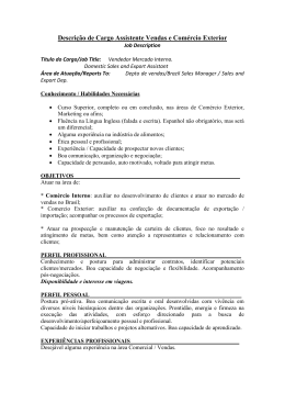
openModeller
A framework for species modeling
Fapesp process: 04/11012-0
Partial Report #1 (April 2005 – March 2006)
Introduction
The openModeller project goal is to develop a framework to facilitate the work of
scientists in predictive modeling of species distribution. The four year project
funded by Fapesp involves three institutions: CRIA (Centro de Referência em
Informação Ambiental), Poli (Escola Politécnica da USP), and INPE (Instituto
Nacional de Pesquisas Espaciais). This report summarizes the activities carried
out during the first year of the project.
Objectives and results
Most activities during the first year were related to studies and planning and,
when appropriate, included prototyping and preliminary integration. It is important
to note that an iterative and incremental development process will be used
throughout the project. This means that no attempt has been made to produce
complete or final specifications. Any specification (and also implementation) will
be revised and changed, whenever necessary, during the project lifetime. This
approach is especially convenient for complex projects when requirements,
architectural constraints, and sometimes the problem understanding may change
over time.
Below is the list of objectives proposed for the first year, followed by a summary
of activities and the main achievements during the same period.
General framework activities/studies
Evaluation of parallelization techniques and analysis of parallel algorithms for
biodiversity data analysis
A study and analysis of the current openModeller library and its performance was
conducted to assess the potential for parallelizing part of the processing. This
involved studying specific algorithms (such as GARP) and modules, such as the
Projection Module, which is processed after any modeling algorithm and is a
good candidate for being parallelized.
Considering the requirements (high job throughput and parallel processing), a
cluster of multiprocessor nodes is an appropriate computational system that will
add processing power to openModeller. Meetings were held with some
companies (Sun, Silicon, HP, IBM, Itautec, AMD and Intel) to get information
about technical and commercial features of their products. Solutions of clusters
with 2 dual-core nodes or multiprocessor nodes and Infiniband network are being
analyzed to define the best equipment for the project.
A scheduler is necessary to improve the efficiency in executing tasks in a cluster.
Some tools are available for that, such as PBS (Portable Batch System), LSF
(Load Sharing Facility), Condor and others. A study was carried out with Condor,
a tool developed at University of Wisconsin, Madison, as this tool is mature and
there are a lot of study-cases around the world. The tools and its concepts were
studied; it was installed in four machines at Poli-USP to establish a Condor Pool
for task execution. Annex 1 (condor_config.doc) and 2 (ClassAd .doc) describe
the mechanism that enables a task to be allocated to an appropriate resource,
and annex 3 (sh_loop.test .txt) has examples of tests.
Identification of general services requirements to access data and services
A series of interviews, hands-on modeling sessions and formal presentations
were made with the objective of understanding the process of species modeling.
This was very important to identify the present use-cases of the software, some
of its bottlenecks, opportunities for improvements, not only from a user-interface
point of view (software usability issues) but also from an architectural point of
view (data and processing distribution, for instance). Those activities were
beneficial for the project researchers, as they helped increase their
understanding of the users’ point of view, and were also important for the species
modelers since they had to reflect about their modeling process which
sometimes tends to be very heuristic. A document discussing the modeling
process, its activities and many issues related to them, such as data and
algorithm selection and quality can be found in annex 4 (ModelingProcess.doc).
Definition of Services Architecture
When the openModeller project was proposed, a running version of the main
library was already being developed as open-source software with its code
available at SourceForge. The development was being conducted by specialists
from CRIA, University of Kansas, and University of Reading.
As both partners INPE and Poli-USP joined the project with the support from
FAPESP, they had to study and understand the existing system, upon which the
project proposal was made, in order to know its functionalities and structure. This
was mandatory in order to propose necessary modifications on its architecture,
features, and techniques.
As in many open source initiatives, which are largely based on voluntary work
sometimes without a clear development process, there was little formal
documentation of the project, since the developers usually prefer to work only on
the code. One important activity consisted on an in-depth study of the system
and on creating some basic documents for the existing code. Reverse
engineering techniques were used which resulted in some documents that help
understand the software, the overall architecture, and its main methods and
classes. Unified Modeling Language (UML) was used and documents that were
created include use-case diagrams and class diagram (only the main diagram).
They can be seen in annex 5 (openModeller_UML.doc, partially in Portuguese).
The process of installing and configuring the development environment also
included documentation. A CD with installation instructions was created,
including source-code, libraries and a tutorial of the installation on MS Windows
environment (annex 6 - tutorial-windows.doc - in Portuguese). A tutorial on the
use of WinCVS to get the source code in a MS Windows development
environment was also prepared (annex 7 - openModeller com WinCVS.doc - in
Portuguese).
Locality data component
Defining a standard protocol between this component and a client interface,
including data formats and commands
The first step to define a locality data component was to standardize the basic
input of locality data. A new interface has been created for that purpose
(OccurrencesReader) allowing locality data to be read from simple text files or
from TerraLib tables. More documentation can be found in annex 8
(OccurrencesReader_refman.rtf). A prototype to retrieve data from GBIF1 has
also been implemented as part of the new desktop interface, and should soon be
included as a new input alternative within the component.
Next steps will include the definition of methods to expose available localities
(either stored in a TerraLib database or in specific text files) and the broadening
of input data fields that will allow usage of data-cleaning techniques.
Study of data-cleaning techniques
Several data-cleaning techniques have been implemented and studied initially as
part of the speciesLink project2 which is one of the main sources of species
occurrences data. This work continued with the openModeller project which also
benefits from high quality data. Data tests directly related to locality attributes
include:
•
•
•
1
2
Geographic error detection:
o Check that coordinates are consistent with the administrative regions
provided by the original records
o Check that coordinates are consistent with the species habitat
(marine/terrestrial)
Elevation error detection:
o Check that coordinates correspond to an elevation consistent with data
provided by the original records
Itinerary error detection:
http://www.gbif.org/
http://splink.cria.org.br/dc
•
o When records are associated to an individual (such as a collector) check
that all points from the same individual are geographically consistent with
the original collecting dates
Geographic outlier detection:
o Detect outliers on latitude and longitude using a statistical method based
on reverse-jackknifing procedure.
A data-cleaning framework called Data Tester3 was developed by CRIA and is a
strong candidate to be used by the locality component. Since the framework was
written in a different language (Java), we are currently considering the possibility
of creating a protocol to make remote invocations to a data-cleaning service.
Data Tester is a recent initiative, but there are good chances for other projects to
adopt it, which would certainly increase the number of available tests that could
be used by the locality component. It also makes more sense for some tests (like
the geographic error detection) to be run on servers that could use a library of
layers. Remote interaction between the locality component and a data-cleaning
service will be considered during the next steps.
Environmental data component
Defining a standard protocol between this component and a client interface,
including data formats and commands
The first step towards an environmental data component was to standardize
input and output of environmental data regarding the interaction with the
modeling component. This was achieved by creating a new “Raster” interface
with two initial implementations: a GDAL adapter and a TerraLib adapter. GDAL4
is a translator library for raster geospatial formats5 and TerraLib6 is a library of
GIS classes and functions that can also store rasters on relational databases.
The new Raster interface makes it possible for openModeller to read and write
raster objects using both adapters. More documentation can be found in annex 9
(Raster_refman.rtf).
Next steps will include the definition and adoption of metadata for environmental
layers and the corresponding methods to advertise which layers are available.
New ways to search and retrieve remote layers should also be investigated.
Access to local data using TerraLib
The original objective for the first year was to propose a way of integrating
openModeller with TerraLib, so that the two environments complement each
other. OpenModeller doesn’t have access to technologies that are usually found
3
http://gbif.sourceforge.net/datatester/javadoc/
http://www.remotesensing.org/gdal/
5
http://www.remotesensing.org/gdal/formats_list.html
6
http://www.terralib.org/
4
in GIS, for instance interaction with complex geographical databases and geoprocessing algorithms. On the other hand TerraLib has the tools to manage data
in geographical databases using a set of spatial and spatio-temporal data
structures; it also provides a set of spatial statistics algorithms, image processing
algorithms and functions to execute map algebra. Integration is a technique that
combines software components in order to generate more complex systems.
This technique is an efficient form of software project, saving time and resources,
and enabling the use of specialized tools in each area of the wider project.
The openModeller source code was studied and an architecture specification to
integrate the two environments was proposed considering the following aspects:
a) to impose minimum impact on both libraries; b) to allow the addition of new
functionalities as the project develops (scalability).
The proposed architecture uses a TerraLib database for information exchange
between both environments. This feature also enables close coupling with other
TerraLib based programs such as TerraView GIS or TerraWeb web application.
An initial version of the OM+TerraLib environment was built. This version allows
processing of request files using environmental maps and occurrence data
stored in a TerraLib database. Resulting maps can also be stored in a TerraLib
database. A technical report about this integration task can be found in annex 10
(TerraLib-openModeller_r1.doc, in Portuguese).
Pre-analysis component
Study of and testing pre-analysis tools
In order to increase model accuracy and improve performance during model
creation, a series of pre-processing tools have been identified as potential
candidates for being implemented. Data-cleaning techniques can also be seen
as a pre-processing step, but were omitted here (see previous section “Study of
data-cleaning techniques”).
Recent studies being carried out by CRIA (Koch, I., unpublished) show that
different sets of input layers may give completely different results. This clearly
suggests the implementation of pre-processing techniques to cross reference
occurrence points with environmental values and determine which layers can
better explain the distribution of a particular species. Such techniques include
PCA (Principal Components Analysis) and correlation tests.
Other pre-processing techniques like sub-sampling locality data into test and
training datasets are widely used by data modelers and should definitely be
implemented as part of the project to facilitate testing models that are generated.
This scenario anticipates a clear relationship between pre and post processing
components. Bootstrapping analysis requiring re-sampling of locality data was
also suggested.
Providing ways to visualize occurrence points from both the geographical and
environmental viewpoints can also be important to check if the current samples
are widely or poorly distributed in the region of interest. The initial proposal for
doing this considering the environmental dimensions is to develop a means of
estimating the basic niche conditions, therefore providing a reference to measure
how spread or concentrated are the occurrence points.
Next steps include the identification of common aspects between all these
techniques to specify a standard way of interacting with this component and then
implement the first prototypes.
Modeling component
Defining a standard protocol between this component and a client interface,
including data formats and commands
In the first year of the project, six openModeller releases were made (a change
log can be found in annex 11 - ChangeLog.txt). Since its initial version, many
changes were made to the main controller class (OpenModeller) to enable model
projection in different scenarios and also model serialization. The original design
has been gradually changed by exposing other internal classes related to
sampling, environment layers, and locality points. The C++ API to interact with
clients is now considered stable, including methods to retrieve algorithms
metadata, to set parameters (input and output layers, input and output masks,
localities data, output format, algorithm, and algorithm parameters), to create
models, to project models generating distribution maps, and to serialize and
deserialize models. The complete client API, including methods and data
formats, can be found in annex 12 (OpenModeller_refman.rtf). Additional
documentation for the whole component is available online7. This API is currently
used by a console interface, a graphical user interface (see section “Desktop
Interface”), a Python wrapper, and a SOAP interface for remote jobs.
The current algorithm API (classes AlgorithmImpl, AlgMetadata and
AlgParameter) tries to abstract the canonical modeling approach and includes
methods for initialization, model computation based on environmental values at
all occurrence points, iteration, probability calculation at specific environmental
conditions, serialization, deserialization, and metadata retrieval. Integration with
GSL (GNU Scientific Library) also enables algorithm writers to make use of a
broad range of mathematical functions8.
Adaptive Technology applied in modeling
As to the use of adaptive techniques for creating new algorithms, subsystems
have been identified and changed so that the resulting algorithm can become
7
8
http://openmodeller.cria.org.br/doxygen/0.3.4/
http://www.gnu.org/software/gsl/
adaptive, and the needed modifications can be performed. Specifically in the
“Garp” class, “mutate” and “mutatecrossover” methods were studied in order to
insert an adaptive mechanism into their basic logic. After that, adaptive
equivalent versions were designed. The implementation is expected for the
second year of the project.
As another result of our study, the exact point in which calls to any new
algorithms are to be inserted has been identified in the original source-code,
namely the “AlgoAdapterModelImpl” constructor of the “AlgoAdapterModelImpl”
class. This kind of change in the source-code will take place as soon as
operational versions of the new algorithms are available. Changes in genetic
operators were designed to include Adaptive Decision Tables, as a mechanism
of control of genetic information to be manipulated. As a partial result of this
work, adaptive versions of the genetic operators of Crossover and Mutation are
being designed. A paper is also being prepared (annex 13 - GECC02007.pdf).
Post-analysis component
Studying and testing post-analysis tools
A wide range of post-processing techniques have been identified as potential
candidates to be implemented. These include:
•
•
•
•
•
•
Validation of model results (used with the pre-processing component).
Algorithm comparison (part of a post-doctoral scholarship work plan under
analysis).
Hotspot analysis (a distribution map aggregator).
Extinction risk analysis (considering distribution maps for different time
scenarios).
Methods for describing and exploring reasons for distribution.
Methods for tuning parameters settings (comparing the effects of different
parameter values in model results as a way to discover general criteria for
choosing optimal parameter values).
Next steps include the identification of common aspects between all these
techniques to specify a standard way of interacting with this component and then
implement the first prototypes.
Desktop Interface
During the last year, releases 0.3.1 and 0.3.2 of the existing openModeller
graphical user interface were made, including improvements and bug fixes.
Although the existing interface has been a successful step toward making the
library widely accessible to the general public, it became clear that it only
covered the basic needs of researchers through a wizard-like interface - a stepby-step process for running simple modeling experiments9.
Within the scope of the project, a new strategy was conceived in order to create
a more advanced and comprehensive graphical user interface that will enable
researchers to carry out complex experiments involving multiple species, multiple
algorithms, different environment scenarios, pre and post processing tools, and
other features. An initial list of requirements has been prepared in collaboration
with the BiodiversityWorld project researchers, as well as the first mock-ups10.
The current strategy is to make a last release during the next weeks using the
existing code base, where multi-species modeling is already implemented. At the
same time, a next GUI generation of openModeller is under work using Qt4
instead of Qt3 (Qt11 is the graphical library being used by the interface). This new
major version will be an intermediary step to reach the final and advanced
version, and it will serve as a test bed for the new openModeller components.
This intermediary version includes a locality data component capable of getting
local data from text files and retrieving remote data from GBIF servers. An initial
version for a simple environmental data component will also be able to show both
local and remote map directories. A modeling adapter will enable usage of either
a local openModeller instance or a remote openModeller server (potentially
making use of a cluster). Initial implementations of additional tools for postprocessing analysis like producing hotspots maps are also being developed. This
new interface is under active work and its first release is planned for July 2006.
By that time, when most changes in Qt4 will be assimilated and a greater
understanding of the new openModeller framework components will be achieved,
a third and final generation of graphical user interface will follow. This should be
the advanced interface addressing all necessary requirements and making the
final integration between all framework components. Interaction with different GIS
should also be possible through a common plug-in adapter. It is important to
mention that a considerable part from both previous code bases will be reused
(the wizard interface will remain an option for new users, and the initial versions
of framework components that were developed in the intermediary generation will
be improved to gain full functionality).
Web Interface
9
http://sourceforge.net/project/showfiles.php?group_id=101808&package_id=142057&release_id=348560
10
http://openmodeller.cria.org.br/wikis/omgui/ScreenShots?action=AttachFile&do=view&target=omGui2Scr
eenShotA.png
11
http:///www.trolltech.com/
A first prototype for an openModeller web interface has been developed12. This
interface has access control (also depends on prior user registration on the
server side) and it currently enables users to:
•
•
•
•
•
•
Create and run new modeling jobs
Display job status
List all jobs created by the user
Delete jobs
Visualize distribution maps through the web
Save distribution maps as local files
This interface was developed using Perl scripts and is initially making use of the
openModeller command line tool (om_console). To run a new job, users follow a
step by step process specifying each parameter. The list of algorithms and their
respective parameters are still hard coded. Users can upload text files with
locality data and can choose environmental layers located on the server.
Additional parameters like masks and projection are selected from pre-defined
options. After specifying all parameters, the script builds a request file suitable for
"om_console" ingestion and then monitors the process status.
A generic mapping application has been developed to visualize maps on the
web. This application includes a set of scripts that communicate with a web
service. More documentation can be found in annex 14 (mapCRIA.doc).
When the new framework components are fully implemented, the idea is to wrap
them using SWIG13 to make their functionality directly available from scripting
languages like Python, Perl and PHP. Although it is also possible to build C++
CGI programs, those scripting languages are more widely used in the Internet
environment. The next versions of this interface will therefore import specific
modules generated by SWIG and then interact directly with each framework
component.
Study Cases
According to the project timeline proposed, study cases were planned to initiate
in the second year to test and improve the framework and also to prove the
concept. They included testing different environmental data to achieve better
results and optimize modeling procedures; testing different algorithms to analyze
which are the best for what combination of data and species; applying knowledge
from modeling in techniques that help conservation of species and in the
recuperation of degraded areas; and developing modeling techniques for species
with very few occurrence data. CRIA and INPE have interest in case studies in
the Cerrado, Amazon, São Paulo State and in the Iriri area of Xingu.
12
13
http://openmodeller.cria.org.br/criamodeller/
http://www.swig.org/
(login: guest password: guest)
A research schedule is under preparation to enable the development of Study
Cases. The main activities developed during the first year were:
•
A research proposal to assess sensitivity of species distribution models
(SDM) to different precisions in the geographic position of occurrence
data: Modeling algorithms implemented in openModeller, such as GARP
and BIOCLIM, and other algorithms, like ENFA, GLM and Maxent, will be
evaluated. Fábio Iwashita’s thesis proposition (annex 15 Iwashita_Proposal.pdf – in Portuguese) describes the details.
•
A research project to be submitted as a Pos-Doctoral activity at INPE to
study and discuss the relationship between phylogenetic diversity and
spatial distribution in the Amazon region: Collaboration with Dra. Lucia
Lohmann (USP) will provide access to a Bignoniaceae database
containing georeferenced occurrence data for the species (to generate the
distribution models) and the cladograms with taxonomic hierarchies (to
obtain the phylogenetic diversity indexes). Spatial analysis of the species
distribution and the phylogenetic diversity patterns will contribute to the
discussion about the biogeographical theories and will provide a new
approach to conservation strategies. Cristina B. Costa’s thesis proposition
(annex 16 - Costa_PosDoc.pdf – in Portuguese) describes more details.
•
Development of a geographical database using the TerraLib storage
mechanisms to explore the influence of environmental data on the
modeling process: Besides the environmental data usually considered for
species distribution modeling (and available in the internet) we are
including climatic data from CPTEC-INPE, remote sensing imagery, and
other maps describing the biophysical environment. Species of
Rubiaceae, from the genus Coccocypselum, will be used to test the
effects of environmental data on distribution models. We intend to discuss
the conservation aspect, considering the genus distribution and diversity,
and also regarding the conservation units already established in the
Brazilian territory. This activity is already providing data to test the
openModeller-TerraLib integration.
Other relevant activities and results
Development of the aRT package
Statistical spatial data analysis and Geographical Information Systems
(GIS) can act together in order to understand and model spatially distributed
data. Geoprocessing operations can equip statistical models with relevant
information which can be used to better understand the main features of usually
noisy and multidimensional data. Therefore integration between GIS and
statistical software can be highly beneficial for both sides. The package aRT14
enables the access to TerraLib from the statistical software called R15. aRT
encapsulates C++ classes into S4, therefore the user can manipulate TerraLib
objects directly in memory using the implemented wrappers. aRT can manipulate
spatial data using the data structures of the sp package, reading and writing
Spatial data in the database. Some spatial operations already implemented in the
package as part of this project are:
•
•
•
Manipulation of points, lines, polygons and raster data;
Spatial predicates, such as “touches”, “within”, “contains”, “crosses” and
“overlaps”;
Polygons operations, as “union”, “intersection”, “difference” and
“simplification”.
aRT is available as source code and also as a cross-compiled Windows binary.
Along with the package, there are files documenting the implemented functions
and also examples of scripts showing how to use aRT.
Setting up a project portal
Although openModeller's source code is available at SourceForge, there was a
need to have an environment for all the project participants to share information,
such as presentations, papers, data, project management documents (meetings
memos, etc.). The FAPESP’s Incubadora Virtual de Projetos (Projects Virtual
Incubator) provides an environment for the creation of project portals that can
host both public and private content, besides providing many services such as
news, calendar, mailing lists, etc. A portal for the openModeller project was
created, after being approved by Incubadora’s managers and can be used by all
the project community16.
Changes in the original aims
For the first year, the project originally proposed to define standard protocols
between all components and a generic client interface, including data formats
and commands. Unfortunately it was not possible to achieve this for some of the
components (especially the pre and post processing components). This was
mainly caused by the usual difficulties that happen during the first year of a
complex project when setting up a working team and finding efficient ways to
collaborate across different institutions. The intention is to achieve these goals
during the second year of the project.
The study cases originally prioritized the following areas: Cerrado, Amazon
region, São Paulo State, and Xingu-Iriri. We are sustaining the same targets
14
http://www.est.ufpr.br/aRT
http://www.r-project.org/
16
http://openmodeller.incubadora.fapesp.br/
15
except for Xingu-Iriri due to significant difficulties in obtaining reliable species
occurrence data for that area. The region of Marajó-Tocantins was chosen as an
alternative study site.
Workshops
On February 2006 all developers were invited to participate in a “code fest”17 at
CRIA to explore the existing common interests between openModeller and the
BiodiversityWorld project18. Two representatives from BDWorld attended: Tim
Sutton and Peter Brewer. The main goals were to:
•
•
•
•
•
Review requirements and desirable features for an advanced openModeller
graphical user interface.
Produce an API specification for remote invocation of openModeller jobs.
Start implementing the next generation of a graphical user interface for
openModeller.
Document the release process for both openModeller and its GUI, in
particular under the Windows platform, and release omgui 0.3.4.
Familiarize new developers with the openModeller development environment.
The BDWorld project has a Condor cluster already prepared to run openModeller
jobs and is therefore interested in providing interfaces to it. The next generation
of an openModeller graphical user interface will be able to seamlessly run either
local or remote openModeller jobs, opening new perspectives for the scientific
community. The same interface should be able to use a new openModeller
cluster to be installed at Escola Politécnica da USP as part of this project.
Significant advances were achieved during the meeting, when it was decided to
use the SOAP protocol with “Document” mode and “Literal” encoding combined
with openModeller serialization/deserialization capabilities. The first prototypes
for remote invocation methods were implemented (method
GetAvailableAlgorithms) and a full featured version should be released during
2006.
Publications and Presentations
Andrade Neto, P. R., Justiniano Jr., P. R. and Fook, K. D., Integration of
Statistics and Geographic Information Systems: the R/TerraLib Case. VII
Brazilian Symposium on GeoInformatics, GeoInfo2005. Campos do Jordão, SP,
Brazil, 2005.
Andrade Neto, P. R. and Justiniano Jr., P. R., A Process and Environment for
Embedding the R Software into TerraLib. VII Brazilian Symposium on
GeoInformatics, GeoInfo2005. Campos do
17
18
http://openmodeller.cria.org.br/wikis/om/February2006CodeFest
http://www.bdworld.org/
Jordão, SP, Brazil, 2005.
Bonaccorso, E.; Koch, I. & Peterson, A.T. (in press). Pleistocene fragmentation
of Amazon species' ranges. Diversity and Distributions.
Chapman, A.D.; Muñoz, M.E.S. & Koch, I. 2005. Environmental Information:
Placing Biodiversity Phenomena in an Ecological and Environmental Context.
Biodiversity Informatics, 2, 2005, pp. 24-41. Available at:
http://jbi.nhm.ku.edu/viewarticle.php?, August, 2005.
Canhos, V. P., at al., 2005. The speciesLink Network: practical solutions for
integrating, analyzing, sinthesizing and visualizing Biodiversity Information. First
Diversitas Open Science Conference, Oaxaca, Mexico, November 2005.
Giovanni, R., 2005. openModeller: A new tool for fundamental niche modelling.
BDWorld Workshop, National e-Science Centre, Edinburgh, UK, June 2005.
Koch, I.; Peterson, A.T. & Shepherd, G. (in preparation). Distribuição geográfica
potencial de espécies de Rauvolfia (apocynaceae) e projeções para cenários
climáticos do passado.
Koch, I.; Peterson, A.T. & Shepherd, G. 2005. Distribuição geográfica potencial
de espécies de Rauvolfia (apocynaceae) e projeções para cenários climáticos do
passado. 56º. Congresso Nacional de Botânica, Curitiba, PR, Outubro 2005.
Koch, I.; Shepherd, G.J. & Siqueira, M.F. (in preparation). Modelagem de
Distribuição Geográfica Potencial de Espécies de Apocynaceae no Estado de
São Paulo.
Meireles, L.D.; Shepherd, G.J.; Koch, I. & Siqueira, M.F. 2005. Modelagem da
distribuição geográfica de Araucaria angustifolia com projeções para cenários
climáticos do passado. 56º. Congresso Nacional de Botânica, Curitiba, PR,
Outubro 2005.
Neto, J. J., Bravo, C., Adaptive Version of Crossover and Mutation Genetic
Operators for the GARP Algorithm (annex 13 - GECC02007.pdf). Summary and
status: discusses a method for obtaining adaptive versions for Crossover and
Mutation genetic operators in the GARP algorithm. Paper in preparation to be
submitted to GECCO-2007 - Genetic and Evolutionary Computation Conference.
Santana, F. S., Fonseca, R. R., Saraiva, A. M., Corrêa, P. L. P., Bravo, C.,
Giovanni, R., openModeller - an open framework for ecological niche modeling:
analysis and future improvements (annex 17 - 2006 WCCA Presentation
Proposal.doc). Summary and status: describes current openModeller
implementation and discusses further improvements. 50% completed. Submitted
to and accepted by the 2006 WCCA - World Conference on Computers in
Agriculture and Natural Resources.
Santana, F. S., Siqueira, M.F. & Saraiva, A. M. (in preparation). Modeling of
species distribution based on fundamental niche concepts: the generation of
geographic distribution models using openModeller. (annex 4 –
ModelingProcess.doc). Summary and status: describes the process of model
generation using Open Modeller. 80% completed. Yet to be submitted to a
scientific journal.
Siqueira, M.F. & Durigan, G. (submitted). Modelagem de Espécies Lenhosas
para a Região de Cerrado no Estado de São Paulo. Revista Brasileira de
Botânica.
Siqueira, M.F., Durigan, G., de Marco Jr, P. & Peterson, A. T. (in preparation).
Something from Nothing: Using Landscape Similarity and Ecological Niche
Modeling to Find Rare Plant Species.
Siqueira, M.F., Durigan, G. & Marco Jr, P. (in preparation) Aplicações de
modelagem para auxiliar trabalhos de recuperação ambiental.
Annex 01
##################################################################
####
##
## condor_config
##
## This is the global configuration file for condor.
##
## The file is divided into four main parts:
## Part 1: Settings you MUST customize
## Part 2: Settings you may want to customize
## Part 3: Settings that control the policy of when condor will
##
start and stop jobs on your machines
## Part 4: Settings you should probably leave alone (unless you
## know what you're doing)
##
## Please read the INSTALL file (or the Install chapter in the
## Condor Administrator's Manual) for detailed explanations of the
## various settings in here and possible ways to configure your
## pool.
##
## If you are installing Condor as root and then handing over the
## administration of this file to a person you do not trust with
## root access, please read the Installation chapter paying careful
## note to the condor_config.root entries.
##
## Unless otherwise specified, settings that are commented out show
## the defaults that are used if you don't define a value. Settings
## that are defined here MUST BE DEFINED since they have no default
## value.
##
## Unless otherwise indicated, all settings which specify a time are
## defined in seconds.
##
##################################################################
####
##################################################################
####
##################################################################
####
## Part 1: Settings you must customize:
##################################################################
####
##################################################################
####
## What machine is your central manager?
CONDOR_HOST
= g1.mygrid
##-------------------------------------------------------------------## Pathnames:
##-------------------------------------------------------------------## Where have you installed the bin, sbin and lib condor directories?
RELEASE_DIR
= /usr/local/condor
## Where is the local condor directory for each host?
LOCAL_DIR
= $(TILDE)
#LOCAL_DIR
=
$(RELEASE_DIR)/hosts/$(HOSTNAME)
## Where is the machine-specific local config file for each host?
LOCAL_CONFIG_FILE
= $(LOCAL_DIR)/condor_config.local
#LOCAL_CONFIG_FILE = $(RELEASE_DIR)/etc/$(HOSTNAME).local
## If the local config file is not present, is it an error?
## WARNING: This is a potential security issue.
## If not specificed, te default is True
#REQUIRE_LOCAL_CONFIG_FILE = TRUE
##-------------------------------------------------------------------## Mail parameters:
##-------------------------------------------------------------------## When something goes wrong with condor at your site, who should get
## the email?
CONDOR_ADMIN
= [email protected]
## Full path to a mail delivery program that understands that "-s"
## means you want to specify a subject:
MAIL
= /bin/mail
##-------------------------------------------------------------------## Network domain parameters:
##-------------------------------------------------------------------## Internet domain of machines sharing a common UID space. If your
## machines don't share a common UID space, use the second entry
## which specifies that each machine has its own UID space.
UID_DOMAIN
= $(FULL_HOSTNAME)
#UID_DOMAIN
= $(FULL_HOSTNAME)
## Internet domain of machines sharing a common file system.
## If your machines don't use a network file system, use the second
## entry which specifies that each machine has its own file system.
FILESYSTEM_DOMAIN = $(FULL_HOSTNAME)
#FILESYSTEM_DOMAIN = $(FULL_HOSTNAME)
##################################################################
####
##################################################################
####
## Part 2: Settings you may want to customize:
## (it is generally safe to leave these untouched)
##################################################################
####
##################################################################
####
##-------------------------------------------------------------------## Flocking: Submitting jobs to more than one pool
##-------------------------------------------------------------------## Flocking allows you to run your jobs in other pools, or lets
## others run jobs in your pool.
##
## To let others flock to you, define FLOCK_FROM.
##
## To flock to others, define FLOCK_TO.
## FLOCK_FROM defines the machines where you would like to grant
## people access to your pool via flocking. (i.e. you are granting
## access to these machines to join your pool).
FLOCK_FROM =
## An example of this is:
#FLOCK_FROM = somehost.friendly.domain, anotherhost.friendly.domain
## FLOCK_TO defines the central managers of the pools that you want
## to flock to. (i.e. you are specifying the machines that you
## want your jobs to be negotiated at -- thereby specifying the
## pools they will run in.)
FLOCK_TO =
## An example of this is:
#FLOCK_TO = central_manager.friendly.domain, condor.cs.wisc.edu
## FLOCK_COLLECTOR_HOSTS should almost always be the same as
## FLOCK_NEGOTIATOR_HOSTS (as shown below). The only reason it
would be
## different is if the collector and negotiator in the pool that you are
## flocking too are running on different machines (not recommended).
## The collectors must be specified in the same corresponding order as
## the FLOCK_NEGOTIATOR_HOSTS list.
FLOCK_NEGOTIATOR_HOSTS = $(FLOCK_TO)
FLOCK_COLLECTOR_HOSTS = $(FLOCK_TO)
## An example of having the negotiator and the collector on different
## machines is:
#FLOCK_NEGOTIATOR_HOSTS = condor.cs.wisc.edu, condornegotiator.friendly.domain
#FLOCK_COLLECTOR_HOSTS = condor.cs.wisc.edu, condorcollector.friendly.domain
##-------------------------------------------------------------------## Host/IP access levels
##-------------------------------------------------------------------## Please see the administrator's manual for details on these
## settings, what they're for, and how to use them.
## What machines have administrative rights for your pool? This
## defaults to your central manager. You should set it to the
## machine(s) where whoever is the condor administrator(s) works
## (assuming you trust all the users who log into that/those
## machine(s), since this is machine-wide access you're granting).
HOSTALLOW_ADMINISTRATOR = $(CONDOR_HOST)
## If there are no machines that should have administrative access
## to your pool (for example, there's no machine where only trusted
## users have accounts), you can uncomment this setting.
## Unfortunately, this will mean that administering your pool will
## be more difficult.
#HOSTDENY_ADMINISTRATOR = *
## What machines should have "owner" access to your machines, meaning
## they can issue commands that a machine owner should be able to
## issue to their own machine (like condor_vacate). This defaults to
## machines with administrator access, and the local machine. This
## is probably what you want.
HOSTALLOW_OWNER = $(FULL_HOSTNAME),
$(HOSTALLOW_ADMINISTRATOR)
## Read access. Machines listed as allow (and/or not listed as deny)
## can view the status of your pool, but cannot join your pool
## or run jobs.
## NOTE: By default, without these entries customized, you
## are granting read access to the whole world. You may want to
## restrict that to hosts in your domain. If possible, please also
## grant read access to "*.cs.wisc.edu", so the Condor developers
## will be able to view the status of your pool and more easily help
## you install, configure or debug your Condor installation.
## It is important to have this defined.
HOSTALLOW_READ = *
#HOSTALLOW_READ = *.your.domain, *.cs.wisc.edu
#HOSTDENY_READ = *.bad.subnet, bad-machine.your.domain, 144.77.88.*
## Write access. Machines listed here can join your pool, submit
## jobs, etc. Note: Any machine which has WRITE access must
## also be granted READ access. Granting WRITE access below does
## not also automatically grant READ access; you must change
## HOSTALLOW_READ above as well.
## If you leave it as it is, it will be unspecified, and effectively
## it will be allowing anyone to write to your pool.
HOSTALLOW_WRITE = *
#HOSTALLOW_WRITE = *.your.domain, your-friend's-machine.other.domain
#HOSTDENY_WRITE = bad-machine.your.domain
## Negotiator access. Machines listed here are trusted central
## managers. You should normally not have to change this.
HOSTALLOW_NEGOTIATOR = $(NEGOTIATOR_HOST)
## Now, with flocking we need to let the SCHEDD trust the other
## negotiators we are flocking with as well. You should normally
## not have to change this either.
HOSTALLOW_NEGOTIATOR_SCHEDD = $(NEGOTIATOR_HOST),
$(FLOCK_NEGOTIATOR_HOSTS)
## Config access. Machines listed here can use the condor_config_val
## tool to modify all daemon configurations except those specified in
## the condor_config.root file. This level of host-wide access
## should only be granted with extreme caution. By default, config
## access is denied from all hosts.
#HOSTALLOW_CONFIG = trusted-host.your.domain
## Flocking Configs. These are the real things that Condor looks at,
## but we set them from the FLOCK_FROM/TO macros above. It is safe
## to leave these unchanged.
HOSTALLOW_WRITE_COLLECTOR = $(HOSTALLOW_WRITE),
$(FLOCK_FROM)
HOSTALLOW_WRITE_STARTD = $(HOSTALLOW_WRITE),
$(FLOCK_FROM)
HOSTALLOW_READ_COLLECTOR = $(HOSTALLOW_READ),
$(FLOCK_FROM)
HOSTALLOW_READ_STARTD = $(HOSTALLOW_READ),
$(FLOCK_FROM)
##-------------------------------------------------------------------## Security parameters for setting configuration values remotely:
##-------------------------------------------------------------------## These parameters define the list of attributes that can be set
## remotely with condor_config_val for the security access levels
## defined above (for example, WRITE, ADMINISTRATOR, CONFIG, etc).
## Please see the administrator's manual for futher details on these
## settings, what they're for, and how to use them. There are no
## default values for any of these settings. If they are not
## defined, no attributes can be set with condor_config_val.
## Attributes that can be set by hosts with "CONFIG" permission (as
## defined with HOSTALLOW_CONFIG and HOSTDENY_CONFIG above).
## The commented-out value here was the default behavior of Condor
## prior to version 6.3.3. If you don't need this behavior, you
## should leave this commented out.
#SETTABLE_ATTRS_CONFIG = *
## Attributes that can be set by hosts with "ADMINISTRATOR"
## permission (as defined above)
#SETTABLE_ATTRS_ADMINISTRATOR = *_DEBUG, MAX_*_LOG
## Attributes that can be set by hosts with "OWNER" permission (as
## defined above) NOTE: any Condor job running on a given host will
## have OWNER permission on that host by default. If you grant this
## kind of access, Condor jobs will be able to modify any attributes
## you list below on the machine where they are running. This has
## obvious security implications, so only grant this kind of
## permission for custom attributes that you define for your own use
## at your pool (custom attributes about your machines that are
## published with the STARTD_EXPRS setting, for example).
#SETTABLE_ATTRS_OWNER = your_custom_attribute, another_custom_attr
## You can also define daemon-specific versions of each of these
## settings. For example, to define settings that can only be
## changed in the condor_startd's configuration by hosts with OWNER
## permission, you would use:
#STARTD_SETTABLE_ATTRS_OWNER = your_custom_attribute_name
##-------------------------------------------------------------------## Network filesystem parameters:
##-------------------------------------------------------------------## Do you want to use NFS for file access instead of remote system
## calls?
#USE_NFS
= False
## Do you want to use AFS for file access instead of remote system
## calls?
#USE_AFS
= False
##-------------------------------------------------------------------## Checkpoint server:
##-------------------------------------------------------------------## Do you want to use a checkpoint server if one is available? If a
## checkpoint server isn't available or USE_CKPT_SERVER is set to
## False, checkpoints will be written to the local SPOOL directory on
## the submission machine.
#USE_CKPT_SERVER
= True
## What's the hostname of this machine's nearest checkpoint server?
#CKPT_SERVER_HOST
= checkpoint-server-hostname.your.domain
## Do you want the starter on the execute machine to choose the
## checkpoint server? If False, the CKPT_SERVER_HOST set on
## the submit machine is used. Otherwise, the CKPT_SERVER_HOST set
## on the execute machine is used. The default is true.
#STARTER_CHOOSES_CKPT_SERVER = True
##-------------------------------------------------------------------## Miscellaneous:
##-------------------------------------------------------------------## Try to save this much swap space by not starting new shadows.
## Specified in megabytes.
#RESERVED_SWAP
=5
## What's the maximum number of jobs you want a single submit machine
## to spawn shadows for?
#MAX_JOBS_RUNNING = 200
## Condor needs to create a few lock files to synchronize access to
## various log files. Because of problems we've had with network
## filesystems and file locking over the years, we HIGHLY recommend
## that you put these lock files on a local partition on each
## machine. If you don't have your LOCAL_DIR on a local partition,
## be sure to change this entry. Whatever user (or group) condor is
## running as needs to have write access to this directory. If
## you're not running as root, this is whatever user you started up
## the condor_master as. If you are running as root, and there's a
## condor account, it's probably condor. Otherwise, it's whatever
## you've set in the CONDOR_IDS environment variable. See the Admin
## manual for details on this.
LOCK
= $(LOG)
## If you don't use a fully qualified name in your /etc/hosts file
## (or NIS, etc.) for either your official hostname or as an alias,
## Condor wouldn't normally be able to use fully qualified names in
## places that it'd like to. You can set this parameter to the
## domain you'd like appended to your hostname, if changing your host
## information isn't a good option. This parameter must be set in
## the global config file (not the LOCAL_CONFIG_FILE from above).
#DEFAULT_DOMAIN_NAME = your.domain.name
## Condor can be told whether or not you want the Condor daemons to
## create a core file if something really bad happens. This just
## sets the resource limit for the size of a core file. By default,
## we don't do anything, and leave in place whatever limit was in
## effect when you started the Condor daemons. If this parameter is
## set and "True", we increase the limit to as large as it gets. If
## it's set to "False", we set the limit at 0 (which means that no
## core files are even created). Core files greatly help the Condor
## developers debug any problems you might be having.
#CREATE_CORE_FILES = True
## Condor Glidein downloads binaries from a remote server for the
## machines into which you're gliding. This saves you from manually
## downloading and installing binaries for every architecture you
## might want to glidein to. The default server is one maintained at
## The University of Wisconsin. If you don't want to use the UW
## server, you can set up your own (it needs to be running a gsiftp
## daemon) and change the following values to point to it, instead.
GLIDEIN_SERVER_NAME = gridftp.cs.wisc.edu
GLIDEIN_SERVER_DIR = /p/condor/public/binaries/glidein
## If your site needs to use UID_DOMAIN settings (defined above) that
## are not real Internet domains that match the hostnames, you can
## tell Condor to trust whatever UID_DOMAIN a submit machine gives to
## the execute machine and just make sure the two strings match. The
## default for this setting is False, since it is more secure this
## way.
#TRUST_UID_DOMAIN = False
##-------------------------------------------------------------------## Settings that control the daemon's debugging output:
##--------------------------------------------------------------------
##
## The flags given in ALL_DEBUG are shared between all daemons.
##
ALL_DEBUG
MASTER_DEBUG
= D_COMMAND
## When the master starts up, should it truncate it's log file?
#TRUNC_MASTER_LOG_ON_OPEN
= False
=
MAX_COLLECTOR_LOG = 1000000
COLLECTOR_DEBUG
=
MAX_KBDD_LOG
KBDD_DEBUG
= 1000000
=
MAX_NEGOTIATOR_LOG = 1000000
NEGOTIATOR_DEBUG
= D_MATCH
MAX_NEGOTIATOR_MATCH_LOG = 1000000
MAX_SCHEDD_LOG
SCHEDD_DEBUG
= 1000000
= D_COMMAND
MAX_SHADOW_LOG
SHADOW_DEBUG
= 1000000
=
MAX_STARTD_LOG
STARTD_DEBUG
= 1000000
= D_COMMAND
MAX_STARTER_LOG
STARTER_DEBUG
= 1000000
= D_NODATE
MAX_MASTER_LOG
= 1000000
##################################################################
####
##################################################################
####
## Part 3: Settings control the policy for running, stopping, and
## periodically checkpointing condor jobs:
##################################################################
####
##################################################################
####
## This section contains macros are here to help write legible
## expressions:
MINUTE
= 60
HOUR
= (60 * $(MINUTE))
StateTimer
= (CurrentTime - EnteredCurrentState)
ActivityTimer = (CurrentTime - EnteredCurrentActivity)
ActivationTimer = (CurrentTime - JobStart)
LastCkpt
= (CurrentTime - LastPeriodicCheckpoint)
## The JobUniverse attribute is just an int. These macros can be
## used to specify the universe in a human-readable way:
STANDARD = 1
PVM = 4
Annex 02
ClassAd
MyType = "Machine"
TargetType = "Job"
Name = "g1.mygrid"
Machine = "g1.mygrid"
Rank = 0.000000
CpuBusy = ((LoadAvg - CondorLoadAvg) >= 0.500000)
COLLECTOR_HOST_STRING = "g1.mygrid"
CondorVersion = "$CondorVersion: 6.6.10 Jun 13 2005 $"
CondorPlatform = "$CondorPlatform: I386-LINUX_RH80 $"
VirtualMachineID = 1
VirtualMemory = 522104
Disk = 736212
CondorLoadAvg = 0.000000
LoadAvg = 0.080000
KeyboardIdle = 0
ConsoleIdle = 0
Memory = 123
Cpus = 1
StartdIpAddr = "<192.168.100.100:1082>"
Arch = "INTEL"
OpSys = "LINUX"
UidDomain = "g1.mygrid"
FileSystemDomain = "g1.mygrid"
Subnet = "192.168.100"
HasIOProxy = TRUE
TotalVirtualMemory = 522104
TotalDisk = 736212
KFlops = 700680
Mips = 2371
LastBenchmark = 1140027198
TotalLoadAvg = 0.080000
TotalCondorLoadAvg = 0.000000
ClockMin = 988
ClockDay = 3
TotalVirtualMachines = 1
HasFileTransfer = TRUE
HasMPI = TRUE
HasJICLocalConfig = TRUE
HasJICLocalStdin = TRUE
HasPVM = TRUE
HasRemoteSyscalls = TRUE
HasCheckpointing = TRUE
StarterAbilityList =
"HasFileTransfer,HasMPI,HasJICLocalConfig,HasJICLocalStdin,HasPVM,HasRemoteSyscalls,HasCh
eckpointing"
CpuBusyTime = 0
CpuIsBusy = FALSE
State = "Owner"
EnteredCurrentState = 1140027193
Activity = "Idle"
EnteredCurrentActivity = 1140027193
Start = ((KeyboardIdle > 15 * 60) && (((LoadAvg - CondorLoadAvg) <= 0.300000) || (State
!= "Unclaimed" && State != "Owner")))
Requirements = START
CurrentRank = 0.000000
DaemonStartTime = 1140027192
UpdateSequenceNumber = 3
MyAddress = "<192.168.100.100:1082>"
LastHeardFrom = 1140028102
UpdatesTotal = 4
UpdatesSequenced = 3
UpdatesLost = 0
UpdatesHistory = "0x00000000000000000000000000000000"
Annex 03
...
000 (005.000.000) 02/16 02:35:56 Job submitted from host: <192.168.100.100:1028>
...
000 (005.001.000) 02/16 02:35:56 Job submitted from host: <192.168.100.100:1028>
...
000 (005.002.000) 02/16 02:35:56 Job submitted from host: <192.168.100.100:1028>
...
000 (005.003.000) 02/16 02:35:56 Job submitted from host: <192.168.100.100:1028>
...
000 (005.004.000) 02/16 02:35:56 Job submitted from host: <192.168.100.100:1028>
...
000 (005.005.000) 02/16 02:35:56 Job submitted from host: <192.168.100.100:1028>
...
000 (005.006.000) 02/16 02:35:56 Job submitted from host: <192.168.100.100:1028>
...
000 (005.007.000) 02/16 02:35:56 Job submitted from host: <192.168.100.100:1028>
...
000 (005.008.000) 02/16 02:35:56 Job submitted from host: <192.168.100.100:1028>
...
000 (005.009.000) 02/16 02:35:56 Job submitted from host: <192.168.100.100:1028>
...
000 (005.010.000) 02/16 02:35:56 Job submitted from host: <192.168.100.100:1028>
...
000 (005.011.000) 02/16 02:35:56 Job submitted from host: <192.168.100.100:1028>
...
000 (005.012.000) 02/16 02:35:56 Job submitted from host: <192.168.100.100:1028>
...
000 (005.013.000) 02/16 02:35:56 Job submitted from host: <192.168.100.100:1028>
...
000 (005.014.000) 02/16 02:35:56 Job submitted from host: <192.168.100.100:1028>
...
000 (005.015.000) 02/16 02:35:56 Job submitted from host: <192.168.100.100:1028>
...
000 (005.016.000) 02/16 02:35:56 Job submitted from host: <192.168.100.100:1028>
...
000 (005.017.000) 02/16 02:35:56 Job submitted from host: <192.168.100.100:1028>
...
000 (005.018.000) 02/16 02:35:56 Job submitted from host: <192.168.100.100:1028>
...
000 (005.019.000) 02/16 02:35:56 Job submitted from host: <192.168.100.100:1028>
...
000 (006.000.000) 02/16 02:35:57 Job submitted from host: <192.168.100.100:1028>
...
000 (006.001.000) 02/16 02:35:57 Job submitted from host: <192.168.100.100:1028>
...
000 (006.002.000) 02/16 02:35:57 Job submitted from host: <192.168.100.100:1028>
...
000 (006.003.000) 02/16 02:35:57 Job submitted from host: <192.168.100.100:1028>
...
000 (006.004.000) 02/16 02:35:57 Job submitted from host: <192.168.100.100:1028>
...
000 (006.005.000) 02/16 02:35:57 Job submitted from host: <192.168.100.100:1028>
...
000 (006.006.000) 02/16 02:35:57 Job submitted from host: <192.168.100.100:1028>
...
000 (006.007.000) 02/16 02:35:57 Job submitted from host: <192.168.100.100:1028>
...
000 (006.008.000) 02/16 02:35:57 Job submitted from host: <192.168.100.100:1028>
...
000 (006.009.000) 02/16 02:35:57 Job submitted from host: <192.168.100.100:1028>
...
000 (006.010.000) 02/16 02:35:57 Job submitted from host: <192.168.100.100:1028>
...
000 (006.011.000) 02/16 02:35:57 Job submitted from host: <192.168.100.100:1028>
...
000 (006.012.000) 02/16 02:35:57 Job submitted from host: <192.168.100.100:1028>
...
000 (006.013.000) 02/16 02:35:57 Job submitted from host: <192.168.100.100:1028>
...
000 (006.014.000) 02/16 02:35:57 Job submitted from host: <192.168.100.100:1028>
...
000 (006.015.000) 02/16 02:35:57 Job submitted from host: <192.168.100.100:1028>
...
000 (006.016.000) 02/16 02:35:57 Job submitted from host: <192.168.100.100:1028>
...
000 (006.017.000) 02/16 02:35:57 Job submitted from host: <192.168.100.100:1028>
...
000 (006.018.000) 02/16 02:35:57 Job submitted from host: <192.168.100.100:1028>
...
000 (006.019.000) 02/16 02:35:57 Job submitted from host: <192.168.100.100:1028>
...
000 (007.000.000) 02/16 02:35:58 Job submitted from host: <192.168.100.100:1028>
...
000 (007.001.000) 02/16 02:35:58 Job submitted from host: <192.168.100.100:1028>
...
000 (007.002.000) 02/16 02:35:58 Job submitted from host: <192.168.100.100:1028>
...
000 (007.003.000) 02/16 02:35:58 Job submitted from host: <192.168.100.100:1028>
...
000 (007.004.000) 02/16 02:35:58 Job submitted from host: <192.168.100.100:1028>
...
000 (007.005.000) 02/16 02:35:58 Job submitted from host: <192.168.100.100:1028>
...
000 (007.006.000) 02/16 02:35:58 Job submitted from host: <192.168.100.100:1028>
...
000 (007.007.000) 02/16 02:35:58 Job submitted from host: <192.168.100.100:1028>
...
000 (007.008.000) 02/16 02:35:58 Job submitted from host: <192.168.100.100:1028>
...
000 (007.009.000) 02/16 02:35:58 Job submitted from host: <192.168.100.100:1028>
...
000 (007.010.000) 02/16 02:35:58 Job submitted from host: <192.168.100.100:1028>
...
000 (007.011.000) 02/16 02:35:58 Job submitted from host: <192.168.100.100:1028>
...
000 (007.012.000) 02/16 02:35:58 Job submitted from host: <192.168.100.100:1028>
...
000 (007.013.000) 02/16 02:35:58 Job submitted from host: <192.168.100.100:1028>
...
000 (007.014.000) 02/16 02:35:58 Job submitted from host: <192.168.100.100:1028>
...
000 (007.015.000) 02/16 02:35:58 Job submitted from host: <192.168.100.100:1028>
...
000 (007.016.000) 02/16 02:35:58 Job submitted from host: <192.168.100.100:1028>
...
000 (007.017.000) 02/16 02:35:58 Job submitted from host: <192.168.100.100:1028>
...
000 (007.018.000) 02/16 02:35:58 Job submitted from host: <192.168.100.100:1028>
...
000 (007.019.000) 02/16 02:35:58 Job submitted from host: <192.168.100.100:1028>
...
000 (008.000.000) 02/16 02:35:59 Job submitted from host: <192.168.100.100:1028>
...
000 (008.001.000) 02/16 02:35:59 Job submitted from host: <192.168.100.100:1028>
...
000 (008.002.000) 02/16 02:35:59 Job submitted from host: <192.168.100.100:1028>
...
000 (008.003.000) 02/16 02:35:59 Job submitted from host: <192.168.100.100:1028>
...
000 (008.004.000) 02/16 02:35:59 Job submitted from host: <192.168.100.100:1028>
...
000 (008.005.000) 02/16 02:35:59 Job submitted from host: <192.168.100.100:1028>
...
000 (008.006.000) 02/16 02:35:59 Job submitted from host: <192.168.100.100:1028>
...
000 (008.007.000) 02/16 02:35:59 Job submitted from host: <192.168.100.100:1028>
...
000 (008.008.000) 02/16 02:35:59 Job submitted from host: <192.168.100.100:1028>
...
000 (008.009.000) 02/16 02:35:59 Job submitted from host: <192.168.100.100:1028>
...
000 (008.010.000) 02/16 02:35:59 Job submitted from host: <192.168.100.100:1028>
...
000 (008.011.000) 02/16 02:35:59 Job submitted from host: <192.168.100.100:1028>
...
000 (008.012.000) 02/16 02:35:59 Job submitted from host: <192.168.100.100:1028>
...
000 (008.013.000) 02/16 02:35:59 Job submitted from host: <192.168.100.100:1028>
...
000 (008.014.000) 02/16 02:35:59 Job submitted from host: <192.168.100.100:1028>
...
000 (008.015.000) 02/16 02:35:59 Job submitted from host: <192.168.100.100:1028>
...
000 (008.016.000) 02/16 02:35:59 Job submitted from host: <192.168.100.100:1028>
...
000 (008.017.000) 02/16 02:35:59 Job submitted from host: <192.168.100.100:1028>
...
000 (008.018.000) 02/16 02:35:59 Job submitted from host: <192.168.100.100:1028>
...
000 (008.019.000) 02/16 02:35:59 Job submitted from host: <192.168.100.100:1028>
...
000 (009.000.000) 02/16 02:36:00 Job submitted from host: <192.168.100.100:1028>
...
000 (009.001.000) 02/16 02:36:00 Job submitted from host: <192.168.100.100:1028>
...
000 (009.002.000) 02/16 02:36:00 Job submitted from host: <192.168.100.100:1028>
...
000 (009.003.000) 02/16 02:36:00 Job submitted from host: <192.168.100.100:1028>
...
000 (009.004.000) 02/16 02:36:00 Job submitted from host: <192.168.100.100:1028>
...
000 (009.005.000) 02/16 02:36:00 Job submitted from host: <192.168.100.100:1028>
...
000 (009.006.000) 02/16 02:36:00 Job submitted from host: <192.168.100.100:1028>
...
000 (009.007.000) 02/16 02:36:00 Job submitted from host: <192.168.100.100:1028>
...
000 (009.008.000) 02/16 02:36:00 Job submitted from host: <192.168.100.100:1028>
...
000 (009.009.000) 02/16 02:36:00 Job submitted from host: <192.168.100.100:1028>
...
000 (009.010.000) 02/16 02:36:00 Job submitted from host: <192.168.100.100:1028>
...
000 (009.011.000) 02/16 02:36:00 Job submitted from host: <192.168.100.100:1028>
...
000 (009.012.000) 02/16 02:36:00 Job submitted from host: <192.168.100.100:1028>
...
000 (009.013.000) 02/16 02:36:00 Job submitted from host: <192.168.100.100:1028>
...
000 (009.014.000) 02/16 02:36:00 Job submitted from host: <192.168.100.100:1028>
...
000 (009.015.000) 02/16 02:36:00 Job submitted from host: <192.168.100.100:1028>
...
000 (009.016.000) 02/16 02:36:00 Job submitted from host: <192.168.100.100:1028>
...
000 (009.017.000) 02/16 02:36:00 Job submitted from host: <192.168.100.100:1028>
...
000 (009.018.000) 02/16 02:36:00 Job submitted from host: <192.168.100.100:1028>
...
000 (009.019.000) 02/16 02:36:00 Job submitted from host: <192.168.100.100:1028>
...
001 (005.000.000) 02/16 02:36:01 Job executing on host: <192.168.100.101:1027>
...
001 (005.001.000) 02/16 02:36:02 Job executing on host: <192.168.100.102:1027>
...
006 (005.000.000) 02/16 02:36:09 Image size of job updated: 3860
...
006 (005.001.000) 02/16 02:36:10 Image size of job updated: 3860
...
005 (005.000.000) 02/16 02:37:01 Job terminated.
(1) Normal termination (return value 0)
Usr 0 00:00:00, Sys 0 00:00:00 - Run Remote Usage
Usr 0 00:00:00, Sys 0 00:00:00 - Run Local Usage
Usr 0 00:00:00, Sys 0 00:00:00 - Total Remote Usage
Usr 0 00:00:00, Sys 0 00:00:00 - Total Local Usage
250 - Run Bytes Sent By Job
114 - Run Bytes Received By Job
250 - Total Bytes Sent By Job
114 - Total Bytes Received By Job
...
005 (005.001.000) 02/16 02:37:03 Job terminated.
(1) Normal termination (return value 0)
Usr 0 00:00:00, Sys 0 00:00:00 - Run Remote Usage
250
114
250
114
-
Usr 0 00:00:00, Sys 0 00:00:00 - Run Local Usage
Usr 0 00:00:00, Sys 0 00:00:00 - Total Remote Usage
Usr 0 00:00:00, Sys 0 00:00:00 - Total Local Usage
Run Bytes Sent By Job
Run Bytes Received By Job
Total Bytes Sent By Job
Total Bytes Received By Job
...
001 (005.002.000) 02/16 02:37:04 Job executing on host: <192.168.100.101:1027>
...
001 (005.003.000) 02/16 02:37:05 Job executing on host: <192.168.100.102:1027>
...
006 (005.002.000) 02/16 02:37:12 Image size of job updated: 3860
...
006 (005.003.000) 02/16 02:37:13 Image size of job updated: 3860
...
005 (005.002.000) 02/16 02:38:04 Job terminated.
(1) Normal termination (return value 0)
Usr 0 00:00:00, Sys 0 00:00:00 - Run Remote Usage
Usr 0 00:00:00, Sys 0 00:00:00 - Run Local Usage
Usr 0 00:00:00, Sys 0 00:00:00 - Total Remote Usage
Usr 0 00:00:00, Sys 0 00:00:00 - Total Local Usage
250 - Run Bytes Sent By Job
114 - Run Bytes Received By Job
250 - Total Bytes Sent By Job
114 - Total Bytes Received By Job
...
005 (005.003.000) 02/16 02:38:06 Job terminated.
(1) Normal termination (return value 0)
Usr 0 00:00:00, Sys 0 00:00:00 - Run Remote Usage
Usr 0 00:00:00, Sys 0 00:00:00 - Run Local Usage
Usr 0 00:00:00, Sys 0 00:00:00 - Total Remote Usage
Usr 0 00:00:00, Sys 0 00:00:00 - Total Local Usage
250 - Run Bytes Sent By Job
114 - Run Bytes Received By Job
250 - Total Bytes Sent By Job
114 - Total Bytes Received By Job
...
001 (005.004.000) 02/16 02:38:07 Job executing on host: <192.168.100.101:1027>
...
001 (005.005.000) 02/16 02:38:08 Job executing on host: <192.168.100.102:1027>
...
006 (005.004.000) 02/16 02:38:14 Image size of job updated: 3860
...
006 (005.005.000) 02/16 02:38:16 Image size of job updated: 3860
...
005 (005.004.000) 02/16 02:39:07 Job terminated.
(1) Normal termination (return value 0)
Usr 0 00:00:00, Sys 0 00:00:00 - Run Remote Usage
Usr 0 00:00:00, Sys 0 00:00:00 - Run Local Usage
Usr 0 00:00:00, Sys 0 00:00:00 - Total Remote Usage
Usr 0 00:00:00, Sys 0 00:00:00 - Total Local Usage
250 - Run Bytes Sent By Job
114 - Run Bytes Received By Job
250 - Total Bytes Sent By Job
114 - Total Bytes Received By Job
...
005 (005.005.000) 02/16 02:39:09 Job terminated.
(1) Normal termination (return value 0)
Usr 0 00:00:00, Sys 0 00:00:00 - Run Remote Usage
Usr 0 00:00:00, Sys 0 00:00:00 - Run Local Usage
Usr 0 00:00:00, Sys 0 00:00:00 - Total Remote Usage
Usr 0 00:00:00, Sys 0 00:00:00 - Total Local Usage
250 - Run Bytes Sent By Job
114 - Run Bytes Received By Job
250 - Total Bytes Sent By Job
114 - Total Bytes Received By Job
...
001 (005.006.000) 02/16 02:39:10 Job executing on host: <192.168.100.101:1027>
...
001 (005.007.000) 02/16 02:39:11 Job executing on host: <192.168.100.102:1027>
...
006 (005.006.000) 02/16 02:39:18 Image size of job updated: 3860
...
006 (005.007.000) 02/16 02:39:19 Image size of job updated: 3860
...
005 (005.006.000) 02/16 02:40:10 Job terminated.
(1) Normal termination (return value 0)
Usr 0 00:00:00, Sys 0 00:00:00 - Run Remote Usage
Usr 0 00:00:00, Sys 0 00:00:00 - Run Local Usage
Usr 0 00:00:00, Sys 0 00:00:00 - Total Remote Usage
Usr 0 00:00:00, Sys 0 00:00:00 - Total Local Usage
250 - Run Bytes Sent By Job
114 - Run Bytes Received By Job
250 - Total Bytes Sent By Job
114 - Total Bytes Received By Job
...
005 (005.007.000) 02/16 02:40:12 Job terminated.
(1) Normal termination (return value 0)
Usr 0 00:00:00, Sys 0 00:00:00 - Run Remote Usage
Usr 0 00:00:00, Sys 0 00:00:00 - Run Local Usage
Usr 0 00:00:00, Sys 0 00:00:00 - Total Remote Usage
Usr 0 00:00:00, Sys 0 00:00:00 - Total Local Usage
250 - Run Bytes Sent By Job
114 - Run Bytes Received By Job
250 - Total Bytes Sent By Job
114 - Total Bytes Received By Job
...
001 (005.008.000) 02/16 02:40:13 Job executing on host: <192.168.100.101:1027>
...
001 (005.009.000) 02/16 02:40:14 Job executing on host: <192.168.100.102:1027>
...
006 (005.008.000) 02/16 02:40:21 Image size of job updated: 3860
...
006 (005.009.000) 02/16 02:40:22 Image size of job updated: 3860
...
005 (005.008.000) 02/16 02:41:13 Job terminated.
(1) Normal termination (return value 0)
Usr 0 00:00:00, Sys 0 00:00:00 - Run Remote Usage
Usr 0 00:00:00, Sys 0 00:00:00 - Run Local Usage
Usr 0 00:00:00, Sys 0 00:00:00 - Total Remote Usage
Usr 0 00:00:00, Sys 0 00:00:00 - Total Local Usage
250
114
250
114
-
Run Bytes Sent By Job
Run Bytes Received By Job
Total Bytes Sent By Job
Total Bytes Received By Job
...
005 (005.009.000) 02/16 02:41:15 Job terminated.
(1) Normal termination (return value 0)
Usr 0 00:00:00, Sys 0 00:00:00 - Run Remote Usage
Usr 0 00:00:00, Sys 0 00:00:00 - Run Local Usage
Usr 0 00:00:00, Sys 0 00:00:00 - Total Remote Usage
Usr 0 00:00:00, Sys 0 00:00:00 - Total Local Usage
250 - Run Bytes Sent By Job
114 - Run Bytes Received By Job
250 - Total Bytes Sent By Job
114 - Total Bytes Received By Job
...
001 (005.010.000) 02/16 02:41:16 Job executing on host: <192.168.100.101:1027>
...
001 (005.011.000) 02/16 02:41:17 Job executing on host: <192.168.100.102:1027>
...
006 (005.010.000) 02/16 02:41:24 Image size of job updated: 3860
...
006 (005.011.000) 02/16 02:41:25 Image size of job updated: 3860
...
005 (005.010.000) 02/16 02:42:17 Job terminated.
(1) Normal termination (return value 0)
Usr 0 00:00:00, Sys 0 00:00:00 - Run Remote Usage
Usr 0 00:00:00, Sys 0 00:00:00 - Run Local Usage
Usr 0 00:00:00, Sys 0 00:00:00 - Total Remote Usage
Usr 0 00:00:00, Sys 0 00:00:00 - Total Local Usage
250 - Run Bytes Sent By Job
114 - Run Bytes Received By Job
250 - Total Bytes Sent By Job
114 - Total Bytes Received By Job
...
005 (005.011.000) 02/16 02:42:18 Job terminated.
(1) Normal termination (return value 0)
Usr 0 00:00:00, Sys 0 00:00:00 - Run Remote Usage
Usr 0 00:00:00, Sys 0 00:00:00 - Run Local Usage
Usr 0 00:00:00, Sys 0 00:00:00 - Total Remote Usage
Usr 0 00:00:00, Sys 0 00:00:00 - Total Local Usage
250 - Run Bytes Sent By Job
114 - Run Bytes Received By Job
250 - Total Bytes Sent By Job
114 - Total Bytes Received By Job
...
001 (005.012.000) 02/16 02:42:19 Job executing on host: <192.168.100.101:1027>
...
001 (005.013.000) 02/16 02:42:20 Job executing on host: <192.168.100.102:1027>
...
006 (005.012.000) 02/16 02:42:27 Image size of job updated: 3860
...
006 (005.013.000) 02/16 02:42:28 Image size of job updated: 3860
...
005 (005.012.000) 02/16 02:43:20 Job terminated.
(1) Normal termination (return value 0)
250
114
250
114
-
Usr 0 00:00:00, Sys 0 00:00:00
Usr 0 00:00:00, Sys 0 00:00:00
Usr 0 00:00:00, Sys 0 00:00:00
Usr 0 00:00:00, Sys 0 00:00:00
Run Bytes Sent By Job
Run Bytes Received By Job
Total Bytes Sent By Job
Total Bytes Received By Job
-
Run Remote Usage
Run Local Usage
Total Remote Usage
Total Local Usage
...
005 (005.013.000) 02/16 02:43:21 Job terminated.
(1) Normal termination (return value 0)
Usr 0 00:00:00, Sys 0 00:00:00 - Run Remote Usage
Usr 0 00:00:00, Sys 0 00:00:00 - Run Local Usage
Usr 0 00:00:00, Sys 0 00:00:00 - Total Remote Usage
Usr 0 00:00:00, Sys 0 00:00:00 - Total Local Usage
250 - Run Bytes Sent By Job
114 - Run Bytes Received By Job
250 - Total Bytes Sent By Job
114 - Total Bytes Received By Job
...
001 (005.014.000) 02/16 02:43:22 Job executing on host: <192.168.100.101:1027>
...
001 (005.015.000) 02/16 02:43:23 Job executing on host: <192.168.100.102:1027>
...
006 (005.014.000) 02/16 02:43:30 Image size of job updated: 3860
...
006 (005.015.000) 02/16 02:43:31 Image size of job updated: 3860
...
005 (005.014.000) 02/16 02:44:23 Job terminated.
(1) Normal termination (return value 0)
Usr 0 00:00:00, Sys 0 00:00:00 - Run Remote Usage
Usr 0 00:00:00, Sys 0 00:00:00 - Run Local Usage
Usr 0 00:00:00, Sys 0 00:00:00 - Total Remote Usage
Usr 0 00:00:00, Sys 0 00:00:00 - Total Local Usage
250 - Run Bytes Sent By Job
114 - Run Bytes Received By Job
250 - Total Bytes Sent By Job
114 - Total Bytes Received By Job
...
005 (005.015.000) 02/16 02:44:24 Job terminated.
(1) Normal termination (return value 0)
Usr 0 00:00:00, Sys 0 00:00:00 - Run Remote Usage
Usr 0 00:00:00, Sys 0 00:00:00 - Run Local Usage
Usr 0 00:00:00, Sys 0 00:00:00 - Total Remote Usage
Usr 0 00:00:00, Sys 0 00:00:00 - Total Local Usage
250 - Run Bytes Sent By Job
114 - Run Bytes Received By Job
250 - Total Bytes Sent By Job
114 - Total Bytes Received By Job
...
001 (005.016.000) 02/16 02:44:25 Job executing on host: <192.168.100.101:1027>
...
001 (005.017.000) 02/16 02:44:27 Job executing on host: <192.168.100.102:1027>
...
006 (005.016.000) 02/16 02:44:33 Image size of job updated: 3860
...
006 (005.017.000) 02/16 02:44:35 Image size of job updated: 3860
...
005 (005.016.000) 02/16 02:45:26 Job terminated.
(1) Normal termination (return value 0)
Usr 0 00:00:00, Sys 0 00:00:00 - Run Remote Usage
Usr 0 00:00:00, Sys 0 00:00:00 - Run Local Usage
Usr 0 00:00:00, Sys 0 00:00:00 - Total Remote Usage
Usr 0 00:00:00, Sys 0 00:00:00 - Total Local Usage
250 - Run Bytes Sent By Job
114 - Run Bytes Received By Job
250 - Total Bytes Sent By Job
114 - Total Bytes Received By Job
...
005 (005.017.000) 02/16 02:45:27 Job terminated.
(1) Normal termination (return value 0)
Usr 0 00:00:00, Sys 0 00:00:00 - Run Remote Usage
Usr 0 00:00:00, Sys 0 00:00:00 - Run Local Usage
Usr 0 00:00:00, Sys 0 00:00:00 - Total Remote Usage
Usr 0 00:00:00, Sys 0 00:00:00 - Total Local Usage
250 - Run Bytes Sent By Job
114 - Run Bytes Received By Job
250 - Total Bytes Sent By Job
114 - Total Bytes Received By Job
...
001 (005.018.000) 02/16 02:45:28 Job executing on host: <192.168.100.101:1027>
...
001 (005.019.000) 02/16 02:45:30 Job executing on host: <192.168.100.102:1027>
...
006 (005.018.000) 02/16 02:45:36 Image size of job updated: 3860
...
006 (005.019.000) 02/16 02:45:38 Image size of job updated: 3860
...
005 (005.018.000) 02/16 02:46:29 Job terminated.
(1) Normal termination (return value 0)
Usr 0 00:00:00, Sys 0 00:00:00 - Run Remote Usage
Usr 0 00:00:00, Sys 0 00:00:00 - Run Local Usage
Usr 0 00:00:00, Sys 0 00:00:00 - Total Remote Usage
Usr 0 00:00:00, Sys 0 00:00:00 - Total Local Usage
250 - Run Bytes Sent By Job
114 - Run Bytes Received By Job
250 - Total Bytes Sent By Job
114 - Total Bytes Received By Job
...
005 (005.019.000) 02/16 02:46:30 Job terminated.
(1) Normal termination (return value 0)
Usr 0 00:00:00, Sys 0 00:00:00 - Run Remote Usage
Usr 0 00:00:00, Sys 0 00:00:00 - Run Local Usage
Usr 0 00:00:00, Sys 0 00:00:00 - Total Remote Usage
Usr 0 00:00:00, Sys 0 00:00:00 - Total Local Usage
250 - Run Bytes Sent By Job
114 - Run Bytes Received By Job
250 - Total Bytes Sent By Job
114 - Total Bytes Received By Job
...
001 (006.000.000) 02/16 02:46:32 Job executing on host: <192.168.100.101:1027>
...
001 (006.001.000) 02/16 02:46:33 Job executing on host: <192.168.100.102:1027>
...
006 (006.000.000) 02/16 02:46:40 Image size of job updated: 3860
...
006 (006.001.000) 02/16 02:46:40 Image size of job updated: 3860
...
001 (006.000.000) 02/16 09:55:39 Job executing on host: <192.168.100.101:1027>
...
006 (006.000.000) 02/16 09:55:47 Image size of job updated: 3860
...
005 (006.000.000) 02/16 09:56:40 Job terminated.
(1) Normal termination (return value 0)
Usr 0 00:00:00, Sys 0 00:00:00 - Run Remote Usage
Usr 0 00:00:00, Sys 0 00:00:00 - Run Local Usage
Usr 0 00:00:00, Sys 0 00:00:00 - Total Remote Usage
Usr 0 00:00:00, Sys 0 00:00:00 - Total Local Usage
250 - Run Bytes Sent By Job
114 - Run Bytes Received By Job
250 - Total Bytes Sent By Job
114 - Total Bytes Received By Job
...
001 (006.001.000) 02/16 09:56:42 Job executing on host: <192.168.100.101:1027>
...
006 (006.001.000) 02/16 09:56:50 Image size of job updated: 3860
...
005 (006.001.000) 02/16 09:57:43 Job terminated.
(1) Normal termination (return value 0)
Usr 0 00:00:00, Sys 0 00:00:00 - Run Remote Usage
Usr 0 00:00:00, Sys 0 00:00:00 - Run Local Usage
Usr 0 00:00:00, Sys 0 00:00:00 - Total Remote Usage
Usr 0 00:00:00, Sys 0 00:00:00 - Total Local Usage
250 - Run Bytes Sent By Job
114 - Run Bytes Received By Job
250 - Total Bytes Sent By Job
114 - Total Bytes Received By Job
...
001 (006.002.000) 02/16 09:57:45 Job executing on host: <192.168.100.101:1027>
...
006 (006.002.000) 02/16 09:57:53 Image size of job updated: 3860
...
005 (006.002.000) 02/16 09:58:45 Job terminated.
(1) Normal termination (return value 0)
Usr 0 00:00:00, Sys 0 00:00:00 - Run Remote Usage
Usr 0 00:00:00, Sys 0 00:00:00 - Run Local Usage
Usr 0 00:00:00, Sys 0 00:00:00 - Total Remote Usage
Usr 0 00:00:00, Sys 0 00:00:00 - Total Local Usage
250 - Run Bytes Sent By Job
114 - Run Bytes Received By Job
250 - Total Bytes Sent By Job
114 - Total Bytes Received By Job
...
001 (006.003.000) 02/16 09:58:55 Job executing on host: <192.168.100.101:1027>
...
006 (006.003.000) 02/16 09:59:02 Image size of job updated: 3860
...
005 (006.003.000) 02/16 09:59:56 Job terminated.
(1) Normal termination (return value 0)
Usr 0 00:00:00, Sys 0 00:00:00
Usr 0 00:00:00, Sys 0 00:00:00
Usr 0 00:00:00, Sys 0 00:00:00
Usr 0 00:00:00, Sys 0 00:00:00
250 - Run Bytes Sent By Job
114 - Run Bytes Received By Job
250 - Total Bytes Sent By Job
114 - Total Bytes Received By Job
-
Run Remote Usage
Run Local Usage
Total Remote Usage
Total Local Usage
...
001 (006.004.000) 02/16 09:59:59 Job executing on host: <192.168.100.101:1027>
...
006 (006.004.000) 02/16 10:00:07 Image size of job updated: 3860
...
005 (006.004.000) 02/16 10:01:01 Job terminated.
(1) Normal termination (return value 0)
Usr 0 00:00:00, Sys 0 00:00:00 - Run Remote Usage
Usr 0 00:00:00, Sys 0 00:00:00 - Run Local Usage
Usr 0 00:00:00, Sys 0 00:00:00 - Total Remote Usage
Usr 0 00:00:00, Sys 0 00:00:00 - Total Local Usage
250 - Run Bytes Sent By Job
114 - Run Bytes Received By Job
250 - Total Bytes Sent By Job
114 - Total Bytes Received By Job
...
001 (006.005.000) 02/16 10:01:03 Job executing on host: <192.168.100.101:1027>
...
006 (006.005.000) 02/16 10:01:11 Image size of job updated: 3860
...
005 (006.005.000) 02/16 10:02:04 Job terminated.
(1) Normal termination (return value 0)
Usr 0 00:00:00, Sys 0 00:00:00 - Run Remote Usage
Usr 0 00:00:00, Sys 0 00:00:00 - Run Local Usage
Usr 0 00:00:00, Sys 0 00:00:00 - Total Remote Usage
Usr 0 00:00:00, Sys 0 00:00:00 - Total Local Usage
250 - Run Bytes Sent By Job
114 - Run Bytes Received By Job
250 - Total Bytes Sent By Job
114 - Total Bytes Received By Job
...
001 (006.006.000) 02/16 10:02:06 Job executing on host: <192.168.100.101:1027>
...
006 (006.006.000) 02/16 10:02:14 Image size of job updated: 3860
...
005 (006.006.000) 02/16 10:03:07 Job terminated.
(1) Normal termination (return value 0)
Usr 0 00:00:00, Sys 0 00:00:00 - Run Remote Usage
Usr 0 00:00:00, Sys 0 00:00:00 - Run Local Usage
Usr 0 00:00:00, Sys 0 00:00:00 - Total Remote Usage
Usr 0 00:00:00, Sys 0 00:00:00 - Total Local Usage
250 - Run Bytes Sent By Job
114 - Run Bytes Received By Job
250 - Total Bytes Sent By Job
114 - Total Bytes Received By Job
...
001 (006.007.000) 02/16 10:03:09 Job executing on host: <192.168.100.101:1027>
...
006 (006.007.000) 02/16 10:03:17 Image size of job updated: 3860
...
005 (006.007.000) 02/16 10:04:10 Job terminated.
(1) Normal termination (return value 0)
Usr 0 00:00:00, Sys 0 00:00:00 - Run Remote Usage
Usr 0 00:00:00, Sys 0 00:00:00 - Run Local Usage
Usr 0 00:00:00, Sys 0 00:00:00 - Total Remote Usage
Usr 0 00:00:00, Sys 0 00:00:00 - Total Local Usage
250 - Run Bytes Sent By Job
114 - Run Bytes Received By Job
250 - Total Bytes Sent By Job
114 - Total Bytes Received By Job
...
001 (006.008.000) 02/16 10:04:12 Job executing on host: <192.168.100.101:1027>
...
006 (006.008.000) 02/16 10:04:20 Image size of job updated: 3860
...
005 (006.008.000) 02/16 10:05:13 Job terminated.
(1) Normal termination (return value 0)
Usr 0 00:00:00, Sys 0 00:00:00 - Run Remote Usage
Usr 0 00:00:00, Sys 0 00:00:00 - Run Local Usage
Usr 0 00:00:00, Sys 0 00:00:00 - Total Remote Usage
Usr 0 00:00:00, Sys 0 00:00:00 - Total Local Usage
250 - Run Bytes Sent By Job
114 - Run Bytes Received By Job
250 - Total Bytes Sent By Job
114 - Total Bytes Received By Job
...
001 (006.009.000) 02/16 10:05:15 Job executing on host: <192.168.100.101:1027>
...
006 (006.009.000) 02/16 10:05:23 Image size of job updated: 3860
...
001 (006.010.000) 02/16 10:05:40 Job executing on host: <192.168.100.102:1027>
...
001 (006.011.000) 02/16 10:05:42 Job executing on host: <192.168.100.103:1027>
...
006 (006.010.000) 02/16 10:05:48 Image size of job updated: 3860
...
006 (006.011.000) 02/16 10:05:50 Image size of job updated: 3860
...
005 (006.009.000) 02/16 10:06:15 Job terminated.
(1) Normal termination (return value 0)
Usr 0 00:00:00, Sys 0 00:00:00 - Run Remote Usage
Usr 0 00:00:00, Sys 0 00:00:00 - Run Local Usage
Usr 0 00:00:00, Sys 0 00:00:00 - Total Remote Usage
Usr 0 00:00:00, Sys 0 00:00:00 - Total Local Usage
250 - Run Bytes Sent By Job
114 - Run Bytes Received By Job
250 - Total Bytes Sent By Job
114 - Total Bytes Received By Job
...
001 (006.012.000) 02/16 10:06:18 Job executing on host: <192.168.100.101:1027>
...
006 (006.012.000) 02/16 10:06:26 Image size of job updated: 3860
...
005 (006.010.000) 02/16 10:06:40 Job terminated.
(1) Normal termination (return value 0)
Usr 0 00:00:00, Sys 0 00:00:00 - Run Remote Usage
Usr 0 00:00:00, Sys 0 00:00:00 - Run Local Usage
Usr 0 00:00:00, Sys 0 00:00:00 - Total Remote Usage
Usr 0 00:00:00, Sys 0 00:00:00 - Total Local Usage
250 - Run Bytes Sent By Job
114 - Run Bytes Received By Job
250 - Total Bytes Sent By Job
114 - Total Bytes Received By Job
...
005 (006.011.000) 02/16 10:06:42 Job terminated.
(1) Normal termination (return value 0)
Usr 0 00:00:00, Sys 0 00:00:00 - Run Remote Usage
Usr 0 00:00:00, Sys 0 00:00:00 - Run Local Usage
Usr 0 00:00:00, Sys 0 00:00:00 - Total Remote Usage
Usr 0 00:00:00, Sys 0 00:00:00 - Total Local Usage
250 - Run Bytes Sent By Job
114 - Run Bytes Received By Job
250 - Total Bytes Sent By Job
114 - Total Bytes Received By Job
...
001 (006.013.000) 02/16 10:06:43 Job executing on host: <192.168.100.102:1027>
...
001 (006.014.000) 02/16 10:06:44 Job executing on host: <192.168.100.103:1027>
...
006 (006.013.000) 02/16 10:06:51 Image size of job updated: 3860
...
006 (006.014.000) 02/16 10:06:53 Image size of job updated: 3860
...
005 (006.012.000) 02/16 10:07:18 Job terminated.
(1) Normal termination (return value 0)
Usr 0 00:00:00, Sys 0 00:00:00 - Run Remote Usage
Usr 0 00:00:00, Sys 0 00:00:00 - Run Local Usage
Usr 0 00:00:00, Sys 0 00:00:00 - Total Remote Usage
Usr 0 00:00:00, Sys 0 00:00:00 - Total Local Usage
250 - Run Bytes Sent By Job
114 - Run Bytes Received By Job
250 - Total Bytes Sent By Job
114 - Total Bytes Received By Job
...
001 (006.015.000) 02/16 10:07:21 Job executing on host: <192.168.100.101:1027>
...
006 (006.015.000) 02/16 10:07:29 Image size of job updated: 3860
...
005 (006.013.000) 02/16 10:07:43 Job terminated.
(1) Normal termination (return value 0)
Usr 0 00:00:00, Sys 0 00:00:00 - Run Remote Usage
Usr 0 00:00:00, Sys 0 00:00:00 - Run Local Usage
Usr 0 00:00:00, Sys 0 00:00:00 - Total Remote Usage
Usr 0 00:00:00, Sys 0 00:00:00 - Total Local Usage
250 - Run Bytes Sent By Job
114 - Run Bytes Received By Job
250 - Total Bytes Sent By Job
114 - Total Bytes Received By Job
...
005 (006.014.000) 02/16 10:07:45 Job terminated.
(1) Normal termination (return value 0)
Usr 0 00:00:00, Sys 0 00:00:00 - Run Remote Usage
Usr 0 00:00:00, Sys 0 00:00:00 - Run Local Usage
Usr 0 00:00:00, Sys 0 00:00:00 - Total Remote Usage
Usr 0 00:00:00, Sys 0 00:00:00 - Total Local Usage
250 - Run Bytes Sent By Job
114 - Run Bytes Received By Job
250 - Total Bytes Sent By Job
114 - Total Bytes Received By Job
...
001 (006.016.000) 02/16 10:07:45 Job executing on host: <192.168.100.102:1027>
...
001 (006.017.000) 02/16 10:07:47 Job executing on host: <192.168.100.103:1027>
...
006 (006.016.000) 02/16 10:07:53 Image size of job updated: 3860
...
006 (006.017.000) 02/16 10:07:55 Image size of job updated: 3860
...
005 (006.015.000) 02/16 10:08:21 Job terminated.
(1) Normal termination (return value 0)
Usr 0 00:00:00, Sys 0 00:00:00 - Run Remote Usage
Usr 0 00:00:00, Sys 0 00:00:00 - Run Local Usage
Usr 0 00:00:00, Sys 0 00:00:00 - Total Remote Usage
Usr 0 00:00:00, Sys 0 00:00:00 - Total Local Usage
250 - Run Bytes Sent By Job
114 - Run Bytes Received By Job
250 - Total Bytes Sent By Job
114 - Total Bytes Received By Job
...
001 (006.018.000) 02/16 10:08:23 Job executing on host: <192.168.100.101:1027>
...
006 (006.018.000) 02/16 10:08:32 Image size of job updated: 3860
...
005 (006.016.000) 02/16 10:08:46 Job terminated.
(1) Normal termination (return value 0)
Usr 0 00:00:00, Sys 0 00:00:00 - Run Remote Usage
Usr 0 00:00:00, Sys 0 00:00:00 - Run Local Usage
Usr 0 00:00:00, Sys 0 00:00:00 - Total Remote Usage
Usr 0 00:00:00, Sys 0 00:00:00 - Total Local Usage
250 - Run Bytes Sent By Job
114 - Run Bytes Received By Job
250 - Total Bytes Sent By Job
114 - Total Bytes Received By Job
...
005 (006.017.000) 02/16 10:08:48 Job terminated.
(1) Normal termination (return value 0)
Usr 0 00:00:00, Sys 0 00:00:00 - Run Remote Usage
Usr 0 00:00:00, Sys 0 00:00:00 - Run Local Usage
Usr 0 00:00:00, Sys 0 00:00:00 - Total Remote Usage
Usr 0 00:00:00, Sys 0 00:00:00 - Total Local Usage
250 - Run Bytes Sent By Job
114 - Run Bytes Received By Job
250 - Total Bytes Sent By Job
114 - Total Bytes Received By Job
...
001 (006.019.000) 02/16 10:08:48 Job executing on host: <192.168.100.102:1027>
...
001 (007.000.000) 02/16 10:08:50 Job executing on host: <192.168.100.103:1027>
...
006 (006.019.000) 02/16 10:08:56 Image size of job updated: 3860
...
006 (007.000.000) 02/16 10:08:58 Image size of job updated: 3860
...
005 (006.018.000) 02/16 10:09:24 Job terminated.
(1) Normal termination (return value 0)
Usr 0 00:00:00, Sys 0 00:00:00 - Run Remote Usage
Usr 0 00:00:00, Sys 0 00:00:00 - Run Local Usage
Usr 0 00:00:00, Sys 0 00:00:00 - Total Remote Usage
Usr 0 00:00:00, Sys 0 00:00:00 - Total Local Usage
250 - Run Bytes Sent By Job
114 - Run Bytes Received By Job
250 - Total Bytes Sent By Job
114 - Total Bytes Received By Job
...
001 (007.001.000) 02/16 10:09:26 Job executing on host: <192.168.100.101:1027>
...
006 (007.001.000) 02/16 10:09:34 Image size of job updated: 3860
...
005 (006.019.000) 02/16 10:09:49 Job terminated.
(1) Normal termination (return value 0)
Usr 0 00:00:00, Sys 0 00:00:00 - Run Remote Usage
Usr 0 00:00:00, Sys 0 00:00:00 - Run Local Usage
Usr 0 00:00:00, Sys 0 00:00:00 - Total Remote Usage
Usr 0 00:00:00, Sys 0 00:00:00 - Total Local Usage
250 - Run Bytes Sent By Job
114 - Run Bytes Received By Job
250 - Total Bytes Sent By Job
114 - Total Bytes Received By Job
...
005 (007.000.000) 02/16 10:09:50 Job terminated.
(1) Normal termination (return value 0)
Usr 0 00:00:00, Sys 0 00:00:00 - Run Remote Usage
Usr 0 00:00:00, Sys 0 00:00:00 - Run Local Usage
Usr 0 00:00:00, Sys 0 00:00:00 - Total Remote Usage
Usr 0 00:00:00, Sys 0 00:00:00 - Total Local Usage
250 - Run Bytes Sent By Job
114 - Run Bytes Received By Job
250 - Total Bytes Sent By Job
114 - Total Bytes Received By Job
...
001 (007.002.000) 02/16 10:09:51 Job executing on host: <192.168.100.102:1027>
...
001 (007.003.000) 02/16 10:09:53 Job executing on host: <192.168.100.103:1027>
...
006 (007.002.000) 02/16 10:09:59 Image size of job updated: 3860
...
006 (007.003.000) 02/16 10:10:01 Image size of job updated: 3860
...
005 (007.001.000) 02/16 10:10:27 Job terminated.
(1) Normal termination (return value 0)
Usr 0 00:00:00, Sys 0 00:00:00 - Run Remote Usage
250
114
250
114
-
Usr 0 00:00:00, Sys 0 00:00:00 - Run Local Usage
Usr 0 00:00:00, Sys 0 00:00:00 - Total Remote Usage
Usr 0 00:00:00, Sys 0 00:00:00 - Total Local Usage
Run Bytes Sent By Job
Run Bytes Received By Job
Total Bytes Sent By Job
Total Bytes Received By Job
...
001 (007.004.000) 02/16 10:10:29 Job executing on host: <192.168.100.101:1027>
...
006 (007.004.000) 02/16 10:10:37 Image size of job updated: 3860
...
005 (007.002.000) 02/16 10:10:51 Job terminated.
(1) Normal termination (return value 0)
Usr 0 00:00:00, Sys 0 00:00:00 - Run Remote Usage
Usr 0 00:00:00, Sys 0 00:00:00 - Run Local Usage
Usr 0 00:00:00, Sys 0 00:00:00 - Total Remote Usage
Usr 0 00:00:00, Sys 0 00:00:00 - Total Local Usage
250 - Run Bytes Sent By Job
114 - Run Bytes Received By Job
250 - Total Bytes Sent By Job
114 - Total Bytes Received By Job
...
005 (007.003.000) 02/16 10:10:53 Job terminated.
(1) Normal termination (return value 0)
Usr 0 00:00:00, Sys 0 00:00:00 - Run Remote Usage
Usr 0 00:00:00, Sys 0 00:00:00 - Run Local Usage
Usr 0 00:00:00, Sys 0 00:00:00 - Total Remote Usage
Usr 0 00:00:00, Sys 0 00:00:00 - Total Local Usage
250 - Run Bytes Sent By Job
114 - Run Bytes Received By Job
250 - Total Bytes Sent By Job
114 - Total Bytes Received By Job
...
001 (007.005.000) 02/16 10:10:54 Job executing on host: <192.168.100.102:1027>
...
001 (007.006.000) 02/16 10:10:55 Job executing on host: <192.168.100.103:1027>
...
006 (007.005.000) 02/16 10:11:02 Image size of job updated: 3860
...
006 (007.006.000) 02/16 10:11:04 Image size of job updated: 3860
...
005 (007.004.000) 02/16 10:11:30 Job terminated.
(1) Normal termination (return value 0)
Usr 0 00:00:00, Sys 0 00:00:00 - Run Remote Usage
Usr 0 00:00:00, Sys 0 00:00:00 - Run Local Usage
Usr 0 00:00:00, Sys 0 00:00:00 - Total Remote Usage
Usr 0 00:00:00, Sys 0 00:00:00 - Total Local Usage
250 - Run Bytes Sent By Job
114 - Run Bytes Received By Job
250 - Total Bytes Sent By Job
114 - Total Bytes Received By Job
...
001 (007.007.000) 02/16 10:11:32 Job executing on host: <192.168.100.101:1027>
...
006 (007.007.000) 02/16 10:11:40 Image size of job updated: 3860
...
005 (007.005.000) 02/16 10:11:54 Job terminated.
(1) Normal termination (return value 0)
Usr 0 00:00:00, Sys 0 00:00:00 - Run Remote Usage
Usr 0 00:00:00, Sys 0 00:00:00 - Run Local Usage
Usr 0 00:00:00, Sys 0 00:00:00 - Total Remote Usage
Usr 0 00:00:00, Sys 0 00:00:00 - Total Local Usage
250 - Run Bytes Sent By Job
114 - Run Bytes Received By Job
250 - Total Bytes Sent By Job
114 - Total Bytes Received By Job
...
005 (007.006.000) 02/16 10:11:56 Job terminated.
(1) Normal termination (return value 0)
Usr 0 00:00:00, Sys 0 00:00:00 - Run Remote Usage
Usr 0 00:00:00, Sys 0 00:00:00 - Run Local Usage
Usr 0 00:00:00, Sys 0 00:00:00 - Total Remote Usage
Usr 0 00:00:00, Sys 0 00:00:00 - Total Local Usage
250 - Run Bytes Sent By Job
114 - Run Bytes Received By Job
250 - Total Bytes Sent By Job
114 - Total Bytes Received By Job
...
001 (007.008.000) 02/16 10:11:56 Job executing on host: <192.168.100.102:1027>
...
001 (007.009.000) 02/16 10:11:58 Job executing on host: <192.168.100.103:1027>
...
006 (007.008.000) 02/16 10:12:04 Image size of job updated: 3860
...
006 (007.009.000) 02/16 10:12:06 Image size of job updated: 3860
...
005 (007.007.000) 02/16 10:12:32 Job terminated.
(1) Normal termination (return value 0)
Usr 0 00:00:00, Sys 0 00:00:00 - Run Remote Usage
Usr 0 00:00:00, Sys 0 00:00:00 - Run Local Usage
Usr 0 00:00:00, Sys 0 00:00:00 - Total Remote Usage
Usr 0 00:00:00, Sys 0 00:00:00 - Total Local Usage
250 - Run Bytes Sent By Job
114 - Run Bytes Received By Job
250 - Total Bytes Sent By Job
114 - Total Bytes Received By Job
...
001 (007.010.000) 02/16 10:12:35 Job executing on host: <192.168.100.101:1027>
...
006 (007.010.000) 02/16 10:12:43 Image size of job updated: 3860
...
005 (007.008.000) 02/16 10:12:57 Job terminated.
(1) Normal termination (return value 0)
Usr 0 00:00:00, Sys 0 00:00:00 - Run Remote Usage
Usr 0 00:00:00, Sys 0 00:00:00 - Run Local Usage
Usr 0 00:00:00, Sys 0 00:00:00 - Total Remote Usage
Usr 0 00:00:00, Sys 0 00:00:00 - Total Local Usage
250 - Run Bytes Sent By Job
114 - Run Bytes Received By Job
250 - Total Bytes Sent By Job
114 - Total Bytes Received By Job
...
005 (007.009.000) 02/16 10:12:59 Job terminated.
(1) Normal termination (return value 0)
Usr 0 00:00:00, Sys 0 00:00:00 - Run Remote Usage
Usr 0 00:00:00, Sys 0 00:00:00 - Run Local Usage
Usr 0 00:00:00, Sys 0 00:00:00 - Total Remote Usage
Usr 0 00:00:00, Sys 0 00:00:00 - Total Local Usage
250 - Run Bytes Sent By Job
114 - Run Bytes Received By Job
250 - Total Bytes Sent By Job
114 - Total Bytes Received By Job
...
001 (007.011.000) 02/16 10:12:59 Job executing on host: <192.168.100.102:1027>
...
001 (007.012.000) 02/16 10:13:01 Job executing on host: <192.168.100.103:1027>
...
006 (007.011.000) 02/16 10:13:07 Image size of job updated: 3860
...
006 (007.012.000) 02/16 10:13:09 Image size of job updated: 3860
...
005 (007.010.000) 02/16 10:13:35 Job terminated.
(1) Normal termination (return value 0)
Usr 0 00:00:00, Sys 0 00:00:00 - Run Remote Usage
Usr 0 00:00:00, Sys 0 00:00:00 - Run Local Usage
Usr 0 00:00:00, Sys 0 00:00:00 - Total Remote Usage
Usr 0 00:00:00, Sys 0 00:00:00 - Total Local Usage
250 - Run Bytes Sent By Job
114 - Run Bytes Received By Job
250 - Total Bytes Sent By Job
114 - Total Bytes Received By Job
...
001 (007.013.000) 02/16 10:13:37 Job executing on host: <192.168.100.101:1027>
...
006 (007.013.000) 02/16 10:13:45 Image size of job updated: 3860
...
005 (007.011.000) 02/16 10:14:00 Job terminated.
(1) Normal termination (return value 0)
Usr 0 00:00:00, Sys 0 00:00:00 - Run Remote Usage
Usr 0 00:00:00, Sys 0 00:00:00 - Run Local Usage
Usr 0 00:00:00, Sys 0 00:00:00 - Total Remote Usage
Usr 0 00:00:00, Sys 0 00:00:00 - Total Local Usage
250 - Run Bytes Sent By Job
114 - Run Bytes Received By Job
250 - Total Bytes Sent By Job
114 - Total Bytes Received By Job
...
005 (007.012.000) 02/16 10:14:01 Job terminated.
(1) Normal termination (return value 0)
Usr 0 00:00:00, Sys 0 00:00:00 - Run Remote Usage
Usr 0 00:00:00, Sys 0 00:00:00 - Run Local Usage
Usr 0 00:00:00, Sys 0 00:00:00 - Total Remote Usage
Usr 0 00:00:00, Sys 0 00:00:00 - Total Local Usage
250 - Run Bytes Sent By Job
114 - Run Bytes Received By Job
250 - Total Bytes Sent By Job
114 - Total Bytes Received By Job
...
001 (007.014.000) 02/16 10:14:02 Job executing on host: <192.168.100.102:1027>
...
001 (007.015.000) 02/16 10:14:04 Job executing on host: <192.168.100.103:1027>
...
006 (007.014.000) 02/16 10:14:10 Image size of job updated: 3860
...
006 (007.015.000) 02/16 10:14:12 Image size of job updated: 3860
...
005 (007.013.000) 02/16 10:14:38 Job terminated.
(1) Normal termination (return value 0)
Usr 0 00:00:00, Sys 0 00:00:00 - Run Remote Usage
Usr 0 00:00:00, Sys 0 00:00:00 - Run Local Usage
Usr 0 00:00:00, Sys 0 00:00:00 - Total Remote Usage
Usr 0 00:00:00, Sys 0 00:00:00 - Total Local Usage
250 - Run Bytes Sent By Job
114 - Run Bytes Received By Job
250 - Total Bytes Sent By Job
114 - Total Bytes Received By Job
...
001 (007.016.000) 02/16 10:14:40 Job executing on host: <192.168.100.101:1027>
...
006 (007.016.000) 02/16 10:14:48 Image size of job updated: 3860
...
005 (007.014.000) 02/16 10:15:02 Job terminated.
(1) Normal termination (return value 0)
Usr 0 00:00:00, Sys 0 00:00:00 - Run Remote Usage
Usr 0 00:00:00, Sys 0 00:00:00 - Run Local Usage
Usr 0 00:00:00, Sys 0 00:00:00 - Total Remote Usage
Usr 0 00:00:00, Sys 0 00:00:00 - Total Local Usage
250 - Run Bytes Sent By Job
114 - Run Bytes Received By Job
250 - Total Bytes Sent By Job
114 - Total Bytes Received By Job
...
005 (007.015.000) 02/16 10:15:04 Job terminated.
(1) Normal termination (return value 0)
Usr 0 00:00:00, Sys 0 00:00:00 - Run Remote Usage
Usr 0 00:00:00, Sys 0 00:00:00 - Run Local Usage
Usr 0 00:00:00, Sys 0 00:00:00 - Total Remote Usage
Usr 0 00:00:00, Sys 0 00:00:00 - Total Local Usage
250 - Run Bytes Sent By Job
114 - Run Bytes Received By Job
250 - Total Bytes Sent By Job
114 - Total Bytes Received By Job
...
001 (007.017.000) 02/16 10:15:05 Job executing on host: <192.168.100.102:1027>
...
001 (007.018.000) 02/16 10:15:06 Job executing on host: <192.168.100.103:1027>
...
006 (007.017.000) 02/16 10:15:13 Image size of job updated: 3860
...
006 (007.018.000) 02/16 10:15:14 Image size of job updated: 3860
...
005 (007.016.000) 02/16 10:15:41 Job terminated.
(1) Normal termination (return value 0)
250
114
250
114
-
Usr 0 00:00:00, Sys 0 00:00:00
Usr 0 00:00:00, Sys 0 00:00:00
Usr 0 00:00:00, Sys 0 00:00:00
Usr 0 00:00:00, Sys 0 00:00:00
Run Bytes Sent By Job
Run Bytes Received By Job
Total Bytes Sent By Job
Total Bytes Received By Job
-
Run Remote Usage
Run Local Usage
Total Remote Usage
Total Local Usage
...
001 (007.019.000) 02/16 10:15:43 Job executing on host: <192.168.100.101:1027>
...
006 (007.019.000) 02/16 10:15:51 Image size of job updated: 3860
...
005 (007.017.000) 02/16 10:16:05 Job terminated.
(1) Normal termination (return value 0)
Usr 0 00:00:00, Sys 0 00:00:00 - Run Remote Usage
Usr 0 00:00:00, Sys 0 00:00:00 - Run Local Usage
Usr 0 00:00:00, Sys 0 00:00:00 - Total Remote Usage
Usr 0 00:00:00, Sys 0 00:00:00 - Total Local Usage
250 - Run Bytes Sent By Job
114 - Run Bytes Received By Job
250 - Total Bytes Sent By Job
114 - Total Bytes Received By Job
...
005 (007.018.000) 02/16 10:16:07 Job terminated.
(1) Normal termination (return value 0)
Usr 0 00:00:00, Sys 0 00:00:00 - Run Remote Usage
Usr 0 00:00:00, Sys 0 00:00:00 - Run Local Usage
Usr 0 00:00:00, Sys 0 00:00:00 - Total Remote Usage
Usr 0 00:00:00, Sys 0 00:00:00 - Total Local Usage
250 - Run Bytes Sent By Job
114 - Run Bytes Received By Job
250 - Total Bytes Sent By Job
114 - Total Bytes Received By Job
...
001 (008.000.000) 02/16 10:16:07 Job executing on host: <192.168.100.102:1027>
...
001 (008.001.000) 02/16 10:16:09 Job executing on host: <192.168.100.103:1027>
...
006 (008.000.000) 02/16 10:16:15 Image size of job updated: 3860
...
006 (008.001.000) 02/16 10:16:17 Image size of job updated: 3860
...
005 (007.019.000) 02/16 10:16:44 Job terminated.
(1) Normal termination (return value 0)
Usr 0 00:00:00, Sys 0 00:00:00 - Run Remote Usage
Usr 0 00:00:00, Sys 0 00:00:00 - Run Local Usage
Usr 0 00:00:00, Sys 0 00:00:00 - Total Remote Usage
Usr 0 00:00:00, Sys 0 00:00:00 - Total Local Usage
250 - Run Bytes Sent By Job
114 - Run Bytes Received By Job
250 - Total Bytes Sent By Job
114 - Total Bytes Received By Job
...
001 (008.002.000) 02/16 10:16:46 Job executing on host: <192.168.100.101:1027>
...
006 (008.002.000) 02/16 10:16:54 Image size of job updated: 3860
...
005 (008.000.000) 02/16 10:17:08 Job terminated.
(1) Normal termination (return value 0)
Usr 0 00:00:00, Sys 0 00:00:00 - Run Remote Usage
Usr 0 00:00:00, Sys 0 00:00:00 - Run Local Usage
Usr 0 00:00:00, Sys 0 00:00:00 - Total Remote Usage
Usr 0 00:00:00, Sys 0 00:00:00 - Total Local Usage
250 - Run Bytes Sent By Job
114 - Run Bytes Received By Job
250 - Total Bytes Sent By Job
114 - Total Bytes Received By Job
...
005 (008.001.000) 02/16 10:17:10 Job terminated.
(1) Normal termination (return value 0)
Usr 0 00:00:00, Sys 0 00:00:00 - Run Remote Usage
Usr 0 00:00:00, Sys 0 00:00:00 - Run Local Usage
Usr 0 00:00:00, Sys 0 00:00:00 - Total Remote Usage
Usr 0 00:00:00, Sys 0 00:00:00 - Total Local Usage
250 - Run Bytes Sent By Job
114 - Run Bytes Received By Job
250 - Total Bytes Sent By Job
114 - Total Bytes Received By Job
...
001 (008.003.000) 02/16 10:17:10 Job executing on host: <192.168.100.102:1027>
...
001 (008.004.000) 02/16 10:17:12 Job executing on host: <192.168.100.103:1027>
...
006 (008.003.000) 02/16 10:17:18 Image size of job updated: 3860
...
006 (008.004.000) 02/16 10:17:20 Image size of job updated: 3860
...
005 (008.002.000) 02/16 10:17:47 Job terminated.
(1) Normal termination (return value 0)
Usr 0 00:00:00, Sys 0 00:00:00 - Run Remote Usage
Usr 0 00:00:00, Sys 0 00:00:00 - Run Local Usage
Usr 0 00:00:00, Sys 0 00:00:00 - Total Remote Usage
Usr 0 00:00:00, Sys 0 00:00:00 - Total Local Usage
250 - Run Bytes Sent By Job
114 - Run Bytes Received By Job
250 - Total Bytes Sent By Job
114 - Total Bytes Received By Job
...
001 (008.005.000) 02/16 10:17:49 Job executing on host: <192.168.100.101:1027>
...
006 (008.005.000) 02/16 10:17:57 Image size of job updated: 3860
...
005 (008.003.000) 02/16 10:18:11 Job terminated.
(1) Normal termination (return value 0)
Usr 0 00:00:00, Sys 0 00:00:00 - Run Remote Usage
Usr 0 00:00:00, Sys 0 00:00:00 - Run Local Usage
Usr 0 00:00:00, Sys 0 00:00:00 - Total Remote Usage
Usr 0 00:00:00, Sys 0 00:00:00 - Total Local Usage
250 - Run Bytes Sent By Job
114 - Run Bytes Received By Job
250 - Total Bytes Sent By Job
114 - Total Bytes Received By Job
...
005 (008.004.000) 02/16 10:18:12 Job terminated.
(1) Normal termination (return value 0)
Usr 0 00:00:00, Sys 0 00:00:00 - Run Remote Usage
Usr 0 00:00:00, Sys 0 00:00:00 - Run Local Usage
Usr 0 00:00:00, Sys 0 00:00:00 - Total Remote Usage
Usr 0 00:00:00, Sys 0 00:00:00 - Total Local Usage
250 - Run Bytes Sent By Job
114 - Run Bytes Received By Job
250 - Total Bytes Sent By Job
114 - Total Bytes Received By Job
...
001 (008.006.000) 02/16 10:18:13 Job executing on host: <192.168.100.102:1027>
...
001 (008.007.000) 02/16 10:18:15 Job executing on host: <192.168.100.103:1027>
...
006 (008.006.000) 02/16 10:18:21 Image size of job updated: 3860
...
006 (008.007.000) 02/16 10:18:23 Image size of job updated: 3860
...
005 (008.005.000) 02/16 10:18:50 Job terminated.
(1) Normal termination (return value 0)
Usr 0 00:00:00, Sys 0 00:00:00 - Run Remote Usage
Usr 0 00:00:00, Sys 0 00:00:00 - Run Local Usage
Usr 0 00:00:00, Sys 0 00:00:00 - Total Remote Usage
Usr 0 00:00:00, Sys 0 00:00:00 - Total Local Usage
250 - Run Bytes Sent By Job
114 - Run Bytes Received By Job
250 - Total Bytes Sent By Job
114 - Total Bytes Received By Job
...
001 (008.008.000) 02/16 10:18:52 Job executing on host: <192.168.100.101:1027>
...
006 (008.008.000) 02/16 10:19:00 Image size of job updated: 3860
...
005 (008.006.000) 02/16 10:19:14 Job terminated.
(1) Normal termination (return value 0)
Usr 0 00:00:00, Sys 0 00:00:00 - Run Remote Usage
Usr 0 00:00:00, Sys 0 00:00:00 - Run Local Usage
Usr 0 00:00:00, Sys 0 00:00:00 - Total Remote Usage
Usr 0 00:00:00, Sys 0 00:00:00 - Total Local Usage
250 - Run Bytes Sent By Job
114 - Run Bytes Received By Job
250 - Total Bytes Sent By Job
114 - Total Bytes Received By Job
...
005 (008.007.000) 02/16 10:19:15 Job terminated.
(1) Normal termination (return value 0)
Usr 0 00:00:00, Sys 0 00:00:00 - Run Remote Usage
Usr 0 00:00:00, Sys 0 00:00:00 - Run Local Usage
Usr 0 00:00:00, Sys 0 00:00:00 - Total Remote Usage
Usr 0 00:00:00, Sys 0 00:00:00 - Total Local Usage
250 - Run Bytes Sent By Job
114 - Run Bytes Received By Job
250 - Total Bytes Sent By Job
114 - Total Bytes Received By Job
...
001 (008.009.000) 02/16 10:19:16 Job executing on host: <192.168.100.102:1027>
...
001 (008.010.000) 02/16 10:19:17 Job executing on host: <192.168.100.103:1027>
...
006 (008.009.000) 02/16 10:19:24 Image size of job updated: 3860
...
006 (008.010.000) 02/16 10:19:25 Image size of job updated: 3860
...
005 (008.008.000) 02/16 10:19:52 Job terminated.
(1) Normal termination (return value 0)
Usr 0 00:00:00, Sys 0 00:00:00 - Run Remote Usage
Usr 0 00:00:00, Sys 0 00:00:00 - Run Local Usage
Usr 0 00:00:00, Sys 0 00:00:00 - Total Remote Usage
Usr 0 00:00:00, Sys 0 00:00:00 - Total Local Usage
250 - Run Bytes Sent By Job
114 - Run Bytes Received By Job
250 - Total Bytes Sent By Job
114 - Total Bytes Received By Job
...
001 (008.011.000) 02/16 10:19:55 Job executing on host: <192.168.100.101:1027>
...
006 (008.011.000) 02/16 10:20:03 Image size of job updated: 3860
...
005 (008.009.000) 02/16 10:20:16 Job terminated.
(1) Normal termination (return value 0)
Usr 0 00:00:00, Sys 0 00:00:00 - Run Remote Usage
Usr 0 00:00:00, Sys 0 00:00:00 - Run Local Usage
Usr 0 00:00:00, Sys 0 00:00:00 - Total Remote Usage
Usr 0 00:00:00, Sys 0 00:00:00 - Total Local Usage
250 - Run Bytes Sent By Job
114 - Run Bytes Received By Job
250 - Total Bytes Sent By Job
114 - Total Bytes Received By Job
...
005 (008.010.000) 02/16 10:20:18 Job terminated.
(1) Normal termination (return value 0)
Usr 0 00:00:00, Sys 0 00:00:00 - Run Remote Usage
Usr 0 00:00:00, Sys 0 00:00:00 - Run Local Usage
Usr 0 00:00:00, Sys 0 00:00:00 - Total Remote Usage
Usr 0 00:00:00, Sys 0 00:00:00 - Total Local Usage
250 - Run Bytes Sent By Job
114 - Run Bytes Received By Job
250 - Total Bytes Sent By Job
114 - Total Bytes Received By Job
...
001 (008.012.000) 02/16 10:20:18 Job executing on host: <192.168.100.102:1027>
...
001 (008.013.000) 02/16 10:20:20 Job executing on host: <192.168.100.103:1027>
...
006 (008.012.000) 02/16 10:20:26 Image size of job updated: 3860
...
006 (008.013.000) 02/16 10:20:28 Image size of job updated: 3860
...
005 (008.011.000) 02/16 10:20:55 Job terminated.
(1) Normal termination (return value 0)
Usr 0 00:00:00, Sys 0 00:00:00
Usr 0 00:00:00, Sys 0 00:00:00
Usr 0 00:00:00, Sys 0 00:00:00
Usr 0 00:00:00, Sys 0 00:00:00
250 - Run Bytes Sent By Job
114 - Run Bytes Received By Job
250 - Total Bytes Sent By Job
114 - Total Bytes Received By Job
-
Run Remote Usage
Run Local Usage
Total Remote Usage
Total Local Usage
...
001 (008.014.000) 02/16 10:20:57 Job executing on host: <192.168.100.101:1027>
...
006 (008.014.000) 02/16 10:21:05 Image size of job updated: 3860
...
005 (008.012.000) 02/16 10:21:19 Job terminated.
(1) Normal termination (return value 0)
Usr 0 00:00:00, Sys 0 00:00:00 - Run Remote Usage
Usr 0 00:00:00, Sys 0 00:00:00 - Run Local Usage
Usr 0 00:00:00, Sys 0 00:00:00 - Total Remote Usage
Usr 0 00:00:00, Sys 0 00:00:00 - Total Local Usage
250 - Run Bytes Sent By Job
114 - Run Bytes Received By Job
250 - Total Bytes Sent By Job
114 - Total Bytes Received By Job
...
005 (008.013.000) 02/16 10:21:21 Job terminated.
(1) Normal termination (return value 0)
Usr 0 00:00:00, Sys 0 00:00:00 - Run Remote Usage
Usr 0 00:00:00, Sys 0 00:00:00 - Run Local Usage
Usr 0 00:00:00, Sys 0 00:00:00 - Total Remote Usage
Usr 0 00:00:00, Sys 0 00:00:00 - Total Local Usage
250 - Run Bytes Sent By Job
114 - Run Bytes Received By Job
250 - Total Bytes Sent By Job
114 - Total Bytes Received By Job
...
001 (008.015.000) 02/16 10:21:21 Job executing on host: <192.168.100.102:1027>
...
001 (008.016.000) 02/16 10:21:23 Job executing on host: <192.168.100.103:1027>
...
006 (008.015.000) 02/16 10:21:29 Image size of job updated: 3860
...
006 (008.016.000) 02/16 10:21:31 Image size of job updated: 3860
...
005 (008.014.000) 02/16 10:21:58 Job terminated.
(1) Normal termination (return value 0)
Usr 0 00:00:00, Sys 0 00:00:00 - Run Remote Usage
Usr 0 00:00:00, Sys 0 00:00:00 - Run Local Usage
Usr 0 00:00:00, Sys 0 00:00:00 - Total Remote Usage
Usr 0 00:00:00, Sys 0 00:00:00 - Total Local Usage
250 - Run Bytes Sent By Job
114 - Run Bytes Received By Job
250 - Total Bytes Sent By Job
114 - Total Bytes Received By Job
...
001 (008.017.000) 02/16 10:22:00 Job executing on host: <192.168.100.101:1027>
...
006 (008.017.000) 02/16 10:22:08 Image size of job updated: 3860
...
005 (008.015.000) 02/16 10:22:22 Job terminated.
(1) Normal termination (return value 0)
Usr 0 00:00:00, Sys 0 00:00:00 - Run Remote Usage
Usr 0 00:00:00, Sys 0 00:00:00 - Run Local Usage
Usr 0 00:00:00, Sys 0 00:00:00 - Total Remote Usage
Usr 0 00:00:00, Sys 0 00:00:00 - Total Local Usage
250 - Run Bytes Sent By Job
114 - Run Bytes Received By Job
250 - Total Bytes Sent By Job
114 - Total Bytes Received By Job
...
005 (008.016.000) 02/16 10:22:23 Job terminated.
(1) Normal termination (return value 0)
Usr 0 00:00:00, Sys 0 00:00:00 - Run Remote Usage
Usr 0 00:00:00, Sys 0 00:00:00 - Run Local Usage
Usr 0 00:00:00, Sys 0 00:00:00 - Total Remote Usage
Usr 0 00:00:00, Sys 0 00:00:00 - Total Local Usage
250 - Run Bytes Sent By Job
114 - Run Bytes Received By Job
250 - Total Bytes Sent By Job
114 - Total Bytes Received By Job
...
001 (008.018.000) 02/16 10:22:24 Job executing on host: <192.168.100.102:1027>
...
001 (008.019.000) 02/16 10:22:26 Job executing on host: <192.168.100.103:1027>
...
006 (008.018.000) 02/16 10:22:32 Image size of job updated: 3860
...
006 (008.019.000) 02/16 10:22:34 Image size of job updated: 3860
...
005 (008.017.000) 02/16 10:23:01 Job terminated.
(1) Normal termination (return value 0)
Usr 0 00:00:00, Sys 0 00:00:00 - Run Remote Usage
Usr 0 00:00:00, Sys 0 00:00:00 - Run Local Usage
Usr 0 00:00:00, Sys 0 00:00:00 - Total Remote Usage
Usr 0 00:00:00, Sys 0 00:00:00 - Total Local Usage
250 - Run Bytes Sent By Job
114 - Run Bytes Received By Job
250 - Total Bytes Sent By Job
114 - Total Bytes Received By Job
...
001 (009.000.000) 02/16 10:23:03 Job executing on host: <192.168.100.101:1027>
...
006 (009.000.000) 02/16 10:23:11 Image size of job updated: 3860
...
005 (008.018.000) 02/16 10:23:24 Job terminated.
(1) Normal termination (return value 0)
Usr 0 00:00:00, Sys 0 00:00:00 - Run Remote Usage
Usr 0 00:00:00, Sys 0 00:00:00 - Run Local Usage
Usr 0 00:00:00, Sys 0 00:00:00 - Total Remote Usage
Usr 0 00:00:00, Sys 0 00:00:00 - Total Local Usage
250 - Run Bytes Sent By Job
114 - Run Bytes Received By Job
250 - Total Bytes Sent By Job
114 - Total Bytes Received By Job
...
005 (008.019.000) 02/16 10:23:26 Job terminated.
(1) Normal termination (return value 0)
Usr 0 00:00:00, Sys 0 00:00:00 - Run Remote Usage
Usr 0 00:00:00, Sys 0 00:00:00 - Run Local Usage
Usr 0 00:00:00, Sys 0 00:00:00 - Total Remote Usage
Usr 0 00:00:00, Sys 0 00:00:00 - Total Local Usage
250 - Run Bytes Sent By Job
114 - Run Bytes Received By Job
250 - Total Bytes Sent By Job
114 - Total Bytes Received By Job
...
001 (009.001.000) 02/16 10:23:27 Job executing on host: <192.168.100.102:1027>
...
001 (009.002.000) 02/16 10:23:29 Job executing on host: <192.168.100.103:1027>
...
006 (009.001.000) 02/16 10:23:35 Image size of job updated: 3860
...
006 (009.002.000) 02/16 10:23:37 Image size of job updated: 3860
...
005 (009.000.000) 02/16 10:24:03 Job terminated.
(1) Normal termination (return value 0)
Usr 0 00:00:00, Sys 0 00:00:00 - Run Remote Usage
Usr 0 00:00:00, Sys 0 00:00:00 - Run Local Usage
Usr 0 00:00:00, Sys 0 00:00:00 - Total Remote Usage
Usr 0 00:00:00, Sys 0 00:00:00 - Total Local Usage
250 - Run Bytes Sent By Job
114 - Run Bytes Received By Job
250 - Total Bytes Sent By Job
114 - Total Bytes Received By Job
...
001 (009.003.000) 02/16 10:24:06 Job executing on host: <192.168.100.101:1027>
...
006 (009.003.000) 02/16 10:24:14 Image size of job updated: 3860
...
005 (009.001.000) 02/16 10:24:27 Job terminated.
(1) Normal termination (return value 0)
Usr 0 00:00:00, Sys 0 00:00:00 - Run Remote Usage
Usr 0 00:00:00, Sys 0 00:00:00 - Run Local Usage
Usr 0 00:00:00, Sys 0 00:00:00 - Total Remote Usage
Usr 0 00:00:00, Sys 0 00:00:00 - Total Local Usage
250 - Run Bytes Sent By Job
114 - Run Bytes Received By Job
250 - Total Bytes Sent By Job
114 - Total Bytes Received By Job
...
005 (009.002.000) 02/16 10:24:29 Job terminated.
(1) Normal termination (return value 0)
Usr 0 00:00:00, Sys 0 00:00:00 - Run Remote Usage
Usr 0 00:00:00, Sys 0 00:00:00 - Run Local Usage
Usr 0 00:00:00, Sys 0 00:00:00 - Total Remote Usage
Usr 0 00:00:00, Sys 0 00:00:00 - Total Local Usage
250 - Run Bytes Sent By Job
114 - Run Bytes Received By Job
250 - Total Bytes Sent By Job
114 - Total Bytes Received By Job
...
001 (009.004.000) 02/16 10:24:29 Job executing on host: <192.168.100.102:1027>
...
001 (009.005.000) 02/16 10:24:31 Job executing on host: <192.168.100.103:1027>
...
006 (009.004.000) 02/16 10:24:37 Image size of job updated: 3860
...
005 (009.003.000) 02/16 10:25:06 Job terminated.
(1) Normal termination (return value 0)
Usr 0 00:00:00, Sys 0 00:00:00 - Run Remote Usage
Usr 0 00:00:00, Sys 0 00:00:00 - Run Local Usage
Usr 0 00:00:00, Sys 0 00:00:00 - Total Remote Usage
Usr 0 00:00:00, Sys 0 00:00:00 - Total Local Usage
250 - Run Bytes Sent By Job
114 - Run Bytes Received By Job
250 - Total Bytes Sent By Job
114 - Total Bytes Received By Job
...
001 (009.006.000) 02/16 10:25:09 Job executing on host: <192.168.100.101:1027>
...
006 (009.006.000) 02/16 10:25:17 Image size of job updated: 3860
...
005 (009.004.000) 02/16 10:25:30 Job terminated.
(1) Normal termination (return value 0)
Usr 0 00:00:00, Sys 0 00:00:00 - Run Remote Usage
Usr 0 00:00:00, Sys 0 00:00:00 - Run Local Usage
Usr 0 00:00:00, Sys 0 00:00:00 - Total Remote Usage
Usr 0 00:00:00, Sys 0 00:00:00 - Total Local Usage
250 - Run Bytes Sent By Job
114 - Run Bytes Received By Job
250 - Total Bytes Sent By Job
114 - Total Bytes Received By Job
...
001 (009.007.000) 02/16 10:25:32 Job executing on host: <192.168.100.102:1027>
...
006 (009.007.000) 02/16 10:25:40 Image size of job updated: 3860
...
005 (009.006.000) 02/16 10:26:09 Job terminated.
(1) Normal termination (return value 0)
Usr 0 00:00:00, Sys 0 00:00:00 - Run Remote Usage
Usr 0 00:00:00, Sys 0 00:00:00 - Run Local Usage
Usr 0 00:00:00, Sys 0 00:00:00 - Total Remote Usage
Usr 0 00:00:00, Sys 0 00:00:00 - Total Local Usage
250 - Run Bytes Sent By Job
114 - Run Bytes Received By Job
250 - Total Bytes Sent By Job
114 - Total Bytes Received By Job
...
001 (009.008.000) 02/16 10:26:12 Job executing on host: <192.168.100.101:1027>
...
006 (009.008.000) 02/16 10:26:20 Image size of job updated: 3860
...
005 (009.007.000) 02/16 10:26:33 Job terminated.
(1) Normal termination (return value 0)
250
114
250
114
-
Usr 0 00:00:00, Sys 0 00:00:00
Usr 0 00:00:00, Sys 0 00:00:00
Usr 0 00:00:00, Sys 0 00:00:00
Usr 0 00:00:00, Sys 0 00:00:00
Run Bytes Sent By Job
Run Bytes Received By Job
Total Bytes Sent By Job
Total Bytes Received By Job
-
Run Remote Usage
Run Local Usage
Total Remote Usage
Total Local Usage
...
001 (009.009.000) 02/16 10:26:35 Job executing on host: <192.168.100.102:1027>
...
006 (009.009.000) 02/16 10:26:43 Image size of job updated: 3860
...
005 (009.008.000) 02/16 10:27:13 Job terminated.
(1) Normal termination (return value 0)
Usr 0 00:00:00, Sys 0 00:00:00 - Run Remote Usage
Usr 0 00:00:00, Sys 0 00:00:00 - Run Local Usage
Usr 0 00:00:00, Sys 0 00:00:00 - Total Remote Usage
Usr 0 00:00:00, Sys 0 00:00:00 - Total Local Usage
250 - Run Bytes Sent By Job
114 - Run Bytes Received By Job
250 - Total Bytes Sent By Job
114 - Total Bytes Received By Job
...
001 (009.010.000) 02/16 10:27:15 Job executing on host: <192.168.100.101:1027>
...
006 (009.010.000) 02/16 10:27:23 Image size of job updated: 3860
...
005 (009.009.000) 02/16 10:27:36 Job terminated.
(1) Normal termination (return value 0)
Usr 0 00:00:00, Sys 0 00:00:00 - Run Remote Usage
Usr 0 00:00:00, Sys 0 00:00:00 - Run Local Usage
Usr 0 00:00:00, Sys 0 00:00:00 - Total Remote Usage
Usr 0 00:00:00, Sys 0 00:00:00 - Total Local Usage
250 - Run Bytes Sent By Job
114 - Run Bytes Received By Job
250 - Total Bytes Sent By Job
114 - Total Bytes Received By Job
...
001 (009.011.000) 02/16 10:27:39 Job executing on host: <192.168.100.102:1027>
...
006 (009.011.000) 02/16 10:27:47 Image size of job updated: 3860
...
005 (009.010.000) 02/16 10:28:16 Job terminated.
(1) Normal termination (return value 0)
Usr 0 00:00:00, Sys 0 00:00:00 - Run Remote Usage
Usr 0 00:00:00, Sys 0 00:00:00 - Run Local Usage
Usr 0 00:00:00, Sys 0 00:00:00 - Total Remote Usage
Usr 0 00:00:00, Sys 0 00:00:00 - Total Local Usage
250 - Run Bytes Sent By Job
114 - Run Bytes Received By Job
250 - Total Bytes Sent By Job
114 - Total Bytes Received By Job
...
001 (009.012.000) 02/16 10:28:18 Job executing on host: <192.168.100.101:1027>
...
006 (009.012.000) 02/16 10:28:26 Image size of job updated: 3860
...
005 (009.011.000) 02/16 10:28:39 Job terminated.
(1) Normal termination (return value 0)
Usr 0 00:00:00, Sys 0 00:00:00 - Run Remote Usage
Usr 0 00:00:00, Sys 0 00:00:00 - Run Local Usage
Usr 0 00:00:00, Sys 0 00:00:00 - Total Remote Usage
Usr 0 00:00:00, Sys 0 00:00:00 - Total Local Usage
250 - Run Bytes Sent By Job
114 - Run Bytes Received By Job
250 - Total Bytes Sent By Job
114 - Total Bytes Received By Job
...
001 (009.013.000) 02/16 10:28:42 Job executing on host: <192.168.100.102:1027>
...
006 (009.013.000) 02/16 10:28:50 Image size of job updated: 3860
...
005 (009.012.000) 02/16 10:29:19 Job terminated.
(1) Normal termination (return value 0)
Usr 0 00:00:00, Sys 0 00:00:00 - Run Remote Usage
Usr 0 00:00:00, Sys 0 00:00:00 - Run Local Usage
Usr 0 00:00:00, Sys 0 00:00:00 - Total Remote Usage
Usr 0 00:00:00, Sys 0 00:00:00 - Total Local Usage
250 - Run Bytes Sent By Job
114 - Run Bytes Received By Job
250 - Total Bytes Sent By Job
114 - Total Bytes Received By Job
...
001 (009.014.000) 02/16 10:29:21 Job executing on host: <192.168.100.101:1027>
...
006 (009.014.000) 02/16 10:29:29 Image size of job updated: 3860
...
005 (009.013.000) 02/16 10:29:42 Job terminated.
(1) Normal termination (return value 0)
Usr 0 00:00:00, Sys 0 00:00:00 - Run Remote Usage
Usr 0 00:00:00, Sys 0 00:00:00 - Run Local Usage
Usr 0 00:00:00, Sys 0 00:00:00 - Total Remote Usage
Usr 0 00:00:00, Sys 0 00:00:00 - Total Local Usage
250 - Run Bytes Sent By Job
114 - Run Bytes Received By Job
250 - Total Bytes Sent By Job
114 - Total Bytes Received By Job
...
001 (009.015.000) 02/16 10:29:45 Job executing on host: <192.168.100.102:1027>
...
006 (009.015.000) 02/16 10:29:53 Image size of job updated: 3860
...
005 (009.014.000) 02/16 10:30:21 Job terminated.
(1) Normal termination (return value 0)
Usr 0 00:00:00, Sys 0 00:00:00 - Run Remote Usage
Usr 0 00:00:00, Sys 0 00:00:00 - Run Local Usage
Usr 0 00:00:00, Sys 0 00:00:00 - Total Remote Usage
Usr 0 00:00:00, Sys 0 00:00:00 - Total Local Usage
250 - Run Bytes Sent By Job
114 - Run Bytes Received By Job
250 - Total Bytes Sent By Job
114 - Total Bytes Received By Job
...
001 (009.016.000) 02/16 10:30:24 Job executing on host: <192.168.100.101:1027>
...
006 (009.016.000) 02/16 10:30:32 Image size of job updated: 3860
...
001 (009.017.000) 02/16 10:30:40 Job executing on host: <192.168.100.103:1027>
...
001 (009.018.000) 02/16 10:30:42 Job executing on host: <192.168.100.103:1027>
...
001 (009.019.000) 02/16 10:30:44 Job executing on host: <192.168.100.103:1027>
...
005 (009.015.000) 02/16 10:30:45 Job terminated.
(1) Normal termination (return value 0)
Usr 0 00:00:00, Sys 0 00:00:00 - Run Remote Usage
Usr 0 00:00:00, Sys 0 00:00:00 - Run Local Usage
Usr 0 00:00:00, Sys 0 00:00:00 - Total Remote Usage
Usr 0 00:00:00, Sys 0 00:00:00 - Total Local Usage
250 - Run Bytes Sent By Job
114 - Run Bytes Received By Job
250 - Total Bytes Sent By Job
114 - Total Bytes Received By Job
...
006 (009.017.000) 02/16 10:30:48 Image size of job updated: 3860
...
006 (009.018.000) 02/16 10:30:50 Image size of job updated: 3860
...
006 (009.019.000) 02/16 10:30:52 Image size of job updated: 3860
...
005 (009.016.000) 02/16 10:31:25 Job terminated.
(1) Normal termination (return value 0)
Usr 0 00:00:00, Sys 0 00:00:00 - Run Remote Usage
Usr 0 00:00:00, Sys 0 00:00:00 - Run Local Usage
Usr 0 00:00:00, Sys 0 00:00:00 - Total Remote Usage
Usr 0 00:00:00, Sys 0 00:00:00 - Total Local Usage
250 - Run Bytes Sent By Job
114 - Run Bytes Received By Job
250 - Total Bytes Sent By Job
114 - Total Bytes Received By Job
...
005 (009.017.000) 02/16 10:31:41 Job terminated.
(1) Normal termination (return value 0)
Usr 0 00:00:00, Sys 0 00:00:00 - Run Remote Usage
Usr 0 00:00:00, Sys 0 00:00:00 - Run Local Usage
Usr 0 00:00:00, Sys 0 00:00:00 - Total Remote Usage
Usr 0 00:00:00, Sys 0 00:00:00 - Total Local Usage
250 - Run Bytes Sent By Job
114 - Run Bytes Received By Job
250 - Total Bytes Sent By Job
114 - Total Bytes Received By Job
...
005 (009.018.000) 02/16 10:31:43 Job terminated.
(1) Normal termination (return value 0)
Usr 0 00:00:00, Sys 0 00:00:00 - Run Remote Usage
Usr 0 00:00:00, Sys 0 00:00:00 - Run Local Usage
Usr 0 00:00:00, Sys 0 00:00:00 - Total Remote Usage
250
114
250
114
-
Usr 0 00:00:00, Sys 0 00:00:00 - Total Local Usage
Run Bytes Sent By Job
Run Bytes Received By Job
Total Bytes Sent By Job
Total Bytes Received By Job
...
005 (009.019.000) 02/16 10:31:45 Job terminated.
(1) Normal termination (return value 0)
Usr 0 00:00:00, Sys 0 00:00:00 - Run Remote Usage
Usr 0 00:00:00, Sys 0 00:00:00 - Run Local Usage
Usr 0 00:00:00, Sys 0 00:00:00 - Total Remote Usage
Usr 0 00:00:00, Sys 0 00:00:00 - Total Local Usage
250 - Run Bytes Sent By Job
114 - Run Bytes Received By Job
250 - Total Bytes Sent By Job
114 - Total Bytes Received By Job
...
000 (010.000.000) 02/16 10:32:28 Job submitted from host: <192.168.100.100:1028>
...
000 (010.001.000) 02/16 10:32:28 Job submitted from host: <192.168.100.100:1028>
...
000 (010.002.000) 02/16 10:32:28 Job submitted from host: <192.168.100.100:1028>
...
000 (010.003.000) 02/16 10:32:28 Job submitted from host: <192.168.100.100:1028>
...
000 (010.004.000) 02/16 10:32:28 Job submitted from host: <192.168.100.100:1028>
...
000 (010.005.000) 02/16 10:32:28 Job submitted from host: <192.168.100.100:1028>
...
000 (010.006.000) 02/16 10:32:28 Job submitted from host: <192.168.100.100:1028>
...
000 (010.007.000) 02/16 10:32:28 Job submitted from host: <192.168.100.100:1028>
...
000 (010.008.000) 02/16 10:32:28 Job submitted from host: <192.168.100.100:1028>
...
000 (010.009.000) 02/16 10:32:28 Job submitted from host: <192.168.100.100:1028>
...
000 (010.010.000) 02/16 10:32:28 Job submitted from host: <192.168.100.100:1028>
...
000 (010.011.000) 02/16 10:32:28 Job submitted from host: <192.168.100.100:1028>
...
000 (010.012.000) 02/16 10:32:28 Job submitted from host: <192.168.100.100:1028>
...
000 (010.013.000) 02/16 10:32:28 Job submitted from host: <192.168.100.100:1028>
...
000 (010.014.000) 02/16 10:32:28 Job submitted from host: <192.168.100.100:1028>
...
000 (010.015.000) 02/16 10:32:28 Job submitted from host: <192.168.100.100:1028>
...
000 (010.016.000) 02/16 10:32:28 Job submitted from host: <192.168.100.100:1028>
...
000 (010.017.000) 02/16 10:32:28 Job submitted from host: <192.168.100.100:1028>
...
000 (010.018.000) 02/16 10:32:28 Job submitted from host: <192.168.100.100:1028>
...
000 (010.019.000) 02/16 10:32:28 Job submitted from host: <192.168.100.100:1028>
...
000 (011.000.000) 02/16 10:32:29 Job submitted from host: <192.168.100.100:1028>
...
000 (011.001.000) 02/16 10:32:29 Job submitted from host: <192.168.100.100:1028>
...
000 (011.002.000) 02/16 10:32:29 Job submitted from host: <192.168.100.100:1028>
...
000 (011.003.000) 02/16 10:32:29 Job submitted from host: <192.168.100.100:1028>
...
000 (011.004.000) 02/16 10:32:29 Job submitted from host: <192.168.100.100:1028>
...
000 (011.005.000) 02/16 10:32:29 Job submitted from host: <192.168.100.100:1028>
...
000 (011.006.000) 02/16 10:32:29 Job submitted from host: <192.168.100.100:1028>
...
000 (011.007.000) 02/16 10:32:29 Job submitted from host: <192.168.100.100:1028>
...
000 (011.008.000) 02/16 10:32:29 Job submitted from host: <192.168.100.100:1028>
...
000 (011.009.000) 02/16 10:32:29 Job submitted from host: <192.168.100.100:1028>
...
000 (011.010.000) 02/16 10:32:29 Job submitted from host: <192.168.100.100:1028>
...
000 (011.011.000) 02/16 10:32:29 Job submitted from host: <192.168.100.100:1028>
...
000 (011.012.000) 02/16 10:32:29 Job submitted from host: <192.168.100.100:1028>
...
000 (011.013.000) 02/16 10:32:29 Job submitted from host: <192.168.100.100:1028>
...
000 (011.014.000) 02/16 10:32:29 Job submitted from host: <192.168.100.100:1028>
...
000 (011.015.000) 02/16 10:32:29 Job submitted from host: <192.168.100.100:1028>
...
000 (011.016.000) 02/16 10:32:29 Job submitted from host: <192.168.100.100:1028>
...
000 (011.017.000) 02/16 10:32:29 Job submitted from host: <192.168.100.100:1028>
...
000 (011.018.000) 02/16 10:32:29 Job submitted from host: <192.168.100.100:1028>
...
000 (011.019.000) 02/16 10:32:29 Job submitted from host: <192.168.100.100:1028>
...
000 (012.000.000) 02/16 10:32:30 Job submitted from host: <192.168.100.100:1028>
...
000 (012.001.000) 02/16 10:32:30 Job submitted from host: <192.168.100.100:1028>
...
000 (012.002.000) 02/16 10:32:30 Job submitted from host: <192.168.100.100:1028>
...
000 (012.003.000) 02/16 10:32:30 Job submitted from host: <192.168.100.100:1028>
...
000 (012.004.000) 02/16 10:32:30 Job submitted from host: <192.168.100.100:1028>
...
000 (012.005.000) 02/16 10:32:30 Job submitted from host: <192.168.100.100:1028>
...
000 (012.006.000) 02/16 10:32:30 Job submitted from host: <192.168.100.100:1028>
...
000 (012.007.000) 02/16 10:32:30 Job submitted from host: <192.168.100.100:1028>
...
000 (012.008.000) 02/16 10:32:30 Job submitted from host: <192.168.100.100:1028>
...
000 (012.009.000) 02/16 10:32:30 Job submitted from host: <192.168.100.100:1028>
...
000 (012.010.000) 02/16 10:32:30 Job submitted from host: <192.168.100.100:1028>
...
000 (012.011.000) 02/16 10:32:30 Job submitted from host: <192.168.100.100:1028>
...
000 (012.012.000) 02/16 10:32:30 Job submitted from host: <192.168.100.100:1028>
...
000 (012.013.000) 02/16 10:32:30 Job submitted from host: <192.168.100.100:1028>
...
000 (012.014.000) 02/16 10:32:30 Job submitted from host: <192.168.100.100:1028>
...
000 (012.015.000) 02/16 10:32:30 Job submitted from host: <192.168.100.100:1028>
...
000 (012.016.000) 02/16 10:32:30 Job submitted from host: <192.168.100.100:1028>
...
000 (012.017.000) 02/16 10:32:30 Job submitted from host: <192.168.100.100:1028>
...
000 (012.018.000) 02/16 10:32:30 Job submitted from host: <192.168.100.100:1028>
...
000 (012.019.000) 02/16 10:32:30 Job submitted from host: <192.168.100.100:1028>
...
000 (013.000.000) 02/16 10:32:31 Job submitted from host: <192.168.100.100:1028>
...
000 (013.001.000) 02/16 10:32:31 Job submitted from host: <192.168.100.100:1028>
...
000 (013.002.000) 02/16 10:32:31 Job submitted from host: <192.168.100.100:1028>
...
000 (013.003.000) 02/16 10:32:31 Job submitted from host: <192.168.100.100:1028>
...
000 (013.004.000) 02/16 10:32:31 Job submitted from host: <192.168.100.100:1028>
...
000 (013.005.000) 02/16 10:32:31 Job submitted from host: <192.168.100.100:1028>
...
000 (013.006.000) 02/16 10:32:31 Job submitted from host: <192.168.100.100:1028>
...
000 (013.007.000) 02/16 10:32:31 Job submitted from host: <192.168.100.100:1028>
...
000 (013.008.000) 02/16 10:32:31 Job submitted from host: <192.168.100.100:1028>
...
000 (013.009.000) 02/16 10:32:31 Job submitted from host: <192.168.100.100:1028>
...
000 (013.010.000) 02/16 10:32:31 Job submitted from host: <192.168.100.100:1028>
...
000 (013.011.000) 02/16 10:32:31 Job submitted from host: <192.168.100.100:1028>
...
000 (013.012.000) 02/16 10:32:31 Job submitted from host: <192.168.100.100:1028>
...
000 (013.013.000) 02/16 10:32:31 Job submitted from host: <192.168.100.100:1028>
...
000 (013.014.000) 02/16 10:32:31 Job submitted from host: <192.168.100.100:1028>
...
000 (013.015.000) 02/16 10:32:31 Job submitted from host: <192.168.100.100:1028>
...
000 (013.016.000) 02/16 10:32:31 Job submitted from host: <192.168.100.100:1028>
...
000 (013.017.000) 02/16 10:32:31 Job submitted from host: <192.168.100.100:1028>
...
000 (013.018.000) 02/16 10:32:31 Job submitted from host: <192.168.100.100:1028>
...
000 (013.019.000) 02/16 10:32:31 Job submitted from host: <192.168.100.100:1028>
...
000 (014.000.000) 02/16 10:32:32 Job submitted from host: <192.168.100.100:1028>
...
000 (014.001.000) 02/16 10:32:32 Job submitted from host: <192.168.100.100:1028>
...
000 (014.002.000) 02/16 10:32:32 Job submitted from host: <192.168.100.100:1028>
...
000 (014.003.000) 02/16 10:32:32 Job submitted from host: <192.168.100.100:1028>
...
000 (014.004.000) 02/16 10:32:32 Job submitted from host: <192.168.100.100:1028>
...
000 (014.005.000) 02/16 10:32:32 Job submitted from host: <192.168.100.100:1028>
...
000 (014.006.000) 02/16 10:32:32 Job submitted from host: <192.168.100.100:1028>
...
000 (014.007.000) 02/16 10:32:32 Job submitted from host: <192.168.100.100:1028>
...
000 (014.008.000) 02/16 10:32:32 Job submitted from host: <192.168.100.100:1028>
...
000 (014.009.000) 02/16 10:32:32 Job submitted from host: <192.168.100.100:1028>
...
000 (014.010.000) 02/16 10:32:32 Job submitted from host: <192.168.100.100:1028>
...
000 (014.011.000) 02/16 10:32:32 Job submitted from host: <192.168.100.100:1028>
...
000 (014.012.000) 02/16 10:32:32 Job submitted from host: <192.168.100.100:1028>
...
000 (014.013.000) 02/16 10:32:32 Job submitted from host: <192.168.100.100:1028>
...
000 (014.014.000) 02/16 10:32:32 Job submitted from host: <192.168.100.100:1028>
...
000 (014.015.000) 02/16 10:32:32 Job submitted from host: <192.168.100.100:1028>
...
000 (014.016.000) 02/16 10:32:32 Job submitted from host: <192.168.100.100:1028>
...
000 (014.017.000) 02/16 10:32:32 Job submitted from host: <192.168.100.100:1028>
...
000 (014.018.000) 02/16 10:32:32 Job submitted from host: <192.168.100.100:1028>
...
000 (014.019.000) 02/16 10:32:32 Job submitted from host: <192.168.100.100:1028>
...
001 (010.000.000) 02/16 10:32:32 Job executing on host: <192.168.100.101:1027>
...
000 (015.000.000) 02/16 10:32:32 Job submitted from host: <192.168.100.100:1028>
...
000 (015.001.000) 02/16 10:32:32 Job submitted from host: <192.168.100.100:1028>
...
000 (015.002.000) 02/16 10:32:32 Job submitted from host: <192.168.100.100:1028>
...
000 (015.003.000) 02/16 10:32:32 Job submitted from host: <192.168.100.100:1028>
...
000 (015.004.000) 02/16 10:32:32 Job submitted from host: <192.168.100.100:1028>
...
000 (015.005.000) 02/16 10:32:32 Job submitted from host: <192.168.100.100:1028>
...
000 (015.006.000) 02/16 10:32:32 Job submitted from host: <192.168.100.100:1028>
...
000 (015.007.000) 02/16 10:32:32 Job submitted from host: <192.168.100.100:1028>
...
000 (015.008.000) 02/16 10:32:32 Job submitted from host: <192.168.100.100:1028>
...
000 (015.009.000) 02/16 10:32:32 Job submitted from host: <192.168.100.100:1028>
...
000 (015.010.000) 02/16 10:32:32 Job submitted from host: <192.168.100.100:1028>
...
000 (015.011.000) 02/16 10:32:32 Job submitted from host: <192.168.100.100:1028>
...
000 (015.012.000) 02/16 10:32:32 Job submitted from host: <192.168.100.100:1028>
...
000 (015.013.000) 02/16 10:32:32 Job submitted from host: <192.168.100.100:1028>
...
000 (015.014.000) 02/16 10:32:32 Job submitted from host: <192.168.100.100:1028>
...
000 (015.015.000) 02/16 10:32:32 Job submitted from host: <192.168.100.100:1028>
...
000 (015.016.000) 02/16 10:32:32 Job submitted from host: <192.168.100.100:1028>
...
000 (015.017.000) 02/16 10:32:32 Job submitted from host: <192.168.100.100:1028>
...
000 (015.018.000) 02/16 10:32:32 Job submitted from host: <192.168.100.100:1028>
...
000 (015.019.000) 02/16 10:32:32 Job submitted from host: <192.168.100.100:1028>
...
000 (016.000.000) 02/16 10:32:33 Job submitted from host: <192.168.100.100:1028>
...
000 (016.001.000) 02/16 10:32:33 Job submitted from host: <192.168.100.100:1028>
...
000 (016.002.000) 02/16 10:32:33 Job submitted from host: <192.168.100.100:1028>
...
000 (016.003.000) 02/16 10:32:33 Job submitted from host: <192.168.100.100:1028>
...
000 (016.004.000) 02/16 10:32:33 Job submitted from host: <192.168.100.100:1028>
...
000 (016.005.000) 02/16 10:32:33 Job submitted from host: <192.168.100.100:1028>
...
000 (016.006.000) 02/16 10:32:33 Job submitted from host: <192.168.100.100:1028>
...
000 (016.007.000) 02/16 10:32:33 Job submitted from host: <192.168.100.100:1028>
...
000 (016.008.000) 02/16 10:32:33 Job submitted from host: <192.168.100.100:1028>
...
000 (016.009.000) 02/16 10:32:33 Job submitted from host: <192.168.100.100:1028>
...
000 (016.010.000) 02/16 10:32:33 Job submitted from host: <192.168.100.100:1028>
...
000 (016.011.000) 02/16 10:32:33 Job submitted from host: <192.168.100.100:1028>
...
000 (016.012.000) 02/16 10:32:33 Job submitted from host: <192.168.100.100:1028>
...
000 (016.013.000) 02/16 10:32:33 Job submitted from host: <192.168.100.100:1028>
...
000 (016.014.000) 02/16 10:32:33 Job submitted from host: <192.168.100.100:1028>
...
000 (016.015.000) 02/16 10:32:33 Job submitted from host: <192.168.100.100:1028>
...
000 (016.016.000) 02/16 10:32:33 Job submitted from host: <192.168.100.100:1028>
...
000 (016.017.000) 02/16 10:32:33 Job submitted from host: <192.168.100.100:1028>
...
000 (016.018.000) 02/16 10:32:33 Job submitted from host: <192.168.100.100:1028>
...
000 (016.019.000) 02/16 10:32:33 Job submitted from host: <192.168.100.100:1028>
...
000 (017.000.000) 02/16 10:32:34 Job submitted from host: <192.168.100.100:1028>
...
000 (017.001.000) 02/16 10:32:34 Job submitted from host: <192.168.100.100:1028>
...
000 (017.002.000) 02/16 10:32:34 Job submitted from host: <192.168.100.100:1028>
...
000 (017.003.000) 02/16 10:32:34 Job submitted from host: <192.168.100.100:1028>
...
000 (017.004.000) 02/16 10:32:34 Job submitted from host: <192.168.100.100:1028>
...
000 (017.005.000) 02/16 10:32:34 Job submitted from host: <192.168.100.100:1028>
...
000 (017.006.000) 02/16 10:32:34 Job submitted from host: <192.168.100.100:1028>
...
000 (017.007.000) 02/16 10:32:34 Job submitted from host: <192.168.100.100:1028>
...
000 (017.008.000) 02/16 10:32:34 Job submitted from host: <192.168.100.100:1028>
...
000 (017.009.000) 02/16 10:32:34 Job submitted from host: <192.168.100.100:1028>
...
000 (017.010.000) 02/16 10:32:34 Job submitted from host: <192.168.100.100:1028>
...
000 (017.011.000) 02/16 10:32:34 Job submitted from host: <192.168.100.100:1028>
...
000 (017.012.000) 02/16 10:32:34 Job submitted from host: <192.168.100.100:1028>
...
000 (017.013.000) 02/16 10:32:34 Job submitted from host: <192.168.100.100:1028>
...
000 (017.014.000) 02/16 10:32:34 Job submitted from host: <192.168.100.100:1028>
...
000 (017.015.000) 02/16 10:32:34 Job submitted from host: <192.168.100.100:1028>
...
000 (017.016.000) 02/16 10:32:34 Job submitted from host: <192.168.100.100:1028>
...
000 (017.017.000) 02/16 10:32:34 Job submitted from host: <192.168.100.100:1028>
...
000 (017.018.000) 02/16 10:32:34 Job submitted from host: <192.168.100.100:1028>
...
000 (017.019.000) 02/16 10:32:34 Job submitted from host: <192.168.100.100:1028>
...
001 (010.001.000) 02/16 10:32:34 Job executing on host: <192.168.100.103:1027>
...
000 (018.000.000) 02/16 10:32:34 Job submitted from host: <192.168.100.100:1028>
...
000 (018.001.000) 02/16 10:32:34 Job submitted from host: <192.168.100.100:1028>
...
000 (018.002.000) 02/16 10:32:34 Job submitted from host: <192.168.100.100:1028>
...
000 (018.003.000) 02/16 10:32:34 Job submitted from host: <192.168.100.100:1028>
...
000 (018.004.000) 02/16 10:32:34 Job submitted from host: <192.168.100.100:1028>
...
000 (018.005.000) 02/16 10:32:34 Job submitted from host: <192.168.100.100:1028>
...
000 (018.006.000) 02/16 10:32:34 Job submitted from host: <192.168.100.100:1028>
...
000 (018.007.000) 02/16 10:32:34 Job submitted from host: <192.168.100.100:1028>
...
000 (018.008.000) 02/16 10:32:34 Job submitted from host: <192.168.100.100:1028>
...
000 (018.009.000) 02/16 10:32:34 Job submitted from host: <192.168.100.100:1028>
...
000 (018.010.000) 02/16 10:32:34 Job submitted from host: <192.168.100.100:1028>
...
000 (018.011.000) 02/16 10:32:34 Job submitted from host: <192.168.100.100:1028>
...
000 (018.012.000) 02/16 10:32:34 Job submitted from host: <192.168.100.100:1028>
...
000 (018.013.000) 02/16 10:32:34 Job submitted from host: <192.168.100.100:1028>
...
000 (018.014.000) 02/16 10:32:34 Job submitted from host: <192.168.100.100:1028>
...
000 (018.015.000) 02/16 10:32:34 Job submitted from host: <192.168.100.100:1028>
...
000 (018.016.000) 02/16 10:32:34 Job submitted from host: <192.168.100.100:1028>
...
000 (018.017.000) 02/16 10:32:34 Job submitted from host: <192.168.100.100:1028>
...
000 (018.018.000) 02/16 10:32:34 Job submitted from host: <192.168.100.100:1028>
...
000 (018.019.000) 02/16 10:32:34 Job submitted from host: <192.168.100.100:1028>
...
000 (019.000.000) 02/16 10:32:35 Job submitted from host: <192.168.100.100:1028>
...
000 (019.001.000) 02/16 10:32:35 Job submitted from host: <192.168.100.100:1028>
...
000 (019.002.000) 02/16 10:32:35 Job submitted from host: <192.168.100.100:1028>
...
000 (019.003.000) 02/16 10:32:35 Job submitted from host: <192.168.100.100:1028>
...
000 (019.004.000) 02/16 10:32:35 Job submitted from host: <192.168.100.100:1028>
...
000 (019.005.000) 02/16 10:32:35 Job submitted from host: <192.168.100.100:1028>
...
000 (019.006.000) 02/16 10:32:35 Job submitted from host: <192.168.100.100:1028>
...
000 (019.007.000) 02/16 10:32:35 Job submitted from host: <192.168.100.100:1028>
...
000 (019.008.000) 02/16 10:32:35 Job submitted from host: <192.168.100.100:1028>
...
000 (019.009.000) 02/16 10:32:35 Job submitted from host: <192.168.100.100:1028>
...
000 (019.010.000) 02/16 10:32:35 Job submitted from host: <192.168.100.100:1028>
...
000 (019.011.000) 02/16 10:32:35 Job submitted from host: <192.168.100.100:1028>
...
000 (019.012.000) 02/16 10:32:35 Job submitted from host: <192.168.100.100:1028>
...
000 (019.013.000) 02/16 10:32:35 Job submitted from host: <192.168.100.100:1028>
...
000 (019.014.000) 02/16 10:32:35 Job submitted from host: <192.168.100.100:1028>
...
000 (019.015.000) 02/16 10:32:35 Job submitted from host: <192.168.100.100:1028>
...
000 (019.016.000) 02/16 10:32:35 Job submitted from host: <192.168.100.100:1028>
...
000 (019.017.000) 02/16 10:32:35 Job submitted from host: <192.168.100.100:1028>
...
000 (019.018.000) 02/16 10:32:35 Job submitted from host: <192.168.100.100:1028>
...
000 (019.019.000) 02/16 10:32:35 Job submitted from host: <192.168.100.100:1028>
...
001 (010.002.000) 02/16 10:32:36 Job executing on host: <192.168.100.103:1027>
...
006 (010.000.000) 02/16 10:32:40 Image size of job updated: 3860
...
006 (010.001.000) 02/16 10:32:42 Image size of job updated: 3860
...
006 (010.002.000) 02/16 10:32:44 Image size of job updated: 3860
...
001 (010.003.000) 02/16 10:32:53 Job executing on host: <192.168.100.103:1027>
...
001 (010.004.000) 02/16 10:32:55 Job executing on host: <192.168.100.103:1027>
...
006 (010.003.000) 02/16 10:33:01 Image size of job updated: 3860
...
006 (010.004.000) 02/16 10:33:03 Image size of job updated: 3860
...
005 (010.000.000) 02/16 10:33:33 Job terminated.
(1) Normal termination (return value 0)
Usr 0 00:00:00, Sys 0 00:00:00 - Run Remote Usage
Usr 0 00:00:00, Sys 0 00:00:00 - Run Local Usage
Usr 0 00:00:00, Sys 0 00:00:00 - Total Remote Usage
Usr 0 00:00:00, Sys 0 00:00:00 - Total Local Usage
250 - Run Bytes Sent By Job
114 - Run Bytes Received By Job
250 - Total Bytes Sent By Job
114 - Total Bytes Received By Job
...
005 (010.001.000) 02/16 10:33:34 Job terminated.
(1) Normal termination (return value 0)
Usr 0 00:00:00, Sys 0 00:00:00 - Run Remote Usage
Usr 0 00:00:00, Sys 0 00:00:00 - Run Local Usage
Usr 0 00:00:00, Sys 0 00:00:00 - Total Remote Usage
Usr 0 00:00:00, Sys 0 00:00:00 - Total Local Usage
250 - Run Bytes Sent By Job
114 - Run Bytes Received By Job
250 - Total Bytes Sent By Job
114 - Total Bytes Received By Job
...
001 (010.005.000) 02/16 10:33:35 Job executing on host: <192.168.100.101:1027>
...
005 (010.002.000) 02/16 10:33:36 Job terminated.
(1) Normal termination (return value 0)
Usr 0 00:00:00, Sys 0 00:00:00 - Run Remote Usage
Usr 0 00:00:00, Sys 0 00:00:00 - Run Local Usage
Usr 0 00:00:00, Sys 0 00:00:00 - Total Remote Usage
Usr 0 00:00:00, Sys 0 00:00:00 - Total Local Usage
250 - Run Bytes Sent By Job
114 - Run Bytes Received By Job
250 - Total Bytes Sent By Job
114 - Total Bytes Received By Job
...
001 (010.006.000) 02/16 10:33:37 Job executing on host: <192.168.100.103:1027>
...
001 (010.007.000) 02/16 10:33:39 Job executing on host: <192.168.100.103:1027>
...
006 (010.005.000) 02/16 10:33:43 Image size of job updated: 3860
...
006 (010.006.000) 02/16 10:33:45 Image size of job updated: 3860
...
006 (010.007.000) 02/16 10:33:47 Image size of job updated: 3860
...
005 (010.003.000) 02/16 10:33:53 Job terminated.
(1) Normal termination (return value 0)
Usr 0 00:00:00, Sys 0 00:00:00 - Run Remote Usage
Usr 0 00:00:00, Sys 0 00:00:00 - Run Local Usage
Usr 0 00:00:00, Sys 0 00:00:00 - Total Remote Usage
Usr 0 00:00:00, Sys 0 00:00:00 - Total Local Usage
250 - Run Bytes Sent By Job
114 - Run Bytes Received By Job
250 - Total Bytes Sent By Job
114 - Total Bytes Received By Job
...
005 (010.004.000) 02/16 10:33:55 Job terminated.
(1) Normal termination (return value 0)
Usr 0 00:00:00, Sys 0 00:00:00 - Run Remote Usage
Usr 0 00:00:00, Sys 0 00:00:00 - Run Local Usage
Usr 0 00:00:00, Sys 0 00:00:00 - Total Remote Usage
Usr 0 00:00:00, Sys 0 00:00:00 - Total Local Usage
250 - Run Bytes Sent By Job
114 - Run Bytes Received By Job
250 - Total Bytes Sent By Job
114 - Total Bytes Received By Job
...
001 (010.008.000) 02/16 10:33:56 Job executing on host: <192.168.100.103:1027>
...
001 (010.009.000) 02/16 10:33:58 Job executing on host: <192.168.100.103:1027>
...
006 (010.008.000) 02/16 10:34:04 Image size of job updated: 3860
...
006 (010.009.000) 02/16 10:34:06 Image size of job updated: 3860
...
005 (010.005.000) 02/16 10:34:36 Job terminated.
(1) Normal termination (return value 0)
Usr 0 00:00:00, Sys 0 00:00:00 - Run Remote Usage
Usr 0 00:00:00, Sys 0 00:00:00 - Run Local Usage
Usr 0 00:00:00, Sys 0 00:00:00 - Total Remote Usage
Usr 0 00:00:00, Sys 0 00:00:00 - Total Local Usage
250 - Run Bytes Sent By Job
114 - Run Bytes Received By Job
250 - Total Bytes Sent By Job
114 - Total Bytes Received By Job
...
005 (010.006.000) 02/16 10:34:37 Job terminated.
(1) Normal termination (return value 0)
Usr 0 00:00:00, Sys 0 00:00:00 - Run Remote Usage
Usr 0 00:00:00, Sys 0 00:00:00 - Run Local Usage
Usr 0 00:00:00, Sys 0 00:00:00 - Total Remote Usage
Usr 0 00:00:00, Sys 0 00:00:00 - Total Local Usage
250 - Run Bytes Sent By Job
114 - Run Bytes Received By Job
250 - Total Bytes Sent By Job
114 - Total Bytes Received By Job
...
001 (010.010.000) 02/16 10:34:38 Job executing on host: <192.168.100.101:1027>
...
005 (010.007.000) 02/16 10:34:39 Job terminated.
(1) Normal termination (return value 0)
Usr 0 00:00:00, Sys 0 00:00:00 - Run Remote Usage
Usr 0 00:00:00, Sys 0 00:00:00 - Run Local Usage
Usr 0 00:00:00, Sys 0 00:00:00 - Total Remote Usage
Usr 0 00:00:00, Sys 0 00:00:00 - Total Local Usage
250 - Run Bytes Sent By Job
114 - Run Bytes Received By Job
250 - Total Bytes Sent By Job
114 - Total Bytes Received By Job
...
001 (010.011.000) 02/16 10:34:40 Job executing on host: <192.168.100.103:1027>
...
001 (010.012.000) 02/16 10:34:41 Job executing on host: <192.168.100.103:1027>
...
006 (010.010.000) 02/16 10:34:46 Image size of job updated: 3860
...
006 (010.011.000) 02/16 10:34:48 Image size of job updated: 3860
...
006 (010.012.000) 02/16 10:34:49 Image size of job updated: 3860
...
005 (010.008.000) 02/16 10:34:56 Job terminated.
(1) Normal termination (return value 0)
Usr 0 00:00:00, Sys 0 00:00:00 - Run Remote Usage
250
114
250
114
-
Usr 0 00:00:00, Sys 0 00:00:00 - Run Local Usage
Usr 0 00:00:00, Sys 0 00:00:00 - Total Remote Usage
Usr 0 00:00:00, Sys 0 00:00:00 - Total Local Usage
Run Bytes Sent By Job
Run Bytes Received By Job
Total Bytes Sent By Job
Total Bytes Received By Job
...
001 (010.013.000) 02/16 10:34:59 Job executing on host: <192.168.100.103:1027>
...
005 (010.009.000) 02/16 10:34:59 Job terminated.
(1) Normal termination (return value 0)
Usr 0 00:00:00, Sys 0 00:00:00 - Run Remote Usage
Usr 0 00:00:00, Sys 0 00:00:00 - Run Local Usage
Usr 0 00:00:00, Sys 0 00:00:00 - Total Remote Usage
Usr 0 00:00:00, Sys 0 00:00:00 - Total Local Usage
250 - Run Bytes Sent By Job
114 - Run Bytes Received By Job
250 - Total Bytes Sent By Job
114 - Total Bytes Received By Job
...
001 (010.014.000) 02/16 10:35:01 Job executing on host: <192.168.100.103:1027>
...
006 (010.013.000) 02/16 10:35:07 Image size of job updated: 3860
...
006 (010.014.000) 02/16 10:35:09 Image size of job updated: 3860
...
005 (010.010.000) 02/16 10:35:39 Job terminated.
(1) Normal termination (return value 0)
Usr 0 00:00:00, Sys 0 00:00:00 - Run Remote Usage
Usr 0 00:00:00, Sys 0 00:00:00 - Run Local Usage
Usr 0 00:00:00, Sys 0 00:00:00 - Total Remote Usage
Usr 0 00:00:00, Sys 0 00:00:00 - Total Local Usage
250 - Run Bytes Sent By Job
114 - Run Bytes Received By Job
250 - Total Bytes Sent By Job
114 - Total Bytes Received By Job
...
005 (010.011.000) 02/16 10:35:40 Job terminated.
(1) Normal termination (return value 0)
Usr 0 00:00:00, Sys 0 00:00:00 - Run Remote Usage
Usr 0 00:00:00, Sys 0 00:00:00 - Run Local Usage
Usr 0 00:00:00, Sys 0 00:00:00 - Total Remote Usage
Usr 0 00:00:00, Sys 0 00:00:00 - Total Local Usage
250 - Run Bytes Sent By Job
114 - Run Bytes Received By Job
250 - Total Bytes Sent By Job
114 - Total Bytes Received By Job
...
001 (010.015.000) 02/16 10:35:42 Job executing on host: <192.168.100.101:1027>
...
005 (010.012.000) 02/16 10:35:42 Job terminated.
(1) Normal termination (return value 0)
Usr 0 00:00:00, Sys 0 00:00:00 - Run Remote Usage
Usr 0 00:00:00, Sys 0 00:00:00 - Run Local Usage
Usr 0 00:00:00, Sys 0 00:00:00 - Total Remote Usage
250
114
250
114
-
Usr 0 00:00:00, Sys 0 00:00:00 - Total Local Usage
Run Bytes Sent By Job
Run Bytes Received By Job
Total Bytes Sent By Job
Total Bytes Received By Job
...
001 (010.016.000) 02/16 10:35:42 Job executing on host: <192.168.100.103:1027>
...
001 (010.017.000) 02/16 10:35:44 Job executing on host: <192.168.100.103:1027>
...
006 (010.015.000) 02/16 10:35:50 Image size of job updated: 3860
...
006 (010.016.000) 02/16 10:35:50 Image size of job updated: 3860
...
006 (010.017.000) 02/16 10:35:52 Image size of job updated: 3860
...
005 (010.013.000) 02/16 10:35:59 Job terminated.
(1) Normal termination (return value 0)
Usr 0 00:00:00, Sys 0 00:00:00 - Run Remote Usage
Usr 0 00:00:00, Sys 0 00:00:00 - Run Local Usage
Usr 0 00:00:00, Sys 0 00:00:00 - Total Remote Usage
Usr 0 00:00:00, Sys 0 00:00:00 - Total Local Usage
250 - Run Bytes Sent By Job
114 - Run Bytes Received By Job
250 - Total Bytes Sent By Job
114 - Total Bytes Received By Job
...
001 (010.018.000) 02/16 10:36:01 Job executing on host: <192.168.100.103:1027>
...
005 (010.014.000) 02/16 10:36:02 Job terminated.
(1) Normal termination (return value 0)
Usr 0 00:00:00, Sys 0 00:00:00 - Run Remote Usage
Usr 0 00:00:00, Sys 0 00:00:00 - Run Local Usage
Usr 0 00:00:00, Sys 0 00:00:00 - Total Remote Usage
Usr 0 00:00:00, Sys 0 00:00:00 - Total Local Usage
250 - Run Bytes Sent By Job
114 - Run Bytes Received By Job
250 - Total Bytes Sent By Job
114 - Total Bytes Received By Job
...
001 (010.019.000) 02/16 10:36:04 Job executing on host: <192.168.100.103:1027>
...
006 (010.018.000) 02/16 10:36:09 Image size of job updated: 3860
...
006 (010.019.000) 02/16 10:36:12 Image size of job updated: 3860
...
005 (010.015.000) 02/16 10:36:42 Job terminated.
(1) Normal termination (return value 0)
Usr 0 00:00:00, Sys 0 00:00:00 - Run Remote Usage
Usr 0 00:00:00, Sys 0 00:00:00 - Run Local Usage
Usr 0 00:00:00, Sys 0 00:00:00 - Total Remote Usage
Usr 0 00:00:00, Sys 0 00:00:00 - Total Local Usage
250 - Run Bytes Sent By Job
114 - Run Bytes Received By Job
250 - Total Bytes Sent By Job
114 - Total Bytes Received By Job
...
005 (010.016.000) 02/16 10:36:43 Job terminated.
(1) Normal termination (return value 0)
Usr 0 00:00:00, Sys 0 00:00:00 - Run Remote Usage
Usr 0 00:00:00, Sys 0 00:00:00 - Run Local Usage
Usr 0 00:00:00, Sys 0 00:00:00 - Total Remote Usage
Usr 0 00:00:00, Sys 0 00:00:00 - Total Local Usage
250 - Run Bytes Sent By Job
114 - Run Bytes Received By Job
250 - Total Bytes Sent By Job
114 - Total Bytes Received By Job
...
001 (011.000.000) 02/16 10:36:44 Job executing on host: <192.168.100.101:1027>
...
005 (010.017.000) 02/16 10:36:45 Job terminated.
(1) Normal termination (return value 0)
Usr 0 00:00:00, Sys 0 00:00:00 - Run Remote Usage
Usr 0 00:00:00, Sys 0 00:00:00 - Run Local Usage
Usr 0 00:00:00, Sys 0 00:00:00 - Total Remote Usage
Usr 0 00:00:00, Sys 0 00:00:00 - Total Local Usage
250 - Run Bytes Sent By Job
114 - Run Bytes Received By Job
250 - Total Bytes Sent By Job
114 - Total Bytes Received By Job
...
001 (011.001.000) 02/16 10:36:45 Job executing on host: <192.168.100.103:1027>
...
001 (011.002.000) 02/16 10:36:47 Job executing on host: <192.168.100.103:1027>
...
006 (011.000.000) 02/16 10:36:52 Image size of job updated: 3860
...
006 (011.001.000) 02/16 10:36:53 Image size of job updated: 3860
...
006 (011.002.000) 02/16 10:36:55 Image size of job updated: 3860
...
005 (010.018.000) 02/16 10:37:02 Job terminated.
(1) Normal termination (return value 0)
Usr 0 00:00:00, Sys 0 00:00:00 - Run Remote Usage
Usr 0 00:00:00, Sys 0 00:00:00 - Run Local Usage
Usr 0 00:00:00, Sys 0 00:00:00 - Total Remote Usage
Usr 0 00:00:00, Sys 0 00:00:00 - Total Local Usage
250 - Run Bytes Sent By Job
114 - Run Bytes Received By Job
250 - Total Bytes Sent By Job
114 - Total Bytes Received By Job
...
001 (011.003.000) 02/16 10:37:04 Job executing on host: <192.168.100.103:1027>
...
005 (010.019.000) 02/16 10:37:05 Job terminated.
(1) Normal termination (return value 0)
Usr 0 00:00:00, Sys 0 00:00:00 - Run Remote Usage
Usr 0 00:00:00, Sys 0 00:00:00 - Run Local Usage
Usr 0 00:00:00, Sys 0 00:00:00 - Total Remote Usage
Usr 0 00:00:00, Sys 0 00:00:00 - Total Local Usage
250 - Run Bytes Sent By Job
114 - Run Bytes Received By Job
250 - Total Bytes Sent By Job
114 - Total Bytes Received By Job
...
001 (011.004.000) 02/16 10:37:07 Job executing on host: <192.168.100.103:1027>
...
006 (011.003.000) 02/16 10:37:12 Image size of job updated: 3860
...
006 (011.004.000) 02/16 10:37:15 Image size of job updated: 3860
...
005 (011.000.000) 02/16 10:37:45 Job terminated.
(1) Normal termination (return value 0)
Usr 0 00:00:00, Sys 0 00:00:00 - Run Remote Usage
Usr 0 00:00:00, Sys 0 00:00:00 - Run Local Usage
Usr 0 00:00:00, Sys 0 00:00:00 - Total Remote Usage
Usr 0 00:00:00, Sys 0 00:00:00 - Total Local Usage
250 - Run Bytes Sent By Job
114 - Run Bytes Received By Job
250 - Total Bytes Sent By Job
114 - Total Bytes Received By Job
...
005 (011.001.000) 02/16 10:37:46 Job terminated.
(1) Normal termination (return value 0)
Usr 0 00:00:00, Sys 0 00:00:00 - Run Remote Usage
Usr 0 00:00:00, Sys 0 00:00:00 - Run Local Usage
Usr 0 00:00:00, Sys 0 00:00:00 - Total Remote Usage
Usr 0 00:00:00, Sys 0 00:00:00 - Total Local Usage
250 - Run Bytes Sent By Job
114 - Run Bytes Received By Job
250 - Total Bytes Sent By Job
114 - Total Bytes Received By Job
...
001 (011.005.000) 02/16 10:37:47 Job executing on host: <192.168.100.101:1027>
...
005 (011.002.000) 02/16 10:37:48 Job terminated.
(1) Normal termination (return value 0)
Usr 0 00:00:00, Sys 0 00:00:00 - Run Remote Usage
Usr 0 00:00:00, Sys 0 00:00:00 - Run Local Usage
Usr 0 00:00:00, Sys 0 00:00:00 - Total Remote Usage
Usr 0 00:00:00, Sys 0 00:00:00 - Total Local Usage
250 - Run Bytes Sent By Job
114 - Run Bytes Received By Job
250 - Total Bytes Sent By Job
114 - Total Bytes Received By Job
...
001 (011.006.000) 02/16 10:37:48 Job executing on host: <192.168.100.103:1027>
...
001 (011.007.000) 02/16 10:37:50 Job executing on host: <192.168.100.103:1027>
...
006 (011.005.000) 02/16 10:37:55 Image size of job updated: 3860
...
006 (011.006.000) 02/16 10:37:56 Image size of job updated: 3860
...
006 (011.007.000) 02/16 10:37:58 Image size of job updated: 3860
...
005 (011.003.000) 02/16 10:38:05 Job terminated.
(1) Normal termination (return value 0)
250
114
250
114
-
Usr 0 00:00:00, Sys 0 00:00:00
Usr 0 00:00:00, Sys 0 00:00:00
Usr 0 00:00:00, Sys 0 00:00:00
Usr 0 00:00:00, Sys 0 00:00:00
Run Bytes Sent By Job
Run Bytes Received By Job
Total Bytes Sent By Job
Total Bytes Received By Job
-
Run Remote Usage
Run Local Usage
Total Remote Usage
Total Local Usage
...
001 (011.008.000) 02/16 10:38:07 Job executing on host: <192.168.100.103:1027>
...
005 (011.004.000) 02/16 10:38:07 Job terminated.
(1) Normal termination (return value 0)
Usr 0 00:00:00, Sys 0 00:00:00 - Run Remote Usage
Usr 0 00:00:00, Sys 0 00:00:00 - Run Local Usage
Usr 0 00:00:00, Sys 0 00:00:00 - Total Remote Usage
Usr 0 00:00:00, Sys 0 00:00:00 - Total Local Usage
250 - Run Bytes Sent By Job
114 - Run Bytes Received By Job
250 - Total Bytes Sent By Job
114 - Total Bytes Received By Job
...
001 (011.009.000) 02/16 10:38:10 Job executing on host: <192.168.100.103:1027>
...
006 (011.008.000) 02/16 10:38:15 Image size of job updated: 3860
...
006 (011.009.000) 02/16 10:38:18 Image size of job updated: 3860
...
005 (011.005.000) 02/16 10:38:48 Job terminated.
(1) Normal termination (return value 0)
Usr 0 00:00:00, Sys 0 00:00:00 - Run Remote Usage
Usr 0 00:00:00, Sys 0 00:00:00 - Run Local Usage
Usr 0 00:00:00, Sys 0 00:00:00 - Total Remote Usage
Usr 0 00:00:00, Sys 0 00:00:00 - Total Local Usage
250 - Run Bytes Sent By Job
114 - Run Bytes Received By Job
250 - Total Bytes Sent By Job
114 - Total Bytes Received By Job
...
005 (011.006.000) 02/16 10:38:49 Job terminated.
(1) Normal termination (return value 0)
Usr 0 00:00:00, Sys 0 00:00:00 - Run Remote Usage
Usr 0 00:00:00, Sys 0 00:00:00 - Run Local Usage
Usr 0 00:00:00, Sys 0 00:00:00 - Total Remote Usage
Usr 0 00:00:00, Sys 0 00:00:00 - Total Local Usage
250 - Run Bytes Sent By Job
114 - Run Bytes Received By Job
250 - Total Bytes Sent By Job
114 - Total Bytes Received By Job
...
001 (011.010.000) 02/16 10:38:50 Job executing on host: <192.168.100.101:1027>
...
005 (011.007.000) 02/16 10:38:51 Job terminated.
(1) Normal termination (return value 0)
Usr 0 00:00:00, Sys 0 00:00:00 - Run Remote Usage
Usr 0 00:00:00, Sys 0 00:00:00 - Run Local Usage
250
114
250
114
-
Usr 0 00:00:00, Sys 0 00:00:00 - Total Remote Usage
Usr 0 00:00:00, Sys 0 00:00:00 - Total Local Usage
Run Bytes Sent By Job
Run Bytes Received By Job
Total Bytes Sent By Job
Total Bytes Received By Job
Annex 04
Modeling of species distribution based on fundamental niche
concepts: the generation of geographic distribution models
using openModeller
Fabiana Soares Santana1,2, Marinez Ferreira de Siqueira3...,
Antônio Mauro Saraiva4
1 Doutoranda, Escola Politécnica da Universidade de São Paulo, Brasil.
2 Professora, Centro Universitário FEI; São Paulo, Brasil.
3 Pesquisadora associada ao CRIA – Centro de Referência em Informação Ambiental.Campinas, SP, Brasil.
4 Professor Associado, Escola Politécnica da Universidade de São Paulo, Brasil.
Abstract
In order to answer some biodiversity questions, predictive modeling of species’ distributions
represents an important tool in biogeography, evolution, ecology, conservation, and invasive-species
management. Fundamental niche concepts combine occurrence data with ecological/environmental
variables to create a model of the species’ requirements for the examined variables. The main
objective is, with primary occurrence data or absence data in the form of georeferenced coordinates
of latitude and longitude for confirmed localities, to generate a model that predicts the species’
potential geographic distribution, that can be projected onto a map of the study region.
OpenModeller is a framework for species distribution modeling. It is an open source library being
developed as part of the speciesLink project. It is entirely based on open source software to
accomplish tasks like reading different map file formats, converting between coordinate systems,
and performing calculations, in order to providing researchers with the required tools to compare
modeling methodologies easily, and to spend more time analyzing and interpreting results.
Algorithm using frameworks that take care of handling input data and making projections.
Moreover, in the near future, generic libraries like openModeller will be able to perform tasks in a
distributed fashion, including running analyses separately in remote cluster processors via web
services or GRID paradigms. The modeling process is usually quite complex and time consuming.
Preparation of environmental layers is one of the most time-consuming, and computer intensive
areas of modeling. There are so many details in collecting and preparing data to be analyzed,
selecting the algorithm that best predicts species distribution, and analyzing and interpreting the
results, that a single forgot item can lead to big mistakes. So, independent of the modeling software
and tools, modeling process must be detailed and really understood, in order to can be correctly
applied. This paper intends to show the complete process, and its details, to modeling of species
distribution based on fundamental niche concepts in a correct way. Thus, because process first (premodeling analysis) and last (post-modeling analysis) steps are not restricted to OpenModeller
implementation, this paper is interesting for several environment researches.
1. Introduction
Biodiversity informatics community has
become available a lot of biotic and abiotic
data, and the amount and diversity of
datasets continues to increase and become
more readily accessible over the internet
(Guralnick & Neufeld 2005). These data are
the essential starting point to study all
environmental management processes like
estimating
biodiversity
and
modeling
distribution patterns (Chapman et al. 2005).
As these data have become available, it has
become clear that an equally challenge is
that of building tools for data synthesis and
analysis (Guralnick & Neufeld 2005) to
improve
a
standards-based
global
computing infrastructure to allow rapid,
real-time discovery, access, visualization,
interpretation, and analysis of biodiversity
information (Bisby 2000; Canhos et al.
2004; Krishtalka & Humphrey 2000;
Sugden & Pennisi 2000; Wilson 2000).
(Guralnick & Neufeld 2005) are made a lot
of questions, in order to move forward on
such an endeavor.
1. What methodology and tools should
be used to georeference the data?
2. How
should
data
access
and
transmission be addressed, so that
an online, global-scale GIS can
access appropriate biodiversity data?
3. How can a system be built that is
efficient and fast enough for users to
sort through the large amounts of
data potentially available?
4. How can a distributed GIS be built
that can handle heterogeneous data
sources?
5. How can such a system present
attribute data effectively, both in
text form and on maps, with
potentially billions of data points and
thousands of repositors?
6. How can analysis tools be built into a
web mapping application so that
users can perform as many tasks as
possible online and easily export
datasets
out
of
the
online
applications for further use on their
desktops?
7. How can the community overcome
potential sociological barriers to build
such a tool most effectively?
In order to answer some of that questions,
predictive modeling of species’ distributions
represents an important tool in biogeography,
evolution, ecology, conservation, and
invasive-species management. Fundamental
niche concepts combine occurrence data with
ecological/environmental variables (both
biotic and abiotic factors: e.g. temperature,
precipitation,
elevation,
geology,
and
vegetation) to create a model of the species’
requirements for the examined variables. The
main objective is, with primary occurrence
data or absence data in the form of
georeferenced coordinates of latitude and
longitude for confirmed localities, to generate
a model that predicts the species’ potential
geographic distribution, that can be projected
onto a map of the study region. (Anderson et
al. 2003)
Niche models, can be use in works about
potential invasive species valuation (Peterson
et al. 2003a; Peterson et al. 2003b), climatic
changes impacts on biodiversity (Huntley et
al. 1995; Magana et al. 1997; Oberhauser &
Peterson 2003; Peterson et al. 2002a; Sala et
al. 2000; Siqueira & Peterson 2003; Thomas
et al. 2004), delineate potentials rute of
infectious diseases (Petersen & Roehrig 2001;
Peterson et al. 2002b), also to indicate
potentials priority areas for conservation
(Bojorquez-Tapia et al. 1995; Chen &
Peterson 2002; Egbert et al. 1998; OrtegaHuerta & Peterson 2004) and like an auxiliary
tool to find species in field work (Siqueira et
al. in prep.)
More than that, these techniques are
particularly indicated in situations where
decisions have to be made but the information
(biotic data) is not enough to do that. This
situation is quite common in tropics, where
data field survey is poorly and sparse.
However, there is a series of limitations
intrinsical in such method used. It is urgently
and needy, it is necessary that put available
methodology to evaluate, test and help
researchers to compare and choice the best
model results.
OpenModeller is a framework for species
distribution modeling. It is an open source
library being developed as part of the
speciesLink project. It is entirely based on
open source software to accomplish tasks like
reading different map file formats, converting
between coordinate systems, and performing
calculations. First version was developed at
CRIA19 (Centro de Referência em Informação
Ambiental), and now there are several
research groups working together to increase
its potential and technology, increasing the
species distribution modeling itself, like
researches at Escola Politécnica da
Universidade de São Paulo. More information
about the framework can be found at
http://openmodeller.sourceforge.net.
These initiatives are providing researchers
with the required tools to compare modeling
methodologies easily, and to spend more time
analyzing and interpreting results. Algorithm
using frameworks that take care of handling
input data and making projections. Moreover,
in the near future, generic libraries like
openModeller will be able to perform tasks in
a distributed fashion, including running
analyses separately in remote cluster
processors via web services or GRID
paradigms (Canhos et al. 2004).
The modeling process is usually quite
complex and time consuming. Preparation of
environmental layers is one of the most timeconsuming, and computer intensive areas of
modeling (Chapman et al. 2005). There are so
many details in collecting and preparing data
to be analyzed, selecting the algorithm that
best predicts species distribution, and
19
http://www.cria.org.br
analyzing and interpreting the results, that a
single forgot item can lead to big mistakes.
So, independent of the modeling software and
tools, modeling process must be detailed and
really understood, in order to can be correctly
applied. This paper intends to show the
complete process, and its details, to modeling
of species distribution based on fundamental
niche concepts in a correct way. Thus, because
process first (pre-modeling analysis) and last
(post-modeling analysis) steps are not
restricted to OpenModeller implementation,
this paper is interesting for several
environment researches.
2. Process
2.1. Pre-modeling analysis
Niche models have universally been
validated via comparisons with occurrences
in geographic space, even though they are
models of ecological niches and not
geographic
distributions
(Soberón
&
Peterson
2005).
Large
numbers
of
occurrence points can be distinct in
geographic space but could represent a few
environmental combinations (Soberón &
Peterson 2005). For the authors, this
approach has seen little or no exploration
and this gap appears to result form lack of
effective tools for exploring, analyzing, and
visualizing ecological niches in manydimensional environmental space. Once
such tools are developed, testing ecological
niche models in ecological space will
constitute an important step forward in
improving the formal nature of ecological
niche modeling (Soberón & Peterson 2005).
Process starts with a set of decisions that must
be taken by the researcher. We can call this by
pre-modeling analysis, and the complete
process can be found at fig. 2.1.1.
Pre-modeling analysis starts with the
definition of a set of questions that modeling
based on fundamental niche should
answerSome examples can be: “What is the
today´s species distribution pattern?” or
“What is the future species distribution
pattern?”
The following step is to get species presence points. It is also
data
format, and classification of georeferenced
coordinates (city, location, GPS), and verify
quality and amount of presence points,
because without presence points (and/or
absence points?) anything can be. All
important to get some informations about presence points, like
modeling algoritms available at OpenModeller
needs presence points to work.
Next, is necessary to identify environment
data that are needed to generate the model,
and get them. Obtained environment data must
be enough to generate the model, and it is
defined
by…(não
entendi!)Ideally,
environment data must have adequate
resolution, and obtaining method and data.
These files can be found in very format data
types, like shown in fig. 2.1.1.
The last step at Pre-modeling analysis consists
of analyzing all obtained information, in order
to decide if there is enough information to
start the predictive modeling of species’
distributions based on fundamental niche
concepts. If available data are not enough, it is
better try to get more information before
continuing the process, otherwise results may
be incorrectFor more information about
decision criteria, see (Chapman et al. 2005).
It is also possible to work in a different way,
when presence points are known, but the
others steps are not defined yet. Then, the
solution is to work in a circle process (see
figure 2.1.2) until all steps were concluded.
Activities, tools, and comments are the same
written in figure 2.1.1.
In any situation, the final step must be
“analyze data”, because it defines if the
modeling has chances to get reasonable
answers for the problem.
Figure 2.1.2 – Pré-modeling circular analysis process
Figure 2.1.1 – Pré-modeling analysis process
2.2. Model generation
After pre-modeling analysis is finished, next
step consists of using modeling algorithms to
get geographic species distribution models
based on fundamental niche concepts. This
entire process can be seen in fig. 2.2.1.
At first, is necessary to verify if all available
data are in the correct format, and if they all
should be used. OpenModeller works with the
following input formats: .txt files, .xml files
etc., so it is necessary to convert input data to
one of the specified data types, otherwise they
will not be useful. It is also necessary to see if
all data are in the same system coordinates,
including environment layers and presence or
absence points. Also, researcher must decide
if all points are relevant to model generation.
For instance, if a point is not reliable,
sometimes the best solution is to put it away
and proceed using others available data.
Figure 2.2.1 – Model generation
Since input data are ready, is important to
define which algorithm will be used to
generate species distribution models.
OpenModeller. The current package includes
several algorithms like: Distance to Average
(Munõz 2004a); Minimum Distance (Munõz
2004c); Bioclim (Nix 1986); Bioclim distance
(Munõz 2004b); Climate Space Model - KaiserGutman (Sutton & Giovanni 2004b); Climate
Space Model - Broken-Stick (Sutton & Giovanni
2004a); GARP - Genetic Algorithm for Rule-set
Production (Stockwell & Noble 1992; Stockwell
& Peters 1999); GARP - Genetic Algorithm for
Rule-set Production with Best Subsets Procedure
(Anderson et al. 2003), also includes SOAP,
command line interface and a desktop
interface is available as a plugin for the
QuantumGIS project (Canhos et al. 2004).
All algorithms, in essence, extrapolate from
associations between point occurrences and
environmental data sets to identify areas of
predict presence on the map (Soberón &
Peterson 2005). These areas are similar
ecologically to those where the species is
known to occur, and this procedure can be
termed as the “correlative approach” to
ecological niche modeling (Soberón &
Peterson 2005).
Once an algorithm is defined, is necessary to
define parameters to execute it in a precise
way. Usually, parameters are numeric values
passed to algorithm as input, in order to
control some aspects of its behavior. Each
algorithm has its own parameters, and it is not
possible to generalize their applications. In
another session, we will discuss algorithms´
application and choice, detailing each
parameter of all implementations available at
OpenModeller.
Once every detail is treated, it is just necessary
to execute the chosen algorithm, and wait for a
solution. OpenModeller will show the
generated geographic species distribution
model based on fundamental niche concepts,
as a graphic map.
2.3. Final analysis
After a geographic species distribution model
based on fundamental niche concepts is
generated, the next step is to evaluate it, and
see if it is correct. This step is called post-
modeling analysis, and consists of only two
activities (see Figure 2.3.1 – Post-modeling
analysis process).
Figure 2.3.1 – Post-modeling analysis process
Model analysis is, basically, a compare among
available presence or absence points, and the
distribution model based on fundamental
niche concepts that is generated. Of course, if
the researcher has another reliable points, that
are not used in the model generation, this step
is not very difficult. On the other hand, if the
researcher does not, it may be necessary to go
to the geographic place in order to verify if
results are correct. Sometimes, it is not
possible, and in this case may be necessary to
search on the literature, or on the Internet, or
in data basis, when they are available. This
may happen, for instance, in past or future
analysis, and when the place to visit is not
accessible to the researcher by geographic
conditions, or insufficient resources. This
approach will bring results that are as reliable
as the available data reliability.
The last step of the all modeling process is
called End stage, and basically consists of to
decide, based on previous analysis, if the
model is good enough for the researcher
needs, or not. If the model is good, the job is
finished. Otherwise, it may be necessary to
return to a previous step. In this case, is
important to verify if the available data are
enough to a correct model generation, or if is
necessary to obtain another data to enforce the
modeling based on fundamental niche results,
before return to a previous step, and re-start
modeling process.
Conclusions
Innovation and infrastructure developments
will greatly reduce long-term data capture
costs in the broader biodiversity community.
Modular, configurable, open-source Web
services will provide interoperability and
scalability in distributed environments. By
wrapping image processing, image-to-text
conversion, and data markup capabilities into
distributed, interoperable web services, greater
efficiency, portability, and scalability will be
achieved (Canhos et al. 2004).
Bibliografia
Anderson, R. P., D. Lew and A. T. Peterson. 2003. Evaluating predictive models of
species' distributions: criteria for selecting optimal models. 162 211-232.
Bisby, F. A. 2000. The Quiet Revolution: Biodiversity Informatics and the Internet. 289
5488:2309-2312.
Bojorquez-Tapia, L. A., I. Azuara, E. Ezcurra and O. A. Flores V. 1995. Identifying
conservation priorities in Mexico through geographic information systems and
modeling. 5 215-231.
Canhos, V. P., S. Souza, R. Giovanni and D. A. L. Canhos. 2004. Global biodiversity
informatics: setting the scene for a "New World" of Ecological Modeling. 1 1-13.
Chapman, A. D., M. E. S. Munõz and I. Kock. 2005. Environmental Information: Placing
Biodiversity Phenomena in an Ecological and Environmental Context. 2 24-41.
Chen, G. and A. T. Peterson. 2002. Prioritization of areas in China for biodiversity
conservation based on the distribution of endangered bird species. 12 197-209.
Egbert, S. L., A. T. Peterson, V. Sanchez-Cordero and K. P. Price. 1998. Modeling
conservation priorities in Veracruz, Mexico. GIS in natural resource management:
Balancing the technical-political equation. High Mountain Press. Santa Fe, New
Mexico.
Guralnick, R. and D. Neufeld. 2005. Challenges building online GIS services to support
global biodivesity mapping and analysis: lessons from the mountain and plains
database and informatics project. 2 56-69.
Huntley, B., P. M. Berry, W. Cramer and A. P. McDonald. 1995. Modelling present and
potential future ranges of some European higher plants using climate response
surfaces. 22 967-1001.
Krishtalka, L. and S. Humphrey. 2000. Can natural history museums capture the future?
50 7:611-617.
Magana, V., C. Conde, O. Sanchez and C. Gay. 1997. Assessment of current and future
regional climate scenarios for Mexico. 9 107-114.
Munõz, M. E. S. 2004a. Algorithm Distance to Average. 2006/01/11.
http://openmodeller.sourceforge.net/index.php?option=content&task=view&id=14&
Itemid=39
Munõz,
M.
E.
S.
2004b.
Bioclim
distance.
2006/01/11.
http://openmodeller.sourceforge.net/index.php?option=content&task=view&id=20&
Itemid=39
Munõz,
M.
E.
S.
2004c.
Minimum
Distance.
2006/01/11.
http://openmodeller.sourceforge.net/index.php?option=content&task=view&id=13&
Itemid=39
Nix, H. A. 1986. A biogeographic analysis of Australian elapid snakes. Atlas of
Australian Elapid Snakes. Australian Government Publishing Service. Canberra.
Oberhauser, K. and A. T. Peterson. 2003. Modelling current and future potencial
wintering distributions of eastern North American monarch butterflies. 100
24:14063-14068.
Ortega-Huerta, M. A. and A. T. Peterson. 2004. Modelling spatial patterns of biodiversity
for conservation prioritization in North-eastern Mexico. 10 39-54.
Petersen, L. R. and J. T. Roehrig. 2001. West Nile virus: A reemerging global pathogen.
7 1-10.
Peterson, A. T., M. A. Ortega-Huerta, J. Bartley, V. Sanchez-Cordero, J. Soberón, R. H.
Buddemeier and D. R. B. Stockwell. 2002a. Future projections for Mexican faunas
under global climate change scenarios. 416 626-629.
Peterson, A. T., M. Papes and D. A. Kluza. 2003a. Predicting the potential invasive
distributions of four alien plant species in North America. 51 6:863–868.
Peterson, A. T., V. Sanchez-Cordero, C. B. Beard and J. M. Ramsey. 2002b. Ecologic
niche modeling and potential reservoirs for Chagas disease, Mexico. 8 662-667.
Peterson, A. T., R. Scachetti-Pereira and D. A. Kluza. 2003b. Assessment of Invasive
Invasive Potential of Homalodisca coagulata in Western North America and South
America. 3 1:
Sala, O. E., F. S. Chapin-III, J. J. Armesto, E. Berlow, J. Bloomfield, R. Dirzo, E. HuberSanwald, L. F. Huenneke, R. B. Jackson, A. Kinzig, R. Leemans, D. M. Lodge, H.
A. Mooney, M. Oesterheld, N. L. Poff, M. T. Sykes, B. H. Walker, M. Walker and
D. H. Wall. 2000. Global biodiversity scenarios for the year 2100. 287 5459:17701774.
Siqueira, M. F., G. Durigan and P. D. Marco Jr. in prep. Something from Nothing: Using
Landscape Similarity and Ecological Niche Modeling to Find Rare Plant Species.
Siqueira, M. F. d. and A. T. Peterson. 2003. Consequences of Global Climate Change for
Geographic Distributions of Cerrado Tree Species. 3 2:
Soberón, J. and A. T. Peterson. 2005. Interpretation of models of fundamental ecological
niches and species' distributional areas. 2 1-10.
Stockwell, D. R. B. and I. R. Noble. 1992. Induction of sets of rules from animal
distribution data: A robust and informative method of analysis. 33 385-390.
Stockwell, D. R. B. and D. P. Peters. 1999. The GARP modelling system: Problems and
solutions to automated spatial prediction. 13 143-158.
Sugden, A. and E. Pennisi. 2000. Diversity digitized. 289 2305.
Sutton, T. and R. Giovanni. 2004a. Climate Space Model - Broken-Stick. 2006/01/11.
http://openmodeller.sourceforge.net/index.php?option=content&task=view&id=22&
Itemid=39
Sutton, T. and R. Giovanni. 2004b. Climate Space Model - Kaiser-Gutman. 2006/01/11.
http://openmodeller.sourceforge.net/index.php?option=content&task=view&id=7&It
emid=39
Thomas, C. D., A. Cameron, R. E. Green, M. Bakkenes, L. J. Beaumont, Y. C.
Collingham, B. F. N. Erasmus, M. F. d. Siqueira, A. Grainger, L. Hannah, L.
Hughes, B. Huntley, A. S. v. Jaarsveld, G. F. Midgley, L. Miles, M. A. OrtegaHuerta, A. T. Peterson, O. L. Phillips and S. E. Williams. 2004. Extinction risk from
climate change. 427 145-148.
Wilson, E. O. 2000. A global biodiversity map. 289 2279.
Annex 05
Figure 2.1 – Pre-modeling analyzes
Figure 2.2 – Model generation and final analyzes
Figure 3.2.1 – openModeller backbone
Annex 06
Tutorial de compilação e execução do openModeller 0.3.4
1. Introdução
Esse tutorial tem a finalidade de descrever os passos para a compilação do código fonte
em MS Visual C++ 7 do módulo “om” do projeto openModeller adquirido no CVS (mais
informações Apêndice A) e execução de uma simulação simples. Ele é baseado na
estrutura de diretórios definidos no CD e no código fonte da versão 0.3.4.
2. Configuração do ambiente
Esta parte do tutorial tem por finalidade montar o ambiente de compilação e execução do
módulo “om”.
(1) A partir do CD de instalação, copie o conteúdo da pasta \windows para um diretório
do disco rígido, para referência futura, chamaremos ele de <om-dir>
(2) Configure as seguintes variáveis de ambiente no sistema e insira-ás na variável
PATH :
Nome da variável
GDAL_HOME
EXPAT_HOME
GSL_HOME
GDAL_DATA
Valor da variável
Valor na variável PATH
<om-dir>\thid-party\FWTools1.0.0a7
<om-dir>\thid-party\Expat-1.95.8
<om-dir>\thid-party\GnuWin32
%GDAL_HOME%\data
%GDAL_HOME%\bin
% EXPAT_HOME % \Libs
% GSL_HOME %\bin
% GDAL_DATA%
Compilação do código-fonte
Segue abaixo os passos necessaries para a compilação do módulo “om”:
(1) Abra o Microsoft Visual Studio 7
(2) Vá ao item “File->Open Solution” e abra o projeto no diretório:
<om-dir>\src\om\windows\vc7\om_vcpp7.sln
(3) Vá ao item “Build->Configuration Manager” e altere o item “Active Solution
Configuration” para “Release”
(4) Vá ao item “Build” e selectione “Build Solution”.
(5) A compilação será bem sucedida se todos os 12 módulos forem compilados
corretamente, como mostrado na figura abaixo.
3. Execução
Para executar o código compilado:
(1) Abra um prompt de comando no windows
(2) Vá ao diretório “<om-dir>\console”
(3) Execute o comando “om.bat request.txt”.
(4) O resultado da simulação será apresentado no diretório “<om-dir>\console\output”
O usuário poderá configurar no arquivo “<om-dir>\console\request.txt” todos os
parâmetros de execução do framework. A opção padrão para execução está configurada
para utilizar a espécie “furcarta boliviana”, ficando a cargo do usuário inserir dados de
novas espécies e ambientais, além de gerenciar a localização dos mesmos.
Apêndice A
Caso o usuário queria trocar o código-fonte a ser compilado, ele deve sobrescrever o
conteúdo da pasta “<om-dir>\src” e realizar as alterações nos seguintes arquivos:
(1) Algorithm.cpp : Comente o “try-catch” que começa na linha 138.
(2) GeoTransform.cpp : Comente o item CPLSetErrorHandler( errorHandler ) na linha
178.
Annex 07
Download do openModeller com WinCVS
1. Introdução
Esse documento tem o objetivo de explicar os passos para a obtenção do
código fonte do openModeller localizado no servidor do Source Forge. O texto
não abrange a instalação ou utilização do CVS ou do WinCVS, para isso utilize
os link localizados no item 4.
2. Usuário anônimo
a. Abra a interface gráfica do WinCVS
b. Vá ao item do menu “Remote” e selecione “Checkout module”
c.
Preencha o item “Module name and path on the Server” com nome do
modulo desejado do projeto openModeller.
d. Selecione “Local folder to check out to”, o nome da pasta no disco rígido
onde será feito o download.
e. No item CVSROOT clique no botão “...”
f.
Na janela que surgir utilize as seguintes propriedades:
- Protocol : pserver
- Repository path : /cvsroot/openmodeller
- Username : anonymous
- Hostname : cvs.sourceforge.net
2. Usuário Sourge Forge
a. Abra a interface gráfica do WinCVS
b. Vá ao item do menu “Remote” e selecione “Checkout module”
c.
Preencha o item “Module name and path on the Server” com nome do
modulo desejado do projeto openModeller.
d. Selecione “Local folder to check out to”, o nome da pasta no disco rígido
onde será feito o download.
e. No item CVSROOT clique no botão “...”
f.
Na janela que surgir utilize as seguintes propriedades:
- Protocol: ssh
- Repository path: /cvsroot/openmodeller
- Username: <source-forge username>
- Password: <source-forge username>
- Hostname: cvs.sourceforge.net
3. Módulos disponíveis
Segue abaixo a lista de módulos disponíveis no CVS :
a.
b.
c.
d.
om : Núcleo do openModeller
omgui0 : Interface gráfica feita em QT3, versão estável
omgui1 : Interface gráfica feita em Qt4, ainda em desenvolvimento
omgui2 : Interface gráfica em Qt4, ainda em fase de concepção
4. Links
Segue uma lista de links com informações sobre CVS e sua utilização.
http://sourceforge.net/docs/E04/
http://cvsbook.red-bean.com/
http://www.wincvs.org/
Annex 08
openModeller Class Documentation
OccurrencesReader Class Reference
Detailed Description
A common interface to occurrence readers. Implementations need to define the loadOccurrences
method and a constructor with parameters "const char *source" and "const char *coord_system"
Public Member Functions
•
•
•
•
•
virtual ~OccurrencesReader ()
virtual int loadOccurrences (const char *source)=0
int numOccurrences ()
OccurrencesPtr get (const char *groupId)
void printOccurrences (char *msg="")
Member Typedef Documentation
typedef std::vector<OccurrencesPtr> OccurrencesReader::LstOccurrences
[protected]
Definition at line 89 of file OccurrencesReader.hh.
Constructor & Destructor Documentation
virtual OccurrencesReader::~OccurrencesReader () [inline, virtual]
Definition at line 47 of file
OccurrencesReader.hh.OccurrencesReader::OccurrencesReader () [inline,
protected]
Definition at line 98 of file OccurrencesReader.hh.
Member Function Documentation
OccurrencesPtr OccurrencesReader::get (const char * groupId)
Return the occurrences from a specific group.
Parameters:
groupId Identifier for a group of occurrences (usually a species name).
Returns:
Pointer to occurrences of the specified group, or to the last added group of available occurrences
(if no group was specified), or 0 if the group was not found.
int OccurrencesReader::insertOcurrence (const char * groupId, Coord lg, Coord lt,
Scalar error, Scalar abundance, int num_attributes, Scalar * attributes)
[protected]
Insert a new occurrence. Each occurrence belongs to a group (usually a species name).
Parameters:
groupId Group identifier (usually a species name).
lg Longitude.
lt Latitude.
error Associated error.
abundance Number of "individuals".
num_attributes Number of extra attributes.
attributes Extra attributes.
Returns:
0 if occurrence was added to an existing group, 1 if group was created.
virtual int OccurrencesReader::loadOccurrences (const char * source) [pure
virtual]
Load occurrences from a specific source.
Parameters:
source Source of occurrences (like an url or a file name).
int OccurrencesReader::numOccurrences () [inline]
Return the number of available occurrences.
Returns:
total number of occurrences.
Definition at line 57 of file OccurrencesReader.hh.void
OccurrencesReader::printOccurrences (char * msg = "")
Print the occurrences to cout.
Parameters:
msg Optional string to be printed before the occurrences.
Annex 09
openModeller Class Documentation
Raster Class Reference
Detailed Description
Declarations of Raster and RasterFormat classes.
Public Member Functions
•
•
•
•
•
•
•
•
•
•
•
•
•
•
•
•
•
•
•
•
•
virtual ~Raster ()
virtual void createRaster (const std::string &source, int categ=0)=0
virtual void createRaster (const std::string &source, const MapFormat &format)=0
Header & header ()
int isCategorical () const
Coord xMin () const
Coord yMin () const
Coord xMax () const
Coord yMax () const
int dimX () const
int dimY () const
Coord celX () const
Coord celY () const
Scalar noVal () const
int numBand () const
virtual int get (Coord px, Coord py, Scalar *val)=0
virtual int put (Coord px, Coord py, Scalar val)=0
virtual int put (Coord px, Coord py)=0
bool hasMinMax ()
void setMinMax (Scalar min, Scalar max)
int getMinMax (Scalar *min, Scalar *max)
Constructor & Destructor Documentation
virtual Raster::~Raster () [virtual]
Raster::Raster () [inline, protected]
Definition at line 150 of file Raster.hh.
Member Function Documentation
Coord Raster::celX () const [inline]
Returns the longitudinal cell dimension.
Definition at line 89 of file Raster.hh.Coord Raster::celY () const [inline]
Returns the latitudinal cell dimension.
Definition at line 92 of file Raster.hh.virtual void Raster::createRaster (const
std::string & source, const MapFormat & format) [pure virtual]
Method to create a raster representation (needed by RasterFactory).
Parameters:
source A string pointing to a raster source (file name, URL, etc.)
format Map format
virtual void Raster::createRaster (const std::string & source, int categ = 0) [pure
virtual]
Method to create a raster representation (needed by RasterFactory).
Parameters:
source A string pointing to a raster source (file name, URL, etc.)
categ Indicates if the raster is categorical or not
int Raster::dimX () const [inline]
Returns the longitudinal map dimension.
Definition at line 83 of file Raster.hh.int Raster::dimY () const [inline]
Returns the latitudinal map dimension.
Definition at line 86 of file Raster.hh.virtual int Raster::get (Coord px, Coord py,
Scalar * val) [pure virtual]
Fills '*val' with the map value at (x,y).
Parameters:
px Longitude
py Latitude
val Value
Returns:
zero if (x,y) is out of range.
int Raster::getMinMax (Scalar * min, Scalar * max)
Finds the minimum and maximum values in the first band.
Parameters:
min Pointer to minimum value
max Pointer to maximum value
Returns:
1 if values are present, 0 otherwise
bool Raster::hasMinMax () [inline]
Tells if the min and max have already been computed
Definition at line 126 of file Raster.hh.Header& Raster::header () [inline]
Returns the header.
Definition at line 65 of file Raster.hh.int Raster::isCategorical () const [inline]
Returns not zero if this map is categorical.
Definition at line 68 of file Raster.hh.Scalar Raster::noVal () const [inline]
Returns the "noval" value.
Definition at line 95 of file Raster.hh.int Raster::numBand () const [inline]
Returns the number of bands.
Definition at line 98 of file Raster.hh.virtual int Raster::put (Coord px, Coord py)
[pure virtual]
Put 'no data val' at the (x,y) coordinate. Supports only single band files.
Parameters:
px Longitude
py Latitude
Returns:
0 if (x,y) is out of range or the map is read only.
virtual int Raster::put (Coord px, Coord py, Scalar val) [pure virtual]
Put 'val' at the (x,y) coordinate. Supports only single band output files.
Parameters:
px Longitude
py Latitude
val Value
Returns:
0 if (x,y) is out of range or the map is read only.
void Raster::setMinMax (Scalar min, Scalar max)
Support external specification of min/max.
Parameters:
min Minimum value
max Maximum value
Coord Raster::xMax () const [inline]
Returns the highest longitude.
Definition at line 77 of file Raster.hh.Coord Raster::xMin () const [inline]
Returns the lowest longitude.
Definition at line 71 of file Raster.hh.Coord Raster::yMax () const [inline]
Returns the highest latitude.
Definition at line 80 of file Raster.hh.Coord Raster::yMin () const [inline]
Returns the lowest latitude.
Annex 10
Documento de Projeto Básico para a Arquitetura da
Interface openModeller-TerraLib
Responsável: Alexandre Copertino Jardim
Supervisão: Lúbia Vinhas
Índice
1. Introdução .....................................................................................................................92
2. TerraLib ........................................................................................................................93
3. Integração openModeller-TerraLib...............................................................................94
3.1 Acesso aos dados de entrada e saída do openModeller ..........................................94
3.2 Reformulação da arquitetura das classes de acesso aos dados ..............................95
3.3 Extensão das classes de acesso via TerraLib .........................................................97
3.4 Acessando o banco TerraLib TerraLib ...................................................................99
4. Conclusões .............................................................................................................101
5. Referências.............................................................................................................101
Documento de Projeto Básico para a Arquitetura da
Interface openModeller-TerraLib
1. Introdução
O openModeller é uma ferramenta open source para modelagem estática de distribuição
espacial desenvolvido pela equipe do CRIA como parte do projeto speciesLink
(financiado pela Fapesp). Atualmente é utilizado para prever a distribuição de espécies
(nicho fundamental), utilizando diferentes algoritmos. Os modelos são gerados por um
algoritmo que recebe como parâmetros um conjunto de pontos de ocorrência
(latitude/longitude) e um conjunto de mapas de variáveis ambientais. O openModeller é
construído na linguagem C++ (Stroustrup, 1997) ANSI tendo em vista a manutenção da
independência quanto a plataforma de utilização.
Para acessar os dados de ocorrência, mapas de variáveis ambientais, e gerar resultados o
openModeller utiliza a biblioteca GDAL20. A GDAL permite a decodificação de vários
formatos para arquivos de dados matriciais, que podem conter os mapas de variáveis
ambientais (ex. TIFF, ASCII-GRID, etc), e também guardar os resultados da execução
dos modelos. A Figura 1 mostra a arquitetura geral do openModeller, que pode ser
acessado através de uma interface console ou uma interface gráfica. Ambas as interfaces
geram um arquivo de requisições o qual é processado em seu modo de acesso via
interface por linha de comando e via interface gráfica.
20
Maiores informações sobre a GDAL podem ser obtidas no site http://www.remotesensing.org/gdal/
Interface Console
Interface Gráfica
Arquivo de Requisições
openModeller
GDAL
Arquivos
Arquivos
Figura 1 – Arquitetura do openModeller.
2. TerraLib
A TerraLib21 é uma biblioteca de classes escritas em C++ para a construção de
aplicativos geográficos, com código fonte aberto e distribuída como software livre.
Destina-se a servir como base para o desenvolvimento cooperativo na comunidade de
usuários ou desenvolvedores de SIG’s – Sistemas de Informação Geográfica.
A TerraLib fornece funções para a decodificação de dados geográficos, estruturas de
dados espaço-temporais, algoritmos de análise espacial além de propor um modelo para
um banco de dados geográficos.
Uma das características mais importantes da TerraLib é a sua capacidade de interação
com sistemas de gerenciamento de bancos de dados objeto-relacionais (SGBD-OR) para
armazenar dados geográficos, tanto em sua componente descritiva quanto sua
componente espacial. A principal vantagem desse modelo de arquitetura integrada é que,
além de usufruir para todo o dado espacial das funcionalidades tradicionais de SGBDs
como controle de acesso e concorrência, permite o compartilhamento de grandes bases de
dados, em ambientes coorporativos, por aplicações customizadas para diferentes tipos de
usuários.
21
Maiores informações sobre a TerraLib podem ser encontradas (Vinhas; Ferreira, 2005) e no site
www.terralib.org.
3. Integração openModeller-TerraLib
Para a construção de um ambiente computacional aberto e integrado para a modelagem
de distribuição de espécies, é essencial que se tenha a disposição pelo menos dois
ambientes computacionais com instrumentos para: a construção e testes de modelos de
distribuição de espécies e; capacidade para armazenar, recuperar e atualizar os dados e
resultados de modelos em sistemas gerenciadores de banco de dados com extensão para o
tratamento de informações no espaço e no tempo. Os ambientes openModeller e TerraLib
se complementam e respondem exatamente a estas necessidades. Integrar estes dois
ambientes é tarefa essencial para os passos futuros no projeto em andamento
A integração entre sistemas é uma técnica eficiente de projeto de software que consiste na
combinação de componentes de software para gerar sistemas mais complexos. Dessa
forma economizando tempo e recursos e permitindo o uso de ferramentas especializadas
em cada área de um projeto mais amplo.
Os dados de ocorrência e mapas de variáveis ambientais que o openModeller utiliza são
dados geográficos, que podem estar armazenados em um banco de dados TerraLib
conforme descrito acima. Essa interface pretende acrescentar funcionalidades ao
openModeller de forma que os dados armazenados em um banco TerraLib possam ser
acessados pelos modelos escritos em openModeller.
O principal requisito a ser considerado para a construção dessa interface é a de que os
usuários de openModeller possam escrever seus modelos de maneira bastante similar ao
que já fazem quando utilizam dados de entrada e resultados em arquivos.
Um dos requisitos do projeto é a mínima intervenção nas classes básicas do
openModeller e portanto, essa proposta de integração concentra-se principalmente nas
classes e estruturas responsáveis pelo acesso aos dados.
3.1 Acesso aos dados de entrada e saída do openModeller
A atual arquitetura do openModeller baseia-se na entidade mapa (representado na classe
Map) que contém os dados ambientais que alimentam os modelos e também são o
resultado da execução de um modelo. Um mapa contém uma grade de valores de certa
variável ambiental. Mapas são construídos a partir de representações matriciais de dados
ambientais capturados na classe Raster, que é responsável por decodificar os metadados
sobre os mapas de variáveis ambientais, tratados na classe Header, acessar e
disponibilizar os valores das variáveis ambientais em cada ponto da grade. Essa classe
passa a responsabilidade de decodificação dos diferentes formatos dos mapas para a
biblioteca GDAL. A Figura 2 mostra o diagrama das classes envolvidas, na arquitetura
atual, para acessar os mapas de variáveis ambientais.
Figura 2 – Arquitetura principal das classes do openModeller.
A arquitetura do openModeller obtém os dados de ocorrências de espécies a partir de um
arquivo texto (.txt), representado na classe OccurrencesFile. Esta classe é responsável
por preencher uma estrutura de dados chamada OccurrencesPtr que representa uma
lista de ocorrências de espécies. A Figura 3 mostra como a interface console do
openModeller, que manipula arquivos de requisição utiliza o arquivo de ocorrências.
Figura 3 – Acesso as ocorrências pela interface console do openModeller.
3.2 Reformulação da arquitetura das classes de acesso aos dados
Para permitir a utilização de mapas de variáveis ambientais armazenados em um banco
de dados TerraLib, é proposta uma mudança nas classes que fazem acesso aos dados de
entrada e saída de resultados do openModeller. A classe Raster deve ser transformada
em uma interface, ou seja, uma classe totalmente abstrata da qual a classe RasterGdal é
uma implementação concreta. Dessa forma o openModeller passa a trabalhar com a
interface Raster, e qualquer classe que implemente a classe Raster passa a ser entendida
pelo openModeller. A Figura 4 mostra essa nova arquitetura.
Figura 4 – A interface Raster.
A fim de flexibilizar o acesso aos dados de ocorrências, de forma que também possam ser
obtidos de bancos TerraLib, foi criada a interface abstrata OccurrencesReader. E a
classe OccurrencesFile passa a ser uma implementação dessa interface. Sugere-se que a
interface OccurrencesReader juntamente com a implementação OccurencesFile faça
parte do módulo env_io como mostra a Figura 5.
Figura 5 – A interface OccurencesReader.
Para permitir a flexibilização da instanciação das classes concretas de acesso aos dados
manipulados pelo openModeller, propõe-se o uso do padrão de projeto Factory (Gamma
et al., 1995), instâncias de objetos não são explicitamente criadas, mas sim pedidas a uma
fábrica que decide qual o objeto deve ser criado, com base por exemplo em parâmetros.
As Figuras 6 e 7 mostram as fábricas de representações matriciais e de leitores de
ocorrências respectivamente.
Figura 6 – Fábrica de leitores de ocorrências.
Figura 7 – Fábrica de representações matriciais.
Para manter a independência das aplicações openModeller em relação à extensão da
TerraLib ambas as fábricas devem ser implementadas como Singletons (Gamma et al.,
1995) ou seja, possuírem uma única instância válida em todas as aplicações finais e
produzirem por default, os objetos já existentes no openModeller: OccurencesFile e
RasterGal.
3.3 Extensão das classes de acesso via TerraLib
Para acomodar as classes e estruturas que fazem parte da integração é proposta a criação
de uma extensão da TerraLib chamada de om_terralib onde serão colocadas todas as
implementações concretas, usando a TerraLib para as classes de acesso aos dados
manipulados pelo openModeller.
A TerraLib possui sua própria interface para a acessar dados com representação matricial,
armazenados em bancos de dados, e também em arquivos, chamada de TeRaster
(Vinhas; de Souza, 2005). Para adequar as duas interfaces: TeRaster da TerraLib e
Raster do openModeller, propõe-se a construção de um adaptador chamado de
TeOMRaster que implementa a interface Raster usando a classe TeRaster da TerraLib.
A Figura 8 mostra essa proposta de arquitetura.
Figura 8 – Extensão TerraLib para acesso a mapas.
Ainda que a arquitetura proposta tenha por objetivo principal o acesso aos mapas
armazenados em um banco de dados, ela também fornece uma alternativa de utilização
do openModeller, com a TerraLib como a biblioteca de decodificação de mapas em
arquivos.
No módulo om_terralib foi criada a classe TeOccurrences que também é uma
implementação da interface OccurrencesReader e preenche uma lista de ocorrências
com os dados armazenados em um banco TerraLib.
A Figura 9 mostra a proposta de arquitetura da implementação TerraLib para a classe de
decodificação de dados de ocorrências, exemplificada pelo uso feito pela interface
console do openModeller, que processa um arquivo de requisição representado na classe
RequestFile. Essa classe agora trabalha com a interface OccurrencesReader que pode
ser tanto um OccurrencesFile, que lê as ocorrências num arquivo texto (.txt), ou um
TeOccurrences que lê as ocorrências de um banco TerraLib.
Figura 9 – Extensão TerraLib para acesso a dados de ocorrências.
Resumindo as modificações propostas acima, a nova arquitetura possibilita o uso do
ambiente openModeller com a capacidade de trabalhar com variáveis ambientais e gerar
resultados através da biblioteca GDAL e da biblioteca TerraLib; e os dados de
ocorrências recuperados de arquivos textos, ou decodificados pela biblioteca TerraLiba
partir dos dados armazenados em um banco de dados geográfico.
3.4 Acessando o banco TerraLib TerraLib
Cada arquivo de dados, na arquitetura existente, representa ou um mapa de uma variável
ambiental ou uma lista de pontos de ocorrências de espécies. Para acessar os dados em
um banco de dados é necessário propor um mapeamento entre um arquivo de dados e o
modelo conceito de armazenamento de um banco de dados TerraLib. Um banco de dados
TerraLib organiza as informações em um conjunto de planos de informação, ou layers.
Mapas de variáveis ambientais são mapeados para planos de informação com uma
representação matricial (ver a Figura 10). Dados de ocorrência são mapeados para planos
de informação que contém objetos com representação pontual (a localização da
ocorrência) e que podem conter um conjunto de atributos, dentro os quais a espécie a qual
a localização é relativa (ver a Figura 11).
Figura 10 – Variável ambiental em um banco TerraLib.
Figura 11 – Dados de ocorrência em um banco de dados TerraLib.
Um banco de dados TerraLib é um repositório de informações geográficas armazenados
em um SGBD, por isso, e visando obter o menor impacto com a implementação
existente, propõe-se estender o conceito de nome de arquivo para incluir as outras
informações necessárias para se chegar ao dado armazenado no banco. Assim, propõe-se
que mapas de variáveis ambientais e dados de ocorrência possam ser acessados a partir de
uma descrição complexa, similar a uma URL - Universal Resource Locator e será
chamado simplesmente de URL.
As URL’s são usadas tanto pela fábrica de representações quanto pela fábrica de fontes
de ocorrências para retornar as respectivas instâncias das classes concretas que
decodificam esses objetos.
O formato da URL deve ser capaz de representar todas as informações necessárias para se
chegar ao dado, como por exemplo, os parâmetros de acesso ao banco de dados, ou a
localização do plano de informação correspondente dentro dele.
4. Conclusões
Esse documento apresentou a projeto básico da arquitetura de integração entre a TerraLib
e o opneModeller, apresentando ao longo do texto as razões técnicas apontadas para a
solução apresentada. Ainda que essa proposta preveja algumas alterações na arquitetura
atual do openModeller essas alterações ficam restritas as classes de acesso dados e
representam um impacto mínimo para os usuários do openModeller. As extensões da
TerraLib ficam restritas a um módulo da TerraLib e portanto deixa transparente para o
programador openModeller o ambiente TerraLib acoplado.
5. Referências
Gamma, E.; Helm, R.; Johnson, R.; Vlissides, J. Design patterns: elements of reusable
object-oriented software. Reading, MA: Addison-Wesley, 1995.
Stroustrup, B. The C++ programming language, 3rd edition. Reading, MA: AddisonWesley Publishing Company, 1997. 911 p.
Vinhas, L.; de Souza, R. C. M. Tratamento de Dados Matriciais na TerraLib. In:
Casanova, M. A.; Câmara, G.; Davis Jr., C.; Vinhas, L.; Queiroz, G. R. (Ed.). Bancos de
Dados Geográficos. Curitiba, PR: Editora Mundo-Geo, 2005. cap. 13, p. 441-476.
Vinhas, L.; Ferreira, K. R. Descrição da TerraLib. In: Casanova, M. A.; Câmara, G.;
Davis Jr., C. A.; Vinhas, L.; Queiroz, G. R. (Ed.). Bancos de dados geográficos.
Curitiba, PR: MundoGeo, 2005. cap. 12, p. 397-439.
Annex 11
Release 0.3.4 (2005-12-14)
--------------------------
* Fixed bug in model projector that could cause localized distortions in the distribution map
(near the grid cell scale).
* New version of the CSM algorithm with several adjustments in code (Broken Stick cutoff
method).
* New command line tools om_sampledump, om_create, om_project.
Release 0.3.3 (2005-09-01)
--------------------------
* Implemented serialization mechanism for the Best Subsets Procedure.
* Moved the createModel logic and ModelCommand object into Algorithm.
* Fixed issues related to the Mac OS X build (for both 10.3 and 10.4).
Release 0.3.2 (2005-08-11)
--------------------------
* Fixed bug that was making GARP produce null models (100% omission) most part of the
time.
Release 0.3.1 (2005-07-18)
--------------------------
* Major restructuring of directories, file locations and file names.
Release 0.3 (planned to 2005-05-25, but never happened)
-------------------------------------------------------
* Reimplemented serialization/deserialization mechanism using generic configuration
objects.
* All available algorithms are serializable.
* om_console accepts new keywords "Output model" (file name to store the serialized
model) and "Input model" to load a serialized model (instead of using "WKT format",
"Species file", "Species" and "Map" to generate a model).
* New framework for test cases is available (depends on the SWIG/Python interface).
* Moved normalization from the individual raster files to the "environment" object.
* Implemented Model and Algorithm separation (new interface called Model abstracts the
portion of Algorithm used for evaluations).
* Implemented reference-counting smart pointers for all major objects.
* Fixed various problems with memory leaks and uninitialized values.
* Removed CSM Kaiser-Gutman from build.
* Removed SWIG/Java binding from build.
* Projected maps now have the mask extent and cell size of a specified "map format".
Release 0.2.1 (2005-02-19)
--------------------------
* Added DesktopGarp version of GARP (as GARP 2.1).
* Removed GARP 3.x from build due to instability under high dimensional datasets.
* Best Subset Procedure was substituted by a new generic version that can be extended
to encapsulate any GARP version.
* Fixed bug in Bioclim distance algorithm (probabilities were greater than zero outside the
envelop depending on the cutoff parameter).
* Fixed bug in sampler class: when absence data was available, it was splitting train
samplers once again and test samplers were coming out empty.
Release 0.2 (2005-01-25)
------------------------
* Compatibility with Windows.
* Compatibility with Mac OS.
* Fixed issues with GDAL 1.2.5.
Release 0.2-rc1 (2004-12-10)
----------------------------
* GARP algorithm, including best subsets procedure.
* CSM splitted into Kaiser-Gutman and Broken Stick cutoff methods.
* Prototype SOAP interface.
* SWIG interfaces for python and java.
* Bioclim algorithm refactored and splitted in two implementations.
* Prototype model serialization for most algorithms.
* Reprojection capabilities.
* New tool to visualize models in environmental space (only the first 2 variables).
Release 0.1.1 (2004-04-29)
--------------------------
* Bugfix release: corrected problem of reading only the first algorithm's parameter.
Release 0.1 (2004-04-27)
------------------------
Features:
* A simple command-line (console) interface.
* A driver to the GDAL library to read and write multiple map file formats.
* Capability to deal with multiple coordinate systems using the proj4 library.
* Two simple distance-based algorithms.
* Bioclim algorithm.
* Climate Space Model algorithm using Kaiser-Gutman cutoff.
Annex 12
openModeller Class Documentation
(openModeller public interface for parameter settings, model
creation and map projection)
Detailed Description
Defines and implements all commands to interface with the model generator.
Public Member Functions
•
•
•
•
•
•
•
•
•
•
•
•
•
•
•
•
•
•
•
•
•
•
•
•
•
•
•
•
•
•
•
OpenModeller ()
~OpenModeller ()
void setLogLevel (Log::Level level)
char * getVersion ()
AlgMetadata const ** availableAlgorithms ()
AlgMetadata const * algorithmMetadata (char const *algorithm_id)
int numAvailableAlgorithms ()
EnvironmentPtr getEnvironment ()
AlgorithmPtr getAlgorithm ()
Model getModel ()
const SamplerPtr & getSampler () const
int setOccurrences (const OccurrencesPtr &presence, const OccurrencesPtr
&absence=OccurrencesPtr())
int setAlgorithm (char const *id, int nparam, AlgParameter const *param)
void setEnvironment (std::vector< std::string > categ_map, std::vector< std::string > continuous_map,
const std::string &mask)
void setSampler (const SamplerPtr &sampler)
void setMapCallback (MapCallback func, void *param=0)
void setMapCommand (Projector::MapCommand *func)
void createMap (const EnvironmentPtr &env, char const *output_file, MapFormat &format)
void createMap (const EnvironmentPtr &env, char const *output_file)
void createMap (char const *output_file, MapFormat &format)
void createMap (char const *output_file)
void setModelCallback (ModelCallback func, void *param=0)
void setModelCommand (Algorithm::ModelCommand *func)
int createModel ()
int run ()
Scalar getValue (const ConstEnvironmentPtr &env, Coord x, Coord y)
Scalar getValue (Scalar const *environment_values)
char * error ()
AreaStats * getActualAreaStats ()
AreaStats * getEstimatedAreaStats (double proportionAreaToSample=0.01)
AreaStats * getEstimatedAreaStats (const ConstEnvironmentPtr &env, double
proportionAreaToSample=0.01)
•
•
•
ConfusionMatrix * getConfusionMatrix ()
ConfigurationPtr getConfiguration () const
void setConfiguration (const ConstConfigurationPtr &)
Constructor & Destructor Documentation
OpenModeller::OpenModeller ()
OpenModeller::~OpenModeller ()
Member Function Documentation
AlgMetadata const* OpenModeller::algorithmMetadata (char const * algorithm_id)
Returns a specific algorithm metadata
Parameters:
algorithm_id Identifier of the algorithm.
Returns:
Algorithm's metadata or zero if the algorithm was not found.
AlgMetadata const** OpenModeller::availableAlgorithms ()
Finds the system available algorithms' metadata.
The pointer returned are copied from an internal storage of algorithms. So they can not be
deallocated. Another point is that the AlgMetadata will be reallocated the next time this
method is called.
Returns:
a null terminated list of available algorithms.
void OpenModeller::createMap (char const * output_file)
Create and save distribution map to disk. Projection environment defaults to the same
environment used during model creation and previously set by calling the setEnvironment()
method. Output format defaults to the output mask format.
Parameters:
output_file Output file name.
void OpenModeller::createMap (char const * output_file, MapFormat & format)
Create and save distribution map to disk using the specified output format. Projection
environment defaults to the same environment used during model creation and previously set
by calling the setEnvironment() method.
Parameters:
output_file Output file name.
format Georeferenced map file which will define cell size, extent, WKT projection, no data value,
and file type for the output map.
void OpenModeller::createMap (const EnvironmentPtr & env, char const *
output_file)
Create and save distribution map to disk using the specified projection environment. Output
format defaults to the output mask format.
Parameters:
env Pointer to Environment object with the layers to project the model onto.
output_file Output file name.
void OpenModeller::createMap (const EnvironmentPtr & env, char const *
output_file, MapFormat & format)
Create and save distribution map to disk using the specified projection environment and
output format.
Parameters:
env Pointer to Environment object with the layers to project the model onto.
output_file Output file name.
format Georeferenced map file which will define cell size, extent, WKT projection, no data value,
and file type for the output map.
int OpenModeller::createModel ()
Run the algorithm to create the model.
char* OpenModeller::error () [inline]
Definition at line 326 of file OpenModeller.hh.AreaStats*
OpenModeller::getActualAreaStats ()
Returns a pointer to the model AreaStats object which contains statistics about areas on the
map generated by OM.
AlgorithmPtr OpenModeller::getAlgorithm () [inline]
Returns the current algorithm setting.
Returns:
Pointer to algorithm.
Definition at line 156 of file OpenModeller.hh.ConfigurationPtr
OpenModeller::getConfiguration () const
ConfusionMatrix* OpenModeller::getConfusionMatrix ()
EnvironmentPtr OpenModeller::getEnvironment () [inline]
Returns the current environment related to model creation.
Returns:
Pointer to environment related to model creation.
Definition at line 150 of file OpenModeller.hh.AreaStats*
OpenModeller::getEstimatedAreaStats (const ConstEnvironmentPtr & env, double
proportionAreaToSample = 0.01)
AreaStats* OpenModeller::getEstimatedAreaStats (double proportionAreaToSample
= 0.01)
Returns a pointer to the model AreaStats object which contains statistics about areas on the
map generated by OM. This one uses only a random sample of the data points to estimate
prediction areas.
Parameters:
proportionAreaToSample Proportion of the area of interest (mask or intersection of all layers
extents) to use as sample size.
Model OpenModeller::getModel () [inline]
Returns model created by the algorithm.
Returns:
Model object.
Definition at line 162 of file OpenModeller.hh.const SamplerPtr&
OpenModeller::getSampler () const [inline]
Returns current sampler setting.
Returns:
Pointer to sampler.
Definition at line 168 of file OpenModeller.hh.Scalar OpenModeller::getValue
(Scalar const * environment_values)
Get prediction at a given point.
Parameters:
environment_values Vector with environment values.
Returns:
Prediction value at the specified point. Valid values range from 0.0 to 1.0. Value -1.0 means there
is no prediction for that point (masked or not predicted)
Scalar OpenModeller::getValue (const ConstEnvironmentPtr & env, Coord x,
Coord y)
Get prediction at a given point.
Parameters:
env Pointer to Environment class with the layers to get environmental values from.
x X coordinate of point being queried
y Y coordinate of point being queried
Returns:
Prediction value at the specified point. Valid values range from 0.0 to 1.0. Value -1.0 means there
is no prediction for that point (masked or not predicted)
char* OpenModeller::getVersion ()
Returns the openModeller client interface version in the format "n.m"
bool OpenModeller::hasEnvironment () [private]
int OpenModeller::numAvailableAlgorithms ()
Number of available algorithms. If the algorithms are not already searched in the system,
searchs them first.
Returns:
Number of available algorithms.
char* OpenModeller::parameterModelCheck () [private]
Check if all necessary parameters to create the model have been defined. If not, an error
message is returned.
int OpenModeller::run () [inline]
Compatibility with old oM client versions.
Definition at line 305 of file OpenModeller.hh.int OpenModeller::setAlgorithm
(char const * id, int nparam, AlgParameter const * param)
Define algorithm that will be used to generate the model.
Parameters:
id Algorithm's identifier. Must match the Algorithm::getID() returned string.
nparam Number of parameters.
param Vector with all parameters. The address 'param' points to must exist when the method
"run()" is called.
Returns:
zero if something goes wrong like the algorithm ID does not exist, use different number of
parameters, etc.
void OpenModeller::setConfiguration (const ConstConfigurationPtr &)
void OpenModeller::setEnvironment (std::vector< std::string > categ_map,
std::vector< std::string > continuous_map, const std::string & mask)
Defines environmental layers and the mask using STL arguments. Also creates the
Environment object used for native range projection.
Parameters:
categ_map Vector of strings containing the file names of categorical map layers.
continuous_map Vector of strings containing the file names of continuous map layers.
mask File name of the mask map layer.
void OpenModeller::setLogLevel (Log::Level level)
Sets the log level on the global Log g_log object.
Note: We need to add control over the log file and prefix as well.
void OpenModeller::setMapCallback (MapCallback func, void * param = 0)
Sets a callback function to be called after each map distribution line generation.
Parameters:
func Pointer to the callback function.
param User parameter to be passed to the callback function.
void OpenModeller::setMapCommand (Projector::MapCommand * func)
Sets a callback function to be called after each map distribution line generation.
Parameters:
func Pointer to the callback function.
void OpenModeller::setModelCallback (ModelCallback func, void * param = 0)
Sets a callback function to be called after each iteration of the model creation.
Parameters:
func Pointer to the callback function.
param User parameter to be passed to the callback function.
void OpenModeller::setModelCommand (Algorithm::ModelCommand * func)
Sets a callback function to be called after each iteration of the model creation.
Parameters:
func Pointer to the callback function.
int OpenModeller::setOccurrences (const OccurrencesPtr & presence, const
OccurrencesPtr & absence = OccurrencesPtr())
Define occurrence points to be used.
Parameters:
presence Occurrence points which the abundance attribute is not zero.
absence Occurrence points which the abundance attribute is zero.
void OpenModeller::setSampler (const SamplerPtr & sampler)
Defines sampler to be used for modeling.
Parameters:
sampler Sampler object to be used for modeling
Annex 13
Annex 14
MAPCRIA - Generating dynamic maps on the web
The initial developments of mapcria started during the speciesLink22 project, when the
need for such a tool became very clear. The solution adopted is entirely based on
MapServer, an open source package originally developed by the ForNet23 project at the
University of Minnesota (UMN) in cooperation with NASA and the Natural Resources
Department (MNDNR) from the same University. This initiative is currently being
maintained by the TerraSIP24 project, funded by NASA and UMN.
MapServer has been chosen for being open source, object of collaborative develpment,
multi-platform, and also for coming with a library that could be used to develop specific
applications targeted to our needs: the MapScript library.
The main requirements included wrapping the MapScrip library to avoid changing all
client applications after new MapScript releases, and also developing a generic map
viewer that could be used on different environments (like Microsoft Internet Explorer and
Mozilla-based browsers).
A range of techniques have been studied to display maps, most of them still at early
stages, some using Java Applets (like Rosa Applet). Although these ones seemed to have
more features available, they came with slower performance and some compatibility
problems related to different versions of Java virtual machines used by the browsers. It
was therefore decided that the interface would be developed using only DHTML and
JavaScript, without depending on Java.
Final results included a web service, called mapcria web service, and a viewer, called
mapcria viewer. The diagram below shows an overview of the basic interaction between
all modules and components:
22
23
24
http://splink.cria.org.br/
http://www.gis.umn.edu/fornet
http://terrasip.gis.umn.edu
CGI
script
Web page
Mapcria
scripts
maps
Mapcria
web service
Mapcria Web Service
Service used to prepare and manipulate maps on the web. The current version (3.0)
makes use of the MapScript C library, more specifically the Perl SWIG wrapper from
MapServer 4.2. It also uses the SOAP::Lite Perl library. Complete documentation can be
found at:
http://www.cria.org.br/mapcria/doc/
The mapcria web service is based on sessions. A normal session starts with a call to the
draw function and is active for a time_to_live seconds (defaults to 600secs) of inactivity
or until the finish function is called.
An example of connection using Perl SOAP::Lite follows:
#!/usr/bin/perl
use SOAP::Lite;
my $soap = SOAP::Lite
-> uri("http://mapcria.cria.org.br/manager")
-> proxy("http://mapcria.cria.org.br:59000/",
timeout => 20)
-> on_fault( sub { return undef } );
The main available methods are described below.
draw
Basic function that allows the definition of a map to be displayed. It takes an XML
document as a parameter which defines all attributes of the map and returns a ticket
identifying the session. This ticket can be used by other methods to change the display
during interaction with users.
The XML document used as input parameter is defined by this XML Schema:
http://www.cria.org.br/schema/mapcria3.0.xsd
Complete documentation can be found online25.
A simple example can be seen below:
<?xml version="1.0" encoding="UTF-8"?>
<mapcria
xmlns:xsi="http://www.w3.org/2001/XMLSchema-instance"
xsi:noNamespaceSchemaLocation="http://www.cria.org.br/schema/mapcria3.0.xsd">
<!—access to this service depends on previous registration -->
<user>USER_IDENTIFICATION</user>
<!—begin map definition -->
<map id="MAPA">
<!—basic definitions, like map extent, image size, transparency, background color, etc. -->
<set_defaults>SP</set_defaults>
<set_extent>-53.11,-19.78,-42.69,-25.30</set_extent>
<set_extent_text>false</set_extent_text>
<set_image_background_color>0,204,255</set_image_background_color>
<set_image_transparent>false</set_image_transparent>
<set_image_width>160</set_image_width>
<set_image_height>120</set_image_height>
<!—layer definitions abd its attributes like initial visibility, background color, etc. -->
<layer id="BRASIL_UF">
<set_visibility>true</set_visibility>
<set_fill_color>255,255,255</set_fill_color>
</layer>
<layer id="BRASIL_MUN">
<set_visibility>false</set_visibility>
</layer>
<!—definition of a polygon to be displayed at a given geographic coordinate -->
<query_by_coord id="municipio">
<set_layer>BRASIL_MUN</set_layer>
<set_outline_color>255,0,0</set_outline_color>
<set_symbol_color>255,0,0</set_symbol_color>
<set_symbol>point</set_symbol>
<set_symbol_size>8</set_symbol_size>
<set_coords>-46.65,-23.55</set_coords>
</query_by_coord>
<!—definition of a set of points to be displayed and their attributes (global or individual). -->
<points id="servers">
<set_title>Servidor Regional</set_title>
<set_projection>proj=longlat</set_projection>
<set_symbol>triangle</set_symbol>
<set_symbol_size>10</set_symbol_size>
<set_symbol_color>0,255,0</set_symbol_color>
<!—definition of point labels -->
<label>
<set_font_color>0,0,255</set_font_color>
<set_force>true</set_force>
<set_position>AUTO</set_position>
<set_font>Arial</set_font>
<set_font_size>8</set_font_size>
</label>
<!—definition of points -->
<point>
<set_coords>-47.052164,-22.813446</set_coords>
<set_symbol_color>0,0,255</set_symbol_color>
<set_label>spLink</set_label>
</point>
<point>
<set_coords>-46.65,-23.55</set_coords>
<set_symbol_color>0,153,0</set_symbol_color>
<set_label>SR São Paulo</set_label>
</point>
<point>
<set_coords>-51.2425,-20.4328</set_coords>
<set_symbol_color>0,153,0</set_symbol_color>
25
http://www.cria.org.br/mapcria/doc/doc/index.html
<set_label>SR Ilha Solteira</set_label>
</point>
<point>
<set_coords>-47.82,-21.2</set_coords>
<set_symbol_color>0,153,0</set_symbol_color>
<set_label>SR Ribeirão Preto</set_label>
</point>
</points>
</map>
</mapcria>
Once initiated, the map can be manipulated by the following methods (only the main
ones are described):
get_metadata
Returns data about the available layers.
get_image_width
get_image_height
Returns image width and height, in pixels, for the map to be displayed.
get_image
Returns the image generated by the service according to the current map definitions.
get_extent
Returns current map extension (top, left, right, bottom).
get_scalebar
Returns a scalebar for the map.
get_reference
Returns a reference map showing the area being displayed.
zoom_point
zoom_rectangle
zoom_coords
zoom_all
Zooming operations given a point and a factor.
finish
Ends the service. The map will not be available after calling this function.
toogle_layer
Displays or hides a layer.
Set_visibility
Defines if an object (layer, set of points, etc.) should be visible or not.
get_field_value_by_coord
Returns layer data at a specific coordinate. For instance, county name.
Mapcria Viewer 3.0
The mapcria viewer can be seen as a set of applications (CGI scripts) written in Perl and
capable of interacting with the mapcria service through an Internet browser, allowing a
user to interact with the service. In a certain sense, it wraps the service interface making
its methods directly available through a browser.
The main module is responsible for creating the web page where the map will be
displayed to the user, and also for generating the respective JavaScript code. This code is
dynamically generated according to the map features and to the user’s environment (type
of web browser, version, operating system, screen resolution, etc.)
The main application initializes the map on the server through an XML that defines its
initial attributes, and then calls the viewer passing the necessary parameters so that it can
assume control of the interaction. After that, the mapcria viewer modules can keep the
interaction with the user in a generic way.
The main module makes use of several scripts available through HTTP to interact with
the service and carry out simple tasks like zooming (in/out), activating and deactivating
layers, changing between different pre-defined scenarios, etc.
Image 1: mapcria viewer used by SinBiota Atlas
Image 2: Displaying the geographic distribution of all specimens from a fish collection
Image 3: Zooming in
Image 4: Example of a layer selection (viewer 2.0)
Image 5: Result after zooming in and selecting layers
Annex 15
RESUMO
A modelagem matemática aliada às ferramentas computacionais gera a possibilidade da
previsão de ocorrência de espécies através da geração de superfícies temáticas, indicando
presença ou ausência, com os chamados modelos de distribuição de espécies (Species
Distribution Models, SDM). Baseados na quantificação da relação entre a espécie com o
seu meio, os modelos de distribuição geram previsões indicando habitats adequados, ou
inadequados, para a ocorrência de uma espécie. Constitui-se assim em uma ferramenta
útil para planejamento ambiental, uma vez que permite determinar, por exemplo, regiões
potenciais para a conservação de espécies raras e ameaçadas, ou ainda os locais
adequados para reintrodução de espécies. Contudo, os dados de ocorrência e ausência
utilizados para alimentar, calibrar e avaliar os SDM raramente são coletados com esse
objetivo, e assim apresentam frequentemente imprecisão na localização do ponto de
amostragem. Apenas recentemente o sistema de posicionamento global (GPS) passou a
ser empregado para aquisição de dados biológicos, fornecendo posicionamento mais
preciso do ponto de coleta. Este trabalho tem por objetivo avaliar a sensibilidade dos
modelos de distribuição de espécies quanto à qualidade dos dados de coleta, buscando
identificar os métodos de modelagem menos sensíveis aos possíveis erros e imprecisões
de localização dos pontos de ocorrência utilizados. Apresenta-se uma revisão dos
principais métodos para modelagem de distribuição de espécies e a proposta
metodológica para cumprir este objetivo. Após a construção dos modelos, utilizando os
métodos BIOCLIM, ENFA, GLM, GARP e Maxent, e a aplicação destes sobre os dados
de coleta, considerando os erros de posicionamento mais freqüentes, será possível avaliar
a sensibilidade destes métodos às imprecisões de posicionamento das coletas. Espera-se
desta forma contribuir para que a questão dos erros de posicionamento dos pontos de
coleta seja incorporada ao processo de modelagem de distribuição de espécies,
enriquecendo a capacidade preditiva e a confiabilidade dos modelos.
SUMÁRIO
Pág.
CAPÍTULO 1 – INTRODUÇÃO................................................................................ 01
1.1. – Objetivos........................................................................................................... 03
CAPÍTULO 2 – FUNDAMENTAÇÃO TEÓRICA................................................... 05
2.1. – Tipos de modelos de distribuição de espécies................................................... 06
2.2 – Escala de estudo................................................................................................. 11
2.3. – Escolha das variáveis......................................................................................... 13
2.4. – Dados de pseudo-ausência................................................................................. 13
2.5 – Avaliação do modelo.......................................................................................... 14
CAPITULO 3 – METODOLOGIA............................................................................. 18
3.1 – Formulação do modelo conceitual..................................................................... 19
3.2 – Construção do banco de dados........................................................................... 21
3.3 – Ajuste do modelo................................................................................................ 21
3.4 – Avaliação do modelo.......................................................................................... 21
CRONOGRAMA........................................................................................................ 23
REFERÊNCIAS BIBLIOGRÁFICAS........................................................................ 24
LISTA DE FIGURAS
FIGURA 1 – Elementos essenciais na modelagem de distribuição de espécies....05
FIGURA 2 – Número de ocorrências de E. alpinumem em diferentes resoluções..... 12
FIGURA 3 – Organograma dos procedimentos a serem adotados............................. 18
FIGURA 4 – Área sob a curva vs correlação para os métodos de modelagem.......... 21
CAPÍTULO 1
INTRODUÇÃO
A preocupação com a quantificação da relação da distribuição espacial de espécies com
fatores bióticos e abióticos tem uma longa história na ecologia, e a modelagem
matemática tem sido uma das principais ferramentas empregadas para medir e prever essa
relação (Phillips et al., 2006; Rushton et al., 2004; Guisan e Zimmermann, 2000).
Entender, modelar e prever a ocorrência de espécies é essencial para os estudos de perda
de biodiversidade ou avaliação de risco ambiental. Baseados na quantificação da relação
espécie com o seu meio, os modelos de distribuição geram previsões indicando habitats
adequados, ou inadequados, para a ocorrência de uma espécie alvo, determinando assim
regiões em potencial para a conservação de espécies raras ou ameaçadas (Engler et al.,
2004) além de determinar os melhores locais para reintrodução de espécies (Hirzel et al.,
2002).
No Brasil, são necessárias respostas rápidas para problemas relacionados à políticas
ambientais, como a escolha de áreas prioritárias para a conservação. E para que tais
decisões possam ser tomadas sobre uma base sólida de conhecimento, é necessário o
desenvolvimento de instrumentos, com acurácia e incertezas mensuráveis, que auxiliem
no tratamento dos dados disponíveis e na geração de informações a partir deles (Siqueira,
2005).
A modelagem matemática aliada às ferramentas computacionais gera a possibilidade da
previsão de ocorrência de espécies através da geração de superfícies temáticas, indicando
presença ou ausência, com os chamados modelos de distribuição de espécies (Species
Distribution Models, SDM). Tais modelos são empíricos, pois relacionam observações de
campo com variáveis ambientais explicativas, fundamentadas em premissas estatísticas
ou teóricas gerando o temático de saída (Guisan e Thuiller, 2005).
Variáveis ambientais podem exercer efeitos diretos ou indiretos sobre as espécies, e
devem ser escolhidas de modo a representar os principais fatores que influenciam as
espécies: a) fatores limitantes (ou reguladores) que são definidos como fatores que
controlam a eco-fisiologia (temperatura, água, composição do solo, por exemplo); b)
distúrbios, são qualquer perturbação que afete os sistemas ambientais; c) e recursos, que
são todos os componentes que são assimilados pelos organismos (Guisan e Thuiller,
2005; Guisan e Zimmermann, 2000).
Os dados de ocorrência e ausência utilizados para alimentar, calibrar e avaliar os SDM
raramente são coletados com esse objetivo, se configurando como um primeiro e talvez o
maior, empecilho da modelagem (Rushton et al., 2004). Embora existam grandes bancos
de dados biológicos armazenados, estes geralmente foram adquiridos sem uma estratégia
de coleta pré-definida. Dados em museus e herbários apresentam frequentemente
imprecisão na localização do ponto de amostragem, muitas vezes indicando apenas
proximidade a um ponto de referência, como uma vila ou um rio em uma escala de
kilômetros ou mais (Engler et al., 2004). E apenas recentemente o sistema de
posicionamento global (GPS) passou a ser empregado para coleta de dados biológicos,
sendo o método com maior acurácia para o posicionamento do ponto de coleta.
A coleta de dados ambientais para modelagem de distribuição de espécies sofreu uma
grande mudança na década de 90 quando imagens de sensoriamento remoto se tornaram
amplamente acessíveis. Estas acompanhadas do crescimento do uso de sistemas de
informação geográfica (SIG), para armazenar e trabalhar dados espaciais, levaram a uma
expansão no uso de SDM. O sensoriamento remoto também tornou possível o estudo de
áreas mais extensas e de locais de difícil acesso (Guisan e Thuiller, 2005; Rushton, et al.,
2004), sendo uma fonte alternativa de dados para um país de tamanha dimensão territorial
como o Brasil.
O estudo e a caracterização de habitats através de imagens orbitais têm sido realizados
apenas nos últimos anos e as variáveis potencialmente explicativas mais utilizadas até o
momento foram climáticas e meteorológicas, topográficas e de uso e ocupação do solo
(Hirzel et al., 2002; Zaniewski et al., 2002; Guisan et al., 1999).
Estes modelos são geralmente baseados em muitas hipóteses de como os fatores
ambientais controlam a distribuição espacial de espécies e de comunidades (Guisan e
Zimmermann, 2000). Surge daí uma necessidade de imagens com uma calibração
radiométrica de qualidade, que é essencial para a caracterização dos alvos na superfície
terrestre.
Embora trabalhos recentes tenham avaliado a performance e a sensibilidade dos diversos
modelos disponíveis (Elith et al., 2006; Phillips et al., 2006; Segurado e Araújo, 2004), a
influência que a qualidade do posicionamento dos dados tem sobre a resposta dos SDM
não foram avaliados, e esta é a maior contribuição deste trabalho.
Assim, este trabalho se propõe a testar a hipótese que os SDM são sensíveis a qualidade
do posicionamento dos dados de entrada. Caso a hipótese não seja refutada, ou seja, a
precisão dos posicionamentos possa influenciar os modelos, e consequentemente os
mapas de ocorrência resultantes, surge a questão de quais modelos são mais sensíveis e
quão grande é a influência da qualidade de posicionamento nos resultados em cada um.
1.1. Objetivos
O objetivo geral deste trabalho é avaliar a sensibilidade dos modelos de distribuição de
espécies quanto à qualidade dos dados de coleta, buscando identificar os métodos de
modelagem menos sensíveis aos possíveis erros de localização dos pontos de ocorrência
utilizados. Os objetivos específicos são:
1. Avaliar a sensibilidade dos modelos à qualidade, em relação à localização, dos dados
de coleta, i.e. determinar o quanto os erros na localização dos dados de entrada
influenciam as respostas nos diversos modelos.
2. Construir uma tipologia de modelos com base na sensibilidade dos modelos aos dados
de entrada e a escala espacial dos dados biológicos.
O problema não é a comparação da perfomance de modelos, pois existem trabalhos
recentes que tratam essa questão, mas sim avaliar a sensibilidade de cada um dos
modelos em relação a qualidade do posicionamento e posteriormente categoriza-los em
relação a sua sensibilidade. Desse modo pretende-se contribuir para que a questão dos
erros de localização dos pontos de coleta seja incorporada ao processo de modelagem de
distribuição de espécies, enriquecendo a capacidade preditiva e a confiabilidade dos
modelos.
Este trabalho está inserido em dois projetos institucionais: a Rede Temática de Pesquisa
em Modelagem da Amazônia (GEOMA) e o OpenModeller/CRIA/INPE nos quais a
OBT/INPE vem atuando.
O objetivo do projeto GEOMA é desenvolver modelos computacionais capazes de
predizer a dinâmica dos sistemas ecológicos e sócio-econômicos em diferentes escalas
geográficas, dentro do conceito de sustentabilidade; auxiliar a tomada de decisão nos
níveis local, regional e nacional, ao fornecer ferramentas de simulação e modelagem;
contribuir na formação de recursos humanos (http://www.geoma.lncc.br/, acesso em
06/02/2006).
O OpenModeller é uma ferramenta de código aberto para modelagem estatística de
distribuição espacial (http://openmodeller.cria.org.br, acesso em 18/02/2006) em
desenvolvimento pela equipe do CRIA. O projeto OpenModeller, financiado pela
Fapesp, que além do CRIA e da Escola Politécnica da USP (POLI), tem parceria com o
INPE, que participa desenvolvendo ferramentas para o arcabouço computacional e
realizará testes para validação dos modelos para diferentes áreas.
CAPÍTULO 2
FUNDAMENTAÇÃO TEÓRICA
Segundo Guisan e Zimmermann (2000) existem três pilares no estudo de modelos
matemáticos aplicados a ecologia: generalidade, realidade e precisão. Desses são
derivados três grupos de modelos, onde em cada grupo dois desses aspectos devem ser
enfocados em detrimento do terceiro. O primeiro grupo foca a generalidade e a precisão,
esses modelos são chamados de analíticos. São desenvolvidos para prever um cenário
acuradamente dentro de uma realidade simplificada e limitada. As equações de
crescimento populacional logístico e as de Lotka-Volterra são exemplos. O segundo
grupo é desenvolvido visando ser realista e generalista, são chamados de mecanicistas,
fisiológico, casuais ou modelos de processos e suas previsões são baseadas nas relações
reais de causa e efeito. São considerados generalistas, porque estes relacionamentos são
considerados funcionais biologicamente. O terceiro grupo sacrifica a generalidade pela
precisão e realidade, são os chamados modelos empíricos, estatísticos ou
fenomenológicos. Os SDM são geralmente encaixados nessa categoria.
Todos os estudos que envolvem SDM possuem três componentes básicos (FIGURA 1):
a) um conjunto de dados descrevendo a incidência ou abundância de espécies e outro
conjunto contendo as variáveis explicativas; b) um modelo matemático que relaciona a
espécie com a variável explicativa; c) a avaliação da utilidade do modelo através de
validação ou por modelos de robustez (Rushton et al., 2004; Guisan e Zimmermann,
2000).
No mundo ideal a espécie alvo de estudo do SDM deveria ser sedentária e estar em um
ponto fixo no espaço, além de seus “requisitos” ambientais serem bem conhecidos e
mensuráveis espaço-temporalmente. Neste ponto já encontramos vários empecilhos,
pois medir variáveis potencialmente preditivas pode ser difícil e os fatores ambientais
que influenciam na distribuição dessa espécie podem ser desconhecidos ou não
mensuráveis. E ainda, dados de flora geralmente são mais fáceis de coletar que dados
de fauna, pois estes apresentam uma grande dificuldade, a locomoção dos indivíduos.
Outro problema com dados diz respeito às espécies raras para as quais métodos
convencionais de amostragem não são eficazes, ou então, simplesmente a coleta é muito
difícil porque há poucos indivíduos para amostrar (Rushton et al., 2004).
Um conceito importante é o de registro zero, ou ausência, locais onde os pesquisadores
procuraram por indivíduos da espécie estudada, mas não acharam nada, ou seja, a
espécie está ausente (Engler et al., 2004). Dados de ausência são mais difíceis de obter
acuradamente. Em um dado local pode ser registrada a ausência da espécie por
diferentes motivos: a) a espécie não pode ser detectada, embora presente; b) por razões
históricas a espécie está ausente, embora o habitat seja adequado; c) o habitat é
realmente inadequado para a espécie (Phillips et al., 2006). Esse tipo de dado é
particularmente precioso, porém escasso. Alguns autores vêm contornando esse
problema utilizando dados de pseudo-ausência simulados para a modelagem (Engler et
al., 2004).
2.1. Tipos de modelos de distribuição de espécies
Há uma grande variedade de técnicas de modelagem para explorar a relação entre a
resposta (ocorrência de espécies) e as variáveis ambientais preditivas. Neste trabalho,
pela dificuldade de acesso aos dados de ausência, apenas modelos de presença serão
enfocados.
Elith et al. (2006) classificam os SDM em dois grandes grupos baseados nos tipos de
dados que alimentam os modelos, aqueles que utilizam apenas registros de presença
(envelopes climáticos, por exemplo), e os que empregam dados de presença e ausência
da espécie alvo, de modo a limitar as áreas de ocorrência, diminuindo erros de falsos
positivos. O segundo grupo pode ser dividido em dois subgrupos, aqueles que utilizam
dados de apenas uma espécie e os que descrevem a presença da espécie alvo através de
dados de presença de outras espécies, isto é, da comunidade. A TABELA 1 apresenta os
diversos modelos e softwares disponíveis, entretanto foram selecionados apenas alguns
softwares de diferentes categorias, para serem empregados neste trabalho. Uma
descrição dos modelos que serão utilizados segue abaixo.
Métodos de envelopes bioclimáticos
Segundo Guisan e Zimmermann (2000), até recentemente, muitos modelos de
distribuição de vegetação foram baseados técnica de envelopes ambientais. Envelopes
bioclimáticos predizem locais com condições climáticas favoráveis a uma espécie
baseados no cálculo de um envelope retilíneo mínimo no espaço climático
multidimensional. E um envelope retilíneo pode ser definido como uma árvore de
classificação, que consiste em uma partição recursiva do espaço multidimensional
definido por variáveis explicativas (VE) dentro de grupos que são os mais homogêneos
possíveis em termos de sensibilidade. São exemplos destes modelos o BIOCLIM, o
DOMAIN e o LIVES.
Métodos que utilizam dados de presença e supõem ausência
Esta categoria de modelos utiliza além dos dados de presença, as variáveis ambientais
explicativas e diferentes técnicas de regressão para a previsão de ocorrência. Neste
grupo se encaixam a maioria dos modelos empregados atualmente, Boosted decision
tree (BRT), AG (algoritmos genéticos), modelo linear aditivo (GAM), modelo linear
generalizado (GLM), modelo de dissimilaridade generalizado para apenas uma espécie
(GDS-SS), redes neurais (NNETW), ecological niche factor analysis (ENFA), máxima
entropia (Maxent).
O modelo linear generalizado é uma extensão da regressão linear múltipla clássica que
permite variáveis sem normalidade serem modeladas (Engler et al., 2004). A seleção
das VE (e suas possíveis transformações com termos polinomiais, por exemplo) é
certamente a mais importante e difícil etapa do ajuste do GLM (Guisan et al., 2002).
Como o número de combinações é muito grande para testar todos eles, somente através
do stepwise é possível encontrar a melhor combinação que oferece o melhor ajuste em
um conjunto grande de dados com muitas variáveis (Engler et al., 2004; Netter et al.,
1996).
O GLM geralmente constitui uma escolha preferencial porque pode lidar com muitos
tipos de VE (contínuo, binário, qualitativo, ordinal), mas por outro lado precisa também
de dados de presença e ausência. Para utilizá-lo sem disponibilidade de dados de
ausência é possível gerar dados de pseudo-ausências para alimentar os modelos (Engler
et al., 2004; Segurado e Araújo, 2004).
O GARP (Genetic Algorithm for Rule Set Production) é um modelo que define o nicho
através de um conjunto de regras que são selecionadas através de um algoritmo
genético. O GARP opera sobre o conjunto de regras, realizando uma “seleção natural”,
excluindo regras menos eficientes e criando novos conjuntos de regras a partir de
“indivíduos” sobreviventes (Siqueira, 2005). Cada realização do GARP é uma
possibilidade com componentes aleatórias onde cada realização é distinta, o resultado é
um somatório dos resultados de várias realizações do mesmo modelo. Há uma versão
disponível com interface gráfica, o DK-GARP (Desktop Garp) e uma versão para o
OpenModeller, o OM-GARP (OpenModeller GARP).
De acordo com Phillips et al. (2006) a máxima entropia (Maxent) é um método para
realizar previsões ou inferências a partir de informações incompletas. É aplicado em
diversas áreas, astronomia, reconstrução de imagens, física estatística e processamento
de sinal. A idéia da aplicação do Maxent para SDM é estimar a probabilidade de
ocorrência da espécie encontrando a distribuição de probabilidade da máxima entropia,
sujeita a um conjunto de restrições que representam a informação incompleta sobre a
distribuição do alvo. A informação disponível sobre a distribuição da espécie constitui
se um conjunto de valores tomados como verdades de campo, chamados “feições”, e
suas restrições são os valores esperados de cada feição que devem corresponder com as
médias empíricas (valor médio para um conjunto de pontos tomados da distribuição do
alvo).
O ENFA é um método baseado na comparação entre o nicho de uma espécie e as
características do meio ambiente de toda a área de estudo, armazenadas em planos de
informação de um SIG (Hirzel et al., 2002). Desse modo, o ENFA necessita apenas de
dados de presença e do conjunto de VE ambientais no SIG (Engler et al., 2004). Este
método é similar a análise de componentes principais (PCA), que também transforma as
variáveis ecogeográficas em novos eixos descorrelacionados. Contudo, enquanto os
sucessivos eixos da PCA selecionam as direções de maior variância, no espaço
Ndimensional das variáveis ecogeográficas as componentes principais possuem uma
verdadeira interpretação para as espécies modeladas. A primeira componente é chamada
fator de marginalidade, e passa através do centróide de todas as observações da espécie
(ótimo multidimensional) e pelo centróide das células das VE na área de estudo. Assim,
um alto valor de marginalidade indica que os requisitos da espécie diferem
consideravelmente das condições de um habitat médio na área de estudo (Engler et al.,
2004).
Modelos baseados na comunidade
Os Modelos Generalizados de dissimilaridade (GDM) modelam o volume espacial na
composição da comunidade entre pares de locais como uma função das diferenças
ambientais entre estes locais. Este método combina elementos da matriz de regressão e
dos GLM, permitindo respostas não lineares do ambiente que captura relações realistas
ecologicamente entre a dissimilaridade e a distância ecológica (Elith et al.,2006).
Pertencem a este grupo o próprio GDM e o Multivariate adaptative regression splines
for communities (MARS-COMM).
2.2. Escala de estudo
Um problema presente na modelagem de distribuição está na identificação da escala
apropriada para a amostragem. Geralmente é feita em unidades em forma de células
cujo tamanho normalmente não tem relação com aspectos ecológicos ou de
significância para a espécie (Rushton et al., 2004).
Um primeiro possível engano pode ocorrer entre a precisão com que os dados são
amostrados e como as variáveis explicativas estão disponíveis. Ambos deveriam ser as
mesmas, mas essa coerência geralmente não é possível. Por exemplo, imagens de
satélites estão acessíveis para a maior parte da superfície do planeta, e a utilidade de tais
dados para modelagem é determinada pela ecologia da espécie alvo que por sua vez,
tem que ser compatível com a resolução do sensor. Como dados derivados de satélites,
tipicamente, possuem uma resolução fixa e, tal como a maioria dos dados biológica, não
foi coletada especificamente para modelagem de distribuição de espécies, em muitos
casos as imagens são apenas empregadas como substitutas para as variáveis que
alimentam os SDM (Rushton et al., 2004).
Ao definir o tamanho da célula deve levar em consideração também outros aspectos,
uma célula grande resulta em dados mais simples de tratar, mas em contrapartida, caso
exista autocorrelação, os dados não podem ser agregados em uma célula maior, pois não
são independentes. Em contraste uma resolução espacial mais fina pode representar
melhor os processos ecológicos (Engler et al., 2004).
Segundo Guisan e Thuiller (2005), a ocorrência de organismos sésseis, como plantas
podem ser melhor inferidas com resoluções espaciais finas. Assim, VE locais têm mais
poder explicativo e ao contrário de organismos móveis, dados de ausências podem ser
muito mais verdadeiros e importantes neste caso. Exceto nos casos que a flora tenha
flutuações interanuais em sua ocorrência.
Padrões observados em uma escala podem não aparecer em outra, esta restrição pode
levar a interpretações incorretas se apenas uma parte de um importante gradiente
ambiental não for amostrada (Guisan e Thuiller, 2005). Assim, para determinar otamanho
da área de estudo é preciso ter um conhecimento a priori dos gradientes de
toda a área de estudo para que possam ser evitados problemas de autocorrelação, caso o
modelo pressuponha independência, por exemplo (Austin, 2002). Caso exista
autocorrelação, é possível determinar o intervalo de amostragem com o estudo do
variograma da variável com base no alcance do semivariograma experimental.
Dados de precisão espacial variável podem ser manipulados para evitar erros de medida
no modelo, agregando todos os dados em grades regulares com resolução espacial que
seja compatível com a pior precisão encontrada nos dados coletados ou descartando os
dados com baixa acuidade. Um balanço entre tamanho amostral e precisão pode ser
obtido entre as duas opções. A FIGURA 2 ilustra que o número de ocorrências da
espécie Eryngium alpinumem cai quando a resolução espacial aumenta (Engler et al.,
2004).
Como a modelagem deve ser baseada em dados coletados em campo, e devido aos
custos de coleta e a logística, muitos conjuntos de dados são coletados em pequenas
áreas ou regiões de fácil acesso, como rios ou locais próximos a estradas. Nesses casos
os dados inevitavelmente não são representativos espacialmente, além disso, é possível
que os dados apresentem autocorrelação ou outra forma de não independência (Rushton
et al., 2004), sendo necessária a realização de um estudo detalhado sobre esta questão
antes da montagem do banco de dados.
2.3. Escolha das variáveis
Um aspecto comum aos SDM é que geralmente existem muitas variáveis
potencialmente preditivas. O excesso de variáveis pode parecer vantajoso para um não
estatístico, contudo, estas podem estar correlacionadas ou não aumentarem
significativamente a explicação sobre a variação dos dados. Para contornar esse
problema e eliminar variáveis, uma alternativa é utilizar o método stepwise forward ou
backward (Netter et al., 1996).
Outras abordagens para a modelagem como a CART, NNETW, algoritmos genéticos ou
análise bayesiana possuem seus próprios critérios para a seleção das variáveis (Guisan e
Thuiller, 2005).
2.4. Dados de Pseudo-ausência
A maneira como a pseudo-ausência é gerada é importante, pois pode ser
significativamente influente na qualidade final do modelo. E a maneira mais simples de
gerar dados de pseudo-ausência é apenas gerá-los aleatoriamente sobre a área de estudo
(Zaniewski et al., 2002). Contudo, existe o risco deste método gerar dados de ausência
em locais na realidade favoráveis a espécie alvo, causando erros de falsas ausências
(TABELA 2, item c).
Uma opção para gerar pseudo-ausências é combinar os métodos ENFA e GLM. É uma
abordagem mais trabalhosa, mas utiliza os critérios do ENFA ao invés do GLM com
pseudo-ausências, totalmente aleatórios, para calcular o primeiro mapa de habitats da
espécie alvo que é utilizado para pesar a seleção das pseudo-ausências (Engler et al.,
2004).
2.5. Avaliação do modelo
A maior utilidade dos modelos é evidenciada quando podem ser utilizados como
ferramentas preditivas (e.g. para a seleção de áreas prioritárias para conservação) e não
simplesmente meios de explorar relações entre os conjuntos de dados (Rushton et al.,
2004).
Modelos podem ser avaliados qualitativamente ou quantitativamente. Avaliações
qualitativas medem o quão bem os modelos se encaixam nos dados e quantitativas
medem o quão bem os modelos predizem eventos reais (Engler et al., 2004).
O método tradicionalmente utilizado para avaliação de todos os modelos lineares é o
teste de hipóteses, para verificar se os coeficientes de regressão das variáveis preditivas
são significativamente diferentes de zero (Rushton et al., 2004).
A TABELA 2 apresenta a proporção de acertos e possíveis erros associados à previsão
dos modelos. Os itens “a” e “d” são os verdadeiros positivos e verdadeiros negativos,
i.e. as presenças e ausências preditas corretamente. Os possíveis erros dos modelos são
os falsos positivos e falsos negativos, itens “b” e “c” respectivamente, que também são
representações dos erros tipo I e II.
Segurado e Araújo (2004) apresentam uma análise através da análise de sensibilidade e
da estatística kappa. Sensibilidade do modelo é baseada no conceito de erros de
classificação de presenças estimadas (falsas negativas ou erro tipo II, item c da
TABELA 2) e é calculado como a porcentagem de falsas negativas (Fielding e Bell,
1997). O número de falsas negativas é particularmente útil porque mede o número de
resíduos, ou variância não explicada dos dados; quanto maior o número de falsas
negativas, menos os modelos são realistas. (Segurado e Araújo, 2004).
Modelos de distribuição de espécies são úteis quando são robustos (alta probabilidade
de que as hipóteses nulas sejam corretamente rejeitadas, ou seja, erro tipo II baixo).
Responder questões ecológicas com um modelo que é estatisticamente significante, mas
que explica apenas uma baixa proporção da variância pode levar a conclusões fracas e
possivelmente erradas (Guisan e Thuiller, 2005). Em contraste, um modelo baseado em
envelopes climáticos pode, hipoteticamente, ter um baixo goodness-of-fit (e.g. R2 =
0,2), e ainda explicar bem a variância relacionada ao clima da espécie alvo. Um modelo
assim é suficiente para avaliar globalmente o impacto de mudanças climáticas sobre a
distribuição de espécies, mas não responder uma pergunta específica de gerenciamento
e conservação em uma escala local (Guisan e Thuiller, 2005).
Guisan e Zimmermann (2000) apresenta duas abordagens para a avaliação do modelo:
calibrar o modelo e realizar a validação cruzada, Jack-knife (leave-one-out) ou
bootstrap;ou utilizar dois conjuntos independentes de dados, um para calibrar e outro
para validar, como também é feito no processo de regressão linear múltipla (Netter et
al., 1996).
O emprego da validação cruzada, do Jack-knife ou bootstrap é mais adequado quando o
conjunto de dados é demasiado pequeno para separá-lo em dado de calibração e dado de
avaliação. O método bootstrap é uma técnica de re-amostragem que permite investigar a
tendência de uma estimativa através da realização de múltiplas re-amostragens (com
reposição) dentro do conjunto de dados de calibração, que então o remove para obter
uma estimativa não tendenciosa (Guisan e Zimmermann, 2000).
Outra opção para a avaliação de GLMs é o chamado gráfico do receptor-operador
(ROC-plot) onde são representados em um gráfico as frações dos verdadeiros positivos
contras os falsos negativos. (a e b na TABELA 2 respectivamente). A área sob a curva é
tomada como uma medida de acurácia do modelo (Phillips et al., 2005; Rushton et al.,
2004). Existem algumas outras medidas que podem ser empregadas para avaliar a
previsão dos modelos e os dados observados que são apresentadas abaixo.
D2 ajustado
É a porcentagem de desvio (i.e. variância) explicada pelo GLM. Esta medida expressa o
ajuste do modelo, com pesos atribuídos pelo número efetivo de graus de liberdade, i.e.
levando em consideração o número das VE e do número de observações, utilizados para
construir o modelo (Engler, et al., 2004).
Melhor índice kappa (B-kappa)
O coeficiente kappa pode ser calculado para muitos limiares entre zero e um com
incrementos de 0,05. O maior valor é mantido como melhor valor kappa. Esta medida
expressa a melhor concordância possível não obtida aleatoriamente entre duas variáveis
qualitativas, que é uma variável binária nesse caso em particular (Engler et al., 2004).
Coeficiente Gini
É a transformação do valor da área sob a curva obtida através do método do gráfico do
receptor-operador característico. O coeficiente Gini é utilizado para descrever dados
díspares que chegam. Geralmente varia entre zero (para um modelo pouco informativo)
e um (para um modelo que descreve perfeitamente o fenômeno), mas pode
excepcionalmente ser negativo para casos onde o modelo tenha tendência a fazer
previsões altas em locais de ausência (Engler et al., 2004).
Área mínima estimada
A área mínima estimada é a mínima superfície obtida considerando todos os pixels com
previsões acima de um limiar de probabilidade (e.g. 0,7) que ainda engloba 90% de
ocorrência da espécie. Ao avaliar um mapa de habitats com dados de apenas presenças,
um mapa indicando ocorrência por todas as partes possuiria a melhor avaliação, contudo
um mapa tão otimista seria inútil. Assim, a idéia por trás da área mínima estimada é
baseada na premissa que um bom mapa de habitat obtido a partir de dados com apenas
presença deveria prever áreas com potencial de ocorrência as menores possíveis
enquanto inclui um número máximo de ocorrência de espécies ao mesmo tempo (Engler
et al., 2004).
Após comparar seis métodos para modelar a distribuição espacial de 44 espécies de
anfíbios e répteis, Segurado e Araújo (2004) discutem que dificilmente será encontrado
o “melhor” modelo, pois cada método possui pontos fortes, bem como fraquezas. A
escolha do método apropriado depende dos dados, das premissas e dos objetivos.
Segundo estes autores, isso deixa duas alternativas para os pesquisadores: utilizar um
sistema especialista (GARP, por exemplo) que compara métodos automaticamente e
escolhe o melhor método para cada espécie ou um método que é mais robusto
genericamente (como o GLM) ou; a segunda opção é escolher um método que é robusto
particularmente para o tipo de dados e o objetivo do trabalho.
A primeira estratégia procura otimizar o ajuste de modelos de acordo com os dados
disponíveis. É um processo orientado pelos dados onde nenhuma hipótese é feita a
priori sobre os dados e a natureza da espécie. A segunda abordagem garante resultados
razoáveis guardando certa responsabilidade ao pesquisador no que diz respeito às
premissas do modelo serem aplicadas as espécies modeladas (Segurado e Araújo, 2004).
CAPÍTULO 3
METODOLOGIA
Segundo Guisan e Zimmermann (2000), o procedimento para a construção de SDM
pode ser dividido em cinco passos: a) formulação do modelo conceitual; b) preparação
dos dados; c) ajuste do modelo ou calibração; d) previsão de ocorrência; e) avaliação do
modelo. Trabalhos recentes (Guisan e Thuiller, 2005; Vargas et al., 2004; Segurado e
Araújo, 2004; Zaniewski et al., 2002) têm adotado estas etapas (FIGURA 3), assim,
também serão aplicadas neste trabalho
Com a posse dos dados, na primeira fase define-se: o modelo conceitual do sistema a
ser simulado; as hipóteses de trabalho; a relevância das variáveis ambientais
explicativas na escala determinada para o trabalho; caso necessário, uma estratégia para
coleta de novos dados tomando cuidado com a escala e resolução espaço-temporal
necessárias; o método mais apropriado para modelar a resposta à VE; e quais métricas
serão utilizadas para avaliar o modelo (Guisan e Thuiller, 2005).
Contudo, na prática, poucas decisões são tomadas logo no início do estudo. Devido à
falta de conhecimento sobre a espécie alvo, sobre a área de estudo ou mesmo sobre os
dados a serem trabalhados (Guisan e Thuiller, 2005).
3.1. Formulação do modelo conceitual
Seleção da espécie e das variáveis potencialmente explicativas
Os dados de ocorrência serão fornecidos pelo projeto GEOMA ou pelo projeto de
validação do OpenModeller. Caso os dados não estejam disponíveis, os dados serão
levantados junto a herbários de universidades e institutos de pesquisas. Como variáveis
explicativas serão sistematizados:
1. Dados climáticos e meteorológicos, obtidos junto ao CPTEC/INPE (Centro de
Previsão de Tempo e Estudos Climáticos);
2. Variáveis de relevo – declividade, Modelo digital de elevação (MDE) do SRTM
(Shuttle Radar Topographic Mission). Ppode ser retirado do site da JPL (Jet
Propulsion Laboratory, ftp://e0srp01u.ecs.nasa.gov/srtm) e pode ser baixado
gratuitamente;
3. Variáveis categóricas – solo, geologia, geomorfologia, vegetação;
4. Produtos e imagens de sensoriamento remoto do sensor MODIS – índice de
vegetação, temperatura da superfície terrestre e reflectância de superfície.
Podem ser baixados do site http://modis-land.gsfc.nasa.gov/, após o registro do
usuário.
Seleção da área de estudo e da escala espacial do trabalho
A escolha da resolução apropriada depende também do conhecimento sobre a ecologia
da espécie e como a mesma utiliza os recurso do meio (Guisan e Thuiller, 2005). A área
de estudo será definida de acordo com a disponibilidade e adequabilidade dos dados aos
objetivos deste trabalho. E uma escala apropriada para a modelagem depende dos dados
de entrada. Caso necessários dados de resolução fina podem ser degradados para serem
compatíveis com dados em escalas menores.
Seleção do modelo
O modelo a ser utilizado deve trabalhar com dados de presença e sem dados de
ausência, devido ao fato que os dados disponíveis geralmente provém de herbários ou
museus e raramente são registradas as ausências. Logo, serão preferencialmente
trabalhados o BIOCLIM, o ENFA, o GLM, o GARP (também inclui envelopes
bioclimáticos e GLM) e o Maxent que trabalham com dados de pseudo-ausência. A
escolha destes aplicativos para a execução dos modelos também se deve ao fato que, de
acordo com Elith et al. (2006), estes se encaixam em diferentes categorias de
desempenho de acordo com o ROC-plot (FIGURA 4), além de estarem disponíveis na
internet.
3.2. Construção do banco de dados
O banco de dados será construído no Terraview, de modo que os dados de variáveis
explicativas e ocorrência estejam em formatos adaptáveis aos diferentes softwares para
os modelos. Na inexistência de dados de ausência, serão gerados dados de
pseudoausência seguindo os dois métodos indicados na seção 2.4: o de geração aleatória
(Zaniewski et al., 2002) e a geração combinada com o ENFA (Engler et al., 2004). Caso
não exista uma classificação da qualidade dos dados a priori, serão simuladas diferentes
situações, introduzindo erros de posicionamento.
3.3. Ajuste do modelo
Calibração é o ajuste dos parâmetros e constantes do modelo para melhorar a
concordância entre a saída do modelo e o conjunto de dados, ou seja, esta etapa tem o
objetivo de aumentar a acurácia e o poder das previsões. Neste ponto será decido quais
variáveis explicativas entrarão no modelo, e critério para a seleção pode seguir
princípios fisiológicos ou o procedimento stepwise (Guisan e Zimmermann, 2000).
3.4. Avaliação do modelo
Métricas de avaliação
Serão empregados o índice kappa, o ROC-plot e o bootstrap, pois estes métodos têm
apresentado bons resultados mesmo no caso de pequenos conjuntos amostrais (Engler et
al., 2004; Rushton et al., 2004). E caso o banco de dados seja suficientemente grande,
para possibilitar sua divisão em dois conjuntos de dados independentes para uma
mesma área, a avaliação através de um conjunto independente de dados será utilizada.
Análise da sensibilidade do modelo a qualidade dos dados de entrada
Não foram encontrados na literatura trabalhos que relatem a sensibilidade dos modelos
a diferentes níveis de qualidade do posicionamento de dados de entrada. Além disso, os
dados dos trabalhos que comparam a perfomance de modelos não foram classificados
quanto à precisão do posicionamento.
Em primeiro lugar é necessária uma avaliação da qualidade e uma classificação dos
dados de entrada. A princípio esta avaliação será realizada qualitativamente, de acordo
com a sua origem. Por exemplo, coleta com sistema de posicionamento global (GPS)
são teoricamente os dados com melhor posicionamento, mas que ainda assim possuem
um erro associado que varia em alguns metros. Erros de usuário, como a escolha de uma
projeção cartográfica inadequada (por exemplo, DATUM errado), podem levar a erros
maiores.
Após a etapa de classificação dos dados, será elaborado um desenho experimental para
abarcar as diversas situações de erros de posicionamento para os todos os modelos a
serem analisados. Os SDM serão calibrados com dados de diferentes qualidades para
uma mesma área de estudo e para um mesmo conjunto de dados. Desse modo o
resultado do mapa de saída e da performance dos modelos, e consequentemente a
sensibilidade ao posicionamento, serão comparáveis.
Na primeira análise serão utilizados os dados com a melhor qualidade de
posicionamento, sendo seguido o organograma da FIGURA 3. Depois de obtidos os
resultados do primeiro conjunto, retorna-se ao passo seguinte após a construção do
banco e serão utilizadas amostras de outra categoria com erros de posicionamento
maiores, repetindo os procedimentos de implementação. A cada experimento, uma
situação de posicionamento distinta será gerada e sua saída do modelo será analisada. E
caso não exista dados em alguma categoria, os erros de posicionamento referentes a esta
classe serão simulados.
REFERÊNCIAS BIBLIOGRÁFICAS
Austin, M. P. Spatial prediction of species distributions: an interface between ecological
theory and statistical modelling. Ecological Modelling, v. 157, p. 101-118, 2002.
Elith, J., Graham, C.H., and NCEAS Modeling Group (in press) Novel methods
improve prediction of species? Distributions from occurrence data. Ecography. 64p.
2006.
Engler, R.; Guisan, A.; Rechsteiner, L. An improved approach for predicting the
distribution of rare and endangered species from occurrence and pseudo-absence data.
Journal of Applied Ecology, v. 41, p. 263-274, 2004.
Fielding, A. H.; Bell, J. F. A review of methods for the assessment of prediction errors
in conservation presence/absence models. Environmental Conservation, v. 24, n. 1, p.
38-49,1997.
Guisan, A.; Thuiller, W. Predicting species distribution: offering more than simple
habitat models. Ecology Letters, v. 8, n. 9, p. 993-1009, 2005.
Guisan, A.; Zimmermann, N. E. Predictive habitat distribution models in ecology.
Ecological Modelling, v. 135, p. 147-186, 2000.
Hirzel, A. H.; Hausser, J.; Chessel, D.; Perrin, N. Ecological-niche factor analysis: how
to compute habitat suitability maps without absence data? Ecology, v. 83, p. 2027-2036,
2002.
Neter, J.; Kutner, M. N.; Nachtssheim, C. J.; Wasserman, W. Applied linear statistical
models. Boston: WCB/McGraw-Hill, 4ª Ed. 1996, 791 p.
Phillips, S. J.; Anderson, R. P.; Schapire, R. E. Maximum entropy modeling of species
geographic distributions. Ecological Modelling, v. 190, n. 3-4, p. 231-259, 2006.
Rushton, S. P.; Ormerod, S. J.; Kerby, G. New paradigms for modelling species
distributions? Journal of Applied Ecology, v. 41, n. 193-200, 2004.
Segurado, P.; Araújo, M. B. An evaluation of methods for modelling species
distributions. Journal of Biogeography, v. 31, p. 155-1568, 2004.
Siqueira, M. F. d. Uso de modelagem de nicho fundamental na avaliação do padrão
de distribuição geográfica de espécies vegetais. 107 p. Tese de doutorado (Escola de
Engenharia de São Carlos da Universidade de São Paulo), São Carlos, 2005.
Zaniewski, A. E.; Lehmann, A.; Overton, J. M. Predicting species spatial distributions
using presence-olny data: a case study of native New Zealand ferns. Ecological
modelling, v. 157, p. 261-280, 2002.
Annex 16
Distribuição Espacial, Modelagem da Diversidade e Riqueza Filogenética
de Bignoniaceae na Amazônia Brasileira
Cristina Bestetti Costa
[email protected]
Resumo
Esta proposta visa desenvolver um estudo da diversidade da Amazônia Legal utilizando os
mais recentes resultados publicados sobre a família Bignoniaceae nesta região, bem como a
integração destes dados com um Sistemas de Informação Geográfico e ferramentas de
Modelagem de previsão de distribuição de espécies. Será utilizado o banco de dados de
Bignoniaceae integrado a um conjunto de informações geográficas. Para obtenção dos modelos
de distribuição, será utilizado o algoritmo GARP dentro do sistema OpenModeller. Os resultados
permitirão ampliar o conhecimento da distribuição e diversidade das Bignoniaceae na Amazônia.
Os dados de filogenia existentes para as Bignoniaceae neotropicais servirão de base para o
cálculo de diversidade filogenética para a região Amazônica, permitindo indicar possíveis áreas
prioritárias para conservação.
Palavras-chave: Modelagem, Biogeografia, Bignoniaceae, Diversidade, Amazônia
Introdução
O entendimento de padrões de distribuição espacial das espécies é fundamental para
a conservação da diversidade biológica. É possível observar um acelerado processo de
declínio do número de espécies (Pimm et al. 1995) e populações (Hughes & Daily et al.
1997) em diferentes ecossistemas, devido principalmente ao impacto da ocupação
humana.Em virtude deste cenário, torna-se fundamental a compreensão dos fatores que
determinam alta diversidade e do aprimoramento dos métodos utilizados no seu estudo.
Os índices de diversidade são especialmente importantes como ferramentas nas propostas
de conservação de áreas, especialmente em regiões tropicais (Walker & Faith 1994; Faith
et al. 2004), assim como os índices originados de bases filogenéticas, uma vez que as
decisões de conservar determinadas áreas muitas vezes estão baseadas em dados
limitados disponíveis para as regiões tropicais (Faith 1992b; Ferrier 2002; Funk &
Richardson 2002).
Várias técnicas de modelagem de distribuição geográfica de espécies têm sido
utilizadas na determinação de áreas prioritárias para conservação (p.e., Funk et al. 1999;
Guisan & Zimmermann 2000; ter Steege et al. 2000). Tais técnicas são auxiliadas com o
uso de ferramentas computacionais, como os Sistemas de Informação Geográfica (SIGs),
que permitem armazenar e relacionar uma grande quantidade de dados, de diferentes
origens e formatos. Dentro deste contexto, a utilização de táxons bem conhecidos (tanto
sua taxonomia, quanto sua filogenia) nos estudos de diversidade representa uma
importante alternativa nos estudos de biodiversidade nas regiões tropicais (Funk &
Richardson 2002).
Análise de Biodiversidade e Riqueza Filogenética
O desenvolvimento de metodologias para estudo e conservação da diversidade está
diretamente ligado aos estudos biogeográficos (Prance 2000). A biogeografia num
contexto de conservação trabalha descrevendo os padrões de distribuição de espécies,
identificando áreas com riqueza de espécies e de endemismos, comparando a composição
biológica de diferentes áreas e ainda a identificando as bases genéticas e evolutivas para
manutenção da diversidade (Crisci et al. 2003).
Podem ser resumidos três diferentes conceitos referentes à quantificação da
diversidade: Riqueza de espécies, “evenness” e riqueza filogenética (para uma revisão ver
Purvis & Hector 2000). Estes três principais conceitos podem ser aplicados não apenas ao
nível de espécies e estudos de categorias taxonômicas superiores, como também para
estudos de populações e diversidade genética (Moritz 2002). Muitos índices de
diversidade buscam refletir não só um, mas mais de um destes conceitos em um número.
Dentre os índices mais utilizados para cálculos e comparação de riqueza estão:
índice de riqueza de espécies de Margalef (1958); índice de diversidade de Shannon
(Shannon & Weaver 1949); índice de diversidade de Simpsons; “Pielou’s evenness”
(Pielou 1966); diversidade taxonômica de Warwick & Clarke (1995); diversidade
filogenética de Vane-Wright at al. (1991) e “Phylogenetic diversity” (PD) (Faith 1992a).
Estudos que tentam integrar dados de distribuição de espécies, modelagem de
distribuição de espécies e hipóteses filogenéticas podem resultar em novidades no que diz
respeito aos fatores que influenciam os padrões geográficos e evolutivos das espécies
(Graham et al. 2004). Tal integração permite discutir questões ligadas aos fatores
abióticos e de biogeografia histórica determinando a distribuição espacial das espécies; a
influência das determinantes ambientais nas variações populacionais e genéticas; permite
levantar alguns dos processos limitantes da distribuição que não aquelas ligadas ao nicho,
como competição e dispersão (Graham et al. 2004). Anderson et al. (2002) estudaram
modelagem de nicho ecológico de roedores e detectaram que a espécie Heteromys
australis competia diretamente com a espécie-irmã H. anomalus quando em simpatria.
Naquelas áreas onde H. australis estava ausente (provavelmente por razões históricas), a
distribuição de H. anomalus estendia-se por todo limite determinado pelo modelo.
As estimativas de diversidade filogenética buscam indicar aquelas áreas prioritárias
para conservação baseadas nas informações filogenéticas dos táxons existentes em tais
áreas. O principal é hierarquizar tais áreas considerando várias fatores como riqueza de
táxons, padrões de distribuição, endemismos e complementaridade entre áreas (Posadas
et al. 2001).
Diversidade florística na Amazônia
As angiospermas amazônicas são distribuídas entre aproximadamente 164 famílias
(Prance 1978). Estimativas do número de espécies são divergentes. Gentry (1982) obteve
uma estimativa de 21.320 espécies amazônicas -- excluindo espécies acima de 500m de
altitude nas encostas dos Andes -- e considerando tanto os efeitos de novas descobertas,
como das futuras revisões taxonômicas que detectariam sinônimos. Schultes & Raffauf
(1990 apud Oliveira et al. 2002) consideravam este patamar muito conservador,
apontando 80.000 espécies como mais realista, embora não apresentaram uma
metodologia para sua estimativa. Gentry (1997) reduziu sua própria estimativa para
18.000.
A existência de alta diversidade nas regiões tropicais sempre foi foco de estudos de
muitos pesquisadores. Com base nas coleções de herbários, Williams et al. (1996)
interpretaram as distribuições de 729 espécies de cinco famílias botânicas comuns na
Amazônia e nos Andes, para inferir a localização de concentrações de diversidade e
endemismo e apontar locais floristicamente complementares, prioritários para a
conservação. Os resultados mostram uma alta diversidade em toda a região amazônica
para este conjunto de espécies, com um pico na Amazônia Central. A grande diversidade
da região de Manaus não é acompanhada por uma alta na diversidade de Belém, o que
seria esperado se este resultado fosse derivado do artefato de coleta, já que Belém detém
maior esforço de coleta do que Manaus (Nelson et al. 1993).
Pitman et al. (2001), em levantamentos em parcelas localizadas em áreas de florestas
de terra firme do Equador e Peru, relatam a existência de forte homogeneidade nestas
áreas, onde algumas espécies pertencentes a apenas quatro famílias (Arecaceae,
Moraceae,
Myristicaceae e Violaceae) são dominantes em grandes extensões. Os resultados destes
autores confirmam algumas das observações publicadas por ter Steege et al. (2000), os
quais observaram que 140 famílias neotropicais incluem árvores, mas apenas 16 famílias
constituem 80% das árvores inventariadas em parcelas padronizadas. A importância
relativa destas 16 famílias entre diferentes parcelas inventariadas tem uma clara
correlação com a geografia. Na Amazônia oriental e nas Guianas, são predominantes as
árvores das famílias Leguminosae, Lecythidaceae e Chrysobalanaceae, seja em terra
firme, seja em florestas inundadas. Na Amazônia ocidental e sul-ocidental, estas famílias
tem menor importância, sendo mais abundantes as árvores de Arecaceae, Moraceae e
Myristicaceae. O mesmo padrão geográfico é encontrado quando a importância das
famílias é medida pelo seu número de espécies, dentro das parcelas. Ao nível de família,
a composição florística aparenta variar ao longo de um gradiente cujo eixo segue na
direção WSW-ENE, atravessando Amazônia, com uma zona de transição na Amazônia
Central (Oliveira et al. 2002). Segundo Oliveira & Daly (1999), a alta diversidade de
espécies arbóreas da Amazônia Central estaria relacionada a uma confluência de regiões
fitogeográficas distintas, reunindo espécies provenientes de diferentes regiões.
Examinado vários trabalhos disponíveis com levantamento em parcelas
padronizadas contendo aproximadamente o mesmo número de indivíduos, Gentry
(1988a, 1988b) descreveu um gradiente de diversidade de árvores que aumenta do leste
para o oeste na Amazônia. O mesmo autor detectou uma relação entre a alta diversidade
de parcelas e os climas mais chuvosos e menos sazonais, bem como solos relativamente
mais ricos em nutrientes (Gentry 1988a). Entretanto, outros autores relacionam a
diversidade das parcelas em florestas neotropicais à taxa de turnover: florestas com altas
taxas de mortalidade e recrutamento seriam mais ricas em espécies (Phillips et al. 1994).
Contradizendo o argumento que a alta diversidade encontrada na Amazônia teria
origem numa estabilidade durante longos períodos geológicos (e.g., Federov 1966;
Richards 1969), evidências de grandes mudanças climáticas e na cobertura vegetal desta
região tiveram lugar durante o Pleistoceno e o Holoceno mais recente foram apresentadas
e defendidas por muitos autores (revisões em Prance 1982; Prance 1985). Durante tais
períodos, o clima da Terra flutuou entre intervalos de clima secos e úmidos, glaciações e
variações nos níveis dos oceanos, causando mudanças na cobertura vegetal que
permaneceu intacta apenas em algumas áreas onde o clima permaneceu quente e úmido o
suficiente para mantê-la. Evidências geológicas, palinológicas e padrões geográficos de
especiação e diferenciação de organismos atuais confirmam a existência dos refúgios
(Prance 1985; Pennington et al. 2004a). Apesar destas evidências, a teoria dos refúgios
acumulou muitas críticas daqueles autores que defendiam padrões de especiação
parapátricos ao invés de alopátricos nas extensas áreas das florestas tropicais (Endler
1977 apud Knapp & Mallet 2003) e daqueles que relacionaram os refúgios aos esforços
de coleta nestas regiões (Nelson et al. 1993).
Como a diversidade florística da floresta amazônica foi afetada pelos longos
períodos de seca reportados para o Pleistoceno e quais as suas influências nos processos
de especiação e extinção nos Neotropicos continua sendo um assunto polêmico mesmo
após 30 anos da publicação da “teoria dos refúgios” (Haffer 1969). Muitos autores
acreditam que a redução das chuvas na Amazônia levou a mudanças significativas na
estrutura da vegetação e na composição das espécies (Haffer & Prance 2001; Pennington
et al. 2004a). Porém, os oponentes desta idéia, rejeitam a existência de mudanças
significativas na vegetação (Colinvoux et al. 2001). Em recentes publicações (van der
Hammen & Hooghiemstra 2000), alguns autores acreditam que tais pontos não são
conflitantes e que existem áreas na Amazônia que foram mais afetadas pelo clima frio e
seco do Pleistoceno do que outras. Existem ainda fortes evidências de que mesmo
mudanças aparentemente insignificantes de temperatura, pluviosidade e níveis de CO2
durante o Pleistoceno, teriam provocado forte impacto na estrutura do dossel (Cowling et
al. 2001) e na composição florística de epífitas (Kreft et al. 2004).
Apesar do desenvolvimento de algoritmos e softwares que auxiliam os estudos que
buscam entender os padrões de distribuição da diversidade nas regiões tropicais, estas
ferramentas requerem inicialmente a existência de informações sobre a distribuição
espacial dos organismos (Graham et al. 2004). A existência de tais dados passou a ser
hoje um pré-requisito para qualquer tentativa de mapear padrões de distribuição e
diversidade. Mesmo áreas onde há projetos sistemáticos de estudos de biodiversidade,
estão longe de possuírem dados completos e detalhados dos diversos níveis de interesse
(genes, populações, espécies, comunidades, ecossistemas), muito menos organizados em
bancos de dados acessíveis (Graham et al. 2004). A solução provisória para este
problema é tentar utilizar grupos de organismos dos quais as informações de distribuição
espacial estejam disponíveis, estendendo os resultados para padrões de biodiversidade
como um todo (Funk et al. 1999; ter Steege et al. 2000; Ferrier 2002; Funk & Richardson
2002).
Infelizmente, a região da Amazônia brasileira possui enorme carência de recursos
humanos e estruturais que impede o amplo conhecimento da sua flora. A necessidade de
estudos taxonômicos, especialmente nas regiões tropicais, tem sido expressa de forma
eloqüente em inúmeras publicações e é sem dúvida a base para os estudos de
biodiversidade (“Without taxonomy to give shape to the bricks and systematists to tell us
how to put them together, the house of biological science is a meaningless jumble.”, May
1990). Com o objetivo de obter padrões de diversidade na região amazônica, busca-se
selecionar grupos de plantas vasculares cujo conhecimento sistemático já esteja em
estágio avançado. Outros critérios de escolha de grupos a serem estudados são: I. A
existência de especialista para consulta; II. Que aspectos nomenclaturais tenham sido
recentemente revistos, minimizando possíveis erros taxonômicos; III. A existência de
dados de ocorrência organizados e georreferenciados.
No entanto, a seleção de grupos taxonômicos como foco de estudos de padrões de
diversidade apresenta dois principais problemas: a incongruência entre a distribuição
exibida pelo grupo em questão versus a distribuição da biodiversidade como um todo.
Como também, as coleções existentes não refletem a verdadeira distribuição do grupo,
uma vez que as coletas estão restritas as áreas de fácil acesso, resultando em “falsasausências” (Ferrier 2002).
Além do uso de algoritmos na modelagem de distribuição espacial de espécies (p.e.,
GARP - Stockwell & Noble 1992), é possível a utilização de diferentes abordagens
estatísticas (Guisan & Zimmermann 2000). Uma variedade de modelos estatísticos tem
sido utilizada para simular a distribuição espacial de plantas vasculares terrestres, como
também, minimizar os efeitos dos gaps existentes (Carpenter et al. 1993; Guisan &
Zimmermann 2000). Dentre as diversas técnicas e algoritmos existentes, o modelo
DOMAIN (Carpenter et al. 1993) e Estatística Bayesiana (BAYES formula – Aspinall
1992) têm sido aplicados naqueles casos onde os dados disponíveis são limitados e
apresentam resultados positivos na correção de “falsas-ausências” (Skidmore 1989;
Fischer 1990; Aspinall 1992).
A família Bignoniaceae
As Bignoniaceae compreendem 104 gêneros e ca. 860 espécies distribuídas em
regiões tropicais e subtropicais, com raros representantes em regiões temperadas. A
maioria dos seus representantes encontra-se na região dos Neotrópicos, com ca. 80
gêneros e 600 espécies (Lohmann 2004; Fischer et al. 2004). Dentre as oito tribos
referidas para a família (Tecomeae, Oroxyleae, Bignonieae, Eccremocarpeae,
Tourretieae, Coleeae, Crescentieae e Schlegelieae), as tribos Bignonieae,
Eccremocarpeae, Tourretieae e Crescentieae são os grupos predominantes na região dos
Neotrópicos (Fischer et al. 2004).A tribo Tecomeae possui representantes em toda região
tropical, sendo que a maioria das Bignoniaceae da África e Ásia pertence a este grupo;
porém a maior diversidade encontrase nos Neotrópicos (Fischer et al. 2004).
Na região amazônica a família Bignoniaceae é referida entre as mais importantes e
diversas (Gentry 1982b; Lohmann & Hopkins 1999). As Bignoniaceae figuram entre as
principais famílias de árvores e lianas que contribuem com a riqueza encontrada nos
Neotrópicos (Gentry 1988a). Semelhante a este resultado, para inventários em parcelas de
0,1ha em florestas secas de planície, as Bignoniaceae são a segunda família em número
de espécies (depois de Leguminosae) e, nestas áreas, são, predominantemente, lianas
(Gentry 1988a). Também na África e Ásia, as Bignoniaceae encontram-se entre as quinze
famílias mais representativas das florestas tropicais de planície (Gentry 1988b). O
número de espécies e gêneros da família é alto naquelas florestas tropicais com fortes
estações secas e sofre decréscimo nas regiões de elevada altitude (p.e., nos Andes) e nas
zonas temperadas (Gentry 1988; Lohmann 2004; Fischer et al. 2004).
Tendo como base Lohmann (2003) e o banco de dados resultante deste trabalho,
serão selecionadas algumas espécies de Bignoniaceae (tribo Bignonieae), de ocorrência
na região da Amazônia Legal, para estudos de distribuição espacial e modelagem.
Distribuição Espacial e Modelagem
As relações entre a ocorrência de espécies e os fatores ambientais são geralmente
baseadas em modelos estatísticos. A causa da relação não é estabelecida, mas uma
relação funcional pode ser encontrada. Segundo alguns autores (Austin & Meyers 1996,
Guisan & Zimmermann 2000), a estrutura dos estudos de modelagem engloba três
principais componentes: o modelo ecológico utilizado ou a ser testado; o modelo de
dados, i.é., coleta, medida e estimativa dos dados utilizados; e finalmente o modelo
estatístico, que engloba os métodos estatísticos empregados.
A quantificação da relação espécie-ambiente representa o centro da modelagem
preditiva geográfica em ecologia e está baseada na hipótese de fatores ambientais
controlando a distribuição de espécies e comunidades, em função de desempenho
fisiológico e limitação do ecossistema (Austin et al. 1990). O conceito de “nicho
fundamental” no contexto de modelagem preditiva foi recentemente revisado por
diversos autores (e.g. Austin et al. 1990; Westman 1991; Leibold 1995; Franklin 1995;
Guisan & Zimmermann 2000).
Franklin (1995) define mapeamento preditivo de vegetação como o prognóstico da
distribuição da composição florística da vegetação em uma paisagem, a partir da
distribuição de variáveis ambientais mapeadas que condicionam sua ocorrência. Para
gerar a espacialização da informação, o mapeamento preditivo inicia-se com o
desenvolvimento do modelo e é seguido pela aplicação deste modelo num banco de
dados geográficos com o objetivo de produzir o mapa preditivo (Franklin 1995) ou mapa
de distribuição de espécies (MDE).
No mapeamento preditivo a variável dependente pode ser contínua (abundância) ou
categórica (presença/ausência de espécies, fitofisionomia); assim como a variável
independente pode ser contínua (pluviosidade, temperatura, elevação, etc.) ou categórica
(tipo de solo, geomorfologia, etc.). A modelagem preditiva derivada da utilização de
diversas técnicas estatísticas permite a relação entre tais variáveis e pode permitir ainda a
quantificação de incertezas e correções de erros inerentes ao processo analítico de
mapeamento (Franklin 1995; Guisan & Zimmermann 2000).
Dado o contexto em que se insere a modelagem preditiva e a capacidade dos
Sistemas de Informação Geográfica (SIG) de armazenar e relacionar dados de diferentes
origens e formatos, torna-se evidente a adequação do uso destas ferramentas na
elaboração de mapeamentos da distribuição potencial de espécies vegetais (Graham et al.
2004) e geração de mapas de diversidade (SDMs - Species Distribution Models) (Guisan
& Thuiller 2005). Técnicas de Geoprocessamento e de Sensoriamento Remoto podem ser
aplicadas na busca deste entendimento pois permitem a integração e análise de dados de
diversas fontes e com diversos formatos.
Justificativa
As informações originárias de coleções biológicas e estudos taxonômicos têm sido
disponibilizados em várias redes de informações e utilizadas com sucesso nos estudos de
biodiversidade. Quando integradas aos dados espaciais e ambientais, as informações das
coleções biológicas podem ser aplicadas em diferentes abordagens, desde discussões
ecológicas e evolutivas, até aplicações mais práticas, como conservação. Através da
integração de diferentes disciplinas e utilizando e aprimorando ferramentas de
modelagem, este trabalho busca ampliar o conhecimento da distribuição e diversidade
vegetal da Amazônia Brasileira e entender os padrões biogeográficos e evolutivos de
grupos de Bignoniaceae. Estudos desta natureza são importantes instrumentos em planos
de conservação e no planejamento do uso da terra. Além disso, o trabalho proposto busca
promover a integração entre diversos pesquisadores de diferentes instituições e o
compartilhamento de dados e informações.
Objetivos
O objetivo maior desta proposta é a integração entre informações e ferramentas
para discussão de biodiversidade da região amazônica. As Bignoniaceae serão utilizadas,
não só pela disponibilidade de dados, mas pela importância na composição florística da
região e nos neotrópicos como um todo. Ao final do trabalho será possível discutir os
padrões de distribuição encontrados para as Bignoniaceae à luz das teorias de
biogeografia e padrões de diversidade da região amazônica. Além disso, os resultados de
riqueza filogenética permitirão discutir a questão da conservação a partir dos padrões de
distribuição geográfica dos táxons e no relacionamento entre eles, baseado numa
classificação cladística. A combinação de um estudo filogenético e informações
geográficas pode representar um importante passo na inclusão de informações históricas
na conservação da diversidade da região amazônica. A partir disto, este trabalho visa:
Objetivos Gerais
- contribuir para o conhecimento da família Bignoniaceae na região amazônica e nos
Neotrópicos;
- contribuir com o desenvolvimento de um estudo de caso como parte da Rede Temática
de Pesquisa em Modelagem Ambiental da Amazônia-GEOMA;
- contribuir com o desenvolvimento do sistema Open Modeller/Fapesp;
- testar modelos matemáticos para previsão de distribuíção geográfica de espécies,
usando como entrada os dados obtidos nas bases descritas nos itens anteriores.
Objetivos Específicos
- buscar e organizar as informações sobre tais espécies existentes nos principais herbários
nacionais e bibliografia e estruturá-las nos sistemas SPRING e TerraView e integrar com
a base inicial de dados existente da Rede GEOMA, compreendendo dados climáticos e do
ambiente físico para a Amazônia Legal;
- identificar os layers mais relevantes (vegetação, precipitação, umidade, temperatura,
solo e geologia) para utilização nos testes de distribuição espacial e modelagem de
espécies da Amazônia Legal;
- gerar modelos de distribuição das espécies selecionadas utilizando os algoritmos –
GARP, distância mínima, distância à média e distância bioclimática;
- testar a aplicação dos dados e os modelos de distribuição geográfica de espécies e
produzir mapas de distribuição de espécies (MDE);
- mapear padrões de riqueza de espécies e riqueza filogenética da família Bignoniaceae
na Amazônia utilizando os índices de Vane-Wright et al. (1991);
- identificar resolução espacial na qual são distintos os padrões de riqueza filogenética da
família Bignoniaceae;
- mapear tendências geográficas de diversidade da família Bignoniaceae e possíveis áreas
de maior riqueza e diversidade.
Material e Método
Banco de Dados das Informações Sobre Diversidade das Espécies de Bignoniaceae
da Amazônia
O uso de dados de coleções de herbário nos estudos de biodiversidade sempre
sofreu críticas por apresentar limitações como representação geográfica parcial, uma vez
que as coletas normalmente ocorrem em locais de fácil acesso, e falsas informações de
riqueza taxonômica, já que grupos de fácil reconhecimento, identificação e/ou coleta são
privilegiados (Nelson et al. 1993; ter Steege & Persaud 1991; Oliveira et al. 2002).
Apesar disto, dados originários de coleções de herbário têm sido utilizados com êxito na
confecção de mapas de riqueza e no levantamento de áreas prioritárias para conservação,
juntamente com dados abióticos (Funk et al. 1999; ter Steege et al. 2000; Funk et al.
2002), uma vez que são registros acessíveis, permanentes e passíveis de verificação e
correção por especialistas. Outros autores tem discutido e registrado a importância e os
benefícios da utilização de dados de herbários e museus como base de estudos de
biodiversidade, p.e., Goodman & Lanyon 1994; Cotterill 1995, Graham et al. 2004.
Como já discutido acima, as lacunas existentes pelo uso de coleções podem ser
minimizadas no momento da formulação do modelo e da escolha da análise estatística a
ser empregada (Guisan & Zimmermann 2000). Modelos baseados em envelopes
climáticos como o DOMAIN (Carpenter et al. 1993) e em Estatística Bayesiana (BAYES
formula – Aspinall 1992) são exemplos de análises que buscam minimizar a influência do
esforço de coletas sobre os resultados (Guisan & Zimmermann 2000).
Serão utilizados os dados de grupos de Bignoniaceae disponibilizados pela Profª.
Lúcia Lohman, do Departamento de Botânica do Instituto de Biociências da USP, São
Paulo. As informações contidas neste banco estão organizadas em planilhas de Microsoft
Exel e foram obtidas de coleções dos principais herbários nacionais e estrangeiros
(Lohman 2003).
Base de Dados das Variáveis Ambientais
A área de estudo será a região da Amazônia Legal Brasileira. Para a modelagem de
distribuição de espécies, além de dados sobre a ocorrência das espécies, um conjunto de
informações geográficas é fundamental para caracterizar o ambiente, definindo o nicho
potencial dos táxons em questão. Os dados climatológicos, como precipitação, umidade,
temperatura, de caracterização do terreno, como altimetria, declividade, solo e geologia, e
de tipologia vegetal, serão representados em Sistema de Informação Geográfica, na
resolução espacial compatível com a escala de análise da Amazônia Legal Brasileira. A
relação inicial das variáveis ambientais encontra-se detalhada na Tabela 1. Este conjunto
de variáveis iniciais poderá ser acrescido de novas variáveis, conforme o táxon a ser
trabalhado.
A esta base de dados serão acrescentadas as informações planimétricas, tais como
drenagem, limites urbanos, e rede viária, e os dados de ocorrência das espécies
amazônicas serão importados do banco de dados relacional de Bignoniáceas. O sistema
TerraView (http://www.dpi.inpe.br/terraview/index.php) possibilitará a estruturação da
base de dados em um banco TerraLib. Para obter os modelos de distribuição das espécies,
o sistema OpenModeller (http://openmodeller.sourceforge.net/) será utilizado.
Tabela 1 – Variáveis ambientais para elaboração dos modelos de distribuição das espécies
O OpenModeller oferece um ambiente computacional para modelagem de distribuição de
espécies a partir da identificação do nicho fundamental. Atualmente, o OpenModeller
disponibiliza os algoritmos de Distância Bioclimática, Modelo Espaço- Climático,
Distância à Média, Distância Mínima e o algoritmo genético para predição de
regras – GARP (Genetic Algorithm for Rule-Set Prediction).
O desenvolvimento e aplicação do conjunto de dados ambientais e integração com a
modelagem contará com o suporte de pesquisadores da Divisão de Processamento de
Imagens (DPI) do Instituto Nacional de Pesquisas Espaciais (INPE).
Modelagem de Distribuição de Espécies na Amazônia
Para modelagem de distribuição de espécies, será utilizado o algoritmo genético
GARP (Genetic Algorithm for Rule-Set Prediction) (Stockwell & Noble 1992). Este
algoritmo permite previsões da distribuição geográfica de uma dada espécie a partir de
modelos de nicho fundamental de espécies e com base nos dados de seus pontos de
ocorrência, fornecidos pelo banco de dados, e de um conjunto de coberturas geográficas
(temperatura, vegetação, precipitação, etc.) relevantes para a espécie em questão. Além
do GARP, serão utilizados os algoritmos de Distância Bioclimática, Modelo EspaçoClimático, Distância à Média, Distância Mínima do OpenModeller.
Os resultados da modelagem serão visualizados e analisados através do Sistema de
Informação Geográfica TerraView e SPRING (Camara et al. 1996).
Riqueza Filogenética
Buscando usar um índice de biodiversidade que seja baseado numa informação
filogenética disponível, conseqüentemente, na história filogenética dos táxons, será
utilizado o índice de diversidade filogenética proposto por Vane-Wright et al. (1991) e os
resultados em Lohmann (2006). Tais índices levam em consideração o componente
evolutivo da diversidade e permitem identificar aquelas áreas que poderão garantir a
preservação do potencial evolutivo e daqueles táxons considerados raros
filogeneticamente (Crozier 1992, 1997; Faith 1992a, 1992b; Vane-Wright et al. 1991).
Na fase inicial do projeto não será feita avaliação ou comparação dos diferentes índices
de riqueza filogenética existentes, nem uma discussão de suas vantagens e desvantagens.
Muitos autores têm aplicado tais índices em diferentes regiões, utilizando diferentes
grupos taxonômicos e discutido amplamente questões fundamentais de método e
conceitos de complementaridade e endemismo (principalmente: Faith & Hunter 2004;
Faith & Walker 1996). O índice de Vane-Wright et al. (1991) foi escolhido por levar em
consideração a topologia do cladograma para estimativa do “peso” dado a cada táxon.
Será calculada a diversidade filogenética de Vane-Wright et al. para as Bignoniaceae.
Este índice prioriza áreas onde se encontram os táxons basais, uma vez que estes seriam
filogeneticamente mais raros. O índice W calcula as informações de uma classificação
hierárquica, i.é., o número de grupos monofiléticos onde se encaixa cada um dos táxons.
O índice I mede as informações de uma classificação filogenética, porém esta medida
calcula a proporção que cada táxon contribui com o total da diversidade do grupo.
Como dito anteriormente, o método de Vane-Wright et al. prioriza aqueles táxons
basais e não são comparáveis com outros estudos, uma vez que dependem do grupo
estudado. Porém, é possível discutir as áreas apontadas com as informações existentes
sobre flora/fauna.
O cálculo dos índices será baseado nos táxons selecionados do banco de dados de
Bignoniaceae, na árvore filogenética publicada (Lohmann 2006) e nas informações sobre
distribuição dos grupos obtidas no estudo de modelagem.
Vane-Wright et al. (1991) utiliza um método de cálculo de diversidade considerando as
informações contidas no cladograma relacionadas ao valor de “distinctness” entre os
táxons. O índice W considera os táxons com igual valor (peso). No seu cálculo, o valor
dado a cada táxon terminal que forma um par com seu grupo irmão é igual a 1. O táxon
que representa o grupo-irmão deste par recebe o valor 2 (= a soma dos grupos-irmãos), e
assim por diante para cada táxon do cladograma. Para cada terminal, P seria a
percentagem que cada terminal contribui com a diversidade total existente (n = nº
de táxons terminais):
O índice I (“information score” ou índice de informação) admite um valor para
cada táxon terminal. Este valor é equivalente ao número de nós que separa o táxon
terminal do ancestral mais distante no cladograma. Ainda para cada táxon terminal, é
determinado um quociente Qi (“basic taxic weight”) do total de informação de todo o
grupo dividido pelo índice de informação (Ii) de cada táxon terminal:
Ao quociente Qi é atribuído um peso W’ (“standardised weight”) obitido à partir da
divisão de cada valor de Qi pelo menor valor Qi existente:
O percentual de contribuição P é calculado com base no W’, semelhante à equação
1. Os resultados obtidos serão analisados conjuntamente com as informações de
distribuição e biogeografia obtidas na primeira fase do trabalho com objetivo de obter
aquelas áreas na Amazônia com maior diversidade filogenética de Bignonieaceae.
Na área de estudo onde são encontrados os táxons, será necessário definir uma
grade de 1º x 1o (graus), ca. 110 km no Equador, onde será aplicado o índice de riqueza
filogenética. Esta dimensão inicial de unidade de análise será refinada em função das
análises, de modo a verificar a resolução da grade onde o fenômeno seja aparente. Ao
final, será possível obter indicação daquelas áreas que possuírem os maiores índices de
diversidade filogenética, como também aquelas áreas que possuírem altas taxas de
endemismos e/ou que contribuem com maior complementaridade (Vane-Wright et al.
1991).
Cronograma de Execução
Referências Bibliográficas
Anderson, R. P. et al. 2002 Using niche-based GIS modeling to test geographic predictions of
competitive exclusion and competitive release in South American pocket mice. Oikos 98: 3–16.
Aspinall, R. 1992. An inductive modeling procedure based on Baye’s theorem for analysis of
pattern in spatial data. International Journal of Geographical Information Systems 6: 105-121.
Austin M. P. & J. A. Meyers. 1996. Current approaches to modeling the environmental niche of
eucalypts: implications for management of forest biodiversity. Forest Ecology and Management
85: 95-106.
Austin, M. P., A. O. Nicholls & C. R. Margules. 1990. Measurement of the realized qualitative
niche: environmental niche of five Eucalyptus species. Ecological Monographs 60: 161-177.
Camara G., R. C. M. Souza, U. M. Freitas & J. Garrido. 1996. SPRING: Integrating remote
sensing and GIS by object-oriented data modeling. Computers & Graphics 20: 395-403.
Carpenter, G., A. N. Gillison & J. Winter. 1993. DOMAIN: a flexible modeling procedure for
mapping potential distributions of plants, animals. Biodiversity and Conservation 2: 667–680.
Cotterill, F. P. D. 1995. Systematics, biological knowledge and environmental conservation.
Biodiversity and Conservation 4: 183-205.
Cowling, S. A., M. A. Maslin & M. T. Sykes. 2001. Paleovegetation simulations of lowland
Amazonia and implications of Neotropical allopatry and speciation. Quartenary Research 55:
140-149.
Crisci, J. V., L. Katinas & P. Posadas. 2003. Historical Biogeography: an introduction. Havard
University Press. Cambridge, Massachusetts. 250pp.
Crozier, R. H. 1992. Genetic diversity and the agony of choice. Biological Conservation 61: 1115.
Crozier, R. H. 1997. Preserving the information content of species. Annual Review of Ecology
and Systematics 28: 243-268.
Faith, D. P. 1992a. Conservation evaluation and phylogenetic diversity. Biological Conservation
61: 1-10.
Faith, D. P. 1992b. Systematics and conservation: on predicting the feature diversity of subsets of
taxa. Cladistics 8: 361–373.
Faith, D. P., C. A. M. Reid, et al. 2004. Integrating phylogenetic diversity, complementarity, and
endemism for conservation assessment. Conservation Biology 18(1): 255-261.
Federov, A. A. 1966. The structure of the tropical rain forest and speciation in the humid tropics.
Journal of Ecology 54: 1-11.
Ferrier, S. 2002. Mapping Spatial Pattern in Biodiversity for Regional Conservation Planning:
Where to from Here? Systematic Biology 51(2): 331-363.
Fischer, H. S. 1990. Simulating the distribution of plant communities in an alpine landscape.
Coenoses 5: 37-43.
Fischer, E., I. Theisen & L. G. Lohmann. 2004. Bignoniaceae. In: J. W. Kadereit (ed.), The
families and genera of vascular plants, vol VII, 9-38. Springer-Verlag Heidelberg, Germany.
Franklin, J. 1995. Predictive vegetation mapping: Geographic modeling of biospatial patterns in
relation to environmental gradients. Progress in Physical Geography 19: 474-499.
Funk, V. A. & K. S. Richardson. 2002. Systematic Data in Biodiversity Studies: Use It or Lose It.
Systematic Biology 51: 303–316.
Funk, V. A.; M. Fernanda Zermoglio & N. Nasir. 1999. Testing the use of specimen collection
data and GIS in biodiversity exploration and conservation decision making in Guyana.
Biodiversity and Conservation 8: 727–751.
Gentry, A. H. 1988a. Tree species richness of upper Amazonian forests. Proceedings of the
National Academy of Sciences USA 85: 156-159.
Gentry, A. H. 1988b. Changes in plant community diversity and floristic composition on
environmental and geographical gradients. Annals of the Missouri Botanical Garden 75: 1-34.
Gentry, A. H. 1982. Patterns of neotropical plant species diversity. Evolutionary Biology 15: 184.
Goodman, S. M. & S. M. Lanyon. 1994. Scientific collecting. Conservation Biology 8: 314-315.
Graham C. H., S. Ferrier, F. Huettman, C. Moritz & A. T. Peterson. 2004. New developments in
museum-based informatics and applications in biodiversity analysis. TRENDS in Ecology and
Evolution 19 (9): 497-503.
Guisan, A. & W. Thuiller. 2005. Predicting species distribution: offering more than simple habitat
models. Ecology Letters 8: 993-1009.
Guisan, A. & N. E. Zimmermann. 2000. Predictive habitat distribution models in ecology.
Ecological Modelling 135: 147-186.
Haffer, J. 1969. Speciation in Amazonian forest birds. Science 165: 131-137.
Haffer, J., G. T. Prance. 2001. Climatic forcing of evolution in Amazonia during the Cenozoic:
On the refuge theory of biotic differentiation. Amazoniana 16: (3-4) 579-607.
Hughes, J. B., G. C. Daily, et al. 1997. Population diversity: Its extent and extinction. Science
278: 689-692.
Knapp, S. & J. Mallet. 2003. Refuting refugia. Science 300: 71-72.
Kreft, H., N. Koster, W. Kuper, J. Nieder & W. Barthlott. 2004. Diversity and biogeography of
vascular epiphytes in Western Amazonia, Yasuný, Ecuador. Journal of Biogeography 31: 14631476.
Leibold, M. A. 1995. The niche concept revisited: mechanistic models and community context.
Ecology 76: 1371-1382.
Lohmann, L. G. & M. J. G. Hopkins. 1999. Bignoniaceae. In: J. E. L. S. Ribeiro, M. J. G.
Hopkins, A. Vicentini, C.A. Sothers, M. A. da Costa, J. M. de Brito, M. A. D. de Souza, L. H. P.
Martins, L. G. Lohmann, P. A. C. L. Assunção, E. da Pereira, C. F. da Silva, M. R. Mesquita & L.
C. Procópio (eds.), Flora da Reserva Ducke: guia de identificação de uma floresta de terra-firme
na Amazônia Central, 608-623. INPA/DIFD, Manaus, Brazil.
Lohmann, L. G. 2003. Phylogeny, classification, morphological diversification and biogeography
of Bignonieae (Bignoniaceae, Lamiales). Ph.D. dissertation, University of Missouri–St. Louis, St.
Louis, Missouri, USA.
Lohmann, L. G. 2004. Bignoniaceae. In: N. Smith, S. A. Mori, A. Henderson, D. Wm. Stevenson,
& V. Heald (eds.), Flowering Plants of the Neotropics, 51-53. Princeton University Press:
Princeton, New Jersey, USA.
Lohmann, L. G. 2006. Untangling the Phylogeny of Neotropical Lianas (Bignonieae,
Bignoniaceae). American Journal of Botany 93: 304-318.
Margalef, D. R. 1958. Information theory in ecology. Genetic Systems 3: 36-71.
May, R. M. 1990. Taxonomy as destiny. Nature 347: 129-130.
Moritz, C. 2002. Strategies to protect biological diversity and the evolucionary processes that
sustain it. Systematic Biology 51: 238-254.
Nelson, B. W., C. A. C. Ferreira, M. F. Silva & M. L. Kawasaki. 1993. Endemism centres,
refugia and botanical collection density in Brazilian Amazonia. Nature 345: 714-716.
Oliveira, A. A. & D. Daly. 1999. Geographic distribution of tree species in the region of Manaus,
Brazil: Implications for regional diversity and conservation. Biodiversity and Conservation 8:
1245-1259.
Oliveira, A. A., L. V. Ferreira, E. Lleras P., B. W. Nelson & S. S. Almeida. 2002. A Flora
Fanerogâmica Amazônica: Composição, Diversidade, Endemismo e Conservação (impresso do
tema de mesa redonda: 53o Congresso Nacional de Botânica, julho de 2002, Recife).
Pennington, R. T., M. Lavin, D. E. Prado, C. A. Pendry, S. K. Pell & C. A. Butterworth. 2004.
Historical climate change and speciation: neotropical seasonally dry forest plants show patterns of
both Tertiary and Quaternary diversification. Philosophical Transactions of the Royal Society of
London Series B-Biological Sciences 359: 515-537.
Pennington, R. T., Q. C. B. Cronk & J. A. Richardson. 2004. Introduction and synthesis: plant
phylogeny and the origin of major biomes. Philosophical Transactions of the Royal Society of
London Series B-Biological Sciences 359 (1450): 1455-1464.
Phillips, O. L., P. Hall, A. H. Gentry, S. A. Sawyer & R. Vasquez. 1994. Dynamics and species
richness of tropical rain forests. Proceedings of the National Academy of Sciences USA 91:
2805-2809.
Pimm, S. L., G. J. Russell, et al. 1995. The future of biodiversity. Science 269: 347-350.
Pitman, N. C. A., J. W. Terborgh, M. R. Silman, P. Núñez V., D. A. Neill, C. E. Cerón, W. A.
Palacios & M. Aulestia. 2001. Dominance and distribution of tree species in upper Amazonian
terra firme forests. Ecology 82: 2101-2117.
Posadas, P., D. R. Miranda Esquivel & J. V. Crisci. 2001. Using Phylogenetic Diversity Measures
to Set Priorities in Conservation: an example from South America. Conservation Biology 15:
1325-1334.
Prance, G. T. 1978. The origin and evolution of the Amazon Flora. Interciencia 3: 207-222.
Prance, G. T. 1982. A review of the phytogeographic evidences for Pleistocene climate changes
in the neotropics. Annals of the Missouri Botanical Garden 69: 594-624.
Prance, G. T. 1985. The changing forest. In: C. T. Prance & T. E. Lovejoy (eds.), Key
environments – Amazonia, 146-165. Pergamon Press, UK.
Prance, G. T. 2000. The failure of biogeographers to convey the conservation message. Journal of
Biogeography 27: 51-57.
Purvis, A. & A. Hector. 2000. Getting the measure of biodiversity. Nature 405: 212-219.
Richards, P. W. 1969. Speciation in the tropical rain forest and the concept of the niche.
Biological Journal of the Linnean Society 1: 149-153.
Shannon, C. E. & W. Weaver. 1949. The mathematical theory of communication. Urbana, Univ.
Illinois Press.
Skidmore, A. K. 1989. An expert system classifies eucalypt forest types using Landsat Thematic
Mapper data and a digital terrain model. Photogrammetric Engineering and Remote Sensing 55:
1449-1464.
Stockwell, D. R. B. & I. R. Noble. 1992. Induction of sets of rules from animal distribution data:
A robust and informative method of analysis. Mathematics and Computers in Simulation 33: 385390.
ter Steege H. M. & C. A. Persaud. 1991. The phenology of Guyanese timber species: a
compilation of a century of observations. Vegetatio 95: 177-198.
ter Steege, H. M., J. Jansen-Jacobs & V. K. Datadin. 2000. Can botanical collections assist in
National Protected Area strategy in Guyana? Biodiversity and Conservation 9:215-240.
van der Hammen, T. & H. Hooghiemstra. 2000. Neogene and Quaternary history of vegetation,
climate and plant diversity in Amazonia. Quaternary Science Reviews 19: 725–742.
Walker, P. A. & D. P. Faith. 1994. Diversity-PD: Procedures for conservation evaluation based
on phylogenetic diversity. Biodiversity Letters 2: 132-139.
Vane-Wright, R. I., C. J. Humphries & P.H. Williams. 1991. What to protect? Systematic and the
agony of choice. Biological Conservation 55: 235-254.
Warwick, R. M. & K. R. Clarke. 1995. Taxonomic distinctness and environmental assesment.
Journal of Applied Ecology 35: 532-543.
Westman, W. E. 1991. Measuring realized niche spaces: climatic response of chaparral and
coastal sage scrub. Ecology 72: 1678-1684.
Williams, P. H., G. T. Prance, C. J. Humphries & K. S. Edwards. 1996. Promise and problems in
applying quantitative complementary areas for representing the diversity of some Neotropical
plants (families Dichapetalaceae, Lecythidaceae, Caryocaraceae, Chrysobalanaceae and
Proteaceae). Biological Journal of the Linnean Society 58: 125-157.
São José dos Campos, 20 de fevereiro de 2006
Cristina Bestetti Costa Dalton de Morisson Valeriano
Candidata Supervisor
DSR – INPE
Annex 17
A user posted a 2006 WCCA Presentation Proposal to our Web site, using the eForm:
1.) Session for which proposal is being submitted: Decision support
Systems,Information Systems and Databases,Modeling and Simulation
2.) Presentation Title: openModeller - an open framework for ecological niche
modeling: analysis and future improvements
4.) Presenter (Speaker):
Member Number:
Name (first, middle, last): Rubens R Fonseca
Organization: Escola Politécnica da Universidade de São Paulo
Address 1: Av. Prof. Luciano Gualberto, travessa 3, nº 158, sala C2-56
Address 2: Avenida Prof. Luciano Gualberto, travessa 3 nº 380
City: São Paulo State: São Paulo Postal Code: 05508-900
Country: Brazil
Phone: 55 - 11 - 3605-1532
Fax: 55 - 11 - 3091-5294
E-mail: [email protected]
5.) Contact Person (if different than presenter)
Member Number:
Name: Fabiana S Santana
Organization: Escola Politécnica da Universidade de São Paulo
Address 1: Av. Prof. Luciano Gualberto, travessa 3, nº 158, sala C2-56
Address 2: Avenida Prof. Luciano Gualberto, travessa 3 nº 380
City: São Paulo State: São Paulo Postal Code: 05508-900
Country: Brazil
Phone: 55 - 11 - 3605-1532
Fax: 55 - 11 - 3091-5294
E-mail: [email protected],[email protected]
5.) Author(s): Fabiana S. Santana, Rubens R. Fonseca, Antonio M. Saraiva,
Pedro L. P. Corrêa, César Bravo, Renato de Giovanni
6.) Current Status: 70 % completed
7.) Presentation Preference: no_preference
8.) Has this paper been published or submitted elsewhere? no
If yes where?
9.) Will your presentation include recommendations for revision of any ASAE
standard or
for the development of new standards: no
10.) Abstract: Ecological niche models play an import role in species distribution
prediction in the field of biodiversity informatics. They provide a way to study
biodiversity distribution, past and present, to understand its causes, and to
propose scenarios and strategies for sustainable use and for preservation
initiatives. Ecological niche modeling process may involve a large range of
different types of algorithms, many environmental variables, different data types
and formats, and both pre and post analysis work. That complexity usually forces
the modeling expert to know and to use many software packages and to
manually solve technical issues such as those of data conversion, among others.
In this scene, openModeller was proposed and is being developed as a species
modeling framework providing an open standardized and integrated
infrastructure for accommodating geo-referenced issues, environmental data and
algorithms deployment, allowing the researcher to focus on the m
odeling problem and on high-level data analysis. This paper presents an
analysis of openModeller describing its main use cases and interactions. Based
on that analysis and on the modeling experts’ knowledge, suggestions of
improvements in the current software are presented for reducing user learning
curve and to increase system usability through a small set of modifications. The
set of changes adds the following features: (1) a new storage component for
species, geographic and environmental data, (2) enhanced integrated data
import mechanisms, (3) graphical user interface improvements, and (4) new
documentation about installing and using the software. These recommendations
result from a first analysis of openModeller, in a major project that involves
addressing issues concerned with species occurrence and absence data,
environmental data, dataset preparation, modeling algorithms, pre and postanalysis, component-based software development, high performance computing,
web ser
vices, and multiple interfaces (web, desktop, and command line), in order to
make the framework accessible to a large range of users worldwide.
11.) Key words (for Electronic Reference Library) Information systems and
database, biodiversity informatics, openModeller, ecological niche modeling
This proposal was submitted via the e-Form process of the ASABE web site.
If this information is incorrect, please contact [email protected].