ARTICLE
Received 20 Jun 2014 | Accepted 9 Sep 2014 | Published 14 Oct 2014
DOI: 10.1038/ncomms6199
Prediction of extreme floods in the eastern Central
Andes based on a complex networks approach
N. Boers1,2, B. Bookhagen3,w, H.M.J. Barbosa4, N. Marwan2, J. Kurths1,2,5,6 & J.A. Marengo7
Changing climatic conditions have led to a significant increase in the magnitude and
frequency of extreme rainfall events in the Central Andes of South America. These events are
spatially extensive and often result in substantial natural hazards for population, economy and
ecology. Here we develop a general framework to predict extreme events by introducing the
concept of network divergence on directed networks derived from a non-linear synchronization measure. We apply our method to real-time satellite-derived rainfall data and predict
more than 60% (90% during El Niño conditions) of rainfall events above the 99th percentile
in the Central Andes. In addition to the societal benefits of predicting natural hazards, our
study reveals a linkage between polar and tropical regimes as the responsible mechanism: the
interplay of northward migrating frontal systems and a low-level wind channel from the
western Amazon to the subtropics.
1 Department of Physics, Humboldt University, Newtonstr. 15, 12489 Berlin, Germany. 2 Potsdam Institute for Climate Impact Research, PO Box 60 12 03,
14412 Potsdam, Germany. 3 Department of Geography, University of California, Santa Barbara, California 93106-4060, USA. 4 Institute of Physics, University
of São Paulo, Rua do Matao, Travessa R, 187, São Paulo 05508-090, Brazil. 5 Department of Control Theory, Nizhny Novgorod State University, Nizhny
Novgorod 603950, Russia. 6 Institute for Complex Systems and Mathematical Biology, University of Aberdeen, Aberdeen AB24 3UE, UK. 7 CCST INPE,
Rodovia Presidente Dutra Km 39, Cachoeira Paulista, São Paulo SP 12630–000, Brazil. w Present address: Institute of Earth and Environmental Science,
Potsdam University, Karl-Liebknecht-Str. 24-25, 14476, Potsdam, Germany. Correspondence and requests for materials should be addressed to N.B.
(email: [email protected]).
NATURE COMMUNICATIONS | 5:5199 | DOI: 10.1038/ncomms6199 | www.nature.com/naturecommunications
& 2014 Macmillan Publishers Limited. All rights reserved.
1
ARTICLE
NATURE COMMUNICATIONS | DOI: 10.1038/ncomms6199
P
rediction of extreme rainfall events and their impact on
society are challenging tasks and rainfall occurrence in the
eastern Central Andes (ECA) can only be understood in the
broader context of the South American Monsoon System.
A constant feature of the core monsoon season in South America
(December through February, DJF) is the transport of moist air
by low-level trade winds from the tropical Atlantic Ocean to the
Amazon Basin along the Intertropical Convergence Zone1.
However, the strength and direction of the subsequent moisture
flow to the subtropics is subject to considerable variability:
possible exit regions range from central Argentina to southeastern
Brazil. A pronounced southward component towards the ECA is
associated with the South American Low-Level Jet (SALLJ1,2),
and a southward extension thereof, the Chaco Jet3. These
circulation regimes, which are partly controlled by the
Northwestern Argentinean and the Chaco Low3–5, have been
associated with increased precipitation in southeastern South
America (SESA6). Southward-directed anomalies of the largescale moisture flow are also associated with enhanced rainfall in
the ECA due to orographic lifting: increased moisture flux is
forced to rise at the Andean mountain front and leads to
pronounced orographic rainfall7,8.
The cause of the circulation variability and the corresponding
rainfall anomalies has not yet been identified in a way that
sufficiently resolves the temporal order of events9–12. Since this is
crucial for predicting associated extreme rainfall events, an early
warning system for extreme rainfall in the ECA has been lacking.
These events lead to severe infrastructural damage with large
societal and economic ramifications: for instance in early 2007,
natural hazards associated with intense rainfall events in the ECA
affected more than 133,000 households and resulted in estimated
costs of 443 million USD13.
In this study, we provide all theoretical information necessary
to forecast spatially extensive extreme rainfall at the ECA. For this
purpose, we introduce the concept of network divergence, which
is based on the non-linear synchronization measure Event
Synchronization (ES)14–17 and complex network theory.
Recently, complex networks have attracted much attention for
studying the spatial characteristics of temporal interrelations
between climate time series18–24. The new measure network
divergence introduced here is designed to assess the predictability
of extreme events in significantly interrelated time series. We
present and apply our new method with emphasis on extreme
rainfall, but the methodology is more general and can be applied
to a wide class of problems, ranging from climatic extreme event
series to earthquakes, epileptic seizures or data from financial
markets.
Results
Climatic mechanism. During DJF, the spatial distribution of
rainfall is strongly influenced by the interplay of the southward
shift of the Intertropical Convergence Zone and the orographic
barrier of the Andes (Fig. 1a), leading to enhanced precipitation
at the eastern Andean slopes, along the South Atlantic Convergence Zone25, and in parts of SESA (Fig. 1b). There exist
strong spatial gradients in the amount of rainfall accounted for
during events above the 99th percentile (Fig. 1c). Most notably,
very few extreme events (seven per season on average) account
for more than 50% of total DJF rainfall in large parts of
subtropical South America. We observe and corroborate earlier
results26 that in the ECA, frequency as well as magnitudes of
extreme events in DJF have increased substantially during the
past decades (Fig. 1d, Supplementary Figs 1–3).
To estimate the dynamics and temporal order of extreme
rainfall in South America, we computed network divergence for
2
the satellite-derived and gauge-calibrated rainfall dataset TRMM
3B42V7 (ref. 27) (Fig. 2a). The NW-to-SE stretching source
regions over the Amazon Basin and over the equatorial Brazilian
Atlantic coast can be attributed to Amazonian squall lines16,28.
Climatologically, the low-level flow from the Amazon towards the
subtropics follows the band of sinks along the Bolivian Andes,
which splits into two branches close to the Paraguayan border,
corresponding to the SALLJ2 and the Chaco Jet3, respectively. The
most pronounced source region of the rainfall network is SESA,
defined as the box ranging from 35°S to 30°S and 60°W to 53°W
(Fig. 1a). To investigate where synchronized extreme events occur
within 2 days after extreme events occurred in SESA, we
calculated the spatially averaged ES from SESA to each grid cell
(Sout(SESA), Fig. 2b) and, for comparison, from each grid cell to
SESA (Sin(SESA), Fig. 2c). This analysis reveals that extreme
events in SESA are followed by extreme events along a narrow
band following the eastern Andean slopes up to western Bolivia
(Fig. 2b), while they are only preceded by extreme events to the
southwest (Fig. 2c). These observations are consistent with the
results for Sin(ECA), showing that synchronized extreme events
in the ECA occur within 2 days after they occurred in SESA
(Supplementary Fig. 4).
For certain atmospheric conditions, extreme rainfall in SESA is
synchronized with extreme rainfall in the ECA within the
subsequent 2 days. Since ES identifies times with high
synchronization between these regions, we can determine the
corresponding atmospheric conditions by constructing composites of geopotential height and wind fields for these times. We
use the following framework to identify times of high synchronization between SESA and ECA: We refer to 3-hourly time steps
for which at least 15 grid cells in SESA (corresponding to an area
of B11,000 km2 or 2% of the SESA area as depicted in Fig. 1a)
receive an extreme event as SESA times. This corresponds to time
steps for which the number of extreme events at SESA is above
the 60th percentile, computed on the set of time steps with at least
one event. Furthermore, using the time series of synchronizations
between SESA and ECA, we define SYNC times as time steps for
which each grid cell in SESA receives an extreme event that
synchronizes (within 2 days) with extreme events at more than
four locations in the ECA. This corresponds to time steps for
which the number of events at SESA that synchronize with one or
more events at ECA is above the 80th percentile. Our results do
not depend on small variations of the specific thresholds used to
define SESA and SYNC times.
SESA times that are also SYNC times will be called propagation
times, while SESA times that are not SYNC times will be referred
to as non-propagation times (see Table 1). For the 15 DJF seasons
considered here, we obtain 502 propagation times occurring
during 136 connected storm periods of maximal length of 3 days
(that is, nine per DJF season), while there are 582 nonpropagation times during 164 storm periods. During propagation
times, extreme events propagate along the sequence of a roughly
SE-NW oriented swath profile (white boxes in Figs 1a and 2a)
from SESA to ECA (Fig. 2d), that is, in the opposite direction of
the low-level flow from the Amazon.
For the purpose of recognizing the conditions under which
extreme events in SESA synchronize with extreme events in the
ECA, we construct composite anomalies relative to DJF
climatology of geopotential height and wind fields both at
850 mb for propagation times and non-propagation times (Fig. 3).
Geopotential height and wind fields are derived from NASA’s
Modern-Era Retrospective Analysis for Research and Applications (MERRA) dataset29.
The composites identify northward propagating frontal
systems and the associated low-pressure anomalies as common
drivers of extreme rainfall in SESA and the establishment of a
NATURE COMMUNICATIONS | 5:5199 | DOI: 10.1038/ncomms6199 | www.nature.com/naturecommunications
& 2014 Macmillan Publishers Limited. All rights reserved.
ARTICLE
NATURE COMMUNICATIONS | DOI: 10.1038/ncomms6199
SAMS and topograpy
99th percentile for DJF
4.8
10°N
10
10°N
4.2
ITCZ
8
3.6
7 ECA
6
5
4
30°S
6
10°S
1.8
(mm h–1)
2.4
(km)
3.0
10°S
4
1.2
3
SACZ
2
2
30°S
0.6
1
SESA
0.0
80°W
60°W
Contribution to total DJF rainfall
by 99th percentile events
10°N
0
40°W
80°W
60°W
30
100
MERRA OLR
Slope = 0.343, P = 0.012, r 2 =0.176
MERRA OLR (TRMM times)
Slope = 1.126, P = 0.037, r 2 = 0.176
TRMM rain
Slope = 0.235, P = 0.003, r 2 = 0.500
60
(%)
10°S
40
20
30°S
No. of events per DJF season
25
80
40°W
20
15
10
5
2012
2009
2006
2003
2000
1997
1994
1991
1988
40°W
1985
60°W
1982
80°W
1979
0
0
Figure 1 | Geographic and climatic setting. (a) Topography and simplified South American Monsoon System mechanisms. The boxes labelled 1 to 7
indicate the climatological propagation path of extreme events as revealed by the network analysis. (b) 99th percentile of hourly rainfall during DJF
derived from TRMM 3B42V7 (ref. 27 in the spatial domain 85°W to 30°W and 40°S to 15°N, at a horizontal resolution of 0.25° 0.25° and 3-hourly
temporal resolution. (c) Fraction of total DJF rainfall accounted for by events above the 99th percentile. (d) Trend lines for the number of extreme
events per DJF season averaged over boxes 6 and 7 in a: for TRMM rainfall (108 events in total, green solid line) for the period from 1998 to 2012
and MERRA outgoing longwave radiation (OLR29), for the period from 1979 to 2013 (252 events in total, red solid line) and for comparison for the
period from 1998 to 2012 (red dashed line). Outgoing longwave radiation is used as a proxy for convective rainfall.
low-level wind channel from the Amazon to the subtropics:
a low-pressure anomaly originating from Rossby-wave activity
propagates northwards, led by a cold front causing abundant
rainfall in SESA through the uplifting of warmer air
masses9,10,30,31. When the frontal system propagates from SESA
northeastward through the La Plata Basin in northeastern
Argentina, the low-pressure anomaly extends to central Bolivia
and merges with the Northwestern Argentinean Low4,12 (Fig. 3a).
This leads to the opening of a geostrophic wind channel along the
resulting isobars that was previously blocked by the Andes
Cordillera. This channel acts as a conveyor belt and transports
warm and moist air from the Amazon Basin along the eastern
slopes of the Andes and collides with the cold air carried by the
frontal system. In combination with orographic lifting effects, this
leads to extreme rainfall in the ECA within 2 days of the initial
rainfall in SESA. The enhanced moisture flow to SESA after the
initiation of rainfall can be assumed to be further stabilized by the
release of latent heat4,32. With the cold front moving north,
the flow will change its direction accordingly. A comparison with
ref. 33 suggests that this climatic regime may be associated with
Mesoscale Convective Systems6, which are formed over SESA and
propagate upstream. A similar climatic regime has also been
described in the context of so-called cold surges: northward
incursions of cold air from midlatitudes34,35.
Extreme event forecast. Typically, rainfall events propagate from
SESA to the ECA within the first day after the initial event in
SESA (Fig. 2d), with an average speed of B80 km h 1. These
results can be used to establish an operational early warning
system of floods in the ECA. We employ the 3-hourly real-time
satellite product TRMM 3B42V7 RT27 for the time period from
2001 to 2013. To forecast extreme rainfall events in the ECA, we
define prediction times as SESA times with a low-pressure
anomaly in northwestern Argentina (geopotential height
anomalies less than 10 m in white polygon in Fig. 3a; this
condition is abbreviated as GPH in Table 1). There are in total
NATURE COMMUNICATIONS | 5:5199 | DOI: 10.1038/ncomms6199 | www.nature.com/naturecommunications
& 2014 Macmillan Publishers Limited. All rights reserved.
3
ARTICLE
NATURE COMMUNICATIONS | DOI: 10.1038/ncomms6199
ΔS: network divergence
250
10°N
Sout (SESA )
10°N
0.20
150
50
10°S
30°S
0.12
10°S
–50
7
6
5
4
0.16
–150
3
2
0.08
30°S
0.04
1
SESA
–250
0.00
80°W
60°W
80°W
40°W
Sin (SESA )
0.20
Propagation
1.20
48
10°N
40°W
60°W
40
36
1.05
0.16
32
36
0.90
24
0.60
0.08
20
16
0.45
12
12
30°S
24
(mm h–1)
Time (h)
0.12
10°S
0.30
0.04
8
SESA
0.15
4
0.00
0
EC
A
1 2 3 4 5 6 7
SA
SE
A
1 2 3 4 5 6 7
EC
40°W
SA
60°W
0
SE
0.00
80°W
No. of events
28
0.75
Figure 2 | Results of the network analysis and propagation of extreme rainfall from SESA to ECA. (a) Network divergence, defined as the difference of
out
in-strength and out-strength at each grid cell, DSi :¼ Sin
i Si . Positive values indicate sinks of the directed and weighted network, which are interpreted as
locations where synchronized extreme rainfall occurs within 2 days after it occurred at several other locations. On the other hand, negative values
indicate sources, that is, locations where synchronized rainfall occurs within 2 days before it occurs at several other locations. The boxes labelled 1 to 7 are
used for the tracking of extreme events shown in d. (b) Strength out of SESA, Sout
i (SESA), which is the average Out-Strength restricted to SESA. Note in
particular the high values along ECA. (c) Strength into SESA, Sout
i (SESA), which is the average In-Strength restricted to SESA. Note in particular that there
are no high values along ECA. (d) Temporal evolution of extreme rainfall events from SESA to ECA along the sequence of boxes indicated in (a). Composite
rainfall amounts (left) and number of extreme events (right) in the respective boxes between SESA and ECA are displayed for propagation times and the
subsequent 48 h. Each box has an edge length of 3° (B333 km), resulting in a total distance of B2000 km.
Table 1 | Different conditions used to determine the climatic mechanism and to formulate the forecast rule.
Times
SESA
SYNC
Propagation
Non-propagation
Prediction
Condition
No. of extreme events in SESA Z60th percentile
No. of synchronizations between SESA and ECA Z80th percentile
SESA and SYNC
SESA and NOT SYNC
SESA and GPH
Occurrences
1,084
518
502
582
649
ECA, eastern Central Andes; SESA, southeastern South America.
GPH refers to the condition that the average geopotential height anomaly in the white polygon in Fig. 3 is below 10 m.
4
NATURE COMMUNICATIONS | 5:5199 | DOI: 10.1038/ncomms6199 | www.nature.com/naturecommunications
& 2014 Macmillan Publishers Limited. All rights reserved.
ARTICLE
NATURE COMMUNICATIONS | DOI: 10.1038/ncomms6199
a
b
Propagation times
10°N
Non-propagation times
10°N
24
10°S
18
10°S
12
0
30°S
30°S
(m)
6
–6
–12
–18
50°S
50°S
–24
5 m s–1
80°W
60°W
40°W
5 m s–1
80°W
60°W
40°W
Figure 3 | Atmospheric conditions for propagation and non-propagation times. (a) Composite anomalies relative to DJF climatology of 850 mb
geopotential height and wind fields from NASA’s Modern-Era Retrospective Analysis for Research and Applications (MERRA,29) for propagation times.
Temporal resolution is 3-hourly, spatial resolution is 1.25° 1.25°. The white polygon delineates the region over which the geopotential height anomalies are
computed for the forecast rule. (b) The same composite anomalies as for (a), but for non-propagation times.
Table 2 | Contingency table used for computing the Heidke
Skill Score.
Forecasted
Not forecasted
Marginal
Observed
a
c
aþc
Not observed
b
d
bþd
Marginal
aþb
cþd
n¼aþbþcþd
Table 3 | The specific values of a, b, c and d used to compute
the HSS of the forecast rule.
Value
a
b
c
d
All years
318
331
292
8,419
Positive ENSO
98
104
18
1,220
ENSO, El Niño Southern Oscillation; HSS, Heidke Skill Score.
649 such prediction times, occurring during 139 connected
periods, resulting in an average of 10 such periods per season. The
rainstorms associated with these events are likely to lead to severe
floods and landslides downstream13,36 because of their large
spatial extent combined with little to no rainfall infiltration at
high elevations: During the 2 days following prediction times,
about 1/4 of each of the four boxes comprising ECA (boxes 4 to 7
in Fig. 1a) receive an extreme event, corresponding to about
28,000 km2 (Supplementary Fig. 5). In particular, in the northern
part of ECA (box 7 in Fig. 1), extreme events propagate to high
elevations: in the northernmost box 7, at altitudes higher than
3,000 m above sea level, still about 60% (80% during positive El
Niño Southern Oscillation (ENSO) phases) of all extreme events
occur during prediction times (Supplementary Figs 6 and 7).
For the TRMM 3B42V7 RT dataset, more than 60% of all
extreme events and of total DJF rainfall occur in the ECA during
the 48 h following prediction times (Supplementary Figs 8 and 9).
During positive ENSO phases, they account for more than 90% of
extreme rainfall events and more than 80% of total DJF rainfall in
the northern parts of the ECA as well as on parts of the Bolivian
Altiplano (Supplementary Figs 10 and 11). To take into account
the spatial extension of extreme rainfall, we formulate our
forecast rule as follows: whenever the conditions of prediction
times are fulfilled, there will be at least 100 events above the
99th percentile during the following 2 days in at least one of the
ECA boxes (white boxes 4 to 7 in Fig. 2a). Note that the
corresponding average number of extreme events within such
two-day periods is 50.
To assess the skill of this simple forecast rule, we employ the
Heidke Skill Score (HSS37). This score yields HSS ¼ 0 for a
uniformly random forecast and HSS ¼ 1 for a perfect forecast. For
our forecast rule, we obtain HSS ¼ 0.47 when computed for all
times during the DJF seasons between 2001 and 2013. We recall,
however, that the considered climatic regime is only responsible
for 60% of extreme events in the ECA. This implies that the
remaining 40% can by construction not be predicted by our
forecast rule, and the HSS is accordingly reduced. Moreover, the
forecast skill certainly depends on the specific choice of the spatial
NATURE COMMUNICATIONS | 5:5199 | DOI: 10.1038/ncomms6199 | www.nature.com/naturecommunications
& 2014 Macmillan Publishers Limited. All rights reserved.
5
ARTICLE
NATURE COMMUNICATIONS | DOI: 10.1038/ncomms6199
boxes 4 to 7 and may change by adjusting their position. For
positive ENSO conditions, we obtain HSS ¼ 0.57. The HSS is
rather insensitive to variations of the condition on the number of
extreme events in SESA and the exact geopotential height
anomaly in northwestern Argentina, while it decreases rapidly
for more events to be predicted in the ECA (Supplementary
Figs 12 and 13). We note that, while the mechanism responsible
for these extreme rainfall events in the ECA was uncovered using
network divergence, the conditions used for the forecast rule can
be determined directly and with little computational efforts by
spatially averaging rainfall and geopotential height data. We
emphasize that we did not train the proposed forecast rule in the
sense of parameter optimization. Instead, the rule is derived
directly from the results of the network divergence analysis and
we show that its forecast skill does not change rapidly when
changing the conditions used to define prediction times.
Discussion
Our results provide all information necessary to implement an
operational forecast system of extreme rainfall events in the ECA.
It is very unlikely that previous state-of-the-art weather forecast
models could predict these events: first, the propagation pattern
only appears for very high event thresholds (97th percentile or
higher, see Supplementary Fig. 14), and this ‘heavy tail’ of the
rainfall distribution is not well implemented in current weather
forecast models (see ref. 38 and citations therein). Second, for the
regional climate model ETA, which is used at the Center for
Weather Forecasting and Climate Research for operational
weather forecast in South America, we compared the
synchronization strength of SESA with the pattern found for
TRMM and concluded that this model does not reproduce
the propagation of extreme events from SESA to ECA
(Supplementary Fig. 15). Furthermore, while the climatological
phenomenon of cold surges has already been described in other
studies (by refs 34,35), only the usage of the high-spatiotemporal
satellite product TRMM 3B42 allows to uncover the propagation
of extreme events from SESA to ECA. This mechanism could not
be found on the basis of reanalysis data such as the European
Centre for Medium-Range Weather Forecasts Interim Reanalysis
or NASA’s MERRA precipitation product (Supplementary Fig. 15).
In summary, applying network divergence to highspatiotemporal resolution rainfall data identified a climatic
mechanism that allows to predict more than 60% (90% during
positive ENSO conditions) of rainfall events above the 99th
percentile in the ECA from two conditions: preceding extreme
rainfall at SESA and the presence of a low-pressure anomaly in
northwestern Argentina.
with eni emi and 0 r m,n r l. In case, there occur several events in a row at the
same location, only the first is considered as an event, weighted by the number of
events in a row. Thus, for each event emi , there is a weight wmi . To decide if the two
events can be uniquely assigned to each other in a time-resolved manner, we
compute for dijm;v :¼ emi enj the dynamical delay
t ¼ min
Event synchronization. We employ the non-linear synchronization measure ES to
assess the predictability of extreme events. It was modified on the basis of the
original measure introduced in ref. 14. For all pairs of grid cells i and j, we calculate
the normalized number of events at j, which can be uniquely associated with
subsequent events at i and vice versa within a time window of 2 (16 time steps)
days: suppose we have two event series ei and ej containing the times of events at
grid points i and j, each containing l extreme events. Consider two events emi and eni ,
6
!
ð1Þ
In addition, we can introduce a filter by declaring minimum and maximum
delays (tmin, tmax) between emi and eni , which enables us to analyse processes on
different timescales. In this study, we chose tmin
¼ 0, and
tmax ¼ 16 time steps of
m
m;n
n
3 h, corresponding to 2 days. We put Smn
ij ¼ min wi ; wj if 0odij t and tmin m;n
mn
dij tmax and Sij ¼ 0 otherwise. Directed ES from ej to ei is then given as the
normalized sum of this,
P
ESij :¼
mn
Smn
ij
l
ð2Þ
;
resulting in the ES matrix ES. We emphasize that this measure does not assume
temporal homogeneity between the event series because the possible delay between
events is dynamical, contrary to the static delay in more traditional linear
correlation analysis, which are usually based on calculating, for example, Pearson’s
Correlation Coefficient at prescribed time lags (we refer to Supplementary Note 1
and Supplementary Fig. 16 for a detailed comparison between ES and lead-lag
analysis using Pearson’s Correlation Coefficient).
Furthermore, ES can be used to compute the average strength of
synchronization of extreme rainfall between geographic regions such as SESA
and ECA as a function of time. This will allow us to identify times of enhanced
synchronization, which we use to determine the responsible atmospheric
conditions and, thereby, to formulate a forecast rule for extreme rainfall in
the ECA.
Complex networks. From all values of ES, a network is constructed by representing the strongest and most significant values of ES by directed and weighted
network links. For two grid cells, a link points from the grid cell where rainfall
events typically occur first to the grid cell where synchronized events occur within
the subsequent 2 days. We assign the respective value of ES to the corresponding
network link as a weight. Technically, the complex network’s adjacency matrix A is
obtained by calculating the 98th percentile of all values of ES and then setting all
values below to 0, such that the network will be weighted and directed with a link
density of 2%. This particular link density is chosen such that all links correspond
to significant (P value o0.05) values of ES with respect to the null-hypothesis
described in the following subsection.
The strength of synchronizations into (out of) a grid cell is the sum of weights
of all links pointing to (from) this grid cell, and to spatially resolve the temporal
order of extreme events we introduce the network divergence DS (Fig. 2a), defined
as the difference of in-strength Sin and out-strength Sout at each grid cell:
out
DSi :¼ Sin
:¼
i Si
N
X
Aij j¼1
N
X
Aji :
ð3Þ
j¼1
Positive values of DS indicate sinks of the network: extreme events in these time
series are preceded by extreme events in other time series; negative values indicate
sources: extreme events there are followed by extreme events in other time series.
In addition, we define the strength out of and into a region R (Fig. 2a,b):
Methods
Data. We employ the remote-sensing derived and gauge-calibrated rainfall data
TRMM 3B42V7 (ref. 27) in the spatial domain 85°W to 30°W and 40°S to 15°N,
at horizontal resolution of 0.25° 0.25°, and 3-hourly temporal resolution for the
time period from 1998 to 2012. To test our forecast rule, we use the (near) real-time
satellite product TRMM 3B42V7 RT (ref. 27) with identical temporal and spatial
resolutions for the time period from 2001 to 2013. Geopotential height and wind
fields at 850 mb as well as Outgoing Longwave Radiation were obtained from
NASA’s MERRA29.
Extreme rainfall events are defined as times with rainfall above the 99th
percentile of all DJF seasons, which results in 108 (94) 3-hourly events at each grid
cell for the 15 (13)-year rainfall time series of the gauge-calibrated (real-time)
version of TRMM 3B42V7.
fdiim;m 1 ; diim;m þ 1 ; djjn;n 1 ; djjn;n þ 1 g
2
Sin
i ðRÞ ¼
1 X
Aij
j R j j2R
ð4Þ
Sout
i ðRÞ ¼
1 X
Aji ;
j R j j2R
ð5Þ
and
where |R| denotes the number of grid cells contained in R. Thus, for example,
Sout
i ðRÞ ¼ 1 would imply perfect synchronization from each grid cell in R to i: there
would be a link from each grid cell in R to i and each of these links would have
weight equal to 1.
Significance testing. The test of statistical significance of ES values is based on
independent surrogates, which preserve the number of events as well as the block
structure of subsequent events: From each original time series (48,400 in total), we
construct surrogate time series by uniformly randomly distributing blocks of
subsequent events. Next, we compute ES between all randomized time series and,
from the histogram of all these values, determine P values for the original outcomes
of ES. All network links correspond to values of ES which are significant at
0.05-confidence level.
NATURE COMMUNICATIONS | 5:5199 | DOI: 10.1038/ncomms6199 | www.nature.com/naturecommunications
& 2014 Macmillan Publishers Limited. All rights reserved.
ARTICLE
NATURE COMMUNICATIONS | DOI: 10.1038/ncomms6199
Prediction skill. Given the separations between forecasted and observed events
indicated in Table 2, the HSS37 is defined as
HSS ¼
2ðad bcÞ
ða þ cÞðc þ dÞ þ ða þ bÞðb þ dÞ
ð6Þ
for a skill comparison versus randomness. Applying our forecast rule to the
3-hourly forecast dataset (TRMM 3B42V7 RT), we find the values summarized in
Table 3 for the time period 2001 to 2013. These values result in HSS ¼ 0.47 for all
years and HSS ¼ 0.57 for positive ENSO years.
References
1. Vera, C. et al. Toward a unified view of the American monsoon systems.
J. Climate 19, 4977–5000 (2006).
2. Marengo, J. A., Soares, W. R., Saulo, C. & Nicolini, M. Climatology of the
low-level jet east of the Andes as derived from the NCEP-NCAR reanalyses:
characteristics and temporal variability. J. Climate 17, 2261–2280 (2004).
3. Salio, P., Nicolini, M. & Saulo, A. C. Chaco low-level jet events characterization
during the austral summer season. J. Geophys. Res. 107, 4816 (2002).
4. Seluchi, M. & Saulo, A. The northwestern Argentinean low: a study of two
typical events. Mon. Wea. Rev. 131, 2361–2378 (2003).
5. Saulo, A. C. et al. A case study of a Chaco low-level jet event. Mon. Wea. Rev.w
132, 2669–2683 (2004).
6. Salio, P., Nicolini, M. & Zipser, E. J. Mesoscale convective systems over
southeastern South America and their relationship with the South American
low-level jet. Mon. Wea. Rev. 135, 1290–1309 (2007).
7. Bookhagen, B. & Strecker, M. R. Orographic barriers, high-resolution TRMM
rainfall, and relief variations along the eastern Andes. Geophys. Res. Lett. 35,
L06403 (2008).
8. Romatschke, U. & Houze, R. a. Characteristics of precipitating convective
systems accounting for the summer rainfall of tropical and subtropical South
America. J. Hydrometeorol. 14, 25–46 (2013).
9. Kiladis, G. & Weickmann, K. Extratropical forcing of tropical Pacific
convection during northern winter. Mon. Wea. Rev. 120, 1924–1939 (1992).
10. Lenters, J. & Cook, K. Summertime precipitation variability over South
America: role of the large-scale circulation. Mon. Wea. Rev. 127, 409–431
(1999).
11. Liebmann, B., Kiladis, G. N., Vera, C. S., Saulo, A. C. & Carvalho, L. M. V.
Subseasonal variations of rainfall in South America in the vicinity of the
low-level jet east of the Andes and comparison to those in the South Atlantic
convergence zone. J. Climate 17, 3829–3842 (2004).
12. Arraut, J. M. & Barbosa, H. M. J. Large scale features associated with strong
frontogenesis in equivalent potential temperature in the South American
subtropics east of the Andes. Adv. Geosci. 22, 73–78 (2009).
13. Yasukawa, Y. in Tras las huellas del cambio climático en Bolivia. (Programma
de las Naciones Unidas para el Desarrollo-PNUD, Calacoto, La Paz, 2011).
14. Quiroga, R. Q., Kreuz, T. & Grassberger, P. Event synchronization: A simple
and fast method to measure synchronicity and time delay patterns. Phys. Rev. E
66, 41904 (2002).
15. Malik, N., Bookhagen, B., Marwan, N. & Kurths, J. Analysis of spatial and
temporal extreme monsoonal rainfall over South Asia using complex networks.
Clim. Dyn. 39, 971–987 (2012).
16. Boers, N., Bookhagen, B., Marwan, N., Kurths, J. & Marengo, J. Complex
networks identify spatial patterns of extreme rainfall events of the South
American Monsoon System. Geophys. Res. Lett. 40, 4386–4392 (2013).
17. Boers, N., Donner, R. V., Bookhagen, B. & Kurths, J. Complex network analysis
helps to identify impacts of the El Niño Southern Oscillation on moisture
divergence in South America. Clim. Dyn. (doi:10.1007/s00382-014-2265-7)
(2014).
18. Tsonis, A. & Roebber, P. The architecture of the climate network. Physica A
333, 497–504 (2004).
19. Tsonis, A., Swanson, K. & Roebber, P. What do networks have to do with
climate? B. Am. Meteorol. Soc. 87, 585–595 (2006).
20. Tsonis, A., Swanson, K. & Kravtsov, S. A new dynamical mechanism for major
climate shifts. Geophys. Res. Lett. 34, L13705 (2007).
21. Tsonis, A. A., Swanson, K. L. & Wang, G. On the role of atmospheric
teleconnections in climate. J. Climate 21, 2990–3001 (2008).
22. Yamasaki, K., Gozolchiani, A. & Havlin, S. Climate networks around the globe
are significantly affected by El Nino. Phys. Rev. Lett. 100, 228501 (2008).
23. Donges, J. F., Zou, Y., Marwan, N. & Kurths, J. The backbone of the climate
network. Europhys. Lett. 87, 48007 (2009).
24. Donges, J. F., Zou, Y., Marwan, N. & Kurths, J. Complex networks in climate
dynamics. Eur. Phys. J.-Spec. Top. 174, 157–179 (2009).
25. Carvalho, L. M. V., Jones, C. & Liebmann, B. The South Atlantic convergence
zone: Intensity, form, persistence, and relationships with intraseasonal to
interannual activity and extreme rainfall. J. Climate 17, 88–108 (2004).
26. Marengo, J., Jones, R., Alves, L. & Valverde, M. Future change of
temperature and precipitation extremes in South America as derived from the
PRECIS regional climate modeling system. Int. J. Climatol. 29, 2241–2255
(2009).
27. Huffman, G. et al. The TRMM multisatellite precipitation analysis (TMPA):
quasi-global, multiyear, combined-sensor precipitation estimates at fine scales.
J. Hydrometeor 8, 38–55 (2007).
28. Cohen, J., Dias, M. S. & Nobre, C. Environmental conditions associated with
amazonian squall lines: a case study. Mon. Wea. Rev. 123, 3163–3174 (1995).
29. Rienecker, M. M. et al. MERRA: NASA’s modern-era retrospective analysis for
research and applications. J. Climate 24, 3624–3648 (2011).
30. Hoskins, B. & Ambrizzi, T. Rossby wave propagation on a realistic
longitudinally varying flow. J. Atmos. Sci. 50, 1661–1671 (1993).
31. Seluchi, M. & Garreaud, R. Influence of the subtropical Andes on baroclinic
disturbances: a cold front case study. Mon. Wea. Rev. 134, 3317–3335 (2006).
32. Vera, C. Cold season synoptic-scale waves over subtropical South America.
Mon. Wea. Rev. 130, 684–699 (2002).
33. Anabor, V., Stensrud, D. J. & de Moraes, O. L. L. Serial upstream-propagating
mesoscale convective system events over southeastern South America. Mon.
Wea. Rev. 136, 3087–3105 (2008).
34. Garreaud, R. & Wallace, J. Summertime incursions of midlatitude air into
subtropical and tropical South America. Mon. Wea. Rev. 126, 2713–2733
(1998).
35. Garreaud, R. Cold air incursions over subtropical South America: mean
structure and dynamics. Mon. Wea. Rev. 2544–2559 (2000).
36. Bookhagen, B. & Strecker, M. R. Spatiotemporal trends in erosion rates across a
pronounced rainfall gradient: examples from the southern Central Andes. Earth
Planet. Sci. Lett. 327-328, 97–110 (2012).
37. Wilks, D. S. Statistical methods in the atmospheric sciences. Int. Geophys. Series
102, 380–380 (2006).
38. Jones, C., Gottschalck, J., Carvalho, L. M. V. & Higgins, W. Influence of the
Madden-Julian oscillation on forecasts of extreme precipitation in the
contiguous United States. Mon. Wea. Rev. 139, 332–350 (2011).
Acknowledgements
This paper was developed within the scope of the IRTG 1740/TRP 2011/50151-0, funded
by the DFG/FAPESP. H.M.J.B. was supported by FAPESP project 2013/50510-5 and
CNPq project 478314/2012-4. N.M. was supported by the DFG project MA 4759/4-1. J.K.
acknowledges financial support from the Government of the Russian Federation
(Agreement No. 14.Z50.31.0033). J.A.M. was supported by the Rede-CLIMA, the
National Institute of Science and Technology (INCT) for Climate Change funded by
CNPq Grant Number 573797/2008-0, the FAPESP project 57719-9, the FAPESPAssessment of Impacts and Vulnerability to Climate Change in Brazil and strategies for
Adaptation Options Project (Grant Number 2008/58161-1) and the FAPESP project Go
Amazon 2013/50538-7. We thank Leila Carvalho, Gonzalo Ramirez Avila, Rodrigo
Bombardi, Bedartha Goswami, Charles Jones, and Aljoscha Rheinwalt for stimulating
discussions and comments.
Author contributions
N.B. and B.B. designed the study. B.B. prepared the data. N.B. carried out the analysis
and prepared the manuscript. All authors discussed the results and contributed to editing
the manuscript. J.K., J.A.M. and N.M. supervised the study.
Additional Information
Supplementary Information accompanies this paper at http://www.nature.com/
naturecommunications
Competing financial interests: The authors declare no competing financial interests.
Reprints and permission information is available online at http://npg.nature.com/
reprintsandpermissions/
How to cite this article: Boers, N. et al. Prediction of extreme floods in the eastern
Central Andes based on a complex networks approach. Nat. Commun. 5:5199
doi: 10.1038/ncomms6199 (2014).
NATURE COMMUNICATIONS | 5:5199 | DOI: 10.1038/ncomms6199 | www.nature.com/naturecommunications
& 2014 Macmillan Publishers Limited. All rights reserved.
7
Baixar