“main” — 2013/12/23 — 19:00 — page 289 — #1
Revista Brasileira de Geofı́sica (2013) 31(2): 289-305
© 2013 Sociedade Brasileira de Geofı́sica
ISSN 0102-261X
www.scielo.br/rbg
A REGIONAL STUDY OF THE BRAZILIAN SHELF/SLOPE CIRCULATION (13 ◦ -31◦ S)
USING CLIMATOLOGICAL OPEN BOUNDARIES
Janini Pereira1,2 , Mauro Cirano1,2 , Martinho Marta-Almeida1 and Fabiola Negreiros Amorim1
ABSTRACT. The oceanic features in the eastern and southeastern Brazilian shelf/slope between 13 ◦ -31◦ S are investigated using ROMS (Regional Ocean Model
System). The model was integrated for 9 years and it was forced with: i) 6-hourly synoptic atmospheric data from NCEP; ii) initial and boundary conditions from
OCCAM (Ocean Climate Circulation Advanced Modelling) monthly mean climatology and iii) tidal forcing from TPXO 7.1 global data set. The model results were
compared with observations, which consisted in thermodynamic MDL (Mixed Layer Depth) climatology, satellite data, measurements from tide gauges along the
shelf and currents measurements values from literature. The simulated currents represented the BC (Brazil Current)-IWBC (Intermediate Western Boundary Current)
System. The BC-IWBC system at 22◦ S cross-shelf section represents our simulation capability of reproducing the western boundary currents, it showed poleward BC
and a opposing IWBC. At this section, the BC velocity core is in 50 m with 0.41 m.s−1 and the IWBC core around 800 m with 0.15 m.s−1 .
Keywords: Western South Atlantic, ROMS, Western Boundary Currents.
RESUMO. A circulação oceânica na região da plataforma/talude do Brasil de 13◦ -31◦ S é investigada utilizando o modelo ROMS (Regional Ocean Model System).
O modelo foi integrado por 9 anos e forçado com: i) dados atmosféricos sinótico a cada 6 horas do NCEP; ii) condições iniciais e laterais provenientes da climatologia
mensal do modelo global OCCAM (Ocean Climate Circulation Advanced Modelling) e iii) forçamento de maré do modelo global TPXO 7.1. Os resultados do modelo
foram comparados com observações, estas consistem em dados da profundidade da camada de mistura climatológica, dados de satélite, medições de marégrafos ao
longo da plataforma e valores de medições de correntes disponı́veis na literatura. As correntes simuladas representaram o sistema da CB (Corrente do Brasil)-CCI
(Corrente de Contorno Intermediária). O sistema CB-CCI na seção normal a costa em 22◦ S representou a capacidade de simulação das correntes de contorno oeste,
mostrando a inversão de direção das duas correntes. Nesta seção, o núcleo de velocidade da CB em 50 m apresentou valores de 0,41 m.s−1 e o núcleo da CCI em
800 m apresentou velocidade de 0,15 m.s−1 .
Palavras-chave: Sudoeste do Atlântico, ROMS, Correntes de Contorno Oeste.
1 Universidade Federal da Bahia, Rede de Modelagem e Observação Oceanográfica – REMO, Rua Barão de Jeremoabo, s/n, 40170-280 Salvador, BA, Brazil.
Phone: +55(71) 3283-6625; Fax: +55(71) 3283-6681 – E-mails: [email protected]; [email protected]; [email protected]; [email protected]
2 Universidade Federal da Bahia, Departamento de Fı́sica da Terra e do Meio Ambiente, Rua Barão de Jeremoabo, s/n, 40170-280 Salvador, BA, Brazil.
“main” — 2013/12/23 — 19:00 — page 290 — #2
290
A REGIONAL STUDY OF THE BRAZILIAN SHELF/SLOPE CIRCULATION (13◦ -31◦ S) USING CLIMATOLOGICAL OPEN BOUNDARIES
INTRODUCTION
The South Atlantic ocean is the major conduit of water mass exchange among the North Atlantic ocean, the Weddell Sea and the
Antarctic Circumpolar Current (Gan et al., 1998). Its circulation
shows some depth dependence and the inferred upper level circulation in the South Atlantic is reviewed by Peterson & Stramma
(1991). The authors present the Subtropical Gyre of the South
Atlantic formed by the Brazil Current (BC), as the southward
Western Boundary Current that flows until it reaches the Malvinas Current near 38◦ S, at a confluence zone, where both currents
separate from the coast and flows eastward as the South Atlantic
Current. In the eastern South Atlantic, part of the South Atlantic
Current turns north into the Benguela Current and finally into the
South Equatorial Current (SEC) to close the Subtropical Gyre.
The western south Atlantic, where the Brazilian shelf/slope
region is inserted, presents a complex circulation. The large scale
processes, for instance, are very influenced by the SEC bifurcation, at the northern limb of South Atlantic subtropical gyre.
When the SEC reaches the continental margin, between 5-15◦ S
at surface and around 20◦ S at pycnocline levels (Stramma & England, 1999), the BC originates its southward flow. At an intermediate depth, Boebel et al. (1999) represented the northern limb of
the subtropical gyre, that reaches the Brazilian continental margin near 28◦ S, as a northward flow associated to the Intermediate Western Boundary Currents (IWBC). Below this level, the
Deep Western Boundary Current (DWBC) is again poleward and
associated with the North Atlantic Deep Water (NADW).
According to Silveira et al. (2004), the BC-IWBC system
consists of a baroclinic current system marked by a flow reversal between the upper and the intermediate portions of the water column. The authors presented a total baroclinic transport, at
22◦ -23◦ S, for BC (southwestwards) and IWBC (northeastwards)
with values of 5.6 Sv and 3.6 Sv, respectively.
The mesoscale activity in the BC was investigated by Calado et al. (2008) using a feature-oriented regional modeling and
simulations (FORMS), where they study the BC meander interaction with the coastal upwelling. The authors found that induction of upwelling in their simulation enhances the growth of the
mesoscale activity for the BC meanders.
The coastal and continental shelf circulation is also affected
by tidal currents. Mesquita & Harari (2003) analyzed the tides
in the southeastern Brazilian shelf. They showed that M2 and
S2 height components induce almost uni-directional SE-NW
counter-clockwise ellipses of currents. A numerical tidal study in
the South Brazil Bight by Pereira et al. (2007) explained that the
M2 tide phase is influenced by the existence of two amphidromic
points located in the South Atlantic.
In this study, we present the results from a regional model
simulation forced with 6-hourly synoptic atmospheric data from
NCEP, realistic boundary conditions from a global ocean model
and tidal forcing. The model ran over an integration period of
9 years, and was implemented offshore the Brazilian coast at
13◦ -31◦ S and 32◦ -52◦ W. Our goal is to evaluate the model representation of the large scale, the thermohaline conditions and
the tidal circulation. This reproduction of the oceanic features
in the western South Atlantic would allow us to provide conditions for a regional scale oceanic forecast system for the eastern
and southeastern Brazilian shelf/slope regions. This initiative is
part of the objectives of a research and development consortium
called Oceanographic Modeling and Research Network (with Portuguese acronym REMO), which was built in 2007. REMO is a
partnership between Brazilian universities and public institutions
that works for the common objective of developing assimilative
numerical oceanic models for the Brazilian shelf/slope region.
METHODOLOGY
Modeling setup
The numerical model implemented for the Brazilian shelf/slope
region at 13◦ -31◦ S was the Regional Ocean Modeling System
(ROMS) model (Shchepetkin & McWilliams, 2003, 2005), nesting enabled based on the ROMS-AGRIF (Adaptative Grid Refinement in Fortran) described in Penven et al. (2006). ROMS
is a three-dimensional free surface, terrain-following model that
solves the Reynolds-averaged Navier-Stokes equations using the
hydrostatic and Boussinesq approximations. The model is configurable to be used in realistic regional applications. This model
is an advanced and robust rapidly evolving community-code
model. ROMS has been applied in deterministic simulations in
a wide range of space and time scales and oceanic systems types.
A description of the model and its newest features can be found
in Haidvogel et al. (2008).
ROMS has been used in many different coastal regions, such
as the Californian, Iberian and Peruvian coasts. Centurioni et
al. (2008), for instance, used ROMS to simulate the meanders
in the California Current system, and the authors found their
simulation in agreement with observation when they compared
the number of produced meanders, the geostrophic time-mean
currents and geostrophic eddy energy values. Other example is
the implementation of Ivanov et al. (2009), that applied ROMS
to study the meso/submesoscale currents off central California.
The Peru Current system was simulated by Penven & Echevin
(2005) using ROMS, where the authors investigated the mean
Revista Brasileira de Geofı́sica, Vol. 31(2), 2013
“main” — 2013/12/23 — 19:00 — page 291 — #3
PEREIRA J, CIRANO M, MARTA-ALMEIDA M & AMORIM FN
circulation, the seasonal cycle and the mesoscale dynamics for
the Peru Current system. They showed that the model was able to
reproduce the equatorward Peru Coastal Current, the Peru-Chile
Undercurrent and the Peru-Chile Countercurrent. Other example
is from Marta-Almeida et al. (2008) that used ROMS to study the
biological processes off Gibraltar Strait.
In our model configuration, a curvilinear grid covering the
Brazilian coast was used with an inclination that approximately
follows the coastline. The domain extends offshore about 900 km
from the latitude (at coast) of ∼ 31◦ S to ∼ 13◦ S. The distance
between the southern and northern boundaries is about 2400 km.
The grid resolution was used with a range of 2 km near the coast,
where higher bathymetric gradients are found, and ∼ 12 km offshore in the alongshore direction. The vertical axis has 32 s-levels
and the bathymetry was obtained from ETOPO1 Global Topography database (GLOBETaskTeam and others, 1999), which has a
resolution of 1 km (Fig. 1).
291
14 levels in the upper 100 m. A detailed description of the model
can be found in Coward & Cuevas (2005).
The surface boundary conditions were based on the NCEP
Reanalysis-2 fields of wind, humidity, pressure, temperature, precipitation and radiation (Kanamitsu et al., 2002). This data set has
a horizontal resolution of 1.8◦ (192 × 94 Gaussian grid points or
approximately 200 km horizontal spacing) and a time interval of
6 hours. Air-sea fluxes were derived from this dataset and calculated internally by the model through the bulk formulation. The
integration period of the ROMS model was 9 years, from January
1st /2000 to December 31st /2008. Figure 2 presents the time evolution of the volume-average kinetic energy, showing that ROMS
adjusts to the initial conditions on the first months of 2000.
Figure 2 – Kinetic energy for ROMS run from 2000 to 2009.
Figure 1 – Bottom topography (in meters) from ETOPO1 in the Brazilian
shelf/slope region. The bold black line represent the location of the cross shelf
section at 22◦ S used for the results. The red squares display the nine tidal gauge
stations presented in Table 2.
The initial and lateral boundary conditions were based on
the monthly mean climatological dataset from OCCAM model
(Ocean Circulation and Climate Advanced Modelling Project),
which provided the required data (momentum, temperature, salinity and free surface). OCCAM is a global model with improved
model physics, parameterization and a full surface forcing. Its
horizontal resolution is 1/4◦ and consists on averages of monthly
mean data from a 20 years integration, for the period of 1985 to
2004. The vertical coordinate has 66 levels at fixed depths, with
Brazilian Journal of Geophysics, Vol. 31(2), 2013
The ROMS model was also forced with tidal forcing obtained from TPXO 7.1 global database (Egbert et al., 1994), which
provides amplitudes and phases of sea surface elevation and
barotropic currents for eight primary (M2 , S2 , N2 , K2 , K1 , O1 , P1 ,
Q1 ) and two long period (Mf, Mm) harmonic constituents with a
resolution of 1/4◦ .
This experiment was also used as a spin up phase for a development of a Brazilian regional operational ocean forecast system
described in Marta-Almeida et al. (2011).
The model results (2D and 3D fields) described in the following section are based on averages stored at 5 days intervals.
A set of stations was also hourly stored covering the whole domain at each 3 grid points. The quality of the model simulations
relative to the observations made available and those described
in the literature is assessed by means of basic statistic such as
bias, root mean square, relative mean absolute error and correlation coefficients.
“main” — 2013/12/23 — 19:00 — page 292 — #4
292
A REGIONAL STUDY OF THE BRAZILIAN SHELF/SLOPE CIRCULATION (13◦ -31◦ S) USING CLIMATOLOGICAL OPEN BOUNDARIES
(a)
(b)
(c)
Figure 3 – Annual mean of Sea Surface temperature (SST), (in ◦ C). a) from GHRSST, b) from ROMS and c) the Relative Absolute Error (RMAE) between the modeled
and observed SST (range are from –0.2 to 0.2), for the period from 12th June 2002 to 31st December 2008. The bold line represent the 20◦ C isotherm.
RESULTS AND DISCUSSION
Our main approach in this section is to develop a strategy to evaluate the ROMS long term simulation against the available data.
We first present an analysis of horizontal maps of mean temperature and current fields at depths that are representative of the
known water masses and Western Boundary Currents. The simulated mixed layer depth is then compared to Montégut et al. (2004)
global climatology. To evaluate the Sea Surface Height simulated
by ROMS we use satellite merged data. The variability of the BC
and IWBC transport during the 9 years of simulation are also
explored. Finally, the tidal circulation is compared against the
FEMAR – Fundação de Estudos do Mar (Salles et al., 2000)
measurements along various locations at the Brazilian coastal
and shelf region.
Temperature
The annual mean sea surface temperature (SST), from the period
of June 12th 2002 to December 31st 2008, is presented for satellite data and for ROMS simulation in Figure 3a and 3b, respectively. Satellite measurements were obtained from GHRSST L4
AVHRR AMSR OI available online on http://www.ghrsst.jpl.nasa.gov.
This data set product is an optimally interpolated SST based on
the analysis of both infrared and microwave derived SSTs, resulting in a daily output with a 1/4◦ × 1/4◦ resolution. The mean
Revista Brasileira de Geofı́sica, Vol. 31(2), 2013
“main” — 2013/12/23 — 19:00 — page 293 — #5
PEREIRA J, CIRANO M, MARTA-ALMEIDA M & AMORIM FN
simulated SST compared to the mean observed SST are represented. The SST mean field presents the maximum temperature
values of Tropical Water (TW) of about 26◦ C between 10◦ -15◦ S,
in both data set. This water mass limit to the south extends to
35◦ S where the isotherm of 20◦ C can be found. These results are
in agreement with previous study in the region by Cirano et al.
(2006). The mean temperature at 100 m depth, for the 9 years
ROMS simulation, is shown in Figure 4. A remarkable feature that
appears in this figure is the presence of shelf-break upwelling of
the South Atlantic Central Waters (SACW) near the coast, between
20◦ -25◦ S, where the temperature are less then 20◦ C (Palma
& Matano, 2009). This upwelling region was already observed
by many authors (e.g. Castro & Miranda, 1998; Campos et al.,
2000; Rodrigues & Lorenzzetti, 2001; Castelao & Barth, 2006;
Calado et al., 2008).
Figure 4 – Annual mean of temperature (in ◦ C) at 100 m depth, from ROMS.
The bold line represent the isotherm of 20◦ C.
To evaluate the model efficiency to represent the sea surface
temperature, we used the Relative Mean Absolute Error – RMAE
(Eq. (1), modified from Willmott & Matsuura, 2005) between the
model results and the GHRSST.
R M AE i, j = n −1
X (Oi, j − Pi, j )
Oi, j
(1)
where P and O represent, respectively, the SST from ROMS and
from observations at a given point with coordinates i, j. With
this approach we obtained the mean absolute error relative to the
observations, where RMAE>0 (RMAE<0) the model underestimates (overestimates) the observations.
Brazilian Journal of Geophysics, Vol. 31(2), 2013
293
Figure 3c show for most of the domain a values for RMAE
near zero. Only, at south and north boundaries the values are
around 0.1 that represent the model underestimates the observations, in these regions.
Thermodynamics sensibility
In order to evaluate the parameterization of the air-sea fluxes in
our simulation, we present a thermodynamic sensibility analysis based on the evolution of the Mixed Layer Depth (MLD). The
MLD represents the lower limit of the upper ocean mixed layer
(ML), being one of the most intuitive and useful features for upper
ocean studies. Recently, most of the MLD studies emphasize that
it plays a key role in several ocean processes (e.g. Montégut et
al., 2004; Gonzalez-Pola et al., 2007), since it defines the extent of
turbulent penetration into the ocean due to air-sea fluxes, establishing the atmosphere-ocean heat exchange regime (GonzalezPola et al., 2007).
The temporal variabilities of the MLD are linked to various
processes occurring in the ML, such as the surface forcing, lateral
advection and internal waves. Therefore, the properly prediction of
the MLD is of primary importance for ocean modelers in validating and improving ocean general circulation models (Montégut
et al., 2004). For this purpose, Montégut et al. (2004) created a
global MLD climatology based on three different criteria (Temperature criterion, Fixed density criterion and Variable density criterion, available on http://www.locean-ipsl.upmc.fr/cdblod/mld.html),
computed for more than five million individual profilers obtained
from the National Oceanographic Data Center (NDOC), from the
World Ocean Circulation Experiment Database (WOCE) and from
the ARGO program covering the period from 1941 to 2008.
Since the density depends on both temperature and salinity,
the estimation of the MLD for the Atlantic ocean based on the
density criterion should be avoided due to the large geographical salinity data gaps. The temperature criterion is then a possible
alternative in estimating the MLD, since it has a nearly complete
seasonal coverage (Montégut et al., 2004). The calculation of the
MLD based on the temperature criterion consists in finding the
depth where there is a increase of 0.2◦ C in comparison to the
temperature value at 10 m depth. This reference depth was chosen to avoid the diurnal cycle of the mixing layer. According to
(Montégut et al., 2004). this criterion is fairly successful at estimating the MLD and is particularly good at capturing the first
springtime restratification. Thus, to evaluate the efficiency of the
ROMS model in representing the thermodynamics of the study
region, we compared its MLD, calculated based on the temperature criterion described above, with the seasonal MLD climatology
“main” — 2013/12/23 — 19:00 — page 294 — #6
294
A REGIONAL STUDY OF THE BRAZILIAN SHELF/SLOPE CIRCULATION (13◦ -31◦ S) USING CLIMATOLOGICAL OPEN BOUNDARIES
(a)
(b)
(c)
Figure 5 – Mixed layer depth (MLD) a) based on the climatology proposed by Montégut et al. (2004), b) derived from ROMS outputs (2000-2008) and c) the Relative
Absolute Error (RMAE) between the modeled and observed MLD for March.
proposed by Montégut et al. (2004). The comparison was made
for March, August and September. These months were chosen due
the fact that there is a strong difference in the processes involved
in the MLD formation during the Summer and Winter seasons, because the atmosphere-ocean heat exchange differences result in
discrepant MLD values. The September month represents the first
springtime restratification, when the deeper MLD observed during
the wintertime starts to shoal toward the summertime, where the
thinner MLD is observed.
To evaluate the model efficiency to represent the mean MLD
evolution we also used the RMAE, Eq. (1), between the model
results and the available data derived from the climatological
MLD proposed by Montégut et al. (2004).
The climatological MLD proposed by Montégut et al. (2004)
for March, August and September months at the Brazilian shelf/
slope at 13◦ -31◦ S is presented in Figures 5a, 6a and 7a. This
climatology shows thinner MLD during March (Fig. 5a) with a
mean of 30 m near the coast and 50 m offshore at the northern domain. The MLD deepens progressively towards in August (Fig. 6a) as a result of the surface ocean layer cooling,
and reaches values of 60 m near the coast and values greater
than 120 m at the northern region. During September (Fig. 7a),
Revista Brasileira de Geofı́sica, Vol. 31(2), 2013
“main” — 2013/12/23 — 19:00 — page 295 — #7
PEREIRA J, CIRANO M, MARTA-ALMEIDA M & AMORIM FN
(a)
295
(b)
(c)
Figure 6 – Mixed layer depth (MLD) a) based on the climatology proposed by Montégut et al. (2004), b) derived from ROMS outputs (2000-2008) and c) the Relative
Absolute Error (RMAE) between the modeled and observed MLD for August.
the restratification process takes place as a response of the
surface ocean layer heating, and the MLD decreases gradually
toward in March.
For March the model did not capture the deeper MLD observed at offshore region (around 44◦ W; 28◦ S) in the southern
part of the domain (∼45 m depth, Fig. 5a and 5b), where the
highest values of RMAE were observed (∼0.4; Fig. 5c). Also, the
model underestimate the MLD at the coastal region in the northern
region (RMAE∼0.6). The absolute RMAE for the entire domain is
0.3 on average.
For August, the ROMS model captured the main features observed in the climatology at the northern domain, with deeper
Brazilian Journal of Geophysics, Vol. 31(2), 2013
MLD values offshore and a decrease toward the Abrolhos Bank
(around 18◦ S; Fig. 6a and 6b). At this part of the domain, disregarding the coastal region, the lower RMAE values was observed
(absolute mean of 0.2). South of 24◦ S the model overestimate
the MLD and the RMAE values can be observed around ∼–0.6
(Fig. 6c).
During September, the restratification process at the northern
domain is better captured around the Abrolhos Bank (18◦ S; Fig.
7a and 7b) with a slight tendency to overestimate the climatology
(RMAE ∼-0.2; Fig. 7c). Also in Septemper, the model overestimate the MLD at the coastal region south of 24◦ S (Fig. 7a and
7b), where the RMAE values is observed around ∼-0.8 (Fig. 7c).
“main” — 2013/12/23 — 19:00 — page 296 — #8
296
A REGIONAL STUDY OF THE BRAZILIAN SHELF/SLOPE CIRCULATION (13◦ -31◦ S) USING CLIMATOLOGICAL OPEN BOUNDARIES
(a)
(b)
(c)
Figure 7 – Mixed layer depth (MLD) a) based on the climatology proposed by Montégut et al. (2004), b) derived from ROMS outputs (2000-2008) and c) the Relative
Absolute Error (RMAE) between the modeled and observed MLD for September.
The highest absolute values of RMAE over the entire domain
(0.3), observed during March, can be ascribed to the fact that
during this month there is a strong stratification in the surface
layer, which may introduce instabilities that are very difficult to
be represented in the MLD. However, the MLD represented by
our simulation at the northern domain for August and during the
first month of spring time restratification (mean absolute RMAE
≈ 0.2) are close to the climatological MLD calculated based
on observations.
ROMS simulations represented the MLD through these
months (March, August and September), with a slight tendency
to underestimate the observed MLD value. Silva et al. (2009)
found the same tendency when evaluated ROMS derived MLD
with the MLD calculated from Pirata buoys in situ observations.
The less representative values of RMAE were found at coastal
region of the southern domain (south of 24◦ S) during August
and September. The same results were found by Cirano et al.
(2006), who found the higher error values of annual MLD derived from OCCAM model south of 30◦ S, and attributed these results to the Brazil-Malvinas confluence dynamics. It is also important to mention that intense baroclinic gradients related to
Patos Lagoon and La Plata river plume affects the Southern Brazilian Shelf (28◦ S-35◦ S) during later austral winter or early austral spring (Soares & Moller, 2001). This can largely affect the
Revista Brasileira de Geofı́sica, Vol. 31(2), 2013
“main” — 2013/12/23 — 19:00 — page 297 — #9
PEREIRA J, CIRANO M, MARTA-ALMEIDA M & AMORIM FN
(a)
297
(b)
(c)
Figure 8 – Annual mean of Sea Surface Height (SSH), (in meters). a) from AVISO, b) from ROMS and c) the Absolute Error (MAE) between the modeled and observed
SSH (range are from –0.2 to 0.2), for the period from 22-August-2001 to 31-December-2008.
model thermodynamics at this region if the river discharges are
not accounted.
Sea Surface Height
The annual mean sea surface height (SSH), for the period from
August 22nd 2001 to December 31st 2008, is presented for satellite altimeter data and for ROMS simulation in Figures 8a and
8b, respectively. Altimeter measurements were obtained from
AVISO (http://www.aviso.oceanobs.com). The maps of absolute
dynamic topography (ADT) represent the sum of the sea level
anomaly (SLA) and mean dynamic topography (MDT). The MADT
fields with resolution of 1/3◦ ×1/3◦ are merged based on satelBrazilian Journal of Geophysics, Vol. 31(2), 2013
lites (Jason-2/Envisat or Jason-1/Envisat or Topex/Poseidon
ERS) with the same groundtrack. The simulated and observed
SSH present similarities. Two distinct patterns are visible, near
the coast there are negative values both in the model and observations. It reaches a minimum value of –0.1 m for the model
(Fig. 8b) and –0.15 m for the satellite (Fig. 8a). The maximum
values for the model and for the satellite are found offshore, 0.1 m
and 0.15 m, respectively. The largest differences are more noticeable south of the domain. These differences are provided from
the climatological lateral forcings used in ROMS, that provides
the simulated SSH a smooth gradient. The mesoscale activity in
the southwestern tropical Atlantic margin were also analyzed by
“main” — 2013/12/23 — 19:00 — page 298 — #10
298
A REGIONAL STUDY OF THE BRAZILIAN SHELF/SLOPE CIRCULATION (13◦ -31◦ S) USING CLIMATOLOGICAL OPEN BOUNDARIES
(a)
(b)
Figure 9 – Annual mean of a) Surface velocity field and b) velocity at 300 m depth.
Table 1 – Comparison of BC mean speed (m∙s−1 ).
Positions
Latitude (◦ S)
Longitude(◦ W)
ROMS
Oliveira et al. (2009)
1
2
3
4
5
20.25
22.75
24.25
26.25
30.25
39.75
40.75
43.25
47.75
47.75
0.22 ± 0.14
0.44 ± 0.12
0.20 ± 0.11
0.06 ± 0.04
0.14 ± 0.06
0.29 ± 0.13
0.50 ± 0.19
0.17 ± 0.15
0.39 ± 0.25
0.51 ± 0.16
Silva et al. (2009) using ROMS and AVISO. Their results show a
similar geographic pattern, with stronger mesoscale activity in the
observations as compared to their ROMS simulation.
To evaluate the model eficiency to represent the sea surface heights, the model results were compared with ones derived
from AVISO. For this analysis we used the real form of the MAE,
Eq. (2), since the sea level presents inflection points can not
be used as fractional form. According to Willmott & Matsuura
(2005), the mean absolute error (MAE) is the most natural and
unambiguous measure of average error maginitude.
M AE i, j = n −1
X
(Oi, j − Pi, j )
(2)
Figure 8c show the MAE field with positive values around
0.2 south of 20◦ S that represent an understimation of the model
in simulate the SSH. North of this regions MAE presents negative values near 0.1. This is probably due to climatological open
bounday conditions, however MAE values throughout the entire
domain are under 0.20.
Currents
At the surface, the model is able to capture the BC with different intensities along the Brazilian coast, reaching maximum
values in the region between 20◦ -25◦ S. At 22◦ S, the simulated
BC mean current field shows intensities around 0.6 m∙s−1 (Fig.
9a). Silveira et al. (2000) presented BC values of 0.4-0.7 m∙s−1
for the region of 20◦ -25◦ S. In addition, Silveira et al. (2008)
based on current meter data show the BC core at 50 m depth with
0.41 m∙s−1 . The BC simulated value, at 50 m depth, in this region
is 0.41 m∙s−1 (not shown).
In agreement with Oliveira et al. (2009) drifting buoys observations, we simulated remarkable values in the BC speed, at
some positions, for the 9 years mean run. The authors analyzed
13 years of surface drifter data binned into a 0.5◦ × 0.5◦ grid in
the Southwestern Atlantic and presented some estimated values
of the BC principal axis, as we compared in Table 1. At 22.75◦ S
the BC speed simulated by ROMS is 0.44 m∙s−1 and the value
observed by drifters was 0.50 m∙s−1 . Also positions 1 and 3 (Table 1) simulated the BC speed of 0.22 m∙s−1 and 0.20 m∙s−1 , and
Revista Brasileira de Geofı́sica, Vol. 31(2), 2013
“main” — 2013/12/23 — 19:00 — page 299 — #11
PEREIRA J, CIRANO M, MARTA-ALMEIDA M & AMORIM FN
(a)
299
(b)
Figure 10 – Annual mean of a) Velocity field at 800 m depth and b) velocity at 2000 m depth.
Figure 11 – Cross shelf section of annual mean alongshore velocity (in m.s−1 ) at 22◦ S (on the coast, see line in Fig. 1).
the speed presented by Oliveira et al. (2009) was 0.29 m∙s−1 and
0.17 m∙s−1 , respectively. However south of 25◦ S, at positions 4
and 5 (Table 1) the simulated speed values are underestimated.
At sub-surface levels, Figures 9b and 10a,b present the mean
current field at 300, 800 and 2000 m depth, respectively. In
Figure 9b, the northern branch of the SEC bifurcation at the
300 m level shows a very intense northward flow of the North
Brazil Undercurrent (NBUC) north of 19◦ S and a less pronounced
southward flow, both associated with the South Atlantic Central
Water circulation.
The IWBC can also be found by the simulated northward
flow with 0.3 m∙s−1 at 800 m depth (Fig. 10a), associated to the
Brazilian Journal of Geophysics, Vol. 31(2), 2013
Antarctic Intermediate Water (AAIW). Schmid et al. (1995) presented the maximum value for IWBC of 0.3 m∙s−1 with its core
centered between 800 and 1000 m. At 2000 m (Fig. 10b), the
NADW flows southward at the Brazilian continental margin as a
DWBC. The Vitoria-Trindade Ridge forms a bathymetric obstacle, lying perpendicular to the continental slope at 20◦ -21◦ S,
to the DWBC as shown by Memery et al. (2000) in the A17
WOCE line.
A cross shelf section (the line represented in Fig. 1) of the
mean alongshore velocity at 22◦ S is presented at Figure 11. The
model shows its capability of reproducing the Western Boundary
Currents, with a poleward BC and a opposing IWBC. At depths
“main” — 2013/12/23 — 19:00 — page 300 — #12
300
A REGIONAL STUDY OF THE BRAZILIAN SHELF/SLOPE CIRCULATION (13◦ -31◦ S) USING CLIMATOLOGICAL OPEN BOUNDARIES
Figure 12 – Time Series of transport at section along 22◦ S (see line in Fig. 1). Negative values for Brazil Current (BC) with a mean transport of –5.27 ± 1.58 Sv
and Positive for Intermediate Western Boundary Current (IWBC) with a mean transport of 3.06 ± 1.57 Sv.
below 1000 m, the flow is again poleward and associated with the
NADW as shown in Figure 10b. The mean BC core shows velocity intensity of 0.45 m∙s−1 , reaching 200 m depth, and below this
depth, around 800 m the mean IWBC core presents 0.15 m∙s−1 .
Silveira et al. (2008) results from data analysis of Marlim Mooring at location 22.7◦ S-40.2◦ W, found the mean BC core placed
at 50 m and reaches 0.41 m∙s−1 . They also presented the mean
IWBC core placed at the 900 m level with 0.22 m∙s−1 .
To evaluate the temporal variability of BC and IWBC transports, for this cross shelf section (Fig. 11), we calculated the
transport time series, as can be seen at Figure 12. The criteria
considered to calculate the BC transport are the following: i) the
flow had to occur at depths shallower than 500 m and at regions
west of 39◦ W and ii) only negative velocities values less than
–0.02 m∙s−1 are considered. In the case of the IWBC transport
we adopted a similar criteria: i) the flow had to occur at depths
between 300 and 2000 m for the same geographical region and
ii) only positive velocities values greater than 0.02 m∙s−1
are considered. Silveira et al. (2004) also used the value of
0.02 m∙s−1 to bound the current structures for the BC and
IWBC. The BC transport time series (Fig. 12 – raw signal in gray)
shows a variability range from –11 Sv to 0 Sv, and the mean
value for the 9 years integration period is –5.27 ±1.58 Sv.
The maximum transport values found for IWBC are up to 7 Sv
in 2000 and 2003, and the mean transport is 3.06 ±1.57 Sv.
Measurements, in the region between 22◦ -23◦ S from Transcobra dataset (Silveira et al., 2004) exhibit the BC transport of
–5.6 ±1.4 Sv and the IWBC transport of 3.6 ±0.8 Sv. The calculated cross-correlation coefficient between BC and IWBC transport time series are 0.52, showing some similarity between the
signals. Figure 12 also show the BC transport time-series with
30 days (red line) and 90 days (black line) low passed filters.
A clear evidence of an annual cycle is presented in the red curve
for both currents (Fig. 12). We also evaluated the Fourier spectral analysis of the temporal variability of BC and IWBC transports
(Fig. 13). The 1 year period peak appears to be associated with
the climatological forcing from the global ocean model OCCAM.
The BC also shows a semi-annual signal (Fig. 13a), but this peak
is not clear in the IWBC signal (Fig. 13b).
Tides
To evaluate the performance of tidal related oscillations in our
model, comparisons with the closest high frequency sea level
station (hourly sampled at each 3 grid points) are made. The
sea level elevation for tide gauge from GLOSS (Global Sea Level
Observing System) located at 22.96◦ S/43.15◦ W along the coast
of Rio de Janeiro and the ROMS station at 23.11◦ S/44.05◦ W
are presented for January 2008 in Figure 14 as an example.
The time series were filtered using a 40 h low-pass filter to
separate the subinertial and suprainertial variability. Figure 14a
shows the suprainertial band for observed (blue) and modeled
(red) time series with correlation coefficient of 0.96 (lag = 0 h).
The subinertial band, with correlation coefficient of 0.84 (lag =
10 h), exhibit differences in the amplitude of time series between
Revista Brasileira de Geofı́sica, Vol. 31(2), 2013
“main” — 2013/12/23 — 19:00 — page 301 — #13
PEREIRA J, CIRANO M, MARTA-ALMEIDA M & AMORIM FN
(a)
301
(b)
Figure 13 – Fourier spectral analysis of the time series of transport for a) Brazil Current (BC) and b) for Intermediate Western Boundary Current (IWBC).
(a)
(b)
Figure 14 – Time Series of sea level elevation for Rio de Janeiro station observed (blue) and modeled (red) for January of 2008 a) supra-inertial band with correlation
coeficient of 0.96 (lag = 0 hours) and b) sub-inertial band with correlation coeficient of 0.84 (lag = 10 hours).
the model and the tide gauge (Fig. 14b). This can be explained
by the model climatological open boundaries and the model
synoptic forcing. The synoptic forcing is every 6 hours and low
horizontal resolution (1.8◦ × 1.8◦ ), and may not be a sufficient
representation of the meteorological forcing.
Modeled and observed semi-diurnal (M2 and S2 ) and diurnal
(O1 and K1 ) constituents were compared (elevations and phases)
at nine locations (Table 2). Selected ROMS stations represent the
closest corresponding model grid points (red squares in Fig. 1)
for comparison with the tidal gauges provided from FEMAR
(Salles et al., 2000). Harmonic analysis of ROMS stations time
series were calculated using T− TIDE (Pawlowicz et al., 2002).
The RMS is used to quantify the differences in amplitude and
Brazilian Journal of Geophysics, Vol. 31(2), 2013
phase between model (Mod) and observations (Ob) according
to Eq. 3:
p
(Ob − Mod)2
RMS =
∗ 100
(3)
Ob
The results show that the tides in the southwestern Atlantic
are mostly semi-diurnal with the highest amplitudes for M2 and
S2 constituents. Mesquita & Harari (2003) found a similar result
for the southeastern Brazilian shelf. In our domain, the highest
values for M2 amplitude occur at the northern part (stations 1 and
2). At specific locations, an excellent agreement with the observation can be achieved. The RMS for M2 amplitude, at the station 1,
was only 0.8% (Table 2). The K1 RMS at station 9 was zero for
“main” — 2013/12/23 — 19:00 — page 302 — #14
302
A REGIONAL STUDY OF THE BRAZILIAN SHELF/SLOPE CIRCULATION (13◦ -31◦ S) USING CLIMATOLOGICAL OPEN BOUNDARIES
Table 2 – Comparison of observed (FEMAR) and modeled (ROMS) harmonic analysis for M 2 , S2 , O1 , K1
components. Amplitude (Amp) are in cm, Phase in Greenwich Phase and RMS in %.
Tide gauge
Longitude
Site
Latitude
1
13◦ 53.8’S
38◦ 58.4’W
2
17◦ 57.6’S
38◦ 42.2’W
3
19◦ 39.0’S
39◦ 50.0’W
4
22◦ 06.0’S
40◦ 01.0’W
5
22◦ 24.4’S
41◦ 42.4’W
6
23◦ 51.5’S
45◦ 46.8’W
7
25◦ 34.3’S
48◦ 19.2’W
8
27◦ 17.0’S
48◦ 21.5’W
9
29◦ 20.8’S
49◦ 43.5’W
M2
S2
O1
K1
M2
S2
O1
K1
M2
S2
O1
K1
M2
S2
O1
K1
M2
S2
O1
K1
M2
S2
O1
K1
M2
S2
O1
K1
M2
S2
O1
K1
M2
S2
O1
K1
Amp
Phase
69.8
25.1
06.5
04.3
78.4
33.1
07.8
04.4
39.1
18.9
08.5
04.5
37.8
17.0
07.5
03.8
36.5
19.7
10.6
06.0
33.4
19.9
11.1
06.1
37.6
21.0
12.1
05.3
19.6
14.2
10.6
09.7
07.3
08.8
11.0
06.7
190
207
159
250
188
209
164
228
181
193
136
189
176
185
131
212
164
172
128
190
167
170
121
177
167
180
118
182
157
153
116
176
162
156
110
172
amplitude and phase. Overall and when all nine stations are considered the mean RMS values are always below 20%. These RMS
mean values for each constituent are as follows: M2 (Amp) RMS
mean = 12.6% and M2 (Pha) RMS mean = 2.9%; S2 (Amp) RMS
mean = 13.3% and S2 (Pha) RMS mean = 4.2%; O1 (Amp) RMS
mean = 18.9% and O1 (Pha) RMS mean = 2.9%; K1 (Amp) RMS
mean = 15.7% and K1 (Pha) RMS mean = 4.2%.
ROMS
Amp Phase
Amp
RMS
Phase
70.4
25.6
05.1
05.0
69.9
27.4
06.1
05.0
46.1
19.5
07.2
05.0
39.1
16.9
07.3
04.9
35.1
16.6
07.7
05.7
27.9
16.2
08.7
06.5
25.3
16.1
08.9
06.8
17.8
11.7
08.6
06.4
05.8
07.1
09.1
06.7
00.8
05.9
21.0
16.0
10.0
17.0
21.0
13.0
17.9
03.1
15.0
11.0
03.4
00.5
02.6
28.0
03.8
15.0
27.0
05.0
16.0
18.5
21.6
06.5
32.7
23.3
26.4
28.3
09.1
17.6
18.8
34.0
20.5
19.3
17.2
00.0
01.0
02.4
00.6
01.6
02.6
05.2
07.3
03.0
03.3
02.5
02.9
14.0
01.1
00.5
03.0
01.4
02.4
04.6
01.5
06.3
01.1
02.3
00.0
07.9
04.7
10.0
03.3
01.0
01.9
01.3
03.4
02.8
08.0
09.6
04.5
00.0
188
202
160
246
183
198
152
235
175
188
140
216
174
186
135
209
168
180
130
202
169
174
121
191
159
162
114
184
154
155
112
181
149
141
105
172
SUMMARY AND CONCLUSIONS
The reproduction of the oceanic features of the Western Boundary
Currents in the South Atlantic at latitudes between 13◦ -31◦ S is the
aim of the present study. ROMS simulation are employed for this
purpose. This experiment used ETOPO1 dataset for bathymetry
and it was forced by NCEP winds, tides from TPXO 7.1 global
Revista Brasileira de Geofı́sica, Vol. 31(2), 2013
“main” — 2013/12/23 — 19:00 — page 303 — #15
PEREIRA J, CIRANO M, MARTA-ALMEIDA M & AMORIM FN
database and with OCCAM as lateral boundary climatological
conditions. The model simulations for the eastern and southeastern Brazil shelf/slope area exhibit a good representation of
the ocean dynamics of this region. The results obtained from the
model are compared with observations, which consisted in thermodynamic of Montégut et al. (2004) MLD climatology, satellite
data from AVISO, measurements from tide gauges along the shelf
and current measurements values from literature. The following
items are the main conclusions:
• ROMS simulations present a response to the synoptic
wind and the topographic features. The forcing conditions
are able to reproduce the coastal upwelling between 20◦ 25◦ S, one of the major features of the dynamic processes
in the region.
• In general, ROMS simulations represent the MLD variability through the analyzed months.
• The SSH pattern from model and observation are similar,
with negative values near the coast and positive signal offshore. Over the shelf/slope region the SSH gradient from
ROMS represents the Western Boundary Current features.
The higher variability found in AVISO is probably ascribed
to the interannual cycle, which is not represented by the
model, due to the monthly climatological forcing.
• The simulated currents represent the BC-IWBC system.
The southward BC flow shows velocity of 0.6 m.s−1 and
the northward IWBC velocity of 0.3 m.s−1 . This BC-IWBC
system is more evident at 22◦ S cross-shelf section, where
the mean alongshelf velocity represents our simulation
capability of reproducing the western boundary currents,
with poleward BC and a opposing IWBC. The BC velocity core at 50 m is 0.41 m.s−1 and the IWBC core around
800 m is 0.15 m.s−1 . These simulated velocities are in
agreement with the measurements analysis (Silveira et
al., 2004, 2008).
• The calculated transport, at the 22◦ S section, for BC and
IWBC are –5.27 Sv and 3.06 Sv, repectively. These are also
representative transport values compared to the literature.
• ROMS simulated at positions 1, 2 and 3 (Table 1) values
for the BC speed near to the surface drifters data. Although
south of 25◦ S, ROMS represent a displacement of the BC
axis.
• The correlation coefficient of the suprainertial band of the
sea level elevation time series for January of 2008, between
Brazilian Journal of Geophysics, Vol. 31(2), 2013
303
ROMS simulation and observation data at Rio de Janeiro
station, is 0.96.
• ROMS harmonic analysis, at nine coastal sites, for M2 , S2 ,
O1 and K1 components, exhibit low mean values of RMS
(<20%) relatively to the available FEMAR data.
The ocean dynamics simulation for the Brazilian shelf/slope
region, considering climatological boundary conditions using
ROMS, was used for the development of a pilot Brazilian regional
operational ocean forecast system. This system is in use since
2009, releasing daily forecasts online at http://www.rederemo.org/.
The next update of the forecasting system is the incorporation
of the sinoptic forcings based on daily data from HYCOM at the
open boundaries.
ACKNOWLEDGMENTS
The authors thank the Southampton Oceanography Centre for
kindly providing the OCCAM data. The authors also thank the
data sets from FEMAR, AVISO and GHRSST. We are also grateful to Juliana Lima for processing the data from the RJ tide station. This research is supported by the Oceanographic Modeling
and Observation Network (REMO), funded with research grants of
Petrobras and approved by the Brazilian agency ANP.
REFERENCES
BOEBEL O, DAVIS R, OLLITRAUT M, PETERSON R, RICHARD P, SCHMID
C & ZENK W. 1999. The Intermediate Depth Circulation of the Western
South Atlantic. Geophys. Res. Lett., 26: 3329–3332.
CALADO L, GANGOPADHYAY A & SILVEIRA ICA. 2008. Feature-oriented
regional modeling and simulations (FORMS) for the western South
Atlantic: Southeastern Brazil region. Ocean Modelling, 25: 48–64.
CAMPOS EJD, VELHOTE D & SILVEIRA ICAD. 2000. Shelf break upwelling driven by Brazil Current cyclonic meanders. Geophys. Res. Lett.,
27: 751–754.
CASTELAO RM & BARTH JA. 2006. Upwelling around Cabo Frio,
Brazil: The importance of wind stress curl. Geophys. Res. Lett., 33: doi:
10.1029/2005GL025182.
CASTRO BM & MIRANDA LB. 1998. Physical oceanography of the
Western Atlantic continental shelf located between 4◦ N and 34◦ S,
coastal segment. In: ROBINSON AR & BRINK TM (Eds.). The Sea,
209–251 pp.
CENTURIONI LR, OHLMANN JC & NIILER PP. 2008. Permanent Meanders in the California Current System. J. Phys. Oceanogr., 38: 1690–
1710.
“main” — 2013/12/23 — 19:00 — page 304 — #16
304
A REGIONAL STUDY OF THE BRAZILIAN SHELF/SLOPE CIRCULATION (13◦ -31◦ S) USING CLIMATOLOGICAL OPEN BOUNDARIES
CIRANO M, MATA MM, CAMPOS EJD & DEIRÓ NFR. 2006. A Circulação Oceânica de Larga-Escala na Região Oeste do Atlântico Sul com
base no modelo de Circulação Global OCCAM. Revista Brasileira de
Geofı́sica, 24(2): 209–230.
MEMERY L, ARHAN M, ALVAREZ-SALGADO XA, MESSIA MJ, MERCIER
H, CASTRO CG & RIOS AF. 2000. The water masses along the western boundary of the south and equatorial Atlantic. Prog. Oceanogr., 47:
69–98.
COWARD AC & CUEVAS BA. 2005. The OCCAM 66 level model:
physics, initial conditions and external forcing. Southampton Oceanography Centre – Technical Report, 99: 1–58.
MESQUITA ARD & HARARI J. 2003. On the harmonic constants of
tides and tidal currents of the Southeastern Brazilian shelf. Cont. Shelf
Res., 23: 1227–1237.
EGBERT G, BENNETT A & FOREMAN M. 1994. Topex/Poseidon tides
estimated using a global inverse model. J. Geophys. Res., 99: 24821–
24852.
MONTÉGUT C, MADEC G, FISCHER AS, LAZAR A & JUDICONE D.
2004. Mixed layer depth over the global ocean: An examination of profile
data and profile-based climatology. J. Geophys. Res., 109: C12003, doi:
10.1029/2004JC002378.
GAN J, MYSAK LA & STRAUB DN. 1998. Simulation of the South
Atlantic Ocean circulation and its seasonal variability. J. Geophys. Res.,
103: 10,241–10,251.
GLOBETaskTeam AND OTHERS (HASTINGS DA, DUNBAR PK, ELPHINGSTONE GM, BOOTZ M, MURAKAMI H, MARUYAMA H, MASAHARU H, HOLLAND P, PAYNE J, BRYANT NA, LOGAN TL, MULLER J-P,
SCHREIER G & MacDONALD JS). 1999. The Global Land One-kilometer
Base Elevation (GLOBE) Digital Elevation Model, Version 1.0. Digital
data base on the World Wide Web (http://www.ngdc.noaa.gov/mgg/topo/
globe.html) and CD-ROMs: NOAA-NGDC.
GONZALEZ-POLA C, FERNÁNDEZ-DÍAS JM & LÁVIN A. 2007. Vertical
Structure of the Upper Ocean from Profiles Fitted to Physically Consistent
Functional Forms. Deep Sea Res. I, 54: 1985–2004.
HAIDVOGEL D, ARANGO H, BUDGELL W, CORNUELLE B, CURCHITSER
E, LORENZO ED, FENNEL K, GEYER W, HERMANN A, LANEROLLE L,
LEVIN J, McWILLIAMS J, MILLER A, MOORE A, POWELL T, SHCHEPETKIN A, SHERWOOD C, SIGNELL R, WARNER J & WILKIN J. 2008.
Ocean forecasting in terrain-following coordinates: Formulation and
skill assessment of 26 the Regional Ocean Modeling System. Journal
of Computational Physics, 227: 3595–3624.
IVANOV LM, COLLINS CA, MARCHSIELLO P & MARGOLINA TM. 2009.
On model validation for meso/submesoscale currents: metrics and application to ROMS off Central California. Ocean Modelling, 28: 209–225.
KANAMITSU M, EBISUZAKI W, WOOLLEN J, YANG SK, HNILO JJ, FIORINO M & POTTER GL. 2002. NCEP-DOE AMIP-II Reanalysis R-2.
BAMS, 83: 1631–1643.
MARTA-ALMEIDA M, DUBERT J, PELIZ A, DOS SANTOS A & QUEIROGA
H. 2008. A modelling study of Norway lobster (Nephrops norvegicus )
larval dispersal in southern Portugal: predictions of larval wastage and
self-recruitment in the Algarve stock. Can. J. of Fish. Aquat. Sci., 65:
2253–2268.
MARTA-ALMEIDA M, PEREIRA J & CIRANO M. 2011. Development of
a pilot Brazilian regional operational ocean forecast system, REMO-OOF.
J. of Operational Oceanography, 4: 3–15.
OLIVEIRA LR, PIOLA AR, MATA MM & SOARES ID. 2009. Brazil current surface circulation and energetics observed from drifting buoys.
J. Geophys. Res., 114: 1–12.
PALMA E & MATANO R. 2009. Disentangling the upwelling mechanisms
of the South Brazil Bight. Cont. Shelf Res., 29: 1525–1434.
PAWLOWICZ R, BEARDSLEY B & LENTZ S. 2002. Classical tidal harmonic analysis including error estimates in MATLAB using T-TIDE.
Computers and Geosciences, 28: 929–937.
PENVEN P, DEBREU L, MARCHESIELLO P & McWILLIAMS JC. 2006.
Evaluation and application of the ROMS 1-way embedding procedure to
the Central California upwelling system. Oc. Model, 12: 157–187.
PENVEN P & ECHEVIN V. 2005. Average circulation, seasonal cycle, and
mesoscale dynamics of the Peru Current System: A modeling approach.
J. Geophys. Res., 110: 1–21.
PEREIRA AF, CASTRO BM, CALADO L & DA SILVEIRA IC. 2007.
Numerical simulation of M2 internal tides in the South Brazil Bight and
their interaction with the Brazil Current. J. Geophys. Res., 112: doi:
10.1029/2006JC003673.
PETERSON RG & STRAMMA L. 1991. Upper-level circulation in the
South Atlantic Ocean. Prog. Oceanogr., 26: 1–73.
RODRIGUES RR & LORENZZETTI JA. 2001. A numerical study of the
effects of bottom topography and coastline geometry on the Southeast
Brazilian coastal upwelling. Cont. Shelf Res., 21: 371–394.
SALLES FJP, BENTES FCM & SANTOS JA. 2000. Catálogo de Estações
Maregráficas Brasileiras. FEMAR – Fundação de Estudos do Mar, Rio de
Janeiro – Brasil, 280 pp.
SCHMID CH, SCHAFER H, PODESTA G & ZENK W. 1995. The Vitoria eddy and its relation to the Brazil Current. J. Phys. Oceanogr., 25:
2532–2546.
SHCHEPETKIN AF & McWILLIAMS JC. 2003. A method for computing
horizontal pressure-gradient force in an ocean model with a non-aligned
vertical coordinate. J. Geophys. Res., 108: 3510–3534.
Revista Brasileira de Geofı́sica, Vol. 31(2), 2013
“main” — 2013/12/23 — 19:00 — page 305 — #17
PEREIRA J, CIRANO M, MARTA-ALMEIDA M & AMORIM FN
SHCHEPETKIN AF & McWILLIAMS JC. 2005. The regional ocean modeling system: A split-explicit, free-surface, topography following coordinates ocean model. Ocean Modelling, 9: 347–404.
SILVA M, ARAUJO M, SERVAIN J, PENVEN P & LENTINI CAD. 2009.
High-resolution regional ocean dynamics simulation in the southwestern tropical Atlantic. Ocean Modelling: doi:
10.1016/j.oceamod.2009.07.002.
SILVEIRA ICA, CALADO L, CASTRO BM, CIRANO M, LIMA JAM &
MASCARENHAS ADS. 2004. On the baroclinic structure of the Brazil
Current-Intermediate Western Boundary Current system at 22◦ -23◦ .
Geophys. Res. Lett., 31: 1–5.
SILVEIRA ICA, LIMA JAM, SCHMIDT ACK, CECCOPIERI W, SARTORI
A, FRANCISCO CPF & FONTES RFC. 2008. Is the meander growth in the
Brazil Current System off Southeast Brazil due to baroclinic instability?
305
Dyn. Atmos. Ocean, doi: 101016: 1–21.
SILVEIRA ICA, SCHMIDT ACK, CAMPOS EJD, GODOI SS & IKEDA Y.
2000. A corrente do Brasil ao largo da costa leste brasileira. Rev. Bras.
Oceanogr., 48: 171–183.
SOARES ID & MOLLER OJ. 2001. Low-frequency currents and water
mass spatial distribution on the Southern Brazilian Shelf. Cont. Shelf
Res., 21: 1785–1814.
STRAMMA L & ENGLAND M. 1999. On the water masses and mean
circulation of the South Atlantic Ocean. J. Geophys. Res., 104: 20863–
20883.
WILLMOTT CJ & MATSUURA K. 2005. Advantages of the mean absolute error (MAE) over the root mean square (RMSE) in assessing average
model performance. Clim. Res., 30: 79–82.
Recebido em 15 junho, 2012 / Aceito em 21 novembro, 2012
Received on June 15, 2012 / Accepted on November 21, 2012
NOTES ABOUT THE AUTHORS
Janini Pereira is an oceanographer (UNIVALI/2000) with a Msc and a PhD in Physical Oceanography from Instituto Oceanográfico da Universidade de São Paulo
(IOUSP/2003/2007). Worked as Postdoc at the Universidade Federal da Bahia (UFBA) from 2008 to 2010. Currently is an Assistant Professor at UFBA. Her research
interest is ocean circulation on the large and mesoscale, ocean regional modeling and operational ocean forecasting.
Mauro Cirano is an oceanographer (FURG/1991) with a MSc in Physical Oceanography at Universidade de São Paulo (IOUSP/1995) and a PhD in Physical Oceanography at the University of New South Wales (UNSW), Sydney, Australia (2000). Since 2004, has been working as an Associate Professor at the Universidade Federal
da Bahia (UFBA). His research interest is the study of the oceanic circulation, based on data analysis and numerical modeling, area where he has conducting research
projects over the last 15 years, focusing on the meso and large-scale aspects of the circulation.
Martinho Marta-Almeida is an ocean modeler with PhD in Physics from University of Aveiro, Portugal. Worked as Pos-Doc at Spanish Institute of Oceanography of A Corunã (Spain), Federal University of Bahia (Brazil) and Texas A&M University (U.S.A.). Currently is a Pos-Doc of the REMO project (Universidade Federal
da Bahia, Brazil).
Fabiola Negreiros Amorim is civil engineer (UFES/1996) with a Msc in Geology from Universidade Federal da Bahia (UFBA/2005) and a PhD in Physical Oceanography from Instituto Oceanográfico da Universidade de São Paulo (IOUSP/2011). Currently is a researcher at the Oceanographic Modeling and Observation Network
(REMO). Her research interest is on analysis and interpretation of ocean data and ocean regional modeling.
Brazilian Journal of Geophysics, Vol. 31(2), 2013
Download