DCpic (5.0) — Manual de Utilização
2013/05/01 (v15)
Pedro Quaresma
CISUC/Departamento de Matemática, Universidade de Coimbra
3001-454 COIMBRA, PORTUGAL
[email protected] phone: +351-239 791 137 fax: +351-239 832 568
2013/05/01
Resumo
O DCpic é um conjunto de comandos para a escrita de grafos, para tal desenvolveu-se
um conjunto de comandos, com uma sintaxe simples, que permite a construção de quase
todo o tipo de grafos.
Originalmente o DCpic (Diagramas Comutativos utilizando o PiCTeX) foi concebido
para a construção de diagramas comutativos tal como são usados em Teoria das Categorias [3, 6], temos então grafos etiquetados e com elementos nos nós. A partir da versão
4.0 o conjunto de comandos foi alterada de forma a considerar-se também a construção
de grafos dirigidos, e grafos não dirigidos. A forma de os especificar recorre à colocação
dos diferentes objectos (nós e arestas) num dado referencial ortonormado,
O DCpic está baseado no PICTEX necessitando deste para poder ser usado.
This work may be distributed and/or modified under the conditions of the
LaTeX Project Public License, either version 1.3 of this license or (at your option) any later version. The latest version of this license is in http://www.latexproject.org/lppl.txt and version 1.3 or later is part of all distributions of LaTeX
version 2005/12/01 or later. This work has the LPPL maintenance status ‘maintained’.
The Current Maintainer of this work is Pedro Quaresma ([email protected]).
This work consists of the files dcpic.sty.
Coimbra, 2013/04/21
Pedro Quaresma
1
1
História
11/1990 - versão 1.0
10/1991 - versão 1.1
9/1993 - versão 1.2: argumento “distância entre as extremidades da seta e os objectos”
passou a ser opcional; uma nova opção para as “setas” (opção 3).
2/3/1995 - versão 1.3: foi acrescentado o tipo de seta de aplicação (opção 4) a distância
da etiqueta à seta respectiva passou a ser fixa (10 unidades de medida).
15/7/1996 - versão 2.1: o comando mor passou a ter uma sintaxe distinta. Os parâmetros
5 e 6 passaram a ser a distância entre os objectos e os extremos da seta o parâmetro 7
é o nome do morfismo e os parâmetros 8 e 9, colocação do morfismo e tipo de morfismo
passaram a ser opcionais.
5/2001 - versão 3.0: implementação do comando cmor baseado no comando de desenho de
curvas quadráticas pelo PICTEX.
11/2001 - versão 3.1: modificação das pontas das setas de forma a estas ficarem semelhantes às setas (sı́mbolos) dos TeX.
1/2002 - versão 3.2: modificação dos comandos obj e mor de forma a introduzir a especificação lógica dos morfismos, isto é, passa-se a dizer qual é o objecto de partida e/ou o
objecto de chegada em vez de ter de especificar o morfismo em termos de coordenadas.
Por outro lado o tamanho das setas passa a ser ajustado automaticamente em relação
ao tamanho dos objectos.
5/2002 - versão 4.0: versão incompatı́vel com as anteriores. Modificação dos comandos begindc e obj. O primeiro passou a ter um argumento (obrigatório) que nos permite
especificar o tipo de grafo que estamos a querer especificar:
• commdiag (0), para diagramas comutativos;
• digraph (1), para grafos orientados;
• undigraph (2), para grafos não orientados.
O comando obj modificou a sua sintaxe passou a ter um (após a especificação das coordenadas, um argumento opcional, um argumento obrigatório, e um argumento opcional.
O primeiro argumento opcional dá-nos a etiqueta que serve como referência para a especificação dos morfismos, na sua ausência usa-se o argumento obrigatório para esse efeito,
o argumento obrigatório dá-nos o “conteúdo” do objecto, nos diagramas comutativos é
centrado no ponto dado pelas coordenadas sendo o argumento seguinte simplesmente ignorado, nos grafos o “conteúdo” é colocado numa posição a norte, a noroeste, a este, . . . ,
sendo que a posição concreta é especificada pelo último dos argumentos deste comando,
o valor por omissão é o norte.
3/2003 - versão 4.1: a pedido de Jon Barker <[email protected]> criei um novo tipo de
seta, a seta de sobrejecção. Para já a dupla seta só fica bem nas setas horizontais ou
verticais.
2
12/2004 - versão 4.1.1: nova versão das setas de sobrejecção que corrigue completamente
os problemas da solução anterior.
3/2007 - versão 4.2: acrescenta a directiva “providespackage”. Acrescenta linhas a ponteado e a tracejado.
5/2008 - versão 4.2.1: apaga alguns contadores para tentar diminuir o excessivo uso dos
mesmos por parte do PiCTeX.
8/2008 - versão 4.3: graças a Ruben Debeerst <[email protected]>,
acrescentei uma nova “seta” a “equalline”. Após isso decidi também acrescentar setas
duplas, com o mesmo ou diferentes sentidos. Acrescentou-se também a seta nula, isto
é, sem representação gráfica, a qual pode ser usada para acrescentar etiquetas a outras
“setas”.
12/2008 - version 4.3.1: para evitar conflitos com outros pacotes o comando “id”é internalizado. O comando “dasharrow” é modificado para “dashArrow” para evitar um conflito
com o AMSTeX.
12/2009 - version 4.3.2: para evitar um conflito com o pacote “hyperref” mudou-se o contador “d” para “deuc”, aproveitei e mudei os contadores “x” e “y” para “xO” e “yO”
4/2013 - version 4.4.0: graças a Xingliang Liang [email protected]> acrescentou-se uma
nova seta “dotarrow”.
4/2013 - version 5.0: uma nova unidade para o sistema de coordenadas, 1/10 da
anterior. Esta nova unidade permite corriguir um problema com a construção das setas
duplas, além de permitir uma especificação mais fina dos diagramas.
2
Introdução
O conjunto de comandos DCpic é um conjunto de comandos TEX [4] dedicado à escrita de
diagramas tal como são usados em Teoria das Categorias [3, 6], assim como de grafos dirigidos
e não dirigidos [2].
Pretendeu-se com a sua escrita ter uma forma simples de especificar grafos, fazendo-o
através da especificação de um conjunto de “objectos” (nós do grafo) colocados num dado
referencial ortonormado, e através de um conjuntos de morfismos (arestas) que os são posicionados explicitamente no referido referencial, ou então, a são posição é dada especificando
qual é o seu nó de partida e qual é o seu nó de chegada.
O gráfico em si é construı́do recorrendo aos comandos gráficos do PICTEX.
3
Utilização
Antes de mais é necessário carregar os dois conjuntos de comandos acima referidos, no caso
de um documento LATEX [5] isso pode ser feito com o seguinte comando (no preâmbulo).
\usepackage{dcpic,pictex}
3
Nos outros formatos ter-se-á de usar um comando equivalente. Após isso os diagramas
podem ser escritos através dos comandos disponibilizados pelo DCpic. Por exemplo, os comandos:
\begindc {\commdiag } [ 2 0 0 ]
\ obj ( 1 , 4 ) { $AˆB$}
\ obj ( 1 , 1 ) { $C$}
\ obj ( 3 , 4 ) { $A$}
\ obj ( 3 , 1 ) { $C\ times {}B$}
\ obj ( 6 , 4 ) { $AˆB\ times {}B$}
\mor{$C$}{$AˆB$}{$ f $}
\mor{$C\ times {}B$}{$A$}{$\ bar f $ } [ \ a t l e f t , \ dashArrow ]
\mor{$AˆB\ times {}B$}{$A$}{$ ev $ } [ \ atright , \ solidarrow ]
\mor{$C\ times {}B$}{$AˆB\ times {}B$}{$ f \ times {} i d $ } [ \ atright , \ solidarrow ]
\enddc
produzem o seguinte diagrama:
A.B
f
..........
..
..
...
...
...
...
...
...
...
..
C
A..
.........
...
.
..
..
..
..
..
..
..
..
f¯
ev
.........................................
AB × B
........
......
.....
.....
.
.
.
.
....
.....
.....
.....
.....
.
.
.
.
...
.....
.....
....
f × id
C ×B
O meio ambiente begindc, enddc permite-nos construir um grafo por colocação dos objectos num referencial ortonormado tendo a origem em (0,0). As arestas (morfismos) vão ligar
pares de nós (objectos) entre si.
4
Comandos Disponı́veis
De seguida apresenta-se a descrição dos comandos, a sua sintaxe e a sua funcionalidade. Os
argumentos entre parêntesis rectos são opcionais.
\begindc{#1}[#2] – entrada no ambiente de escrita de grafos:
#1 – tipo de grafo
0 ≡ \commdiag, diagrama comutativo;
1 ≡ \digraph, grafo orientado;
2 ≡ \undigraph, grafo não orientado;
3 ≡ \cdigraph, grafo orientado, com objectos circunscritos;
4 ≡ \cundigraph, grafo não orientado, com objectos circunscritos.
#2 – factor de escala (opcional)
valor por omissão: 300
\enddc – saı́da do meio ambiente para a escrita de grafos.
\obj(#1,#2)[#3]{#4}[#5]: comando de colocação dos nós (objectos).
4
#1 e #2 – coordenadas do centro da caixa que vai conter o texto
#3 – etiqueta para identificar o objecto (opcional)
#4 – texto (conteúdo do nó)
#5 – colocação relativa do objecto (opcional)
.
0 = \pcent, centrado
.
1 = \north, norte
.
2 = \northeast, nordeste
.
3 = \east, este
.
4 = \southeast, sudeste
.
5 = \south, sul
.
6 = \southwest, sudoeste
.
7 = \west, oeste
.
8 = \northwest, noroeste
A etiqueta explı́cita-se quando não é possı́vel usar o objecto como forma de identificação
do nó, por exemplo num dado grafo não orientado os nós podem não ter conteúdo e
como tal serem todos iguais em termos de identificação:
Em alguns casos, por exemplo comandos dos LATEX complexos, pode ser necessário
explicitar o argumento #3 mesmo que seja através da etiqueta vazia []. Esse especificar da etiqueta vazia torna-se necessário para que o mecanismo interno do DCpic de
comunicação entre comandos (pilhas) não se baralhe e entre num ciclo infinito.
•
....
........
... ... ...
... .. ...
... .... .....
.
.
...
..
...
....
...
...
...
...
...
...
...
...
...
.
.
...
.
.
.
..
.
...
.
.
.
..
...
.
.
.
.
...
...............
..
.
.
.
.
.
.
..
.
.
........
....
..
.
.
.
.
.
.
.
.
.
.
.
.
........ .....
.. ...........
.
.
.
.
.
........ ....
.. ...........
.
..... ..
.
.
......................................................................................................................
•
•
•
foi produzido por:
\begindc {\undigraph } [ 2 0 0 ]
\ obj ( 1 , 1 ) [ 1 ] { }
\ obj ( 3 , 2 ) [ 2 ] { }
\ obj ( 5 , 1 ) [ 3 ] { }
\ obj ( 3 , 4 ) [ 4 ] { }
\mor{1}{2}{}
\mor{1}{3}{}
\mor{2}{3}{}
\mor{4}{1}{}
\mor{4}{3}{}
\mor{2}{4}{}
\enddc
O parâmetro referente à colocação do objecto só é relevante quando se pensa na identificação dos nós num dado grafo orientado (ou não), por exemplo o grafo “Around the
Word” [2]:
5
20
•
•1
....
...... ... .......
....... ... .............
.......
.......
...
......
.......
.
.
.
.
.
...
.
.......
.......
.......
...
......
.
.......
.
.
.
.
.
.
.
.
.
.
.
.......
... .......
.....
.
.
.
.
.
.
.
.
.......
.
.....
...
...
.
.
.
.
.......
.
.
.
.
.
.
.
.
.....
....
.......
...
.
.
.
.
.
.
.
.
.
.
.
.
.......
.....
....
...
.
.
.
.
.
.
.......
.
.
.
.
.
.
....
...
...
.
.
.
.
.
.
.
.
.
......................
.
...............
... .................
.
............. ................... .........
.
.
.
...
.
.
.
.
.
.
............... ...... ...
.........
..
.....
.
.
...
.
.
.
.
.
.
.
.....
...
..
..
.
.
...
.
.
.
.
.
.
.
.
.
.
..................
...
...
...
...
...
...
...
...
...
...
..
..
...
...
...
..
..
...
..
...
..
...
...
...
..
.
.
.
.
...
.
.
.
.
.
.
.
.
.
... ....... .....
. ..
...
.....
..... .................
..........
...
.....
...
.....
..
..
...
..... ........
...
..
....
...
...
...
..
.
.
.
.
.
.
.
.
...
...
...
....
....
....
...
..
...
...
...
...
..
..
...
..........................
..
...
............. ...
.
. ..........................
.
.
....
...
...
...
...
...
...
...
...
...
...
...
..
... .....
... ....
... ...
... ..
... ...
...............................................................................................................
19
•
9
•
10 •
8
•
6•
11 •
7 3
• •
5
•
•
12
•
18
2
•
•4
15
•
16
•
• 14
• 13
•
17
foi produzido por
\begindc {\undigraph } [ 7 0 ]
\ obj ( 6 , 4 ) { 1 8 } [ \ south ]
\ obj ( 1 8 , 4 ) { 1 7 } [ \ south ]
\ obj ( 8 , 7 ) { 1 1 } [ \ west ]
\ obj ( 1 2 , 8 ) { 1 2 } [ \ south ]
\ obj ( 1 6 , 7 ) { 1 3 } [ \ east ]
\ obj ( 8 , 1 1 ) { 1 0 } [ \ west ]
\ obj ( 1 0 , 1 2 ) { 6 } [ \ northwest ]
\ obj ( 1 2 , 1 0 ) { 5 }
\ obj ( 1 4 , 1 2 ) { 4 } [ \ northeast ]
\ obj ( 1 6 , 1 1 ) { 1 4 } [ \ east ]
\ obj ( 2 , 1 6 ) { 1 9 }
\ obj ( 6 , 1 5 ) { 9 }
\ obj ( 9 , 1 6 ) { 8 }
\ obj ( 1 1 , 1 4 ) { 7 }
\ obj ( 1 3 , 1 4 ) { 3 }
\ obj ( 1 5 , 1 6 ) { 2 }
\ obj ( 1 8 , 1 5 ) { 1 5 }
\ obj ( 2 2 , 1 6 ) { 1 6 }
\ obj ( 1 2 , 1 9 ) { 1 } [ \ northeast ]
\ obj ( 1 2 , 2 2 ) { 2 0 }
\mor{18}{17}{}\mor{18}{11}{}\mor{18}{19}{}
\mor{11}{12}{}\mor{11}{10}{}\mor{12}{13}{}
\mor{12}{5}{}\mor{10}{6}{}\mor{10}{9}{}
\mor{5}{6}{}\mor{5}{4}{}\mor{13}{17}{}
\mor{13}{14}{}\mor{9}{19}{}\mor{9}{8}{}
\mor{6}{7}{}\mor{4}{3}{}\mor{4}{14}{}
\mor{19}{20}{}\mor{8}{1}{}\mor{8}{7}{}
\mor{7}{3}{}\mor{3}{2}{}\mor{2}{1}{}
\mor{2}{15}{}\mor{14}{15}{}\mor{17}{16}{}
\mor{16}{20}{}\mor{1}{20}{}\mor{15}{16}{}
\enddc
\mor{#1}{#2}[#5,#6]{#7}[#8,#9]: Comando de colocação da seta (morfismo) de ligação
de dois objectos – Primeira variante.
A numeração errada dos argumentos é aqui feita propositadamente, aquando da explicação da segunda variante deste comando compreender-se-á o porquê desta opção de
escrita.
#1 – referência do nó de partida
#2 – referência do nó de chegada
6
#5 e #6 – distância do centro dos objectos às extremidades inicial e final respectivamente da seta. Valores por omissão: 10, 10 (para diagramas) 2, 2 (para
os grafos)
#7 – texto, “nome” do morfismo
#8 – colocação do nome do morfismo em relação à seta. Valor por omissão,
\atleft.
.
1 = \atright, à direita
.
-1 = \atleft, à esquerda
#9 – tipo da seta. Valor por omissão, \solidarrow.
.
0 = \solidarrow, seta sólida
.
1 = \dashArrow, seta tracejada
.
2 = \dotArrow, seta ponteada
.
3 = \solidline, linha sólida
.
4 = \dashline, linha a tracejado
.
5 = \dotline, linha a ponteado
.
6 = \injectionarrow, seta de injecção. Valor anterior 3 (versão < 4.2)
.
7 = \aplicationarrow, seta de aplicação. Valor anterior 4 (versão < 4.2)
.
8 = \surjectivearrow, seta de função sobrejectiva. Valor anterior 5 (versão < 4.2)
.
9 = \equalline, linha dupla
.
10 = \doublearrow, seta dupla
.
11 = \doubleopposite, seta dupla em sentidos opostos
.
12 = \nullarrow, seta nula, serve o propósito de acrescentar etiquetas as outras “setas”.
\mor(#1,#2)(#3,#4)[#5,#6]{#7}[#8,#9]: Comando de colocação da seta (morfismo) de
ligação de dois objectos – Segunda variante.
#1 e #2 – coordenadas do nó de partida
#3 e #4 – coordenadas do nó de chegada
Todos os outros argumentos têm o significado já explicado (por isso a numeração errada).
É de notar que para a primeira variante é feito o cálculo das coordenadas dos nós
de forma automática e depois são passados esses valores para a segunda variante do
comando.
\cmor(#1) #2(#3,#4){#5}[#6] comando para a especificação de setas curvas. O algoritmo
de construção das setas é o do PICTEX o que implica que se está a especificar uma linha
quadrática através de um número ı́mpar de pontos.
7
#1—lista de pontos, em número ı́mpar
#2—direccionamento da seta
.
0 = \pup, apontar para cima
.
1 = \pdown, apontar para baixo
.
2 = \pright, apontar para a direita
.
3 = \pleft, apontar para a esquerda
#3—abcissa do morfismo
#4—ordenada do morfismo
#5—morfismo
#6—tipo de “seta”, valor por omissão: 0, seta sólida.
Os restantes valores possı́veis são os descritos na variante anterior.
O comando cmor no caso em que não tem o último parâmetro opcional tem de ser
seguido por um espaço. O espaço antes do direccionamento da seta é obrigatório.
No caso de se ter o valor 2 (“\solidline”) o valor para o direccionamento da seta não é
tipo em conta, no entanto dado se tratar de um do parâmetro obrigatório é necessário
dar-lhe um valor
5
Alguns Exemplos
5.1
Setas Duplas, Transformações Naturais, . . .
É de notar que alguns casos aparentemente omissos na actual versão podem perfeitamente
ser construı́dos através de uma utilização imaginativa dos actuais comandos. Por exemplo os
seguintes diagramas:
A
g
f
.....................................
....................................
...................................................
B
A
↓σ
B
↓τ
................................................
...................................................
....
Podem ser construı́dos com a actual versão. Eis como:
\begindc {\commdiag } [ 3 0 ]
\ obj ( 5 , 5 ) { $A$}
\ obj ( 2 0 , 5 ) { $B$}
\mor{$A$}{$B$}{$ f $ } [ \ atright , \ doublearrow ]
\mor{$A$}{$B$}{$ g $ } [ \ a t l e f t , \ nullarrow ]
\begindc {\commdiag } [ 1 4 ]
\ obj ( 5 , 5 ) { $A$}
\ obj ( 9 , 5 ) { $B$}
\mor( 5 , 6 ) ( 9 , 6 ) { $ \ downarrow\sigma $ } [ \ atright , \ solidarrow ]
\mor{$A$}{$B$}{}
\mor( 5 , 4 ) ( 9 , 4 ) { $ \ downarrow\tau $}
\enddc
8
5.2
Grafos Orientados com Objectos Circunscritos
..................
..................
...
...
...
...
...................................................................................................................
.....
..
.
....
....
................ ......... ........
.
.
.
.
.
.
..............................
.
.
.
.
.
.
.....
........
.......
.
.
.
.
.
.
.
.
.
.
.
.
.......
................................
...
..
....... .......... ......................... ..............
...
.......
.......
.......
....
.......
...........
...
.......
.................. ..........................
.......
.............
....
.............
............. ..............
............. ....... . ..............
............. .............
...
............
...
. ...
..
..........
..
......... ..................
.
.
.
.
.
.
.....
.
.
.
.
.
.
...
.......
.......
.......
.......
.......
.
.
.
.
.
.
....
.......
.......
.......
.......
................................
...................
.
.
...
...
...
.....
.................................................................................................................
..
..
...
...
...................
...................
A
B
5
1
3
6
E
F
5
C
7
Foi produzido através dos seguintes comandos:
\begindc {\commdiag } [ 2 5 0 ]
\ obj ( 1 , 5 ) {A}
\ obj ( 1 , 4 ) {B}
\ obj ( 1 , 1 ) {C}
\ obj ( 5 , 5 ) {E}
\ obj ( 5 , 3 ) { F}
\ obj ( 5 , 1 ) {G}
\mor{A}{E } [ 8 0 , 8 0 ] { 5 }
\mor{A}{F } [ 8 0 , 8 0 ] { 3 }
\mor{B}{F } [ 8 0 , 8 0 ] { 6 } [ \ atright , \ solidarrow ]
\mor{B}{E } [ 8 0 , 8 0 ] { 1 }
\mor{C}{F } [ 8 0 , 8 0 ] { 5 }
\mor{C}{G} [ 8 0 , 8 0 ] { 7 }
\enddc
5.3
Diferentes Tipos de Setas/Linhas
\begindc {\commdiag } [ 2 5 0 ]
\ obj ( 1 0 , 1 0 ) [A] { $OOOOOO$}
\ obj ( 1 5 , 1 0 ) [A0 ] { $A 0 $ }
\ obj ( 1 4 , 1 1 ) [A1 ] { $A 1 $ }
\ obj ( 1 3 , 1 2 ) [A2 ] { $A 2 $ }
\ obj ( 1 2 , 1 3 ) [A3 ] { $A 3 $ }
\ obj ( 1 0 , 1 4 ) [A4 ] { $A 4 $ }
\ obj ( 9 , 1 3 ) [A5 ] { $A 5 $ }
\ obj ( 8 , 1 2 ) [A6 ] { $A 6 $ }
\ obj ( 7 , 1 1 ) [A7 ] { $A 7 $ }
\ obj ( 6 , 1 0 ) [A8 ] { $A 8 $ }
\ obj ( 7 , 9 ) [A9 ] { $A 9 $ }
\ obj ( 9 , 8 ) [A1 0 ] { $A { 1 0 } $ }
\ obj ( 1 2 , 8 ) [A1 1 ] { $A { 1 1 } $ }
\mor{A}{A0}{$ a 0 $ } [ \ atright , \ solidarrow ]
\mor{A}{A1}{$ a 1 $ } [ \ atright , \ dashArrow ]
\mor{A}{A2}{$ a 2 $ } [ \ atright , \ dotArrow ]
\mor{A}{A3}{$ a 3 $ } [ \ atright , \ s o l i d l i n e ]
\mor{A}{A4}{$ a 4 $ } [ \ atright , \ dashline ]
\mor{A}{A5}{$ a 5 $ } [ \ a t l e f t , \ dotline ]
\mor{A}{A6}{$ a 6 $ } [ \ a t l e f t , \ injectionarrow ]
\mor{A}{A7}{$ a 7 $ } [ \ a t l e f t , \ aplicationarrow ]
\mor{A}{A8}{$ a 8 $ } [ \ a t l e f t , \ surjectivearrow ]
\mor{A}{A9}{$ a 9 $ } [ \ a t l e f t , \ equalline ]
\mor{A}{A10}{$ a { 1 0 } $ } [ \ a t l e f t , \ doublearrow ]
\mor{A}{A11}{$ a { 1 1 } $ } [ \ a t l e f t , \ doubleopposite ]
\mor{A}{A11}{$ a { 1 2 } $ } [ \ atright , \ nullarrow ]
\enddc
9
G
A. 4
.
...
.
..
..
..
..
..
..
..
..
..
..
..
..
..
..
..
..
.......
..
..
.......
..
..
.....
.....
..
..
.....
.. ...
.....
.. .
.
.
.
.
.
.
.....
.............
..... ... ..
. ..........
..........
..... . ..
.......... .
... . .
.......
.
..
....
.
A5
A6
A7
a5
a6
A3
.
...
...
...
...
.
.
..
...
.....
...
......
...
...
...
.
.
...
.
..
.
.
.
.
..
...
...
...
...
.........
...
...
... ... ... ..
...
...
... ... ...
.
.
... ... ...
.
..
.
.
.
.
.
.
... ... ..
a4
A2
a3
a2
A1
a7
a1
..................................................................................................................
............................................
A8 ...........................................a
A0
OOOOOO
....
a
8
A9
......
.................
....................
.....................
............................
a9
.. .
... ...
.. ..
.. ....
.
.
. .
... ...
... ...
........ ...
... ........
a10 a12
a11
A10
5.4
0
...............
........ .......
..... .....
..... .....
..... .....
..... .....
..... .....
..... .....
..... .....
..... .........
..... ..
..
A11
Diagramas com Setas Curvas
\begindc {\commdiag } [ 3 0 ]
\ obj ( 1 4 , 1 1 ) { $A$}
\ obj ( 3 9 , 1 1 ) { $B$}
\mor( 1 4 , 1 2 ) ( 3 9 , 1 2 ) { $ f $}
\mor( 3 9 , 1 0 ) ( 1 4 , 1 0 ) { $ g $}
\cmor ( ( 1 0 , 1 0 ) ( 6 , 1 1 ) ( 5 , 1 5 ) ( 6 , 1 9 ) ( 1 0 , 2 0 ) ( 1 4 , 1 9 ) ( 1 5 , 1 5 ) )
\pdown( 2 , 2 0 ) { $ i d A$}
\cmor ( ( 4 0 , 7 ) ( 4 1 , 3 ) ( 4 5 , 2 ) ( 4 9 , 3 ) ( 5 0 , 7 ) ( 4 9 , 1 1 ) ( 4 5 , 1 2 ) )
\ p l e f t ( 5 4 , 3 ) { $ i d B$}
\enddc
\begindc {\commdiag } [ 3 0 ]
\ obj ( 1 0 , 1 5 ) [A] { $A$}
\ obj ( 4 0 , 1 5 ) [ Aa ] { $A$}
\ obj ( 2 5 , 1 5 ) [B] { $B$}
\mor{A}{B}{$ f $}
\mor{B}{Aa}{$ g $}
\cmor ( ( 1 0 , 1 1 ) ( 1 1 , 7 ) ( 1 5 , 6 ) ( 2 5 , 6 ) ( 3 5 , 6 ) ( 3 9 , 7 ) ( 4 0 , 1 1 ) )
\pup( 2 5 , 3 ) { $ i d A$}
\enddc
idA ...........................................
..
....
...
...
...
.......
...........
5.5
.
..........
.
A
f
.......................................................................
....
...........................................................................
g
.....................
....
...
..
.....
...
..
.
...
..
.
....
.
.
.
.
...............................
A
B
f
.....................................
B
g
.....................................
A
.
....
..........
...
.
...
..
.
......
.
.
.....................................................................................................
idB
idA
Um Exemplo Complexo
O diagrama seguinte foi proposto por Feruglio [1] como um caso de teste. Como é possı́vel
ver o DCpic produz o diagrama correctamente a partir de uma especificação simples.
\newcommand{\ barraA }{\ vrule h e i g h t 2em width 0em depth 0em}
\newcommand{\ barraB }{\ vrule h e i g h t 1 . 6 em width 0em depth 0em}
\begindc {\commdiag } [ 3 5 0 ]
\ obj ( 1 , 1 ) [ Gr ] { $G$}
\ obj ( 3 , 1 ) [ G r s t a r ] { $G { r ˆ∗}$}
\ obj ( 5 , 1 ) [H] { $H$}
\ obj ( 2 , 2 ) [ SigmaG ] { $ \ SigmaˆG$}
\ obj ( 6 , 2 ) [ SigmaH ] { $ \ SigmaˆH$}
10
\ obj ( 1 , 3 ) [Lm] { $ L m$}
\ obj ( 3 , 3 ) [ Krm] { $K { r ,m}$}
\ obj ( 5 , 3 ) [ Rmstar ] { $R {mˆ∗}$}
\ obj ( 1 , 5 ) [ L ] { $ L$}
\ obj ( 3 , 5 ) [ Lr ] { $ L r $}
\ obj ( 5 , 5 ) [R] { $R$}
\ obj ( 2 , 6 ) [ SigmaL ] { $ \ SigmaˆL$}
\ obj ( 6 , 6 ) [ SigmaR ] { $ \ SigmaˆR$}
\mor{Gr}{SigmaG }{$\lambdaˆG$}
\mor{ G r s t a r }{Gr}{$ i 5 $ } [ \ a t l e f t , \ aplicationarrow ]
\mor{ G r s t a r }{H}{$ r ˆ ∗ $ } [ \ atright , \ solidarrow ]
\mor{H}{SigmaH }{$\lambdaˆH$ } [ \ atright , \ dashArrow ]
\mor{SigmaG}{SigmaH }{$\ varphi ˆ{ r ˆ ∗ } $ } [ \ a t l e f t , \ solidarrow ]
\mor{Lm}{Gr}{$m$ } [ \ atright , \ solidarrow ]
\mor{Lm}{L}{$ i 2 $ } [ \ a t l e f t , \ aplicationarrow ]
\mor{Krm}{Lm}{$ i 3 \ quad $ } [ \ atright , \ aplicationarrow ]
\mor{Krm}{ Rmstar }{$ r $}
\mor{Krm}{ Lr }{$ i 4 $ } [ \ atright , \ aplicationarrow ]
\mor{Krm}{ G r s t a r }{\ barraA $m$}
\mor{ Rmstar }{R}{$ i 6 $ } [ \ atright , \ aplicationarrow ]
\mor{ Rmstar }{H}{\ barraB $mˆ∗$}
\mor{L}{ SigmaL }{$\lambdaˆL$}
\mor{ Lr }{L}{$ i 1 \ quad $ } [ \ atright , \ aplicationarrow ]
\mor{ Lr }{R}{$ r $}
\mor{R}{ SigmaR }{$\lambdaˆR$ } [ \ atright , \ solidarrow ]
\mor{SigmaL }{SigmaG }{$\ varphi ˆm$ } [ \ atright , \ solidarrow ]
\mor{SigmaL }{ SigmaR }{$\ varphi ˆ r $}
\mor{SigmaR }{SigmaH }{$\ varphi ˆ{mˆ∗}$}
\enddc
λL.......................
...
...
...
...
...
...
.
..........................................................................
....
...
...
...
...
...
...
...
...
...
.
.....
...
...
...
...
...
..
.
..................................................................
...
...
...
...
..
..........
.
...
....
L.
i2
.........
....
...
...
...
...
...
...
...
...
...
...
..
.......
Lm
m
...
...
...
...
...
...
...
...
...
...
...
...
.
..........
.
i1
ϕm
i3
λG
G
ϕr
............................................................................................................................................................
L
Σ
ΣR
ΣG
........
......
.....
.....
.
.
.
...
r
.....................................................................
.
.........
....
...
...
...
...
...
...
...
...
...
...
..
.......
R.
λR
.........
....
...
...
...
...
...
...
...
...
...
...
..
.......
i6
i4
Kr,m .........................r.................................. Rm∗
...
...
...
...
...
...
...
...
∗
...
...
...
...
.
...
.............................................................................................................................................................
..
..
....
....
....
....
.........
...
...
....
.
...
...
........
..........
..
.
.
.
. ...
....................................................................
i5
L. r
.......
......
.....
.....
.
.
.
....
ϕr
m
...
...
...
...
...
...
...
...
...
...
...
...
...
...
...
...
...
...
...
...
...
...
...
...
...
...
...
...
...
...
...
..
..........
.
ϕm
∗
H
m∗ Σ
Gr∗ ................................∗.................................. H
r
λH
Referências
[1] Gabriel Valiente Feruglio. Typesetting commutative diagrams. TUGboat, 15(4):466–484,
1994.
[2] Frank Harary. Graph Theory. Addison-Wesley, Reading, Massachusetts, 1972.
[3] Horst Herrlich and George Strecker. Category Theory. Allyn and Bacon Inc., 1973.
11
[4] Donald E. Knuth. The TEXbook. Addison-Wesley Publishing Company, Reading, Massachusetts, 1986.
[5] Leslie Lamport. LATEX: A Document Preparation System. Addison-Wesley Publishing
Company, Reading,Massachusetts, 2nd edition, 1994.
[6] Benjamin Pierce. Basic Category Theory for Computer Scientists. Foundations of Computing. The MIT Press, London, England, 1998.
A
O Código
%% DC-PiCTeX
%% Copyright (c) 1990-2013 Pedro Quaresma, University of Coimbra, Portugal
%% 11/1990 (version 1.0);
%%
10/1991 (version 1.1);
%%
9/1993 (version 1.2);
%%
3/1995 (version 1.3);
%% 7/1996 (version 2.1);
%% 5/2001 (version 3.0);
%%
11/2001 (version 3.1);
%%
1/2002 (version 3.2)
%% 5/2002 (version 4.0);
%%
3/2003 (version 4.1);
%%
12/2004 (version 4.1.1)
%%
3/2007 (version 4.2)
%%
5/2008 (version 4.2.1)
%%
8/2008 (version 4.3)
%%
12/2008 (version 4.3.1)
%%
12/2009 (version 4.3.2)
%%
4/2013 (version 4.4.0)
%%
5/2013 (version 5.0)
\immediate\write10{Package DCpic 2013/05/01 v5.0}
\ProvidesPackage{dcpic}[2013/05/01 v5.0]
%% Version X.Y.Z
%%
X - major versions
%%
Y - minor versions
%%
Z - bug corrections
%%
%% Copyright (c) 1990-2013 Pedro Quaresma <[email protected]>
%%
% This work may be distributed and/or modified under the
% conditions of the LaTeX Project Public License, either version 1.3
% of this license or (at your option) any later version.
% The latest version of this license is in
%
http://www.latex-project.org/lppl.txt
% and version 1.3 or later is part of all distributions of LaTeX
% version 2005/12/01 or later.
%
% This work has the LPPL maintenance status ‘maintained’.
%
% The Current Maintainer of this work is Pedro Quaresma ([email protected]).
%
% This work consists of the files dcpic.sty.
%%
%% Coimbra, 1st of May, 2013 (2013/05/01)
%% Pedro Quaresma
%%
%% DCpic is a package of \TeX\ macros for graph modelling in a
%% (La)\TeX\ or Con\TeX t document. Its distinguishing features are:
%% the use of \PiCTeX\ a powerful graphical engine, and a simple
12
%%
%%
%%
%%
%%
%%
%%
%%
%%
%%
%%
%%
%%
%%
%%
%%
%%
%%
%%
%%
%%
%%
%%
%%
%%
%%
%%
%%
%%
%%
%%
%%
%%
%%
%%
%%
%%
%%
%%
%%
%%
%%
%%
%%
%%
%%
%%
%%
%%
%%
%%
%%
%%
%%
%%
%%
%%
%%
%%
%%
%%
%%
%%
%%
%%
%%
specification syntax. A graph is described in terms of its objects
and its edges. The objects are textual elements and the edges can
have various straight or curved forms.
A graph in DCpic is a "picture" in \PiCTeX, in which we place our
{\em objects} and {\em morphisms} (edges). The user’s commands in
DCpic are: {\tt begindc} and {\tt enddc} which establishe the
coordinate system where the objects will by placed; {\tt obj}, the
command which defines the place and the contents of each object;
{\tt mor}, and {\tt cmor}, the commands which define the
morphisms, linear and curved edges, and its labels.
Example:
\begindc{\commdiag}[3]
\obj(10,15){$A$}
\obj(25,15){$B$}
\obj(40,15){$C$}
\mor{$A$}{$B$}{$f$}
\mor{$B$}{$C$}{$g$}
\cmor((10,11)(11,7)(15,6)(25,6)(35,6)(39,7)(40,11))
\pup(25,3){$g\circ f$}
\enddc
NOTES:
all the numeric values should be integer values.
Available commands:
The environment:
\begindc{#1}[#2]
#1 - Graph type
0 = "commdiag" (commutative diagram)
1 = "digraph" (direct graph)
2 = "undigraph" (undirect graph)
3 = "cdigraph" with incircled objects
4 = "cundigraph" with incircled objects
(optional) #2 - magnification factor (default value, 300)
\enddc
Objects:
\obj(#1,#2)[#3]{#4}[#5]
#1 and #2 - coordenates
(optional) #3 - Label, to be used in the morphims command, if not
present the #4 will be used to that purpose
#4 - Object contents
(optional) #5 - placement of the object (default value \north)
0="\pcent", center
1="\north", north
2="\northeast", northeast
3="\east", east
4="\southeast", southeast
5="\south", south
6="\southwest", southwest
7="\west", west
8="\northwest", northwest
!!! Note !!!
if you omit the #3 argument (label) and the #4 argument is a
complex LaTeX command this can cause this command to crash. In
this case you must specify a label (the empty label [], if you do
needed it it for nothing).
Morphims (linear edges). This commando has to two major variants
i) Starting and Ending objects specification
\mor{#1}{#2}[#5,#6]{#7}[#8,#9]
13
%%
%% As you can see this first form is (intencionaly) badly formed, the
%% arguments #3 and #4 are missing (the actual command is correctly
%% formed).
%%
%%
#1 - The starting object reference
%%
#2 - The ending object reference
%%
%% from this two we will obtain the objects coordinates, and also the
%% dimensions of the enclosing box.
%%
%% The objects box dimensions are used to do an automatic adjustment of
%% the edge width.
%%
%% from #1 we obtain (x,y), (#1,#2) in the second form
%% from #2 we obtain (x’,y’), (#3,#4) in the second form
%%
%% this values will be passed to the command second form
%%
%%ii) Two points coordinates specification
%%
\mor(#1,#2)(#3,#4)[#5,#6]{#7}[#8,#9]
%%
%% Now we can describe all the arguments
%%
%%
#1 and #2 - coordinates (beginning)
%%
#3 and #4 - coordinates (ending)
%%(optional)#5,#6 - correction factors (defaul values, 100 and 100 (10pt))
%%
#5 - actual beginning of the edge
%%
#6 - actual ending of the edge
%%
#7 - text (morphism label)
%%(optional)#8,#9
%%
#8 - label placement
%%
1 = "\atright", at right, default value
%%
-1 = "\atleft", at left
%%
#9 - edge type
%%
0 = "\solidarrow", default edge
%%
1 = "\dashArrow"
%%
2 = "\dotArrow (thanks to Xingliang Liang <[email protected]>)
%%
3 = "\solidline"
%%
4 = "\dashline"
%%
5 = "\dotline"
%%
6 = "\injectionarrow"
%%
7 = "\aplicationarrow"
%%
8 = "\surjectivearrow"
%%
9 = "\equalline" (thanks to Ruben Debeerst <[email protected]>)
%%
10 = "\doublearrow"
%%
11 = "\doubleopposite"
%%
12 = "\nullarrow" (to allow adding labels to existing arrows)
%%
%% Notes: the equalline "arrow" does not provide a second label.
%%
%% Curved Morphisms (quadratic edges):
%%
\cmor(#1) #2(#3,#4){#5}[#6]
%%
#1 - list of points (odd number)
%%
#2 - tip direction
%%
0 = "\pup", pointing up
%%
1 = "\pdown", pointing down
%%
2 = "\pright", pointing right
%%
3 = "\pleft", pointing left
%%
#3 and #4 - coordenates of the label
%%
#5 - morphism label
%%(optional)#6 - edge type
%%
0 ="\solidarrow", default value
%%
1 = "\dashArrow"
%%
2 = "\solidline"
%%
14
%%
%%
%%
%%
%%
%%
%%
%%
%%
%%
%%
%%
%%
%%
%%
%%
%%
%%
%%
%%
%%
%%
%%
%%
%%
%%
%%
%%
%%
%%
%%
%%
%%
%%
%%
%%
%%
%%
%%
%%
%%
%%
%%
%%
%%
%%
%%
%%
%%
%%
%%
%%
%%
%%
%%
%%
%%
%%
%%
%%
%%
%%
%%
%%
%%
%%
Notes: insert a space after the command.
the space after the list of points is mandatory
Examples:
\documentclass[a4paper,11pt]{article}
\usepackage{dcpic,pictexwd}
\begin{document}
\begindc[3]
\obj(14,11){$A$}
\obj(39,11){$B$}
\mor(14,12)(39,12){$f$}%[\atright,\solidarrow]
\mor(39,10)(14,10){$g$}%[\atright,\solidarrow]
\cmor((10,10)(6,11)(5,15)(6,19)(10,20)(14,19)(15,15))
\pdown(2,20){$id_A$}
\cmor((40,7)(41,3)(45,2)(49,3)(50,7)(49,11)(45,12))
\pleft(54,3){$id_B$}
\enddc
\begindc{\commdiag}[3]
\obj(10,15)[A]{$A$}
\obj(40,15)[Aa]{$A$}
\obj(25,15)[B]{$B$}
\mor{A}{B}{$f$}%[\atright,\solidarrow]
\mor{B}{Aa}{$g$}%[\atright,\solidarrow]
\cmor((10,11)(11,7)(15,6)(25,6)(35,6)(39,7)(40,11))
\pup(25,3){$id_A$}
\enddc
\newcommand{\barraA}{\vrule height2em width0em depth0em}
\newcommand{\barraB}{\vrule height1.6em width0em depth0em}
\begindc{\commdiag}[35]
\obj(1,1)[Gr]{$G$}
\obj(3,1)[Grstar]{$G_{r^*}$}
\obj(5,1)[H]{$H$}
\obj(2,2)[SigmaG]{$\Sigma^G$}
\obj(6,2)[SigmaH]{$\Sigma^H$}
\obj(1,3)[Lm]{$L_m$}
\obj(3,3)[Krm]{$K_{r,m}$}
\obj(5,3)[Rmstar]{$R_{m^*}$}
\obj(1,5)[L]{$L$}
\obj(3,5)[Lr]{$L_r$}
\obj(5,5)[R]{$R$}
\obj(2,6)[SigmaL]{$\Sigma^L$}
\obj(6,6)[SigmaR]{$\Sigma^R$}
\mor{Gr}{SigmaG}{$\lambda^G$}
\mor{Grstar}{Gr}{$i_5$}[\atleft,\aplicationarrow]
\mor{Grstar}{H}{$r^*$}[\atright,\solidarrow]
\mor{H}{SigmaH}{$\lambda^H$}[\atright,\dashArrow]
\mor{SigmaG}{SigmaH}{$\varphi^{r^*}$}[\atright,\solidarrow]
\mor{Lm}{Gr}{$m$}[\atright,\solidarrow]
\mor{Lm}{L}{$i_2$}[\atleft,\aplicationarrow]
\mor{Krm}{Lm}{$i_3\quad$}[\atright,\aplicationarrow]
\mor{Krm}{Rmstar}{$r$}
\mor{Krm}{Lr}{$i_4$}[\atright,\aplicationarrow]
\mor{Krm}{Grstar}{$m$}
\mor{Rmstar}{R}{$i_6$}[\atright,\aplicationarrow]
\mor{Rmstar}{H}{$m^*$}
\mor{L}{SigmaL}{$\lambda^L$}
\mor{Lr}{L}{$i_1\quad$}[\atright,\aplicationarrow]
\mor{Lr}{R}{$r$}
\mor{R}{SigmaR}{$\lambda^R$}[\atright,\solidarrow]
\mor{SigmaL}{SigmaG}{$\varphi^m$}[\atright,\solidarrow]
\mor{SigmaL}{SigmaR}{$\varphi^r$}
\mor{SigmaR}{SigmaH}{$\varphi^{m^*}$}
\enddc
15
%%
%% \end{document}
%%-----------------//------------%% Modifications (9/1993)
%%
argument "distance" between de tip of the arrow and the objects
%%
became optional; a new option for the "arrows" (option 3)
%%
%% 2/3/1995 (version 1.3)
%%
adds "the aplication arrow" (option 4); the distance between
%%
the label and the "arrow" is now a fixed value (100 units).
%% 15/7/1996 (version 2.1)
%%
The comand "\mor" has a new sintax. The 5th and 6th
%%
parameters are now the distance between the two objects and
%%
the arrow tips. The 7th parameter is the label. The 8th e 9th
%%
parameters (label position and type of arrow) are now optional
%%
%% 5/2001 (version 3.0)
%%
Implementation of the comand "\cmor" based on the quadratic
%%
curver comand of PiCTeX
%%
%% 11/2001 (version 3.1)
%%
Changes on the tips of the arrow to became more LaTeX style
%%
(after a conversation on EuroTeX 2001).
%%
%% 1/2002 (version 3.2)
%%
Modification of the commands "obj" and "mor" in such a way
%%
that allows the logical specification of the morphisms, that
%%
is, it is now possible to specify the starting object and the
%%
ending object instead of specify the coordinates.
%%
%%
The length of the arrows is automatically trimmed to the
%%
objects’ size.
%%
%% 5/2002 (version 4.0)
%%
New syntax for the commands "begindc" e "obj"
%% !!! New syntax !!!
%%
The command "begindc" now have an obligatory argument, this
%%
argument allows the specification of the graph type
%%
"commdiag" (0), commutative diagrams
%%
"digraph" (1), directed graphs
%%
"undigraph" (2), undirected graphs
%%
The command "obj" has a new syntax: after the coordinates
%%
specification, an optional argument specifying a label, an
%%
obligatory argument given the "value" of the object and the
%%
final optional argument used in the graphs to set the
%%
relative position of the "value" to the "dot" defining the
%%
objects position, the default value is "north".
%%
%% 3/2003 (version 4.1)
%%
Responding to a request of Jon Barker <[email protected]> I
%%
create a new type of arrow, the surjective arrow.
%%
For now only horizontal and vertical versions, other angles
%%
are poorly rendered.
%% 12/2004 (version 4.1.1)
%%
New version for the surjective arrows, solve the problems
%%
with the first implementation of this option.
%% 3/2007 (version 4.2)
%%
Adds the "providespackage" directive that was missing.
%%
Adds dashed lines, and dotted lines.
%% 5/2008 (version 4.2.1)
%%
Deleting some counters, trying to avoid the problem "running
%%
out of counters", that occurs because of the use of PiCTeX
%%
and DCpic (only two...)
%% 8/2008 (version 4.3)
%%
Thanks to Ruben Debeerst ([email protected]),
%%
he added a new arrow "equalline". After that I
16
%%
decided to add: the doublearrow; the doublearrow with
%%
opposite directions; the null arrow. This last can be used as
%%
a simple form of adding new labels.
%%12/2008 (version 4.3.1)
%%
The comand \id is internalised (\!id), it should be that way
%%
from the begining because it is not to be used from the
%%
outside.
%%
The comand \dasharrow was changed to \dashArrow to avoid a
%%
clash with the AMS command with the same name.
%%12/2009 (version 4.3.2)
%%
There is a conflict between dcpic.sty and hyperref in current
%%
texlive-2009 due to the one letter macro \d (thanks Thorsten
%%
S <[email protected]>).
%%
The \d changed to \deuc (Euclidian Distance). The \x and \y
%%
changed to \xO \yO
%% 4/2013 (version 4.4.0)
%%
Thanks to Xingliang Liang <[email protected]>. He added a new
%%
arrow "dotarrow".
%% 5/2013 (version 5.0)
%%
The base scale of the graph has changed from 1pt to .1pt to
%%
solve a problem with the implementation of the oblique
%%
equalline (Thanks to Antonio de Nicola).
%%
The LaTeX circle and oval commands where replaced by the
%%
PiCTeX circulararc and ellipticalarc commands to avoid
%%
differences in scales.
%%-----------------//------------\catcode‘!=11 %
***** THIS MUST NEVER BE OMITTED (See PiCTeX)
\newcount\aux%
\newcount\auxa%
\newcount\auxb%
\newcount\xO%
\newcount\yO%
\newcount\xl%
\newcount\yl%
\newcount\deuc%
\newcount\dnm%
\newcount\xa%
\newcount\xb%
\newcount\xmed%
\newcount\xc%
\newcount\xd%
\newcount\xe
\newcount\xf
\newcount\ya%
\newcount\yb%
\newcount\ymed%
\newcount\yc%
\newcount\yd
\newcount\ye
\newcount\yf
%% "global variables"
\newcount\expansao%
\newcount\tipografo%
version 4.0
\newcount\distanciaobjmor% version 4.0
\newcount\tipoarco%
version 4.0
\newif\ifpara%
%% version 3.2
\newbox\caixa%
\newbox\caixaaux%
\newif\ifnvazia%
\newif\ifvazia%
\newif\ifcompara%
\newif\ifdiferentes%
\newcount\xaux%
17
\newcount\yaux%
\newcount\guardaauxa%
\newcount\alt%
\newcount\larg%
\newcount\prof%
%% for the triming
\newcount\auxqx
\newcount\auxqy
\newif\ifajusta%
\newif\ifajustadist
\def\objPartida{}%
\def\objChegada{}%
\def\objNulo{}%
%%
%% Stack specification
%%
%%
%% Emtpy stack
%%
\def\!vazia{:}
%%
%% Is Empty? : Stack -> Bool
%%
%% nvazia - True if Not Empy
%% vazia - True if Empty
\def\!pilhanvazia#1{\let\arg=#1%
\if:\arg\ \nvaziafalse\vaziatrue \else \nvaziatrue\vaziafalse\fi}
%%
%% Push : Elems x Stack -> Stack
%%
\def\!coloca#1#2{\edef\pilha{#1.#2}}
%%
%% Top : Stack -> Elems
%%
%% the empty stack is not taken care
%% the element is "kept" ("guardado")
\def\!guarda(#1)(#2,#3)(#4,#5,#6){\def\!id{#1}%
\xaux=#2%
\yaux=#3%
\alt=#4%
\larg=#5%
\prof=#6%
}
\def\!topaux#1.#2:{\!guarda#1}
\def\!topo#1{\expandafter\!topaux#1}
%%
%% Pop : Stack -> Stack
%%
%% the empty stack is not taken care
\def\!popaux#1.#2:{\def\pilha{#2:}}
\def\!retira#1{\expandafter\!popaux#1}
%%
%% Compares words : Word x Word -> Bool
%%
%% compara - True if equal
%% diferentes - True if not equal
\def\!comparaaux#1#2{\let\argA=#1\let\argB=#2%
\ifx\argA\argB\comparatrue\diferentesfalse\else\comparafalse\diferentestrue\fi}
18
\def\!compara#1#2{\!comparaaux{#1}{#2}}
%% Private Macro
%% Absolute Value)
%% \absoluto{n}{absn}
%% input
%% n - integer
%% output
%% absn - |n|
\def\!absoluto#1#2{\aux=#1%
\ifnum \aux > 0
#2=\aux
\else
\multiply \aux by -1
#2=\aux
\fi}
%% Name definitions for edge types and directions
\def\solidarrow{0}
\def\dashArrow{1}
\def\dotArrow{2}
\def\solidline{3}
\def\dashline{4}
\def\dotline{5}
\def\injectionarrow{6}
\def\aplicationarrow{7}
\def\surjectivearrow{8}
\def\equalline{9}
\def\doublearrow{10}
\def\doubleopposite{11}
\def\nullarrow{12}
%% Name definitions for edge label placement
\def\atright{-1}
\def\atleft{1}
%% Tip direction for curved edges
\def\pup{0}
\def\pdown{1}
\def\pright{2}
\def\pleft{3}
%% Type of graph
\def\commdiag{0}
\def\digraph{1}
\def\undigraph{2}
\def\cdigraph{3}
\def\cundigraph{4}
%% Positioning of labels in graphs
\def\pcent{0}
\def\north{1}
\def\northeast{2}
\def\east{3}
\def\southeast{4}
\def\south{5}
\def\southwest{6}
\def\west{7}
\def\northwest{8}
%%Private Macro
%% Adjust the distance between the arrows and the objects regarding
%% the dimensions of the objects.
%%
%% \ajusta{x}{xl}{y}{yl}{d}{Object} (ajusta = adjust)
%%
%% Input
%% (x,y) e (xl,yl) - start, end coordinates of arrow
19
%% d - distance specified by the user (default value, 100)
%% Objecto - reference of the object pointed by the arrow
%% Output
%% d - adjusted distance
%%
%% The adjusted distance is the greatest value between 100 and the
%% object’s box dimensions. If the user specify a value this is not
%% altered.
%%
%% If the arrow is horizontal the length is used.
%% If the arrow is vertical the height is used for arrows in the 1st
%% or 2nd quadrante, or the depth if the arrow is in the 3rd or 4th
%% quadrante. If the arrow is oblique the value is chosen accordingly:
%% from 315 to 45 degrees length is used
%% from 45 to 135 degrees height is used
%% from 135 to 225 degrees length is used
%% from 225 to 315 degrees depth is used
\def\!ajusta#1#2#3#4#5#6{\aux=#5%
\let\auxobj=#6%
\ifcase \tipografo
% commutative diagrams
\ifnum\number\aux=100
\ajustadisttrue % if needed, adjust
\else
\ajustadistfalse % if not, keeps unchanged
\fi
\else % graphs (directed, undirected, with frames)
\ajustadistfalse
\fi
\ifajustadist
\let\pilhaaux=\pilha%
\loop%
\!topo{\pilha}%
\!retira{\pilha}%
\!compara{\!id}{\auxobj}%
\ifcompara\nvaziafalse \else\!pilhanvazia\pilha \fi%
\ifnvazia%
\repeat%
%% push the values into the stack
\let\pilha=\pilhaaux%
\ifvazia%
\ifdiferentes%
%%
%% It is not possible to make de adjustment given the fact that the
%% user did not provide a label for the object in question. We set a
%% value equal to the default value (100)
%%
\larg=131072% these values are for unit of .1pt
\prof=65536%
\alt=65536%
\fi%
\fi%
\divide\larg by 13107% these values are for unit of .1pt
\divide\prof by 6553%
\divide\alt by 6553%
\ifnum\number\yO=\number\yl
%% Case 1 -- horizontal arrow
%%
%% with the division by 13107 we get half the size of the box, for a
%% centered text, the adding of 30 is an empirical adjustment.
\advance\larg by 30
\ifnum\number\larg>\aux
#5=\larg
\fi
\else
\ifnum\number\xO=\number\xl
\ifnum\number\yl>\number\yO
20
%% Case 2.1 -- vertical arrow, down direction
%%
\ifnum\number\alt>\aux
#5=\alt
\fi
\else
%% Case 2.2 -- vertical arrow, up direction
%%
%% with the division by 6553 we get the box height. The adjustment
%% of 50 is an empirical adjustment.
\advance\prof by 50
\ifnum\number\prof>\aux
#5=\prof
\fi
\fi
\else
%% Case 3 -- oblique arrow
%% Case 3.1 --- from 315o to 45o; |x-xl|>|y-yl|
%% Case 3.3 --- from 135o to 225o; |x-xl|>|y-yl|; Length
\auxqx=\xO
\advance\auxqx by -\xl
\!absoluto{\auxqx}{\auxqx}%
\auxqy=\yO
\advance\auxqy by -\yl
\!absoluto{\auxqy}{\auxqy}%
\ifnum\auxqx>\auxqy
\ifnum\larg<100
\larg=100
\fi
\advance\larg by 30
#5=\larg
\else
%% Case 3.2 --- from 45o to 135o; |x-xl|<|y-yl| e y>0; Length
\ifnum\yl>\yO
\ifnum\larg<100
\larg=100
\fi
\advance\alt by 60
#5=\alt
\else
%% Case 3.4 -- from 225o to 315o; |x-xl|<|y-yl| e y<0; Depth
\advance\prof by 110
#5=\prof
\fi
\fi
\fi
\fi
\fi} % the branch else is missing
%%Private Macro
%% Square root
%% raiz{n}{m} (raiz = root)
%% ->
%%
n - natural number
%% <%%
n - natural number
%%
m - greatest natural number less then the square root of n
\def\!raiz#1#2{\auxa=#1%
\auxb=1%
\loop
\aux=\auxb%
\advance \aux by 1%
\multiply \aux by \aux%
\ifnum \aux < \auxa%
\advance \auxb by 1%
\paratrue%
21
\else\ifnum \aux=\auxa%
\advance \auxb by 1%
\paratrue%
\else\parafalse%
\fi
\fi
\ifpara%
\repeat
#2=\auxb}
%%Private Macro
%% Find the starting and ending points of the "arrow" and also the
%% label position (one coordinate at a time)
%%
%% ucoord{x1}{x2}{x3}{x4}{x5}{x6}{+|- 1}
%% Input
%%
x1,x2,x3,x4,x5
%% Output
%%
x6
%%
%%
x2 - x1
%% x6 = x3 +|- ------- x4
%%
x5
\def\!ucoord#1#2#3#4#5#6#7{\aux=#2%
\advance \aux by -#1%
\multiply \aux by #4%
\divide \aux by #5%
\ifnum #7 = -1 \multiply \aux by -1 \fi%
\advance \aux by #3%
#6=\aux}
%%Private Macro
%% Euclidean distance between two points
%%
%% quadrado = square
%%
%% quadrado{n}{m}{l}
%% Input
%%
n - natural number
%%
m - natural number
%% Output
%%
l = (n-m)*(n-m)
\def\!quadrado#1#2#3{\aux=#1%
\advance \aux by -#2%
\multiply \aux by \aux%
#3=\aux}
%%Private Macro
%% Euclidean distance between arrows and its tags
%%
%% Input
%%
(x,y), (x’,y’) morphism’s name (tag)
%% Output
%%
dnm - distance between an arrow and its tags
%%
(with a trim given by the tag’s size
%% Observations
%%
The trimming is for horizontal and vertical arrows
%%
only. Oblique arrows are dealt in a different way
%%
%% Algorithm
%% caixa0 <- morfism name
%% if x-xl = 0 then
{vertical arrow}
%%
aux <- caixa0 width
%%
dnm <- converstion-sp-pt(aux)/2+3
%% else
{non-vertical arrow}
%%
if y-yl = 0 then
{horizontal arrow}
22
%%
aux <- caixa0 height+depth
%%
dnm <- converstion-sp-pt(aux)/2+3
%%
else
{oblique arrow}
%%
dnm <- 3
%%
endif
%% endif
%% endalgorithm
\def\!distnomemor#1#2#3#4#5#6{\setbox0=\hbox{#5}%
\aux=#1
\advance \aux by -#3
\ifnum \aux=0
\aux=\wd0 \divide \aux by 13107%2
\advance \aux by 30
#6=\aux
\else
\aux=#2
\advance \aux by -#4
\ifnum \aux=0
\aux=\ht0 \advance \aux by \dp0 \divide \aux by 13107%2
\advance \aux by 30
#6=\aux%
\else
#6=30
\fi
\fi
}
%%
%% The environment "begindc...enddc"
%%
\def\begindc#1{\!ifnextchar[{\!begindc{#1}}{\!begindc{#1}[30]}}
\def\!begindc#1[#2]{\beginpicture
\let\pilha=\!vazia
\setcoordinatesystem units <.1pt,.1pt>
\expansao=#2
\ifcase #1
\distanciaobjmor=100
\tipoarco=0
% arrow
\tipografo=0
% commutative diagram
\or
\distanciaobjmor=20
\tipoarco=0
% arrow
\tipografo=1
% directed graph
\or
\distanciaobjmor=10
\tipoarco=3
% line
\tipografo=2
% undirected graph
\or
\distanciaobjmor=80
\tipoarco=0
% arrow
\tipografo=3
% directed graph
\or
\distanciaobjmor=80
\tipoarco=3
% line
\tipografo=4
% undirected graph
\fi}
\def\enddc{\endpicture}
\def\drawarrowhead <#1> [#2,#3]{%
\!ifnextchar<{\!drawarrowhead{#1}{#2}{#3}}{\!drawarrowhead{#1}{#2}{#3}<\!zpt,\!zpt> }}
% Xingliang Liang <[email protected]>
% ** \!ljoin (XCOORD,YCOORD)
% ** Draws a straight line starting at the last point specified
% **
by the most recent \!start, \!ljoin, or \!qjoin, and
23
% **
ending at (XCOORD,YCOORD).
\def\!ljoindummy (#1,#2){%
\advance\!intervalno by 1
\!xE=\!M{#1}\!xunit \!yE=\!M{#2}\!yunit
\!rotateaboutpivot\!xE\!yE
\!xdiff=\!xE \advance \!xdiff by -\!xS%** xdiff = xE - xS
\!ydiff=\!yE \advance \!ydiff by -\!yS%** ydiff = yE - yS
\!Pythag\!xdiff\!ydiff\!arclength%
** arclength = sqrt(xdiff**2+ydiff**2)
\global\advance \totalarclength by \!arclength%
%\!drawlinearsegment%
** set by dashpat to \!linearsolid or \!lineardashed
\!xS=\!xE \!yS=\!yE%
** shift ending points to starting points
\ignorespaces}
%%
%% \!drawarrowhead{4pt}{DimC}{DimD} <xshift,yshift> from {\xa} {\ya} to {\xb} {\yb}
%%
\def\!drawarrowhead#1#2#3<#4,#5> from #6 #7 to #8 #9 {%
%
% ** convert to dimensions
\!xloc=\!M{#8}\!xunit
\!yloc=\!M{#9}\!yunit
\!dxpos=\!xloc \!dimenA=\!M{#6}\!xunit \advance \!dxpos -\!dimenA
\!dypos=\!yloc \!dimenA=\!M{#7}\!yunit \advance \!dypos -\!dimenA
\let\!MAH=\!M%
** save current c/d mode
\!setdimenmode%
** go into dimension mode
%
\!xshift=#4\relax \!yshift=#5\relax% ** pick up shift
\!reverserotateonly\!xshift\!yshift%
** back rotate shift
\advance\!xshift\!xloc \advance\!yshift\!yloc
%
% ** draw shaft of arrow
\!xS=-\!dxpos \advance\!xS\!xshift
\!yS=-\!dypos \advance\!yS\!yshift
\!start (\!xS,\!yS)
\!ljoindummy (\!xshift,\!yshift)
%
% ** find 32*cosine and 32*sine of angle of rotation
\!Pythag\!dxpos\!dypos\!arclength
\!divide\!dxpos\!arclength\!dxpos
\!dxpos=32\!dxpos \!removept\!dxpos\!!cos
\!divide\!dypos\!arclength\!dypos
\!dypos=32\!dypos \!removept\!dypos\!!sin
%
% ** construct arrowhead
\!halfhead{#1}{#2}{#3}%
** draw half of arrow head
\!halfhead{#1}{-#2}{-#3}%
** draw other half
%
\let\!M=\!MAH%
** restore old c/d mode
\ignorespaces}
%% Public macro: "mor"
%%
%% Funtion to built the "arrow" between two points
%%
%% The points that are uses to built all the elements of the "arrows"
%% are:
%%
%%
(xc,yc)
%%
o
%%
|
%% o------o---------o---------o------o
%%(x,y) (xa,ya)
(xm,ym)
(xb,yb)(xl,yl)
%%
%% auxa - distance between (x,y) and (xa,ya), 10pt by default
%% auxb - distance between (xl,yl) and (xb,yb), 10pt by default
%%
24
\def\mor{%
\!ifnextchar({\!morxy}{\!morObjA}}
\def\!morxy(#1,#2){%
\!ifnextchar({\!morxyl{#1}{#2}}{\!morObjB{#1}{#2}}}
\def\!morxyl#1#2(#3,#4){%
\!ifnextchar[{\!mora{#1}{#2}{#3}{#4}}{\!mora{#1}{#2}{#3}{#4}[\number\distanciaobjmor,\number\distanciaobjmor]}}%
\def\!morObjA#1{%
\let\pilhaaux=\pilha%
\def\objPartida{#1}%
\loop%
\!topo\pilha%
\!retira\pilha%
\!compara{\!id}{\objPartida}%
\ifcompara \nvaziafalse \else \!pilhanvazia\pilha \fi%
\ifnvazia%
\repeat%
\ifvazia%
\ifdiferentes%
%%
%% error message and ficticious parameters
%%
Error: Incorrect label specification%
\xaux=1%
\yaux=1%
\fi%
\fi%
\let\pilha=\pilhaaux%
\!ifnextchar({\!morxyl{\number\xaux}{\number\yaux}}{\!morObjB{\number\xaux}{\number\yaux}}}
\def\!morObjB#1#2#3{%
\xO=#1
\yO=#2
\def\objChegada{#3}%
\let\pilhaaux=\pilha%
\loop
\!topo\pilha %
\!retira\pilha%
\!compara{\!id}{\objChegada}%
\ifcompara \nvaziafalse \else \!pilhanvazia\pilha \fi
\ifnvazia
\repeat
\ifvazia
\ifdiferentes%
%%
%% error message and ficticious parameters
%%
Error: Incorrect label specification
\xaux=\xO%
\advance\xaux by \xO%
\yaux=\yO%
\advance\yaux by \yO%
\fi
\fi
\let\pilha=\pilhaaux
\!ifnextchar[{\!mora{\number\xO}{\number\yO}{\number\xaux}{\number\yaux}}{\!mora{\number\xO}{\number\yO}{\number\xaux}{\n
\def\!mora#1#2#3#4[#5,#6]#7{%
\!ifnextchar[{\!morb{#1}{#2}{#3}{#4}{#5}{#6}{#7}}{\!morb{#1}{#2}{#3}{#4}{#5}{#6}{#7}[1,\number\tipoarco] }}
\def\!morb#1#2#3#4#5#6#7[#8,#9]{\xO=#1%
\yO=#2%
\xl=#3%
\yl=#4%
\multiply \xO by \expansao%
\multiply \yO by \expansao%
\multiply \xl by \expansao%
\multiply \yl by \expansao%
%%
%% Euclidean distance between two points
25
%% d = \sqrt((x-xl)^2+(y-yl)^2)
%%
\!quadrado{\number\xO}{\number\xl}{\auxa}%
\!quadrado{\number\yO}{\number\yl}{\auxb}%
\deuc=\auxa%
\advance \deuc by \auxb%
\!raiz{\deuc}{\deuc}%
%%
%% the point (xa,ya) is at a distance #5 (default value 100) from the
%% point (x,y)
%%
%% given the fact that we have two points (start,end) we need to
%% recover their value searching the stack
\auxa=#5
\!compara{\objNulo}{\objPartida}%
\ifdiferentes% adjusting only when needed
\!ajusta{\xO}{\xl}{\yO}{\yl}{\auxa}{\objPartida}%
\ajustatrue
\def\objPartida{}% reset the value of the starting object
\fi
%% save the value of aux (after adjustment) to be used in the case of
%% an injective morphism
\guardaauxa=\auxa
%%
\!ucoord{\number\xO}{\number\xl}{\number\xO}{\auxa}{\number\deuc}{\xa}{1}%
\!ucoord{\number\yO}{\number\yl}{\number\yO}{\auxa}{\number\deuc}{\ya}{1}%
%% auxa has the value of the distance between the objects minus the
%% distance between the arrow and the objects (100 default value)
\auxa=\deuc%
%%
%% the point (xb,yb) is at a distance #6 (default value 100) from the
%% point (xl,yl)
%%
\auxb=#6
\!compara{\objNulo}{\objChegada}%
\ifdiferentes% adjusting only when needed
% adjustment
\!ajusta{\xO}{\xl}{\yO}{\yl}{\auxb}{\objChegada}%
\def\objChegada{}% reset the value of the end object
\fi
\advance \auxa by -\auxb%
\!ucoord{\number\xO}{\number\xl}{\number\xO}{\number\auxa}{\number\deuc}{\xb}{1}%
\!ucoord{\number\yO}{\number\yl}{\number\yO}{\number\auxa}{\number\deuc}{\yb}{1}%
\xmed=\xa%
\advance \xmed by \xb%
\divide \xmed by 2
\ymed=\ya%
\advance \ymed by \yb%
\divide \ymed by 2
%%
%% find the coordinates of the label position: (xc,yc)
%%
%% after this the values of xmed and ymed are no longer important
%%
\!distnomemor{\number\xO}{\number\yO}{\number\xl}{\number\yl}{#7}{\dnm}%
\!ucoord{\number\yO}{\number\yl}{\number\xmed}{\number\dnm}{\number\deuc}{\xc}{-#8}%
\!ucoord{\number\xO}{\number\xl}{\number\ymed}{\number\dnm}{\number\deuc}{\yc}{#8}%
%%
%% draw the "arrow"
%%
\ifcase #9
% 0=solid arrow
\arrow <4pt> [.2,1.1] from {\xa} {\ya} to {\xb} {\yb}
\or
% 1=dashed arrow
\setdashes <2pt>
\plot {\xa} {\ya} {\xb} {\yb} /
\setsolid%
26
\drawarrowhead <4pt> [.2,1.1] from {\xa} {\ya} to {\xb} {\yb}
\or
% 2=dotted arrow (Xingliang Liang <[email protected]> - 4.4.0)
\setdots <2pt>
\plot {\xa} {\ya} {\xb} {\yb} /
\setsolid%
\drawarrowhead <4pt> [.2,1.1] from {\xa} {\ya} to {\xb} {\yb}
\or
% 3=solid line
\setlinear
\plot {\xa} {\ya} {\xb} {\yb} /
\or
% 4=dashed line
\setdashes <2pt>
\setlinear
\plot {\xa} {\ya} {\xb} {\yb} /
\setsolid
\or
% 5=dotted line
\setdots <2pt>
\setlinear
\plot {\xa} {\ya} {\xb} {\yb} /
\setsolid
\or
% 6=injective arrow
%%
%% 30 units, the radius for the tail of the arrow
%%
%% recover the value of auxa
\auxa=\guardaauxa
%% makes an adjustment to cope with the tail of the arrow, giving
%% space to the semi-circle
\advance \auxa by 30%
%%
%% Note: the values of (xa,ya) will be modified, they will be
%% "pushed" further away from (x,y) in order to acomodate the tail
%% of the "arrow"
%%
%% find the point (xd,yd), the center of a 2pt (20*0.1) circle
%%
\!ucoord{\number\xO}{\number\xl}{\number\xO}{\number\auxa}{\number\deuc}{\xa}{1}%
\!ucoord{\number\yO}{\number\yl}{\number\yO}{\number\auxa}{\number\deuc}{\ya}{1}%
\!ucoord{\number\yO}{\number\yl}{\number\xa}{20}{\number\deuc}{\xd}{-1}%
\!ucoord{\number\xO}{\number\xl}{\number\ya}{20}{\number\deuc}{\yd}{1}%
%% building the "arrow"
\arrow <4pt> [.2,1.1] from {\xa} {\ya} to {\xb} {\yb}
%% and its "tail"
\circulararc -180 degrees from {\xa} {\ya} center at {\xd} {\yd}
\or
% 7=maps "arrow" ("|-->")
\auxa=20 %
%%
%% Note: the values of xmed and ymed will be modified
%%
%% find the two points that defines the tail of the arrow (segment
%% (xmed,ymed)(xd,yd))
\!ucoord{\number\yO}{\number\yl}{\number\xa}{\number\auxa}{\number\deuc}{\xmed}{-1}%
\!ucoord{\number\xO}{\number\xl}{\number\ya}{\number\auxa}{\number\deuc}{\ymed}{1}%
\!ucoord{\number\yO}{\number\yl}{\number\xa}{\number\auxa}{\number\deuc}{\xd}{1}%
\!ucoord{\number\xO}{\number\xl}{\number\ya}{\number\auxa}{\number\deuc}{\yd}{-1}%
%% building the "arrow"
\arrow <4pt> [.2,1.1] from {\xa} {\ya} to {\xb} {\yb}
%% and its "tail"
\setlinear
\plot {\xmed} {\ymed} {\xd} {\yd} /
\or
% 8=surjective arrow ("-->>")
%% building arrow with the first tip
\arrow <4pt> [.2,1.1] from {\xa} {\ya} to {\xb} {\yb}
%% and the second tip
\setlinear
\arrow <6pt> [0,.72] from {\xa} {\ya} to {\xb} {\yb}
\or
% 9=equalline
27
%% by Ruben Debeerst: equal-line
%%
%% sets the separation (distance) between the two parallel lines, if
%% horizontal or vertical 1pt (10*0.1) is enough, if not 1.1pt (11*0.1)
\auxa=11
\ifnum\number\yO=\number\yl
\auxa=10
\fi
\ifnum\number\xO=\number\xl
\auxa=10
\fi
%% the two parallel lines will be given by (xmed,ymed)(xd,yd), and
%% (xe,ye)(xf,yf)
\!ucoord{\number\yO}{\number\yl}{\number\xa}{\number\auxa}{\number\deuc}{\xmed}{-1}%
\!ucoord{\number\xO}{\number\xl}{\number\ya}{\number\auxa}{\number\deuc}{\ymed}{1}%
\!ucoord{\number\yO}{\number\yl}{\number\xa}{\number\auxa}{\number\deuc}{\xd}{1}%
\!ucoord{\number\xO}{\number\xl}{\number\ya}{\number\auxa}{\number\deuc}{\yd}{-1}%
\!ucoord{\number\yO}{\number\yl}{\number\xb}{\number\auxa}{\number\deuc}{\xe}{-1}%
\!ucoord{\number\xO}{\number\xl}{\number\yb}{\number\auxa}{\number\deuc}{\ye}{1}%
\!ucoord{\number\yO}{\number\yl}{\number\xb}{\number\auxa}{\number\deuc}{\xf}{1}%
\!ucoord{\number\xO}{\number\xl}{\number\yb}{\number\auxa}{\number\deuc}{\yf}{-1}%
\setlinear
\plot {\xmed} {\ymed} {\xe} {\ye} /
\plot {\xd} {\yd} {\xf} {\yf} /
\or
% 10=double arrow
%%
%% sets the separation (distance) between the two parallel lines, if
%% horizontal or vertical 2pt is enough, if not 2.5pt. The extra space
%% is needed because of the arrow tip.
\auxa=25
\ifnum\number\yO=\number\yl
\auxa=20
\fi
\ifnum\number\xO=\number\xl
\auxa=20
\fi
%% the two parallel lines will be given by (xmed,ymed)(xd,yd), and
%% (xe,ye)(xf,yf)
\!ucoord{\number\yO}{\number\yl}{\number\xa}{\number\auxa}{\number\deuc}{\xmed}{-1}%
\!ucoord{\number\xO}{\number\xl}{\number\ya}{\number\auxa}{\number\deuc}{\ymed}{1}%
\!ucoord{\number\yO}{\number\yl}{\number\xa}{\number\auxa}{\number\deuc}{\xd}{1}%
\!ucoord{\number\xO}{\number\xl}{\number\ya}{\number\auxa}{\number\deuc}{\yd}{-1}%
\!ucoord{\number\yO}{\number\yl}{\number\xb}{\number\auxa}{\number\deuc}{\xe}{-1}%
\!ucoord{\number\xO}{\number\xl}{\number\yb}{\number\auxa}{\number\deuc}{\ye}{1}%
\!ucoord{\number\yO}{\number\yl}{\number\xb}{\number\auxa}{\number\deuc}{\xf}{1}%
\!ucoord{\number\xO}{\number\xl}{\number\yb}{\number\auxa}{\number\deuc}{\yf}{-1}%
\arrow <4pt> [.2,1.1] from {\xmed} {\ymed} to {\xe} {\ye}
\arrow <4pt> [.2,1.1] from {\xd} {\yd} to {\xf} {\yf}
\or
% 10=double arrow, opposite directions
%%
%% sets the separation (distance) between the two parallel lines, if
%% horizontal or vertical 2pt is enough, if not 2.5pt. The extra space
%% is needed because of the arrow tip.
\auxa=22
\ifnum\number\yO=\number\yl
\auxa=20
\fi
\ifnum\number\xO=\number\xl
\auxa=20
\fi
%% the two parallel lines will be given by (xmed,ymed)(xd,yd), and
%% (xe,ye)(xf,yf)
\!ucoord{\number\yO}{\number\yl}{\number\xa}{\number\auxa}{\number\deuc}{\xmed}{-1}%
\!ucoord{\number\xO}{\number\xl}{\number\ya}{\number\auxa}{\number\deuc}{\ymed}{1}%
28
\!ucoord{\number\yO}{\number\yl}{\number\xa}{\number\auxa}{\number\deuc}{\xd}{1}%
\!ucoord{\number\xO}{\number\xl}{\number\ya}{\number\auxa}{\number\deuc}{\yd}{-1}%
\!ucoord{\number\yO}{\number\yl}{\number\xb}{\number\auxa}{\number\deuc}{\xe}{-1}%
\!ucoord{\number\xO}{\number\xl}{\number\yb}{\number\auxa}{\number\deuc}{\ye}{1}%
\!ucoord{\number\yO}{\number\yl}{\number\xb}{\number\auxa}{\number\deuc}{\xf}{1}%
\!ucoord{\number\xO}{\number\xl}{\number\yb}{\number\auxa}{\number\deuc}{\yf}{-1}%
\arrow <4pt> [.2,1.1] from {\xmed} {\ymed} to {\xe} {\ye}
\arrow <4pt> [.2,1.1] from {\xf} {\yf} to {\xd} {\yd}
\or
% 11=null arrow (no arrow, only a label)
%%
%% does not draw the arrow, it allows to put two labels in one "arrow"
%%
\fi
%% The label positioning.
%% If the arrows are horizontal or verticals the box is built centered
%% in the object center. If the arrows are oblique the box is built in
%% such a way to avoid the arrow label, having in account the
%% quadrante and the relative position of the arrow and the
%% corresponding label
\auxa=\xl
\advance \auxa by -\xO%
\ifnum \auxa=0
\put {#7} at {\xc} {\yc}
\else
\auxb=\yl
\advance \auxb by -\yO%
\ifnum \auxb=0 \put {#7} at {\xc} {\yc}
\else
\ifnum \auxa > 0
\ifnum \auxb > 0
\ifnum #8=1
\put {#7} [rb] at {\xc} {\yc}
\else
\put {#7} [lt] at {\xc} {\yc}
\fi
\else
\ifnum #8=1
\put {#7} [lb] at {\xc} {\yc}
\else
\put {#7} [rt] at {\xc} {\yc}
\fi
\fi
\else
\ifnum \auxb > 0
\ifnum #8=1
\put {#7} [rt] at {\xc} {\yc}
\else
\put {#7} [lb] at {\xc} {\yc}
\fi
\else
\ifnum #8=1
\put {#7} [lt] at {\xc} {\yc}
\else
\put {#7} [rb] at {\xc} {\yc}
\fi
\fi
\fi
\fi
\fi
}
%%
%% Curved arrow command
%%
%% \cmor(<list of points (n. odd)>){<label>}
29
%%
%% The plot must be changed in such a way that its syntax is coherent
%% with the other commands
%%
\def\modifplot(#1{\!modifqcurve #1}
\def\!modifqcurve(#1,#2){\xO=#1%
\yO=#2%
\multiply \xO by \expansao%
\multiply \yO by \expansao%
\!start (\xO,\yO)
\!modifQjoin}
\def\!modifQjoin(#1,#2)(#3,#4){\xO=#1%
\yO=#2%
\xl=#3%
\yl=#4%
\multiply \xO by \expansao%
\multiply \yO by \expansao%
\multiply \xl by \expansao%
\multiply \yl by \expansao%
\!qjoin (\xO,\yO) (\xl,\yl)
% \!qjoin is defined in QUADRATIC
\!ifnextchar){\!fim}{\!modifQjoin}}
\def\!fim){\ignorespaces}
%%
%% The command to draw the arrow tip receives the list of points, get
%% from it the last pair of points and depending of the user choice
%% the arrow tip is drawn.
%%
\def\setaxy(#1{\!pontosxy #1}
\def\!pontosxy(#1,#2){%
\!maispontosxy}
\def\!maispontosxy(#1,#2)(#3,#4){%
\!ifnextchar){\!fimxy#3,#4}{\!maispontosxy}}
\def\!fimxy#1,#2){\xO=#1%
\yO=#2
\multiply \xO by \expansao
\multiply \yO by \expansao
\xl=\xO%
\yl=\yO%
\aux=1%
\multiply \aux by \auxa%
\advance\xl by \aux%
\aux=1%
\multiply \aux by \auxb%
\advance\yl by \aux%
\arrow <4pt> [.2,1.1] from {\xO} {\yO} to {\xl} {\yl}}
%%
%% The definition of the command "cmor"
%%
\def\cmor#1 #2(#3,#4)#5{%
\!ifnextchar[{\!cmora{#1}{#2}{#3}{#4}{#5}}{\!cmora{#1}{#2}{#3}{#4}{#5}[0] }}
\def\!cmora#1#2#3#4#5[#6]{%
\ifcase #2% "\pup" (pointing up)
\auxa=0% x do not change
\auxb=1% y "up"
\or% \pdown" (pointing down)
\auxa=0% x do not change
\auxb=-1% y "down"
\or% "\pright" (pointing right)
\auxa=1% x "right"
\auxb=0% y do not change
\or% "\pleft" (pointing left)
\auxa=-1% x "left"
\auxb=0% y do not change
30
\fi % the line
\ifcase #6 % arrow solid
\modifplot#1% draw the line
% and the arrow tip
\setaxy#1
\or % arrow (with tip) dashed
\setdashes
\modifplot#1% draw the line
\setaxy#1
\setsolid
\or % arrow (without tip)
\modifplot#1% draw the line
\fi % injection morphism
%% label
\xO=#3%
\yO=#4%
\multiply \xO by \expansao%
\multiply \yO by \expansao%
\put {#5} at {\xO} {\yO}}
%%
%% Command to build the objects
%% \obj(x,y){<text>}[<label>]
%%
\def\obj(#1,#2){%
\!ifnextchar[{\!obja{#1}{#2}}{\!obja{#1}{#2}[Nulo]}}
\def\!obja#1#2[#3]#4{%
\!ifnextchar[{\!objb{#1}{#2}{#3}{#4}}{\!objb{#1}{#2}{#3}{#4}[1]}}
\def\!objb#1#2#3#4[#5]{%
\xO=#1%
\yO=#2%
\def\!pinta{\normalsize$\bullet$}% sets the normal size of the bullet
\def\!nulo{Nulo}%
\def\!arg{#3}%
\!compara{\!arg}{\!nulo}%
\ifcompara\def\!arg{#4}\fi%
\multiply \xO by \expansao%
\multiply \yO by \expansao%
\setbox\caixa=\hbox{#4}%
\!coloca{(\!arg)(#1,#2)(\number\ht\caixa,\number\wd\caixa,\number\dp\caixa)}{\pilha}%
\auxa=\wd\caixa \divide \auxa by 13107%2
\advance \auxa by 50
\auxb=\ht\caixa
\advance \auxb by \number\dp\caixa
\divide \auxb by 13107%2
\advance \auxb by 50
\ifcase \tipografo
% commutative diagrams
\put{#4} at {\xO} {\yO}
\or
% directed graphs
\ifcase #5 % c=0, placement of the object (c=center)
\put{#4} at {\xO} {\yO}
\or
% n=1
\put{\!pinta} at {\xO} {\yO}
\advance \yO by \number\auxb % height+depth+5
\put{#4} at {\xO} {\yO}
\or
% ne=2
\put{\!pinta} at {\xO} {\yO}
\advance \auxa by -2 % para fazer o ajuste (imperfeito)
\advance \auxb by -2 % ao raio da circunferencia de centro (x,y)
\advance \xO by \number\auxa % width+5
\advance \yO by \number\auxb % height+depth+5
\put{#4} at {\xO} {\yO}
\or
% e=3
\put{\!pinta} at {\xO} {\yO}
\advance \xO by \number\auxa % width+5
\put{#4} at {\xO} {\yO}
31
\or
% se=4
\put{\!pinta} at {\xO} {\yO}
\advance \auxa by -2 % para fazer o ajuste (imperfeito)
\advance \auxb by -2 % ao raio da circunferencia de centro (x,y)
\advance \xO by \number\auxa % width+5
\advance \yO by -\number\auxb % height+depth+5
\put{#4} at {\xO} {\yO}
\or
% s=5
\put{\!pinta} at {\xO} {\yO}
\advance \yO by -\number\auxb % height+depth+5
\put{#4} at {\xO} {\yO}
\or
% sw=6
\put{\!pinta} at {\xO} {\yO}
\advance \auxa by -20 % adjusting to the radius of the circle
\advance \auxb by -20 % with center in (x,y)
\advance \xO by -\number\auxa % width+5
\advance \yO by -\number\auxb % height+depth+5
\put{#4} at {\xO} {\yO}
\or
% w=7
\put{\!pinta} at {\xO} {\yO}
\advance \xO by -\number\auxa % width+5
\put{#4} at {\xO} {\yO}
\or
% nw=8
\put{\!pinta} at {\xO} {\yO}
\advance \auxa by -20 % adjusting to the radius of the circle
\advance \auxb by -20 % with center in (x,y)
\advance \xO by -\number\auxa % width+5
\advance \yO by \number\auxb % height+depth+5
\put{#4} at {\xO} {\yO}
\fi
\or
% undirect graphs
\ifcase #5 % c=0
\put{#4} at {\xO} {\yO}
\or
% n=1
\put{\!pinta} at {\xO} {\yO}
\advance \yO by \number\auxb % height+depth+5
\put{#4} at {\xO} {\yO}
\or
% ne=2
\put{\!pinta} at {\xO} {\yO}
\advance \auxa by -20 % adjusting to the radius of the circle
\advance \auxb by -20 % with center in (x,y)
\advance \xO by \number\auxa % width+5
\advance \yO by \number\auxb % height+depth+5
\put{#4} at {\xO} {\yO}
\or
% e=3
\put{\!pinta} at {\xO} {\yO}
\advance \xO by \number\auxa % width+5
\put{#4} at {\xO} {\yO}
\or
% se=4
\put{\!pinta} at {\xO} {\yO}
\advance \auxa by -20 % see above
\advance \auxb by -20
\advance \xO by \number\auxa % width+5
\advance \yO by -\number\auxb % height+depth+5
\put{#4} at {\xO} {\yO}
\or
% s=5
\put{\!pinta} at {\xO} {\yO}
\advance \yO by -\number\auxb % height+depth+5
\put{#4} at {\xO} {\yO}
\or
% sw=6
\put{\!pinta} at {\xO} {\yO}
\advance \auxa by -20 % see above
\advance \auxb by -20
\advance \xO by -\number\auxa % width+5
\advance \yO by -\number\auxb % height+depth+5
\put{#4} at {\xO} {\yO}
32
\or
% w=7
\put{\!pinta} at {\xO} {\yO}
\advance \xO by -\number\auxa % width+5
\put{#4} at {\xO} {\yO}
\or
% nw=8
\put{\!pinta} at {\xO} {\yO}
\advance \auxa by -20 % see above
\advance \auxb by -20
\advance \xO by -\number\auxa % width+5
\advance \yO by \number\auxb % height+depth+5
\put{#4} at {\xO} {\yO}
\fi
\else % graphs with circular frames
\ifnum\auxa<\auxb % set aux to be the greatest dimension
\aux=\auxb
\else
\aux=\auxa
\fi
% if the length of the box is less then 1em, the size of the circle is
% adjust in order not to be less then 10pt
\ifdim\wd\caixa<1em
\dimen99 = 10pt
\aux=\dimen99
\divide \aux by 13107
\advance \aux by 50
\fi
\advance\aux by -20
\xl=\xO
\advance\xl by \aux
\ifnum\aux<120 % gives (more or less) three digits
\circulararc 360 degrees from {\xl} {\yO} center at {\xO} {\yO}
\else
\ellipticalarc axes ratio {\auxa}:{\auxb} 360 degrees from {\xl} {\yO} center at {\xO} {\yO}
\fi
\put{#4} at {\xO} {\yO}
\fi
}
\catcode‘!=12 %
*****
THIS MUST NEVER BE OMITTED (see PiCTeX)
33
Download