The Border Effects in Brazil
Marie Daumal∗, Soledad Zignago†
November 2005
(preliminary version)
Abstract
This paper applies the ”border effect” method to estimate the degree of integration between Brazilian states over the period 1991-99 and to analyse the magnitude of Brazilian states’ engagement in international trade. Our paper shows
that the average border effects of Brazil are larger than those estimated for OECD
countries. The Brazilian market is fragmented and Brazil’s integration into international trade is limited by large international border effects. This paper also
explores state-specific border effects. The results underline wide differences in
trade openess across Brazilian states. The most domestically integrated States are
also the most engaged in international trade.
Classification JEL : F14, F15
Keywords : Border effects; Brazil; International trade; Domestic integration
Introduction
Perfect integration of markets has in theory strong welfare properties. Trade integration
permits to exploit economies of scale and comparative advantages. Trade competition
stimulates the competitiveness and the productivity of national firms. Some studies 1
show that trade integration can be a factor of development and growth.
Thus the question of domestic market integration in Brazil takes on particular importance for these reasons but also for Brazil-specific reasons.
Firstly, there is a growing consensus among the Brazilian political parties that addressing regional inequalities is a major challenge and a priority for Brazil. In 2004,
the Minister of National Integration, Ciro Gomes, declared that regional disparities face
the country with the ”risk of fragmentation.” According to the Minister, inequalities
among regions increased during the 1990s. Inequality in Brazil is linked to race and
∗ PhD Researcher, University Paris Dauphine, Laboratoire Eurisco, Place du Maréchal de Lattre de
Tassigny, 75775 Paris cedex 16, France. Email : [email protected]. I especially wish to thank
Jean-Marc Siroën, my thesis supervisor (University Paris Dauphine), for his precious advice.
† Economist, CEPII, 9, rue Georges Pitard, 75015 Paris.
1 see Rivera-Batiz and Romer (1991), Spolaore and Wacziarg (2002)
1
geographic location, with the North and North East being the poorest regions2 . These
regional disparities are also an explanation for important domestic migrations, from
Amazonia and Nordeste to Sao Paulo. Brazilian governments have tried to fight these
inequalities by promoting economic zones in poorest regions3 . As domestic integration
can be a factor of development and growth for the whole national territory, fighting
regional disparities may imply fighting domestic market fragmentation. Our measure
of internal border effects by Brazilian state will underline the marginalization of some
Brazilian regions from the rest of the country.
Secondly, during the 1990s, Brazil pursued a strategy of a new economic model
based on market reforms and outward orientation which led to reductions in tariffs and
removal of other trade barriers. Our paper will determine whether domestic market
integration and Brazil’s insertion to international trade have progressed in conjunction
with these reforms.
And finally, Brazil is a federal country in which states have political autonomy.
These political subnational borders may generate additional trade costs for inter-state
trade by creating administrativ, legal and fiscal heterogeneity. For example, the ICMS
(Imposto sobre Circulaçao de Mercadorias e Serviços) is a Brazilian tax applied to interstate trade. The rate of ICMS is set separately by each state. Differential rates depend
on the specific direction of trade. Thus, policy-driven trade barriers such as the ICMS
tax may operate on the Brazilian subnational level.
This paper proposes to investigate the Brazil’s domestic market fragmentation. A
number of recent studies have found rather large border effects within countries. Wolf
(1997) explores the American internal fragmentation and finds a border effect of 4.
Canadian domestic market integration is studied by Helliwel (1997) who estimates a
border effect of 2 4 and Poncet (2003) analyzes the Chinese market integration and
finds a border effect slightly over 20 for the year 1997. The fragmentation of China’s
domestic market is the highest, suggesting a correlation between the level of development
and domestic integration. Our paper shows that Brazilian domestic market is rather
highly fragmented with an internal border effect of 11 in 1999.
Other studies have found intranational trade to be excessive compared to international trade. McCallum (1995) and Anderson and Van Wincoop (2001) have estimated the trade integration between the United States and Canada. Head and Mayer
(2000) have calculted the integration among european countries and Nitsch (2002) between Germany and nine european countries. Poncet (2003) finds that China’s greater
engagement in international trade went hand in hand with a domestic market disintegration between 1987 and 1997. Senne Paz (2003) underlines that Brazilian states
trade approximately thirty times more with other Brazilian states than with equidistant and equisized foreign countries. We would like to check if Brazilian states have
2 However
this is a partial truth because there are areas of prosperity in all States of the country
example, in the late 1970s, the Brazilian government tried to promote the economic development
of the Amazon Region. The Manaus Free Trade Zone (ZFM) model was a project of the Brazilian
Federal Government. The aim was also to maintain a political and military control on the region.
4 see also Djankov and Freund (2000) for the ex-USSR market integration and Combes, Lafourcades
and Mayer (2003) for the French market integration. The number of empirical research is limited
because data on trade flows for subnational units are rare.
3 For
2
greater involvement in international trade since the globalization is said to be extending.
Our paper analyzes the magnitude and evolution of Brazilian states’ engagement in
domestic and international trade over the period 1991-1999. Our paper proposes the
first measure of Brazilian domestic integration and the first measure of international
border effects by Brazilian state. We calculate border effects for each of the 26 Brazilian states. Data for inter-state trade flows are available for the years 1991, 1997, 1998
and 1999.
We use a theory-defined gravity equation to estimate the negative impact of Brazilian
states’ borders on export flow towards the other Brazilian states and towards international partners. We follow the gravity model developped by Anderson and Van Wincoop
(2001). We pay great attention to the calcul of bilateral distance. Head and Mayer
(2002) argue that distances are often mismeasured in the existing literature. According
to them, intranational and international distances must be calculated in an accurate
and comparable manner. In consequence, we create a original distance database by
calculating all distances from the same methodology and by taking into account the
spatial distribution of economic activity in each country and in each Brazilian state.
Our results underline the imperfect integration of the Brazilian domestic market and
the limited integration of Brazilian states into global markets for goods and services.
This paper proceeds as follows: Section 1 discusses the notion of trade integration.
We then present the gravity model developped by Anderson and Van Wincoop (2001)
and our empirical model used. We next describe the data set. Section 2 discusses
domestic and international integration of Brazilian states. The final chapter provides
some robustness checks.
1
1.1
The Effect of Borders and the Measure of Economic Fragmentation
The Notion of Trade Integration
There is perfect trade integration when national (or subnational) borders don’t influence
commercial transactions. Borders have an impact on trade when domestic firms have
greater access to their domestic market than to foreign markets. We measure the effect
of borders as the difference between the observed trade and the trade that ”would be”
in the absence of borders.
We need a theoric framework in order to derive a consistent prediction of what would
happen to trading patterns in the absence of border effects. We use a theoretical gravity
equation derived from the monopolistic competition model. We follow Anderson and
van Wincoop (2001).
1.2
The Gravity Model
In its simplest form, the gravity equation states that bilateral trade between two countries is proportional to their economic sizes and inversely proportional to the distance
3
between them. The gravity equation is successful in explaining bilateral trade flows and
is a very popular formulation for statistical analyses of trade. McCallum (1995) was
the first to use the traditionnal gravity equation to estimate the border effects between
Canada and the United States.
Anderson and van Wincoop (2001) argue that the traditional gravity equation is not
correctly specified as it does not take into account multilateral resistance terms. This
implies that estimation suffers from omitted variables bias. Anderson and van Wincoop
(2001) use a monopolistic competition trade model to derive a multilateral version of the
gravity model. This model includes the ”multilateral resistance” explanatory variable
that represents the magnitude of alternative trading opportunities faced by the members
of the bilateral trading pair. The main hypotheses of the model are : the elasticity of
substitution (CES) between goods is constant and goods are differentiated by region
of origin. Anderson and van Wincoop assume that each region is specialized in the
production of only one good5 .
The program of maximization of the consumer utility function subject to the budget
constraint gives:
Xij =
Yi Yj
Yw
tij
Pi Pj
1−σ
(1)
Here Xij is exports from region i to region j; σ is the elasticity of substitution
between all goods; Yi and Yj are the nominal incomes ; tij are trade costs between i
and j and Pi and Pj are the multilateral resistances of i, j. Pi and Pj are also consumer
price indexes.
Equation (1) shows that exports from region i to region j depend on three kinds
of trade resistance: (a) the bilateral trade costs between i and j (such as distance Dij
or border effect Bij ); (b) Pi , i’s multilateral resistance; (c) Pj , j’s multilateral resistance.
Assuming bilateral trade costs are function of bilateral distance Dij and of the
border effect between i and j Bij , Anderson and van Wincoop obtain :
ln
Xij
= k + (1 − σ)ρlnDij + (1 − σ)lnBij
Yi Yj
−(1 − σ)lnPi − (1 − σ)lnPj
(2)
The indexes of multilateral resistance Pi and Pj are unobserved. Anderson and van
Wincoop (2001) and Feenstra (2002) indicate three methods to estimate this equation
including resistance multilateral : (1) using published price index as proxies of Pi and Pj ;
(2) calculating the unknown Pi and Pi according to the estimation strategy of Anderson
and van Wincoop or (3) using fixed effects to take account of the multilateral resistance.
5 for
more details about the model, see Anderson and van Wincoop (2001) and Feenstra (2002)
4
According to Feenstra (2002), the fixed-effects method seems the most appropriate
method since it gives consistent estimates of border effects and is easy to follow. So we
use this method to estimate Brazil’s border effects.
1.3
The Empirical Gravity Equation
We estimate the gravity equation (3) while using ordinary least squares (OLS) :
ln
Xij
= a0 + a1 lnDij + a2 Home + a3 Brasil + ai Ei + ij
Yi Yj
(3)
i indicates an exporting Brazilian state and j indicates an importing Brazilian state
or an importing foreign country. Xij is exports from a Brazilian state i to another
Brazilian state j or to a foreign country j. Xii is the intra-state trade. Dij is the
distance between i and j. More details about Xii and Dij are presented in Appendix.
Yi , Yj are the Gross Domestic Products in current dollars.
We include explanatory variables in order to estimate the effects of crossing a border.
Home is a dummy equal to one for intra-state trade and 0 for inter-state or international
trade. Brasil is a dummy equal to one for inter-state trade and 0 for intra-state and
international trade.
Home captures the preference for trading within a state rather than with a foreign
country. The antilog of the coefficient on the Home dummy variable measures the size
of the international average border effect of Brazilian states. The antilog of ”a2 (Home)
- a3 (Brasil )” measures the degree of internal fragmentation. This coefficient captures
the preference of a Brazilian state for trading with itself rather than with the rest of
Brazil.
We include Ei , the exporter fixed-effects. Ei denotes a indicator variable that is
unity if state i is the exporter. As the inclusion of importer fixed-effects leads to a
problem of perfect collinearity between the vector Brasil and the importer fixed-effects,
we can’t include them. Brasil is a unilateral variable and indicates if the importer j is
a Brazilian state or not. A unilateral variable is always perfectly colinnear with some
region specific-dummies.
The final subsection of this paper provides some robustness checks. One of these
tests consists in completing the data set by including the export flows from foreign
countries to Brazil. So the dummy Brasil is now a bilateral variable equal to one if i
and j are Brazilian states. We include the importer fixed-effects but we find that there
is still a problem of high multicollinearity between the explanatory variables.
1.4
Data
The Federative Republic of Brazil consists of 26 states and 1 federal district (distrito
federal). We merge two states, Tocantins and Goias, since they were a unique state
until 1989. In this paper, Goias means Goias and Tocantins states altogether.
Our data set contains for each year 26 intra-state trade flows, 650 inter-state flows
(26*26), and 4264 international export flows from Brazilian states to each of the 164
5
foreign countries included in the sample (26*164). About half of trade observations are
equal to zero.
The data for inter-state trade are available only for 1991, 1997, 1998 et 1999. The
trade flows data are calculated from the information on the ICMS tax. The ICMS tax
(Imposto sobre Circulacao de Mercadorias e Servicios) is applied to inter-state trade.
The trade flows Xij can be calculated according to the information provided by the
exporter state or according to the information provided by the importer state. The
correlation between exporter and importer data is about 0.96 for each year. Our paper
uses the data based on information given by the importer states. The data for the
year 1991 come from SEFAZ-PE(1993) and have been calculated by the Ministry of
Finance of the Pernambuco State. The data for the year 1997 are taken from COTEPE/
CONFAZ (2000) and the data for 1998 and 1999 come respectively from Vasconselos
(2001a) and Vasconselos (2001b). The data are in current Brazilian currency, Cruzeiro
for 1991 and Real for 1997, 1998 and 1999. The exchange rates (see Table 1) used
to convert the data to current US dollars are from the World Bank and are the same
exchange rates used to convert Brazilian GDP from local currency to current US dollars.
The international trade flow data are provided by the AliceWeb system maintained
by SECEX, the Foreign Trade Secretariat of the Brazilian Ministry of Development.
The data are in current US dollars.
Table 1: Exchange rate, growth and inflation
Year
1991
1997
1998
1999
exchange rate
1 dollar = 406,6 cruzeiros
1 real = 0.927 dollar
1 real = 0.862 dollar
1 real = 0.55 dollar
growth rate
1.3
3.3
0.1
0.8
Note: Data come from World Bank and UN Statistics Division
The Gross Domestic Product data of the foreign countries come from the United
Nations Statistics Division. The data for Brazilian states are from IBGE (Instituto
Brasileiro de Geografia e Estatı́stica) and are provided in local currency.
We need the production of each economic sector, by Brazilian state, in order to
calculate the intra-state trade (see Appendix). These data also come from IBGE. We
use data of the World Gazetteer web site, which provides current population figures and
geographic coordinates for cities, in order to calculate distances (see Appendix).
2
2.1
The Border Effects of Brazilian States
Internal Fragmentation and International Integration
We estimate a cross-section OLS model of Equation (3) for each year 1991, 1997, 1998
and 1999. The estimation of Equation (3) allows us to assess the average border effects
6
value of Brazilian states 6 . Table 2 reports the results.
Table 2: The Border Effects of Brazilian States
lnDij
Home
Brasil
cons
N
R2
Export Fixed-Effects
lnXij/YiYj
(1999)
-1.398
lnXij/YiYj
(1998)
-1.496
lnXij/YiYj
(1997)
-1.365
lnXij/YiYj
(1991)
-1.478
(.061)∗∗∗
(.062)∗∗∗
(.060)∗∗∗
(.061)∗∗∗
5.917
5.490
5.784
5.756
(.455)∗∗∗
(.454)∗∗∗
(.453)∗∗∗
(.470)∗∗∗
3.483
3.219
3.244
2.839
(.117)∗∗∗
(.118)∗∗∗
(.118)∗∗∗
(.119)∗∗∗
-23.984
-23.149
-24.171
-22.312
(.666)∗∗∗
(.694)∗∗∗
(.736)∗∗∗
(.606)∗∗∗
2441
0.685
yes
2415
0.687
yes
2421
0.673
yes
2249
0.687
yes
Note: Standard errors in parentheses: ***, ** and * represent respectively statistical
significance at the 1%, 5% and 10% levels.
All explanatory variables are highly significant and display coefficients with the expected signs. We find high and decreasing internal border effects and high and increasing
international border effects.
The coefficient on our distance measure (equal to -1.39 in 1999) is just a bit larger
than the ones on McCallum (from -1.12 to -1.42 ) or Anderson and van Wincoop (from
-0.79 to -1.25) distances.
The antilog of ”a2 (Home) - a3 (Brasil )” measures the degree of internal fragmentation. The average internal border effect has fallen from 19 (exp2.92) in 1991 to 11
(exp2.43) in 1999. This evolution underlines a rise in the intensity of inter-state trade
since 1991 and indicates an ongoing process of domestic integration in Brazil. Despite
of this evolution, the magnitude of the Brazilian market fragmentation is high in comparison with others countries. In 1999, a Brazilian state trades 11 times more with itself
than with another Brazilian state, after controlling for economic size and distance. The
coefficient on the Brasil variable is 3.48. This result shows that intranational Brazilian
trade exceeds the international trade by a factor of approximately 33, after controlling
for distance and economic size.
The Home coefficients are highly significant. The dummy Home compares the relative volumes of intra versus international trade. The average international border effect
of Brazilian states has risen from 315 (exp 5.75) in 1991 to 370 (exp 5.92) in 1999. In
1999, a Brazilian state trades 370 times more with itself than with a foreign country.
The international trade integration of Brazil decreased over the period 1991-1999 in
6 The Breusch-Pagan / Cook-Weisberg test confirms heteroskedasticity.
We use the Huber/White/sandwich estimator to provide robust standard deviation. The Ramsey Reset regression
specification error test for omitted variables rejects the functional form of the estimation
7
spite of economic reforms promoting openess. This result contrasts with other studies
since the literature of the border effects indicates that border effects decline over time
in conjunction with trade liberalization.
Theory shows that the border effect is equal to the product of the elasticity of
substitution between goods and the tariff-equivalent of the border barrier. The tariffequivalent of the border barrier is given by the following formula: tariff-equivalent =
exp[(border)/(σ − 1)] − 1. The literature7 shows that the elasticity of substitution σ
must be in the range of 5 to 10. We calculate the tariff-equivalent of the border barrier
assuming that the elasticity of substitution is equal to 9. 8 The tariff-equivalent of
internal border effect amounts to 34% in 1999 and the tariff-equivalent of border effects
between Brazilian states and foreign countries is 77% in 1999.
Our results suggest that domestic integration in Brazil increased over the period
1991-1999 and emphasize the limited and decreasing international trade integration of
Brazilian states. Table 3 compares border effects of Brazil with those of other countries.
Relative to most countries excepted China, Brazil is less integrated into global markets
for goods and its domestic market is more fragmented. The magnitude of border effects
among Brazilian states is close to the value of border effects among European countries.
The magnitude of Brazilian border effects is close to those of China, suggesting a correlation between trade integration and level of development.
2.2
Border Effects by Brazilian State
We now turn to the analysis of border effects across Brazilian states. We expect Brazilian
states to have different levels of border effects. This heterogeneity in trade openess could
reflect for example differences in economic structures and geography.
Brazil consists of 26 states and 1 federal district (distrito federal). Brazil and its
26 states and Federal District are divided into 5 distinctive regions: North, Northeast,
Center-West, Southeast and South.
We want to estimate the internal border effect by Brazilian state. We estimate
Equation (3) on a sub-sample data set containing only inter-state and intra-state trade
flows. As the dummy Brasil disappears from the equation, there isn’t a problem of
multicollinearity any more. Therefore, we can include in the equation the exporter and
importer fixed-effects. The Home dummy in Equation (3) is replaced by state-specific
Home dummies so that 26 internal border coefficients are now estimated. Figure 1,
Tables 4 and 5 present the results.
We now turn to the estimation of the international border effect by Brazilian state.
We estimate Equation (3) and replace the Home dummy by state-specific home dummies
so that 26 international border coefficients are now estimated.
7 see
Head and Ries (2001)
course, some products are highly substitutable and some other products are not. This makes
the inevitable aggregation of elasticities of substitution a problem.
8 of
8
To economise on space, we only report the results. Figure 1, Tables 4 and 5 present
the results for each state or for category of states. As regards Figure 1 and Table 5, the
size of border effect is the antilog of the coefficients reported.
Border effects differ across Brazilian states. The results show that integration in
domestic trade is higher for States of the South region than for States of the Nordeste
and Amazonian Regions. The most domestically integrated States are also the most
engaged in international trade. In 1999, Acre, an Amazonian state, displays the highest
coefficient for international border effect (10.3) and the highest (with Roraima) for the
internal border effect (5.4). On the opposite, Sao Paulo shows the smallest international
border effect (1.34) and the smallest internal border effect (-2.4). This is not surprising
given the geographical and industrial structure of this state. It suggests that Sao Paulo
functions as a provider for Brazil or as a trade platform, importing from foreign countries and exporting to the rest of Brazil.
The finding of home bias on the subnational level can be surprising because one
generally believes that a country has a high degree of cultural and institutional homogeneity which could lead to a unified market. Some studies have proposed explanations
for domestic fragmentation. According to Poncet (2003), Chinese market fragmentation
may be the result of local protectionnism (implemented by provinces) and could also be
explained by cultural and linguistic heterogeneity among Chinese provinces. Combes,
Lafourcade and Mayer (2003) explain that intra-national border effects in France may
be the result of the social and business networks.
The reasons for a large internal border effect in Brazil remain to be discovered. We can
speculate about its determinants. Internal border effects in Brazil may be explained by
the ICMS tax, geography, economic structures, cultural differences across states and by
local biases in state government procurement. Therefore, the reasons why subnational
borders matter in Brazilian inter-state trade have to be explored.
9
Figure 1: Border Effects by Brazilian State in 1999
Map of Brazil provides for each state the internal and international border effects. For example, ( 2.5
/ 5.4 ) are reported for the state of Bahia. The first figure (2.5) is the internal border effect and the
second figure (5.4) is the international border effect.
10
Table 3: Border Effects
Country
internal border effect
Between Germany and 9 european countries, years 1992-1994
Among OECD countries
European Union : among UE
countries
year 1995
ex-URSS : among Russian regions and the former constituent
Republics, year 1996
1.6
Canada
Between a canadian province and
a US state , year 1988
Between a canadian province and
a US state , year 1993
2
USA : among US states, year
1993
between
and 6
France
:
among
”départements”, year 1993
6
the
international
border effect
2
references
between
and 20
12
Helliwel(1997a) for
1991
Head & Mayer
(2000)
10
Nitsch(2002)
Djankov & Freund
(2000)
22
11
4
Helliwel(1997b)
McCallum(1995)
Anderson & van
Wincoop(2001)
Wolf (1997)
Combes,
cade
&
(2003)
BRAZIL
year 1999
11
370
China
year 1997
20
400
11
LafourMayer
Poncet (2003)
Table 4: Border Effect by Category of State in 1999
State category
International
border effect
Brazilian states
Internal
border
effect
11
no coastal states
coastal states
15
4
1100 (1240**)
200
Amazonian States
72
2830
States in Nordeste
16
600
States in Center
30
610
States in Sul
2
37
States in Sudeste
-1.5*
17
regional characteristics
370 (420**)
extraction of vegetables and minerals
29% of the Brazilian population,
the poorest region in Brazil. Agriculture, industry and tourism
no coastal region, mine and
livestock-farming
agriculture and livestock-farming,
industrialized states
44 % of the Brazilian population. Most advanced industrial
sectors : automobiles, machinery
and equipment, computers, aircraft, and consumer durables
Note: (*) indicates border effects whose coefficient is not significant
(**) indicates border effect calculated when we include in the data set the
exports from foreign countries to Brazilian states. These border effects are
reported only if their magnitude is very different from the other ones
12
Table 5: Border effects by Brazilian State in 1999 and 1991
Brazilian state
internal border effect
1999
1991
international
effect
1999
Region Norte
Acre
Amazonas
Amapa
Para
Rondonia
Roraima
5.4
0.7
5.5
3.5
5
5.6
6.3
3
6.2
3
6
5.5
10.3
6.2
8.10
6.2
8.1
8.8
9.8
7.1
7.1
6.2
8.7
8
Region Nordeste
Alagoas
Bahia
Ceara
Maranao
Paraiba
Pernambuco
Piaui
Sergipe
Rio grande de Norte
3.3
2.4
1.3
4
2.5
1.5
5
2.2
2.8
2.3
3.3
1.3
4.2
3.8
0.8
5.2
4.1
3.2
5.8
5.4
5.9
7.4
6.9
5.5
8
6
6.6
4.4
5.3
6.7
7.3
6.7
4.2
7.9
6
6.4
Region Centro
Goias
Mato Grosso
Mato Grosso do sul
Distrito Federal
1.4
3.2
4.6
4.6
3.3
4
5.3
4.2
5.2
6.2
6.7
7.6
5.8
7
6.9
7.3
Region Sudeste
Sao Paulo
Rio de Janeiro
Minas Gerais
Espirito Santo
-2.4
-0.4*
1
0.9
-2.1
-0.9
1.4
1.4
1.3
2.9
4
3.2
1
2
3.7
3
Region Sud
Parana
Rio Grande do Sul
Santa Catarina
1.1
0.1*
0.3*
0.8
-0.2*
0.2*
4
3.1
3.8
4
3
3.6
Note: (*) indicates border effects whose coefficient is not significant
13
border
1991
2.3
Robustness Tests
This section examines the robustness of the results.
First, we estimate Equation (3) by including in the data set exports from foreign
countries to Brazilian states for the years 1999 and 1991. For 1999, the coefficient on
the dummy Home is now 6.04 (instead of 5.92) suggesting that the border effects on
imports are a bit larger than the border effects on exports. Column (2) of Table 6
reports the results. Column (1) reports our previous results in order to compare. For
the year 1991, the coefficient of the international border effect is now 5.84 (instead of
5.75) also suggesting that in 1991 the border effects on imports are greater than the
border effects on exports.
The inclusion of these import data in the data set makes the dummy Brasil a bilateral
variable, equal to one for Brazilian trade (when i and j are Brazilian states) and to zero
for international trade. However, we can’t estimate Equation (3) with the importer
fixed-effects because there is still a problem of multicollinearity between the variables9 .
We next estimate for the year 1999 the internal border effect by using only the
inter-state and intra-state trade data. As the dummy Brasil doesn’t appear in this
specification any more, we can include exporter and importer fixed-effects. There is no
collinearity. The results are reported in column (3) of Table 6. The results are very
similar to our previous findings given that the coefficient on the dummy Home is now
2.50.
Finally, we regress for the year 1999 the traditionnal gravity equation without any
fixed-effects (see column (4)). The results are again very similar. We can also estimate
separately border effects on exports and border effects on imports10 . The international
border effect on exports amounts to 370 (exp 5.92) and the international border effect
on imports is 490 (exp 6.19).
According to these robustness checks, we think that our empirical results tend to be
robust.
We next provide more robustness checks.
We don’t impose unitary coefficients on the GDP variables any more. We now regress
the bilateral trade on the GDP variables. This makes comparison with our theoretically
based gravity equation. Results are reported in Table 7. This estimation displays very
similar results. The coefficients on GDP are close to one. The internal border effect
has fallen from 23 (exp3.15) in 1991 to 12 (exp2.52) in 1999. The international average
border effect of Brazilian states remains the same between 1991 and 1999 and amounts
to 395.
In our data set, about 50% of exports from Brazilian states to foreign countries are
equal to zero. The inclusion of the zeroes remains an open question : it is appropriate
9 VIF values (variance inflation factor) are about 500 for the dummy Brasil and about 100 for the
importer fixed-effects
10 It is not possible to estimate separately these borders effects if exporter fixed-effects are included
in Equation because of collinearity between these explanatory variables
14
Table 6: Robustness Test for the year 1999
Model :
Data included :
(1)
Bra-Bra
Bra-For
Dependent Variable: lnXij/YiYj
(2)
(3)
(4)
Bra-Bra Bra-Bra
Bra-Bra
Bra-For
Bra-For
For-Bra
For-Bra
intcpt
-23.98a
(0.67)
5.92a
(0.45)
3.48a
(0.12)
-1.40a
(0.06)
-24.26a
(0.71)
6.04a
(0.50)
3.53a
(0.15)
-1.36a
(0.07)
-21.34a
(0.64)
2.50a
(0.30)
-1.37a
(0.08)
-23.36a
(0.54)
5.97a
(0.39)
3.24a
(0.13)
-1.27a
(0.06)
yes
no
no
yes
no
no
yes
yes
no
no
no
no
2.43
2.51
2.50
2.73
5.92
6.04
2441
0.685
1.876
3776
0.605
2.104
Home
Brasil
lnDij
Export Fixed Effects
State import FE
Country import FE
Internal
border effect
International
border effect
N
R2
RMSE
5.97
676
0.692
1.137
3776
0.626
2.036
Note: Standard errors in parentheses: a , b and c represent respectively statistical significance
at the 1%, 5% and 10% levels. ”For-Bra” indicates the exports from foreign countries to
Brazilian states
15
Table 7: Estimation on GDP Variables
lnDij
Home
Brasil
lnYiYj99
lnXij
(1999)
-1.366
lnXij
(1998)
-1.471
lnXij
(1997)
-1.335
lnXij
(1991)
-1.379
(.064)∗∗∗
(.063)∗∗∗
(.062)∗∗∗
(.063)∗∗∗
5.989
5.554
5.863
5.973
(.446)∗∗∗
(.444)∗∗∗
(.443)∗∗∗
(.441)∗∗∗
3.477
3.222
3.249
2.817
(.117)∗∗∗
(.117)∗∗∗
(.118)∗∗∗
(.119)∗∗∗
.970
(.021)∗∗∗
lnYiYj98
.975
(.020)∗∗∗
lnYiYj97
.971
(.020)∗∗∗
lnYiYj91
.911
(.019)∗∗∗
cons
N
export Fixed E.
R2
-22.878
-22.231
-23.098
-19.204
(1.020)∗∗∗
(1.072)∗∗∗
(1.080)∗∗∗
(.937)∗∗∗
2441
yes
0.685
2415
yes
0.698
2421
yes
0.691
2249
yes
0.679
Note: Standard errors in parentheses: ***, ** and * represent respectively statistical
significance at the 1%, 5% and 10% levels.
or not to include the zeroes? If the inclusion of the trade equal to zero is necessary , we
have to find an appropriate estimator to estimate a gravity equation by taking account
for the bilateral trade equal to zero.
On the one hand, it seems appropriate to include the zeroes since they contain
information. On the other hand, the problem of including the zeroes is that a bilateral
trade equal to zero can be explained by very different values of the independant variables
and can lead to econometric problems and estimation bias. Further research about the
utility of including or not the zeroes seems to be necessary.
There are various alternatives to estimate the gravity equation including the zeroes.
The first alternative is to regress ln(1+Xij) by using a tobit procedure, therefore following Eichengreen and Irwin (1993, 1998). The second alternative that we test in our
paper is to use the Poisson Pseudo-Maximum Likelihood (PPML) method. We follow
Santos Silva and Teyreyro (2005). According to these authors, heteroskedasticity and
misspecification 11 are severe problems both in the traditional gravity equation and in a
gravity equation with fixed effects. The parameters of log-linearized models estimated
by ordinary least squares can be highly misleading in the presence of heteroskedasticity.
11 The
Ramsey Reset test often rejects the functional form of the log-linearized gravity equation
16
Not only the PPML method is not heteroskedastic but this method also provides a good
alternative to deal with zero values of the dependent variable since this method consists
in estimating in levels the bilateral trade Xij.
Table 8 reports the following results. Column(1) reports the results from a tobit
procedure. Column (2) regresses in levels Xij using the PPML method without the
zeroes and column (3) with the zero trade. Column (4) uses the PPML method with
the zeroes for 1991. We want to check the magnitude and the evolution of the border
effect.
The PPML estimator provides less great border effects. The international border
effects of Brazilian States amounts to 135 (exp4.90) in 1991 and to 67 (exp4.21) in 1999.
Contrary to our previous results, the international average border effect of Brazilian
states decreased over the period 1991-1999. The internal border effect has fallen from
11 (exp2.43) in 1991 to 5.5 (exp1.73) in 1999. The coefficients on the distance variable
(equal to -0.8) and on the GDP variables (equal to 0.55) are close to those estimated
by Santos Silva and Tenreyro (2005). They find GDP elasticities just above 0.7 and a
distance elasticity of 0.78.
The Tobit estimation provides a international average border effect of 365 (exp5.90),
the same that we have found in our first results. However, the coefficients on the other
variables seem inconsistent. The internal border effect is negativ and amounts to -55.
Some econometric issues remain to be solved in the future.
Table 8: Tobit Procedure and PPML Method for the year 1999
lnDij
Home
Brasil
lnYiYj99
ln(1+Xij)
(1)
(Tobit)
(Xij=0)
-4.037
Xij
(2)
(PPML)
(Xij6= 0)
-.809
Xij
(3)
(PPML)
(Xij=0)
-.803
Xij
(4)
(PPML /1991)
(Xij=0)
-.759
(.205)∗∗∗
(2.87e-06)∗∗∗
(2.41e-06)∗∗∗
(2.75e-06)∗∗∗
5.901
4.038
4.21
4.90
(1.546)∗∗∗
(1.00e-05)∗∗∗
(1.00e-05)∗∗∗
(1.00e-05)∗∗∗
9.890
2.316
2.48
2.47
(.433)∗∗∗
(8.71e-06)∗∗∗
(7.81e-06)∗∗∗
(9.19e-06)∗∗∗
2.704
.541
.551
(.055)∗∗∗
(1.17e-06)∗∗∗
(5.80e-07)∗∗∗
lnYiYj91
.572
(6.19e-07)∗∗∗
cons
N
export FE
-92.110
-3.484
-4.507
-2.175
(2.766)∗∗∗
(.00008)∗∗∗
(.00004)∗∗∗
(.00005)∗∗∗
4940
yes
2441
yes
4940
yes
4940
yes
Note: Standard errors in parentheses:
at the 1%, 5% and 10% levels.
a, b
and
c
represent respectively statistical significance
17
Finally, as a test of robustness, we include five more explanatory variables. Language
is a dummy equal to one when language of country j is Portuguese12 . The dummy
variable International Adjacency is equal to one when a Brazilian state and a foreign
country share a common border and Brazil Adjacency is equal to one when two Brazilian
states i and j share a common border. The dummy Mercosur takes on the value of 1
when country j is a Mercosur member.13 The dummy Sea is equal to one when i and j
are both coastal. Table 9 reports the results for the years 1991, 1997, 1998 and 1999.
In all estimations, the explanatory variables are significant and display coefficients
with the expected signs. The impact of Mercosur on Brazilian exports has increased
since 1991. In 1999, a Brazilian state exports 3.5 more times to a Mercosur member
country than to another country, all things being equal. A common border and a
common language have significant impact on exports of Brazilian state. A direct access
to sea has an impact on exports.
Table 9: Estimation of Border Effects with more Independant Variables
lnDij
Home
Brasil
Mercosur
Brazil Adjacency
Inter. Adjacency
Language
Sea
cons
N
R2
lnXij/YiYj
(1999)
-1.187
lnXij/YiYj
(1998)
-1.268
lnXij/YiYj
(1997)
-1.147
lnXij/YiYj
(1991)
-1.380
(.074)∗∗∗
(.078)∗∗∗
(.075)∗∗∗
(.076)∗∗∗
6.244
5.421
5.762
5.950
(.581)∗∗∗
(.561)∗∗∗
(.551)∗∗∗
(.567)∗∗∗
3.441
2.703
2.805
2.899
(.340)∗∗∗
(.296)∗∗∗
(.285)∗∗∗
(.293)∗∗∗
1.245
1.311
1.402
.677
(.223)∗∗∗
(.231)∗∗∗
(.229)∗∗∗
(.240)∗∗∗
.353
.369
.333
.316
(.150)∗∗
(.171)∗∗
(.196)∗
(.154)∗∗
.998
.938
.646
-.320
(.445)∗∗
(.385)∗∗
(.341)∗
(.415)
.568
1.067
.978
.214
(.318)∗
(.270)∗∗∗
(.260)∗∗∗
(.271)
.824
.684
.690
.649
(.129)∗∗∗
(.123)∗∗∗
(.131)∗∗∗
(.129)∗∗∗
-26.060
-25.382
-26.371
-23.282
(.764)∗∗∗
(.816)∗∗∗
(.867)∗∗∗
(.722)∗∗∗
2441
0.694
2415
0.696
2421
0.682
2249
0.692
Note: Standard errors in parentheses:
at the 1%, 5% and 10% levels.
a, b
and
c
represent respectively statistical significance
12 The countries are Portugal, Angola, Mozambique, Cap Verde, Guinea-Bissau, West Timor and Sao
Tome and Principe)
13 Mercosur (Southern Common Market) is a trading zone between Brazil, Argentina, Uruguay and
Paraguay, founded in 1991.
18
Conclusion
This paper underlines the imperfect integration of the Brazilian domestic market and
the limited integration of Brazilian states into global markets for goods and services.
The current literature considers a range of explanations for the observed border
effects: the formal and informal trade barriers (such as tariffs), the cultural and institutionnal heterogeneity between countries, the use of separate national currencies, home
bias in consumer preferences and the national structure of economies. More specific
factors may operate on the Brazilian subnational level.
For policy analysis, it is important to discover the reasons for border effects in
Brazil. We have to determine whether these border effects are the result of barriers to
be removed or whether they represent rational factors such as the local preferences or
the national structure of economies. The policy-makers in Brazil will be able to respond
to the problem of domestic fragmentation only if these internal border effects represent
policy-driven trade barriers. Explaining the border effects in Brazil is an important
question for future research.
References
[1] ANDERSON J.A, VAN WINCOOP E. (2001), ”Gravity with Gravitas : a Solution
to the Border Puzzle”, NBER Working Paper n◦ 8079
[2] ANDERSON J.A, VAN WINCOOP E. (2004), ”Trade Costs”, Working Paper, in
preparation for the Journal of Economic Literature. Second draft.
[3] CHEN N. (2004), ”Intra-national versus international trade in the European Union
: Why do national borders matter?”, Journal of International Economics 63(1)
[4] COMBES P.P, LAFOURCADE M., MAYER T. (2003), ”Can Business and Social
Networks Explain the Border Effect Puzzle ?”, CEPII Working Paper N◦ 2003-02
[5] COTEPE/ CONFAZ (2000), ”Balança Comercial Interestadual de 1997”, Comissao
Tecnica Permanente do ICMS do Confaz
[6] DJANKOV, FREUND (2000), ”Disintegration and Trade Flows : Evidence from
the former Soviet Union”, World Bank working paper, 2378
[7] EICHENGREEN, B., IRWIN, D.A., (1993) ”Trade blocs, currency blocs and the
disintegration of world trade in the 1930s” Centre for Economic Policy Research
Discussion Paper 837
[8] EICHENGREEN, B., IRWIN, D.A., (1998) ”The role of history in bilateral trade
flows” In: Frankel, J.A. (Ed.), The Regionalization of the World Economy. The
University of Chicago Press, pp. 3357.
[9] FEENSTRA R. (2002) ”Border Effect and the Gravity Equation : consistent methods for estimation”, Scottish Journal of Political Economy, vol 49, n◦ 5
19
[10] HEAD K., MAYER T., (2002), ”Illusory Border Effect : how internal geography
affects external trade volume”, CEPII Working Paper 2002-1
[11] HEAD K., MAYER T. (2000), ”Non-Europe : The Magnitude and Causes of
Market Fragmentation in the EU”, Weltwirtschaftliches Archiv, 136 (2)
[12] HEAD, K. and RIES J. (2001), ”Increasing returns versus national product differentiation as an explanation for the pattern of USCanada trade”, American
Economic Association, vol. 91(4), pages 858-876.
[13] HELLIWEL J.F (1997b), ”Do National Borders Matter for Quebec’s Trade ?”,
Canadian Journal of Economics, 29 (3)
[14] HELLIWEL J.F (1997a),”National Borders, Trade and Migration” Pacific Economic Review 2 (3), 165-185.
[15] McCALLUM J. (1995), ”National Borders Matter : Canada-US Regional Trade
Patterns”, American Economic Review, 70
[16] NITSCH V. (2002), ”Border Effects and Border Regions : Lessons from the German
Unification”, HWWA Discussion Paper 203
[17] PONCET S. (2003), ”Intégration ou Fragmentation interne de l’économie chinoise”,
Thèse de Doctorat en Sciences Economiques
[18] RIVERA-BATIZ L.A, ROMER P.M (1991), ”Economic Integration and Endogenous Growth”, Quaterly Journal of Economics, 106(2)
[19] SANTOS SILVA, TENREYRO (2005), ”The Log of Gravity”, working paper
[20] SEFAZ-PE (1993), ”Operacoes Interestaduais Tributadas pelo ICMS no Brazil 1991”, Recife : Secretaria da Fazenda de Pernambuco
[21] SENNE PAZ L. (2003), ”Brazilian International and Inter-State Trade flows : an
explanatory Analysis using the Gravity Model”, PHD Dissertation
[22] SPOLAORE E., WACZIARG R. (2002), ”Borders and Growth”, NBER Working
Paper 9223
[23] THERY H. (2000), ”Le Brésil”, Armand Colin, collection U, Paris
[24] WEI S.J (1996), ”Intra-National Versus International Trade: How Stubborn Are
Nations in Global Integration”, NBER Working Paper, n◦ 5531
[25] VASCONSELOS J. (2001a), ”Matriz do Fluxo de comercio Interestadual de bens
e serviços no Brasil - 1998”. Document de travail 783. IPEA
[26] VASCONSELOS J. (2001b), ”Matriz do Fluxo de comercio Interestadual de bens
e serviços no Brasil - 1999”. Document de travail 817. IPEA
[27] WOLF H.C (1997), ”Intranational Home Bias in Trade”, The Review of Economics
and Statistics, 82 (4)
20
Appendix: The Measurement of Intrastate trade
and Distances
Intrastate trade
Intrastate trade Xii is the difference between the total output of the state and
its total exports to the rest of Brazil and to the rest of the world. The total output
of a state i corresponds to the sum of outputs of the following sectors : agriculture,
mining, industry and tradable services (transport, construction, communications,
Financial services and Business services).
International and Domestic Distances
We need measures of distances between i and j (Dij ) and distance within
a Brazilian state (Dii ). We follow Head and Mayer (2001). The idea is to take
account for the spatial distribution of population inside each country. They
calculate distance between two countries based on bilateral distances between
the biggest cities of those trade partners. The bilateral distances between cities
are weighted by the share of the city in the overall country’s population and are
calculated by the ”great circle distance” formula. We take the 25 more populated
cities by country and by Brazilian state (we use data of the World Gazetteer web
site). For five Brazilian states and a few countries, we are obliged to take fewer
cities (between three and five).
This method permits the calculation of both intra and international distances using
the same methodology.
1/θ
Dij = Σki wk (Σlj wl dθkl )
(4)
wk = popk / popi is the share of the city k in the overall country’s population
θ measures the sensitivity of trade flows to bilateral distance. θ is set equal to 1.
It could also be set to -1 since the elasticity of trade flows to bilateral distance is
close to -1 according to the estimation from gravity equation.
dkl is the bilateral distances between cities.
21
Baixar