WELL-POSEDNESS OF THE CONDUCTIVITY
RECONSTRUCTION FROM AN INTERIOR CURRENT DENSITY
IN TERMS OF SCHAUDER THEORY
YONG-JUNG KIM AND MIN-GI LEE
Abstract. We show the well-posedness of the conductivity image reconstruction problem with a single set of interior electrical current data and boundary
conductivity data. Isotropic conductivity is considered in two space dimensions.
Uniqueness for similar conductivity reconstruction problems has been known for
several cases. However, the existence and the stability are obtained in this paper
for the first time. The main tool of the proof is the method of characteristics of
a related curl equation.
MSC: 78A30 (65N21)
1. Introduction
The purpose of this paper is to show the well-posedness in an isotropic conductivity reconstruction method from interior current density and boundary conductivity.
Consider a linear elliptic equation in a simply connected bounded domain Ω ⊂ Rn ,
(1)
(2)
−
n
X
∂ ∂
aij (x)
u = f,
∂xi
∂xj
i,j=1
n
X
aij (x)
−
i,j=1
∂ u ni = g,
∂xj
in Ω,
on ∂Ω,
where n = (n1 , · · · , nn ) is the outward unit normal vector on the boundary. We
assume that the coefficients are bounded and uniformly elliptic, i.e., there exist
0 < λ ≤ Λ < ∞ such that
λ|ξ|2 ≤
n
X
aij ξi ξj ≤ Λ|ξ|2 ,
ξ ∈ Rn \{0}.
i,j=1
The net flux through the boundary is assumed to be balanced with interior source,
i.e.,
Z
Z
g dS.
f (x) dx =
∂Ω
Ω
The matrix tensor σ := (aij ) is called anisotropic conductivity. In particular, if
aij (x) = a(x)δij for a function a(x) ≥ λ > 0, it is called isotropic conductivity; if
aij (x) = ai (x)δij for functions ai (x) ≥ λ > 0, it is called orthotropic conductivity.
1
2
YONG-JUNG KIM AND MIN-GI LEE
In any case the tensor aij (x) is symmetric and positive definite. The solution u is
called voltage and J := −σ∇u is current density.
The motivation of this paper is from MREIT (Magnetic Resonance Electrical
Impedance Tomography) problems which is possible by the MRI technology. It is
an EIT type conductivity reconstruction method, which uses internal current data
(see [21, 22, 24]). The internal magnetic field B is obtained using MRI technology
and the internal current density data J is obtained by Ampere’s Law
1
J=
∇ × B.
µ0
The aquifer identification problem is a related example that uses internal potential, but not current data (see [8] for a mathematical introduction). Since the
internal potential data u is used for the reconstruction, we call it a voltage problem
in comparison with the current problem of this paper. There are two mathematical
approaches related to such a reconstruction problem. One may find a solution by
optimizing an energy functional. When this idea is numerically implemented for the
reconstruction, an iterative algorithm is typically used. The other one is to locally
solve (1) for aij (x) treating ∇u as a coefficient. This approach uses a local noniterative computational algorithm and gives a simpler analysis (see [2, 20] for an
isotropic voltage problem). Another recent example is a conductivity reconstruction
method that uses internal power density J · ∇u (see [3, 16, 17, 18]). MREIT has
been developed rather recently. The uniqueness and conditional stability have been
obtained using a single set of current density (see [7, 9, 19]). In addition, many
numerical algorithms have been suggested (see [4, 21, 22, 24]).
In this paper, we introduce a curl-based local approach. The governing equations
are
(3)
∇ × (rJ) = 0,
in Ω,
(4)
∇ · J = f,
in Ω,
(5)
J · n = g,
on ∂Ω,
where r(x) := σ −1 (x) is the resistivity. The conductivity reconstruction problem
based on this system will be called a current problem since current density is explicitly involved in the problem. This approach will provide a natural framework to
work with current density. If the functions are sufficiently smooth, the two systems,
(1)–(2) and (3)–(5), are equivalent. Both can be deduced from Maxwell’s equations,
(6)
∇ × E = 0,
(7)
∇ · J = f,
(8)
σE = J
or
(Faraday’s Law)
E = rJ,
(Ohm’s Law)
by introducing a potential u so that E = −∇u. Note that we do not impose f = 0 in
(4) due to a possible noise, which is essential in a stability analysis. If f = 0, at least
in 2-dimensions, we will see in the next section that the problem is reduced to the
equivalent voltage problem. In other words, many theorems on isotropic problems in
MREIT actually can be deduced directly from results of [20]. In higher dimensions,
they are different however. We will explain this in detail in the next section.
WELL-POSEDNESS OF THE CONDUCTIVITY RECONSTRUCTION
3
The ideas related to the curl free property of the electrical field have been used
implicitly or explicitly as a part of Ohm’s law based theories (see for example [10]).
However, in this paper, we develop a theory using the curl free equation (3) as the
governing equation. This approach gives us a local and linear analysis in a way done
in the voltage problem as in [20] and hence the well-posedness, too. Furthermore,
this approach is free from regularization or optimization issues. The dual structure
between the divergence and the curl equations let us obtain useful theories for our
current problem from the ones for the voltage problem. Some of independently
obtained MREIT theories can be also obtained from voltage problem results (e.g.,
[20]) using such a relation. New features developed in this paper are as follows. We
have developed a boundary control method with detailed lemmas, Lemmas 3–5. The
formulation of the theory is given with admissibility condition, Definition 1. Even
though this paper is for the simplest case of two dimensional isotropic conductivity,
the idea of using the curl free equation is extended to orthotropic or anisotropic cases
(see [11, 12, 13]). The use of the curl free equation provides a new discretization
method based on loop integrals, which has been developed into a network method
(see [14]).
2. Preliminaries and Problem Description
2.1. Voltage problems versus current problems. One may construct a conductivity reconstruction problem using internal voltage u or internal current J. We
first show that they are equivalent to each other in two space dimensions but not
in higher space dimensions under the condition f = 0 in (4). The equivalence in
2-dimensions is a well-known fact as shown in [1] for example.
For a divergence free vector field J, we introduce a stream function ψ that satisfies
0 1
∂x
∂y
⊥
⊥
J = ∇ ψ, where ∇ :=
=
.
−1 0
∂y
−∂x
From (6) and (8), we have
∇ × r∇⊥ ψ = 0,
∇⊥ ψ · n = g,
in Ω,
on ∂Ω,
which is written as
∂x
0 1
0 1
0 = ∇ × r∇ ψ = ∂x ∂y
ψ = ∇ · S∇ψ),
r
∂y
−1 0
−1 0
{z
}
|
:=S
0 1
g = ∇⊥ ψ · n = ∂y ψ −∂x ψ
T (x) = ∇ψ · T (x),
−1 0
⊥
(9)
where T (x) is a counterclockwise unit tangent vector on ∂Ω. If ℓ is an arc length
parameter on ∂Ω, (9) becomes a Dirichlet boundary condition,
Z ℓ
g(x(τ ))dτ.
ψ = G on ∂Ω, where G := ψ(x(0)) +
0
4
YONG-JUNG KIM AND MIN-GI LEE
Therefore we have a voltage problem with Dirichlet boundary condition,
(10)
∇ · (S∇ψ) = 0,
(11)
ψ = G,
in Ω,
on ∂Ω.
There is a one-to-one correspondence between S and r and it is enough to obtain S
instead of r.
n
A potential for a divergence free vector field in n-dimension is an
-dimensional
2
quantity. This is the dimension of a space of 2-forms. For 3-dimensions, we know it
is a vector potential,
J = ∇ × B.
Then (8) becomes
(12)
∇ × B = −σ∇u.
We take a divergence on (12) and obtain a single and linear equation for σ. This
applies in any dimension. There are no obstacles in applying what one can do in
2-dimensions and indeed, [20] dealt with arbitrary dimensions.
However for a current problem, (12) gives us three equations with two unknowns
u and σ. Thus for a real-valued σ, this is an over-determined problem. If we restrict
ourselves to know only one component of J or B, we will have a non-linear problem
since the unknown σ and the unknown components of J or B will be multiplied
together. Taking curl to have ∇ × (rJ) = 0 does not help. Hence the properties of
the voltage problems and the current problems are different in dimension n ≥ 3.
If the current J is the given data, the curl equation (3) gives a direct way to
compute the resistivity r. However, the divergence equation (1) only shows the
requirement of the internal current data and the information for the conductivity
reconstruction comes from Ohm’s law (8). This is the reason why the inverse problem
based on (1) becomes nonlinear even with internal data. Since the reconstruction
process is based on two equations, an iteration method has been used. However,
(3) is only a linear problem for r. See [11, 12, 13, 14, 15] for further conductivity
reconstruction studies based on the curl equation.
2.2. Problem description. The vector field J is usually assumed to be divergence
free but we prove the uniqueness and the existence without such an assumption since
the current J may contain a noise and hence ∇ · J might not be zero. To make it
clear, we denote the current with a noise by F instead of J. However, F cannot be
an arbitrary vector field. We will first introduce a notion of an admissibility which
is a sufficient condition for a unique solvability for conductivity.
Definition 1. Consider a two dimensional vector field F = (f 1 , f 2 ) ∈ C 1,α (Ω) for
0 < α < 1. Denote Γ+ := {~x ∈ ∂Ω | F⊥ · n(~x) > 0}, Γ− := {~x ∈ ∂Ω | F⊥ · n(~x) < 0},
Γ0 := {~x ∈ ∂Ω | F⊥ · n(~x) = 0} and Ω′ := Ω \ Γ0 , where F⊥ := (−f 2 , f 1 ). The vector
field F is called admissible in this paper if F 6= 0 in Ω and Γ± are connected.
If the conductivity σ is C 1,α(Ω) and the source f is C 0,α (Ω), then it is well known
that the voltage u is C 2,α (Ω) and the current F is C 1,α(Ω) (see Theorem 6.19 [6]).
The regularity of F in the definition is consistent with classical Schauder theory.
WELL-POSEDNESS OF THE CONDUCTIVITY RECONSTRUCTION
5
Γ+
Ω
Γ01
Γ02
Γ−
Figure 1
The part of boundary, Γ0 , consists of two components, Γ0 = Γ01 ∪ Γ02 and each of
them can be a single point. However, in general, it can be more than a single point
and we include such a case in our analysis (see Figure 1). The well-posedness of the
conductivity reconstruction is stated in the following theorem using the notion of
Definition 1:
Theorem 2. Let Ω be a bounded simply connected open set with C 2,α boundary.
Suppose that an admissible vector field F ∈ C 1,α(Ω) and a boundary resistivity r0 ∈
C 0,α (Γ− ) are given. Then,
0,α
(i) There exists a unique r ∈ Cloc
(Ω′ ) ∩ C 0 (Ω) that satisfies
(13)
∇ × (rF) = 0 in Ω,
(14)
r = r0 on Γ− ⊂ ∂Ω.
(ii) Let r̃ be the solution for an admissible vector field F̃ with Γ̃− = Γ− and a
r̃0 ∈ C 0,α (Γ− ). Then, for any compact set K ⊂ Ω′ ,
(15)
kr − r̃kL∞ (K) ≤ C kr0 − r̃0 kL∞ (Γ− ) + kF − F̃kαC 1 (Ω) ,
where C = C K, kF kC 1,α (Ω) , kF̃ kC 1,α (Ω) , kr0 kC 0,α (Ω) , kr̃0 kC 0,α (Ω) .
Uniqueness has been shown for several reconstruction methods. However as far
as authors know, the existence and the stability are obtained for the first time. One
can find conditional stability in [19] for a equipotential line method, which contains
certain stability structure obtained in the theorem. The proof of Theorem 2 is given
in Section 3. The main technique of its proof is the method of characteristics because
(3) will be a hyperbolic equation.
3. Existence, uniqueness, stability and regularity of the solution
3.1. Preliminary lemmas. The construction of the resistivity r is based on an
analysis of integral curves of the vector field F⊥ . For any given x0 ∈ Ω, the integral
curve is a solution of the ordinary differential equation (or ODE for brevity)
d
(16)
x(t) = F ⊥ (x(t)), x(0) = x0 , −∞ < t < ∞.
dt
In the following lemma we quickly summarize elementary properties of integral
curves of a smooth vector field such that F 6= 0 in Ω.
6
YONG-JUNG KIM AND MIN-GI LEE
Lemma 3. If F ∈ C 1 (Ω) and F 6= 0 in Ω, then
(i) Integral curves of F⊥ do not touch other ones nor themselves.
(ii) The length of an integral curves of F⊥ is uniformly bounded.
(iii) Both ends of an integral curve of F⊥ are extendable to the boundary.
Proof. Let x0 be a tangential or intersection point of different integral curves. This
implies that there exist two solutions of (16) locally at x0 . However, F is assumed to
be smooth and hence it contradicts the existence of unique solutions to such ODEs
and hence we obtained the first assertion.
The second assertion depends on the assumption F⊥ 6= 0 in Ω. Suppose that
there is an integral curve x(t) which is infinitely long. Then, since the domain Ω
is bounded, there exist nonempty limit set ω(x). Since there is no critical point,
Poincare-Bendixon implies that ω(x) is a periodic orbit. This implies that there
exists a critical point in the interior of the orbit, which contradicts to the assumption
F⊥ 6= 0 in Ω. Therefore, all the integral curves are finitely long. Since Ω is compact,
they are uniformly bounded.
Since Ω is compact and |F⊥ | > 0 on Ω, there exists a lower bound a > 0 such
that
|F⊥ | ≥ a > 0.
Suppose that an integral curve x(t) converges to an interior point y ∈ Ω as t → ∞.
One can easily see that this is not possible since the speed of the curve is uniformly
bounded from below, i.e., |x′ (t)| = |F⊥ (x(t)| ≥ a, the curve cannot stay in a small
neighborhood of y forever. Therefore, the integral curve x should connect two
boundary points of ∂Ω.
We will see in the following lemma that, if the vector field is admissible in the
sense of Definition 1, integral curves should connect the boundaries Γ− and Γ+ .
Lemma 4. If F is admissible, then the integral curve of F⊥ that passes through an
interior point x0 ∈ Ω starts from Γ− and ends at Γ+ . Furthermore, there exists
T > 0, a uniform upper bound of the domain size of integral curves.
Proof. Since the vector field F is assumed to be admissible, the boundary ∂Ω is
divided into four parts, ∂Ω = Γ− ∪ Γ01 ∪ Γ+ ∪ Γ02 , where F⊥ · ~n(~x) = 0 on Γ0i (see
Figure 1).
Note that each Γ0i is a single point or is an integral curve of F⊥ by the definition of
admissibility. From Lemma 3, we know that the integral curve that passes through
an interior point x0 is unique and has two end points on ∂Ω, i.e., there exist t− <
0 < t+ such that
x′ (t) = F⊥ (x(t)) for t− < t < t+ ,
x(t− ), x(t+ ) ∈ ∂Ω.
Since
n ≤ 0 and
n ≥ 0, we have x(t− ) ∈ Γ− ∪ Γ01 ∪ Γ02 and x(t+ ) ∈
−) · ~
+) · ~
Γ+ ∪ Γ01 ∪ Γ02 . If any of Γ0i ’s is not a single point, then they are integral curves by
definition. Since two integral curves do not intersect with each other for admissible
vector fields, x(t− ) ∈ Γ− and x(t+ ) ∈ Γ+ .
Suppose that Γ01 is a single point and x(t− ) ∈ Γ01 as in Figure 2. (Notice that it
is enough to show that this is not possible. Then, it implies x(t− ) 6∈ Γ02 by the same
x′ (t
x′ (t
WELL-POSEDNESS OF THE CONDUCTIVITY RECONSTRUCTION
7
arguments and hence x(t− ) ∈ Γ− . The same arguments also give x(t+ ) ∈ Γ+ and
the first part of proof is complete.) Then, x(t+ ) ∈ Γ+ ∪ Γ02 . If Γ02 is not an single
point, then, by the same reason, x(t+ ) ∈ Γ+ . In any case, x(t+ ) ∈ Γ+ \ Γ01 . Let y0
be an interior point of a region surrounded by the integral curve x(t), t− < t < t+ ,
and Γ+ . The integral curve y(t) that passes through the point y0 should start from
Γ− . Therefore, the integral curve y(t) should intersect the integral curve x(t), which
contradicts to Lemma 3. Therefore x(t− ) 6∈ Γ01 even if Γ01 is a single point. Similarly
x(t− ) 6∈ Γ02 and hence x(t− ) ∈ Γ− . Similarly x(t+ ) ∈ Γ+ .
Since the |F⊥ | is uniformly bounded below away from zero and the length of an
integral curve is uniformly bounded, there exists T > 0 such that the domain size
of any integral curve is less than T , i.e.,
t+ − t− ≤ T,
which completes the proof
We will always consider an admissible vector field in Definition 1. The boundary
Γ− is assumed to be smooth, where the curve γ : [0, L] → Γ− is C 2,α. We will write
the whole set of integral curves appeared earlier into a mapping of two parameters,
such that
∂
x(s, t) = F⊥ (x(s, t)), x(s, 0) = γ(s), 0 ≤ s ≤ L.
(17)
∂t
Γ+
Γ02
y0
Γ01
= x(t− )
x(t+ )
Γ−
Figure 2. An illustration for the proof of Lemma 4.
The domain of the mapping x is a the closure of a bounded open subset E ⊂
[0, L] × [0, T ]. In the following lemma we will see that the mapping x gives a new
coordinate system of the problem.
Lemma 5. Let F be admissible. (i) The mapping x : E → Ω defined by the relation
(17) is a homeomorphism. (ii) Furthermore, its restriction x : E ′ → Ω′ is a C 1 diffeomorphism, where E ′ = x−1 (Ω′ ).
Proof. Lemma 3 implies that the mapping x : E → Ω is one-to-one. If not, x(s, t) =
x(s′ , t′ ) for some (s, t) 6= (s′ , t′ ). This implies that an integral curve is touched by
another one, if s 6= s′ , or by itself, if s = s′ . Then, it contradicts Lemma 3(i).
Lemma 4 implies that Ω′ ⊂ x(E). To show x is a surjection, it is enough to show
8
YONG-JUNG KIM AND MIN-GI LEE
that Γ01 and Γ02 are actually integral curves x(0, ·) and x(L, ·). If each of them is a
single point, there is nothing to prove. If not, we already know from Definition 1
that they are.
Now we show that x is continuous. In fact we will show that it is Lipschitz.
Consider
|x(s, t) − x(s′ , t′ )| ≤ |x(s, t) − x(s, t′ )| + |x(s, t′ ) − x(s′ , t′ )|.
The first term is estimated by
|x(s, t) − x(s, t′ )| ≤ k∂t xk∞ |t − t′ | ≤ kF k∞ |t − t′ |.
To estimate the second term, we first consider
∂
|x(s, t) − x(s′ , t)| ′ = |F⊥ (x(s, t′ )) − F⊥ (x(s′ , t′ ))|
∂t
t=t
≤ kDFk∞ |x(s, t′ ) − x(s′ , t′ )|.
Therefore, Gronwall’s inequality gives, for C = eT kDFk∞ ,
|x(s, t) − x(s′ , t)| ≤ C|x(s, 0) − x(s′ , 0)|
= C|γ(s) − γ(s′ )|
≤ C kγ ′ k∞ |s − s′ |.
Combining these estimates, we have, for some constant C > 0,
(18)
|x(s, t) − x(s′ , t′ )| ≤ C|(s, t) − (s′ , t′ )|.
Furthermore, since x is a continuous bijection from a compact set to a compact set,
its inverse is also continuous and hence x is homeomorphism.
Differentiability of the mapping x(s, t) in s and t variables in E ′ is well-known
from ODE theory (see Theorem 7.5 in [5] on pp.30 and remark on pp.23). We now
show the differentiability of x−1 on Ω′ . To do that it is enough to show that the
determinant of the Jacobian matrix Dx(s, t) is not zero on E ′ . Differentiation of
(17) with respect to t and s gives
∂t ∂s x(s, t) = DF⊥ (x(s, t))∂s x(s, t),
∂t ∂t x(s, t) = DF⊥ (x(s, t))∂t x(s, t),
which can be written in terms of Jacobian matrix as
∂t Dx(s, t) = DF⊥ (x(s, t))Dx(s, t).
Therefore, the determinant of the Jacobian matrix is given by
Z t
Dx(s, t) = Dx(s, 0) exp
tr DF⊥ (x(s, τ )) dτ ,
0
(see Theorem 7.3 in [5], pp.28). On the other hand,
Dx(s, 0) = [∂s x(s, 0), ∂t x(s, 0)] = γ ′ (s) × F⊥ (γ(s)).
⊥
′
Since F⊥ (γ(s)) · ~n < 0 for γ(s) ∈ Γ− and γ ′ (s)
· ~n = 0, F (γ(s))
and γ (s) are not
parallel to each other. Therefore, Dx(s, 0) 6= 0 and hence Dx(s, t) 6= 0 for all
t > 0 for all (s, t) ∈ E ′ .
WELL-POSEDNESS OF THE CONDUCTIVITY RECONSTRUCTION
9
3.2. Proof of Theorem 2. In this section we will show the well-posedness of the
inverse problem of finding r that satisfies (13-14) for given F and r0 .
Proof of Theorem 2. Let x : E → Ω be the homeomorphism in Lemma 5. Then for
any x0 ∈ Ω there exist 0 ≤ s0 ≤ L and 0 ≤ t0 ≤ T such that x0 = x(s0 , t0 ), i.e.,
∂
x(s0 , t) = F⊥ (x(s0 , t)), 0 ≤ t ≤ T,
∂t
x(s0 , 0) ∈ Γ− , x(s0 , t0 ) = x0 .
If r is smooth, then we have following equivalence relations.
(19)
∇ × (rF) = 0 ⇐⇒ (rf 2 )x − (rf 1 )y = −F⊥ · ∇r + (fx2 − fy1 )r = 0
d
⇐⇒ − r(x(s, t)) + (∇ × F)r = 0
dt
d
r(x(s, t))
⇐⇒ dt
= ∇ × F(x(s, t)).
r(x(s, t))
Therefore, the resistivity r at x0 = x(s0 , t0 ) should be given by
Z t0
(20)
r(x0 ) = r(x(s0 , 0)) exp
∇ × F(x(s0 , τ ))dτ .
0
Since the relations are equivalent this is the unique
weak solution.
In the following, we will first show that r ◦ x (s, t) has the regularity of C 0,α (E).
Then the Lemma 5 will imply r(x, y) ∈ C 0,α (Ω′ )∩C 0 (Ω) as in statement of Theorem
2 because x−1 (x, y) is continuous in Ω and differentiable in Ω′ .
Let xi ∈ Ω and x(si , ti ) = xi for i = 1, 2. First r ◦ x (s, t) is differentiable
with respect to the variable t by (19). Also, x(s, t) is Lipschitz and r0 (s) is Hölder
continuous on the boundary Γ− with respect to the variable s, hence their composition map s → r(x(s, 0)) is also
Hölder continuous with respect to s. Similarly,
R t0
the map s → e 0 ∇×F(x(s,τ ))dτ is Hölder continuous and hence r in (20) is Hölder
continuous with respect to s because it is given by the product of those two maps.
Therefore r ◦ x ∈ C 0,α(E) and hence r = r ◦ x ◦ x−1 ∈ C 0,α (Ω′ ) ∩ C 0 (Ω).
Now we show stability, the second part of Theorem 2. Let F̃ be another admissible
vector field and x̃ : Ẽ → Ω and r̃ : Ω → R be the corresponding diffeomorphism
and resistivity, respectively. We assume Γ− = Γ̃− and x(s, 0) = x̃(s, 0) for s ∈ [0, L]
for a simpler representation. We will show (15), for a fixed compact subset K ⊂ Ω′ .
Let x0 ∈ K be fixed and x0 = x(s0 , t0 ) = x̃(s̃0 , t̃0 ) where ∆t := t̃0 − t0 ≥ 0 (see
Figure 3 for an illustration). Consider, for t ∈ [0, t0 ],
|∂t x(s0 ,t0 − t) − ∂t x̃(s̃0 , t̃0 − t)|
= | − F⊥ (x(s0 , t0 − t)) + F̃⊥ (x̃(s̃0 , t̃0 − t))|
≤ | − F⊥ (x(s0 , t0 − t)) + F̃⊥ (x(s0 , t0 − t))|
+ | − F̃⊥ (x(s0 , t0 − t)) + F̃⊥ (x̃(s̃0 , t̃0 − t))|
≤ kF − F̃k∞ + kD F̃k∞ |x(s0 , t0 − t) − x̃(s̃0 , t̃0 − t)|.
10
YONG-JUNG KIM AND MIN-GI LEE
x0 = x(s0 , t0 ) = x̃(s̃0 , t̃0 )
x(t) x̃(t)
x1
x̃1
Γ−
Figure 3. This figure is used as an illustration in the stability proof.
Therefore, Gronwall’s inequality gives, for 0 < t < t0 ,
(21)
|x(s0 , t0 − t) − x̃(s̃0 , t̃0 − t)| ≤ CkF − F̃k∞ ,
where C = t0 et0 kDF̃ k∞ .
Denote x1 := x(s0 , 0) ∈ Γ− , x̃1 := x̃(s̃0 , ∆t) ∈ Ω, h(t) := ∇ × F(x(s0 , t)) and
h̃(t) := ∇ × F̃(x̃(s̃0 , t + ∆t)). Then, from (20),
R t0
r(x0 ) = r(x1 )e
0
h(t) dt
R t0
, r̃(x0 ) = r̃(x̃1 )e
0
h̃(t+∆t)dt
.
Hence,
|r(x0 ) − r̃(x0 )|
R t0
R t0
R t0
R t0
≤ r(x1 )e 0 h dt − r(x1 )e 0 h̃ dt + r(x1 )e 0 h̃ dt − r̃(x̃1 )e 0 h̃ dt R t0
R t0
R t0
≤ kr0 kC 0 (Γ− ) e 0 h dt − e 0 h̃ dt + |r(x1 ) − r̃(x̃1 )|e 0 h̃ dt R t0
R t0
Z t0
R t0
h dt
h̃ dt 0
0
h − h̃ dt + |r(x1 ) − r̃(x̃1 )|e 0 h̃ dt ≤ kr0 kC 0 (Γ− ) max e
, e
0
≤ C kh − h̃k∞ + |r(x1 ) − r̃(x̃1 )| ,
where C depends on the same quantities that the coefficient in (15) does. Now we
estimate the two terms separately.
First, we have
|r(x1 ) − r̃(x̃1 )| ≤ |r(x1 ) − r̃(x1 )| + |r̃(x1 ) − r̃(x̃1 )|.
≤ kr0 − r̃0 k∞ + [r̃]C 0,α (K ′ ) |x(s0 , 0) − x̃(s̃0 , ∆t)|α
≤ kr0 − r̃0 k∞ + [r̃]C 0,α (K ′ ) (C1 kF − F̃k∞ )α ,
where, in the second inequality, K ′ is a compact set containing x1 and x̃1 and hence
[r̃]C 0,α (K ′ ) is bounded. Also we used the fact that x1 = x(s0 , 0) = x̃(s0 , 0) ∈ Γ− .
Equation (21) is used in the last inequality.
WELL-POSEDNESS OF THE CONDUCTIVITY RECONSTRUCTION
11
The other term is estimated by
|h(t) − h̃(t)| ≤ |∇ × F(x(s0 , t)) − ∇ × F̃(x̃(s̃0 , t + ∆t))|
≤ |∇ × F(x(s0 , t)) − ∇ × F̃(x(s0 , t))|
+ |∇ × F̃(x(s0 , t)) − ∇ × F̃(x̃(s̃0 , t + ∆t))|
≤ kF − F̃kC 1 (Ω) + [D F̃]C 0,α (Ω) |x(s0 , t) − x̃(s̃0 , t + ∆t)|α
≤ kF − F̃kC 1 (Ω) + [D F̃]C 0,α (Ω) (C1 kF − F̃k∞ )α ,
where estimate (21) is used again. Therefore we have
|r(x0 ) − r̃(x̃0 )| ≤ C4 (C1α [D F̃]C 0,α (Ω) + 1) + (C1α [r̃]C 0,α (K ′ ) + 1) ×
kr0 − r̃0 k∞ + kF − F̃kα∞ + kF − F̃kC 1 (Ω)
(22)
≤ C kr0 − r̃0 k∞ + kF − F̃kαC 1 (Ω) .
[r̃]C 0,α (K ′ ) depends on F̃, r̃0 and K. So C = C(F, F̃, r0 , r̃0 , K). Here we assumed
kF − F̃kC 1 (Ω) < 1 so that kF − F̃kC 1 (Ω) < kF − F̃kαC 1 (Ω) . Note that [r̃]C 0,α (K ′ ) in
(22) is not bounded as x0 approaches to x(0, t) or x(L, t) in Γ0 thus the estimate
(22) holds only for K ⊂⊂ Ω′ .
3.3. The optimal regularity of r. We have obtained in Theorem 2 that r ∈
0,α
Cloc
(Ω′ ) ∩ C 0 (Ω). The same regularity is true for σ if r is away from 0. If r0 > 0,
the exponential term in (20) does not alter the sign, hence r > 0 in Ω and r has
minimum in the compact domain thus is away from 0. Thus we will freely use r or
σ in the following discussions.
We will show that the regularity cannot be improved. For a forward elliptic
problem, σ ∈ C 1,α (Ω) guarantees J ∈ C 1,α (Ω) and σ ∈ C 1,α (Ω) guarantees J ∈
C 1,α (Ω) without a boundary estimate. We will show that the above conditions are
not necessary ones. One may lose one degree of interior regularity and even the
Hölder continuity on the boundary since a less regular conductivity may produce a
more regular current. This can be observed in the following examples.
First, we will show that we lose Hölder continuity of σ on boundary, i.e., r 6∈
C 0,α (Ω) in general. Consider an example,
Z y
f (y ′ ) dy ′ .
r(x, y) := f (y) > 0, u(x, y) := −
0
This is an example of one dimensional electrical current in two space dimensions
and one can easily check that the electrical current is
0
J = −σ∇u =
,
1
which is a real analytic function. Consider a domain given as in Figure 4(a), where
a part of its boundary is along the line y = −1. According to Definition 1, this part
α
of boundary belongs to Γ0 . Set f (y) = 1 + |y + 1| 2 . This certainly does not belongs
0,α
(Ω′ ). Note that r0 ∈ C 0,α(Γ− ), provided
to C 0,α(Ω) but belongs merely to Cloc
12
YONG-JUNG KIM AND MIN-GI LEE
Ω
y
1
y
1
Ω
J
J
1
−1
1
−1
x
4
y = |x − 1 + ǫ| α − 1
−1
x
−1
(a) domain of first example
(b) domain of second example
Figure 4. These illustrations are used to show the optimality in
regularity theory.
the curve at the corner of boundary is set as in Figure 4(a). One may consider a
discontinuous f even if this case is excluded by the assumption r0 ∈ C 0,α(Γ− ) in
0,α
Theorem 2 since we are employing a classical Schauder theory and here r 6∈ Cloc
(Ω′ ).
In the next example we will see one may lose one degree of interior regularity,
0,β
i.e., r 6∈ Cloc
(Ω) for any β > α. Let the domain be given as in Figure 4 (b) and let
1
r(x, y) := 3 > 0,
1
1 + |x| 2 (1 + y)
−x
u(x, y) := 2 .
1
1 + |x| 2 (1 + y)
Then, the electrical current is
J = −σ∇u =
1
1
−2x|x| 2
,
which is C 1,α (Ω). However r ∈ C 0,α (Ω′ ) but r 6∈ C 0,β (Ω′ ) for any β > α.
One might think that the assumption r0 ∈ C 0,α (Γ− ) in Theorem 2 is the reason
to loose regularity. However
Z t0
r(x0 ) = r(x(s0 , 0)) exp
∇ × F(x(s0 , τ ))dτ ,
0
and the regularity of r depends also on the the vector field F, hence increasing the
boundary regularity of r0 to C k,α(Γ− ) for k ≥ 1 does not improve the regularity.
3.4. Voltage construction. Now let us construct the voltage u from blackthe constructed r. It is well-defined up to an addition of a constant. If r ∈ C 1 (Ω), then the
existence of u that satisfies
(23)
−∇u = rF in
Ω
is clear. Even if r ∈ C 0,α (Ω) as in our case, the existence theory of such a u ∈ H 1 (Ω)
is classical (see Weyl [23]). Since −∇u = rF in Ω, we conclude u ∈ C 1,α (Ω′ )∩C 1 (Ω).
WELL-POSEDNESS OF THE CONDUCTIVITY RECONSTRUCTION
13
We can also directly construct u. Define ũ : E → R by
Z s
r0 γ(τ ) F γ(τ ) · γ ′ (τ )dτ,
ũ(s, 0) := −
0
ũ(s, t) := ũ(s, 0),
and u : Ω → R by u = ũ ◦ x−1 . Then, one can easily see that −rF = ∇u in Ω. We
have obtained an optimal answer to the inverse Schauder solvability for σ and u.
4. Boundary control and admissibility
Theorem 2.8 in [1] says exactly that one can construct an admissible J by controlling the Neumann boundary condition. For a completeness we quote the theorem
here.
Theorem 6 (Alessandrini et al.). Let g ∈ H −1/2 (∂Ω) be such that ∂Ω can be split
into 2M closed arcs Γ1 , ..., Γ2M such that (−1)j g ≥ 0 on Γj , j = 1, ..., 2M , in the
sense of distributions. Let u ∈ W 1,2 (Ω) be a solution of (1) and satisfying the
Neumann condition (2) on ∂Ω. Then, the geometric critical points of u in Ω, when
counted according to their indices, are at most M − 1.
By considering a case M = 1, we can easily obtain an admissible current density.
For J ∈ C 1,α (Ω) the geometric critical point is simply the usual critical point.
Appendix. Comparison between conductivity and resistivity
If r 6= 0 or r is invertible, the conductivity σ is given by σ = r −1 , the inverse of
the resistivity. Then, one can easily see that
− div (σ∇u) = div (F).
If F is an electrical current without noise, then div (F) = 0. If a noise is included,
F is not divergence free in general. Therefore, the above relation is what we can
expect and the curl equation for resistivity is naturally connected to the divergence
equation for conductivity with a forcing term. Theorem 2 and previous discussion
imply that the resistivity r and voltage u are well-defined if a boundary resistivity
r0 and an admissible F are given.
The curl-based resistivity formulation and the divergence-based conductivity formulation show a difference when one considers degenerate elliptic operators with
σ = 0 or r = ∞. Remember that the positivity of r0 is not assumed in Theorem 2.
Even if r0 changes its sign, r is well defined by the relation (20). However, if σ = 0,
or r = ∞, then our resistivity formulation does not work. If so, J = −σ∇u = 0 at
some points and hence the electrical current is not admissible and Theorem 2 is not
applicable. On the other hand, for a case with σ = ∞ in a region, the curl equation
∇ × (rJ) = 0 with the corresponding resistivity r = 0 in the region may handle the
situation.
The equivalence between (1),(2) and (3),(4),(5) gives an implication that, if 0 <
r < ∞, the conductivity and resistivity formulations are equivalent. However, if
σ = ∞, then it will be a better choice to work with resistivity r or vice versa.
14
YONG-JUNG KIM AND MIN-GI LEE
References
[1] G. Alessandrini and Rolando Magnanini, Elliptic equations in divergence form, geometric critical points of solutions, and Stekloff eigenfunctions, SIAM Journal on Mathematical Analysis
25 (1994), no. 5, 12591268.
[2] Giovanni Alessandrini, An identification problem for an elliptic equation in two variables, Annali di matematica pura ed applicata 145 (1986), no. 1, 265295.
[3] G. Bal, E. Bonnetier, F. Monard, and F. Triki, Inverse diffusion from knowledge of power
densities, ArXiv e-prints (2011).
[4] G. Bal, C. Guo, and F. Monard, Inverse anisotropic conductivity from internal current densities, ArXiv e-prints (2013).
[5] Earl A. Coddington and Norman Levinson, Theory of ordinary differential equations, McGrawHill Book Company, Inc., New York-Toronto-London, 1955.
[6] David Gilbarg and Neil S Trudinger, Elliptic partial differential equations of second order,
Classics in Mathematics, Springer-Verlag, Berlin, 2001, Reprint of the 1998 edition.
[7] Yong Jung Kim, Ohin Kwon, Jin Keun Seo, and Eung Je Woo, Uniqueness and convergence
of conductivity image reconstruction in magnetic resonance electrical impedance tomography,
Inverse Problems 19 (2003), no. 5, 12131225.
[8] Ian Knowles and Robert Wallace, A variational solution for the aquifer transmissivity problem,
Inverse problems 12 (1996), no. 6, 953.
[9] Ohin Kwon, June-Yub Lee, and Jeong-Rock Yoon, Equipotential line method for magnetic
resonance electrical impedance tomography, Inverse Problems 18 (2002), no. 4, 10891100.
[10] June-Yub Lee, A reconstruction formula and uniqueness of conductivity in MREIT using two
internal current distributions, Inverse Problems 20 (2004), no. 3, 847858.
[11] Min Gi Lee, Network approach to conductivity recovery, MS thesis, KAIST (2009).
[12] Min Gi Lee and Yong-Jung Kim, Existence and uniqueness in anisotropic conductivity reconstruction with Faraday’s law, preprint.
[13] Min Gi Lee, Min-Su Ko, and Yong-Jung Kim, Orthotropic conductivity reconstruction with
virtual resistive network and Faraday’s law, preprint.
[14]
, Virtual resistive network and conductivity reconstruction with Faraday’s law, Inverse
Problems 30 (2014), no. 12, 125009, 21. MR 3291123
[15] Tae Hwi Lee, Hyun Soo Nam, Min Gi Lee, Yong Jung Kim, Eung Je Woo, and Oh In Kwon,
Reconstruction of conductivity using the dual-loop method with one injection current in MREIT,
Physics in Medicine and Biology 55 (2010), no. 24, 7523.
[16] F. Monard and G. Bal, Inverse anisotropic conductivity from power densities in dimension
n ≥ 3, ArXiv e-prints (2012).
[17] Franccois Monard and Guillaume Bal, Inverse anisotropic diffusion from power density measurements in two dimensions, Inverse Problems 28 (2012), no. 8, 084001, 20.
[18] Francois Monard and Guillaume Bal, Inverse diffusion problems with redundant internal information, Inverse Problems and Imaging 6 (2012), no. 2, 289313.
[19] Adrian Nachman, Alexandru Tamasan, and Alexandre Timonov, Conductivity imaging with a
single measurement of boundary and interior data, Inverse Problems 23 (2007), no. 6, 25512563.
[20] Gerard R. Richter, An inverse problem for the steady state diffusion equation, SIAM Journal
on Applied Mathematics 41 (1981), no. 2, 210221.
[21] Jin Keun Seo, Ohin Kwon, and Eung Je Woo, Magnetic resonance electrical impedance tomography (MREIT): conductivity and current density imaging, Journal of Physics: Conference
Series, vol. 12, 2005, p. 140.
[22] Jin Keun Seo and Eung Je Woo, Magnetic resonance electrical impedance tomography
(MREIT), SIAM Review 53 (2011), no. 1, 40–68.
[23] Hermann Weyl, The method of orthogonal projection in potential theory, Duke Mathematical
Journal 7 (1940), 411444.
[24] E. J Woo and J. K Seo, Magnetic resonance electrical impedance tomography (MREIT) for
high-resolution conductivity imaging, Physiological Measurement 29 (2008), R1.
WELL-POSEDNESS OF THE CONDUCTIVITY RECONSTRUCTION
15
(Yong-Jung Kim)
Department of Mathematical Sciences, KAIST, Daejeon 305-701, Republic of Korea
and
National Institute of Mathematical Sciences, Daejeon 305-811, Republic of Korea
E-mail address: [email protected]
(Min-Gi Lee)
Computer, Electrical and Mathematical Sciences & Engineering, 4700 King Abdullah
University of Science & Technology, Thuwal 23955-6900, Kingdom of Saudi Arabia
E-mail address: [email protected]
Baixar