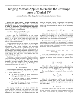
Gilmar Rosa et al.
Geociências
A note on robust and non-robust
variogram estimators
(Uma discussão sobre os estimadores robustos e
não-robustos de variogramas)
Sueli Aparecida Mingoti
Ph.D em Estatística. Professora Associada do Departamento de Estatística da
Universidade Federal de Minas Gerais-UFMG, Belo Horizonte, Minas Gerais
E-mail: [email protected]
Gilmar Rosa
Mestre em Estatística. Doutorando em Computação Aplicada
Instituto Nacional de Pesquisas Espaciais - INPE, São José dos Campos, São Paulo
E-mail: [email protected]
Resumo
Abstract
Em 1998, Genton propôs, um estimador de
variograma que seria robusto em relação à presença de
valores discrepantes (outliers) e o comparou com os
estimadores propostos por Matheron e Cressie-Hawkins.
Lark (2000) estendeu os resultados, avaliando o
desempenho dos estimadores na presença de nãonormalidade. Entretanto, ambos os trabalhos trataram
apenas do modelo de variograma esférico e com algumas
limitações. Nesse artigo, quatro estimadores de
variogramas, incluindo o de Genton, são comparados
através de simulação de Monte Carlo. Dados sem e com
outliers foram simulados, considerando os modelos de
variograma esférico, exponencial e senoidal. Os resultados
mostraram que os estimadores de Genton e o da Mediana
são melhores para dados com outliers, enquanto que o
de Matheron e o de Hastlett são melhores para dados
sem outliers, sendo o último adequado apenas para o
caso de análise de séries temporais.
In 1998 Genton proposed a variogram estimator
claimed to be robust against outliers and compared it
to Matheron’s and Cressie-Hawkins’ variogram
estimators. Lark (2000) extended the comparison
evaluating the effects of nonnormality. However, the
comparison was limited to the spherical variogram
model. In this paper 4 variogram estimators are
compared including Genton’s by using Monte Carlo
simulation. Data with and without outliers were
simulated using the spherical, exponential and wave
models. The results showed that Genton’s and the Median
estimators were the best choices for contaminated data,
while those of Matheron and Haslett presented better
results for non-contaminated date; this latter being
appropriate only for time series analysis.
Keywords: Spatial statistics, robust and non-robust
variogram estimators, outliers.
Palavras-chave: Estatística espacial, estimadores
robustos e não-robustos de variogramas, dados
discrepantes.
REM: R. Esc. Minas, Ouro Preto, 61(1): 87-95, jan. mar. 2008
87
A note on robust and non-robust variogram estimators
1. Introduction
Variogram is an important tool in
Geostatistics because it is used in the
kriging procedure (Marchant and Lark,
2004). Many variogram estimators can
be found in literature using parametric and
non-parametric methodologies (Chilès
and Delfiner, 1999). The better known is
Matheron’s (1962) which is very affected
by the presence of outliers in the data
set. Other alternatives are: Cressie and
Hawkins’ (1980) which was build to be
robust
against
outliers
and
nonnormality; Median’s (Cressie, 1993)
and Genton’s (1998) which were
supposed to be robust against outliers;
and the estimator proposed by Haslett
(1997) used in a time series context
especially for non-stationary data.
Genton (1998) showed that his estimator
had good performance in comparison to
that of Matheron’s and Cressie &
Hawkins’. However, only spherical
variogram models were considered in his
study and only one replicate was
generated for each simulated model. In
2000, Genton’s comparison was extended
by Lark (2000) who included Dowd’s
variogram estimator in his study and
showed that all the estimators, except
Matheron’s, were very affected by
nonnormality. Both mentioned papers
used only the spherical variogram model.
In this paper, the authors extended
Genton’s and Lark’s results in respect to
the outliers problem for non-spherical
model and explored the wave variogram
model, which has not appeared very
often in other published studies. The
Hastlett´s (1997) variogram estimator was
also included in the study.
2. Methods and materials
2.1 Geostatistics
methodolody
Geostatistics methodology was
initially formulated for geological data
(Matheron,1962). Nowdays, it has been
used in many other fields, even for
variables that are not of the physicalchemistry nature (Cressie, 1993; Mingoti
88
et. al, 2006). Let {Z(x), x ∈ D} be the spatial intrinsically stationary stochastic
process, i.e.
(i) E [Z(x)] = µ , ∀ x ∈ D
(ii) Var [Z(xl) - Z (xk)] = 2γ (xl - xk) , where xl ≠ xk ∈ D.
The quantities 2γ (.) and (.) are called, respectively, variogram and semivariogram
of the process {Z(x), x ∈ D}, where D is the domain under investigation. When the
variogram is only a function of the distance between the two coordinates, ||xl - xk||=h,
the process is also called isotropic. The variogram determines the weights given to
each sample value in the prediction of unsampled locations and it is also used to
estimate the kriging variance.
2.2 Variogram estimators
In this section, we briefly present the variogram estimators, so-called sample or
experimental variograms, which will be compared in this paper. We use the
conventional notation for Geostatistics methodology. For all the estimators, Nh, is
the cardinality of N(h) = {(xi, xj):||xi - xj)||=h} and {Z(x1), Z(x2),...,Z(xn)}is a sample of
the spatial process {Z(x), x ∈D}.
2.2.1 Matheron’s classical variogram estimator
The estimator based on the method-of-moments proposed by Matheron (1962)
is defined in (1) and is unbiased for the true theoretical values. It is the average of
the squared differences between observations separated by the distance h.
(1)
This estimator is very affected by the presence of outliers and even a single
discrepant datum can distort the final variogram estimates.
2.2.2 Cressie-hawkins robust variogram estimator
The estimator proposed by Cressie and Hawkins (1980) is given by
(2)
where
is a correction factor for bias when the variable
Z(.) is normal. This estimator was built to be robust against outliers and nonnormality
for distributions that are normal-like in the central region but heavier than normal in
the tails.
2.2.3 Median variogram estimator
The median variogram estimator (Cressie and Hawkins, 1980) is defined as
REM: R. Esc. Minas, Ouro Preto, 61(1): 87-95, jan. mar. 2008
(3)
Gilmar Rosa et al.
where med(.) denotes the median and Bh is a correction factor for bias when the
variable Z(.) is normal. Asymptotically Bh=0.457. This estimator is also known as
Dowd’s (1984) and it is supposed to be robust against outliers.
ARMA(p,q) stationary process then the
theoretical variogram of Z(.) can be
expressed as
2γ (h;θ) = 2σ² (1 - ρh)
2.2.4 Genton’s highly robust variogram estimator
The estimator proposed by Genton (1998) is defined as:
(4)
where
,
is the kth order statistics of the differences (Vi(h) - Vj(h)) and [w] is
the integer part of w. The factor 2.2191 is a correction for bias when Z(.) has a normal
distribution. Genton’s estimator is based on Rousseeuw and Croux (1993)
methodology. It is claimed to be highly robust against outliers.
2.2.5 Haslett’s variogram estimator
The variogram proposed by Haslett (1997) in the univariate time series context
is defined as:
(5)
where dhi = (Z(xi) - Z(xj)). Haslett’s estimator is the sample variance of the differences
(Z(xi) - Z(xj))and it was proposed as a tool to recognize ARMA stochastic processes
in time series context. In his paper Haslett showed that his estimator had a good
performance for non-stationary series.
2.3 Monte Carlo Simulation
In order to compare the performance of the variogram estimators, 100 samples
of size n=100 were simulated from each of the theoretical variograms presented in
Figure 1. Basically, the data were generated according to the methodology proposed
by Sharp (1982). The idea is to represent the semivariogram model in terms of an
ARMA (p,q) stationary process (Box and Jenkins, 1976). If Z(x), x∈ℜ, follows an
(a) - Spherical
(b) - Exponential
(6)
where σ² is the variance of the process,
ρh is the autocorrelation between Z(x)
and Z(x+h), and θ is the parameter vector
of the theoretical variogram of the
process. By using the relation (6) and
changing the values of (p,q), it is
possible to generate variogram models
such as spherical, exponential and wave.
For p=1 and q=0 the related variogram is
the spherical. For p=1 and q=1 the
exponential variogram is generated and
finally for p=q=1 the related variogram is
the wave. For all ARMA processes
considered in this paper the random noise
was generated according to a normal
distribution with zero mean and fixed
variance. All generated series have the
same mean value. Data with and without
outliers were simulated. The percentage
of outlier contamination were 5,10 and
15%. The introduction of outliers was
performed in three steps: (1) first a sample
was simulated from the respective
ARMA process without outliers, i.e,
Z(x)=δ+φZ(x-1)-αe(x-1)+ e(x), with e(.)
being the random error generated from a
normal distribution; (2) then a second
sample was simulated from the same
ARMA model but with a constant added,
i.e, Z(x)=δ+φ Z(x-1)-αe(x-1) + e(x) + δ* ;
(3) a percentual of the first sample was
then substituted for values from a
second sample. By using this procedure,
it was assured that the theoretical
covariance and correlation structure from
both ARMA models (generating data
with and without outliers) were the same.
(c) - Wave
Figure 1 - Simulated theoretical variogram models.
REM: R. Esc. Minas, Ouro Preto, 61(1): 87-95, jan. mar. 2008
89
A note on robust and non-robust variogram estimators
All the variogram estimators were
calculated for each generated sample for
n
n
h={1,2,…, [ ] }. The value [ ] was
2
2
chosen according to Journel and
Huijbregts’ rule (1997). For each value of
h the estimated and the theoretical
variogram values were compared by
using the mean, the absolute, the relative
and the squared mean errors. For each
estimator, the average of the variogram
estimates for each lag was calculated.
They are presented in Figures 2 to 4 with
the squared root of the square mean error
(SME) values. In each graph the
simulated variogram model is
represented by a solid line. All mean
errors presented a geometrical form
similar to the squared root of the SME
and will not be shown in this paper. The
square mean error (SME) values for each
variogram estimator are presented in
Tables 1 and 2, for the first 4 lags, for
data with and without outliers.
theoretical variogram model of the spatial
process. However, for larger h, the errors
increased significantly especially for
3. Results and
discussion
estimators for the wave variogram were
Matheron’s followed by Haslett’s,
Cressie & Hawkins’ and Genton’s.
Median presented the worst results. For
the spherical and exponential variogram
models having 5, 10 and 15% of outliers,
the Median estimator presented the best
performance, followed by Genton’s and
Cressie & Hawkins’. Haslett’s and
Matheron’s had the worse results. In
general, for small and larger lags and
regardless of the estimators used, the
insertion of a larger amount of outliers in
the data increased the value of the
variogram estimates and the number of
n
values of h near to [ ] . The best
2
For data with no outliers, the
analysis of the results showed that for
the spherical and exponential variogram
models, Haslett’s estimator achieved the
best performance followed by
Matheron’s, Genton’s and Cressie &
Hawkins’. The Median estimator
presented the highest number of errors
and greatest dispersion. In the case of
the wave variogram, for the initial lag h,
all the estimators were able to recover
the general mathematical form of the
Table 1 - Square Root of the Square Error Mean - Data without outliers.
Spherical Variogram
Lag(h)
Matheron
Cressie-H
Genton
Median
Haslett
1
0.8034
0.9935
10.503
14.089
0.8227
2
19.634
22.847
27.761
30.901
20.129
3
33.191
39.047
41.226
50.996
33.983
4
46.550
54.796
65.026
68.990
47.663
Exponential Variogram
1
35.912
36.797
33.997
37.970
35.431
2
24.040
26.932
32.882
32.881
24.646
3
59.628
62.213
67.707
72.892
61.130
4
93.087
95.355
111.677
113.774
94.964
Wave Variogram
90
1
26.658
41.787
43.520
72.689
26.830
2
97.376
164.102
198.830
266.239
98.185
3
188.116
331.809
343.898
555.262
189.798
4
265.146
511.283
604.818
887.817
267.636
REM: R. Esc. Minas, Ouro Preto, 61(1): 87-95, jan. mar. 2008
Gilmar Rosa et al.
Figure 2 - Performance results for variogram estimators - spherical model.
REM: R. Esc. Minas, Ouro Preto, 61(1): 87-95, jan. mar. 2008
91
A note on robust and non-robust variogram estimators
Figure 3 - Performance results for variogram estimators - exponential model.
92
REM: R. Esc. Minas, Ouro Preto, 61(1): 87-95, jan. mar. 2008
Gilmar Rosa et al.
Figure 4 - Performance results for variogram estimators - wave.
REM: R. Esc. Minas, Ouro Preto, 61(1): 87-95, jan. mar. 2008
93
A note on robust and non-robust variogram estimators
Table 2 - Square Root of the Square Error Mean- Data with outliers.
94
Lag(h)
1
2
3
4
Matheron
654.445
653.371
654.517
671.959
1
2
3
4
1.085.309
1.078.840
1.048.934
1.076.420
1
2
3
4
1.563.961
1.548.231
1.516.532
1.520.011
1
2
3
4
656.070
713.765
734.944
747.219
1
2
3
4
1.152.196
1.143.526
1.166.803
1.176.336
1
2
3
4
1.447.039
1.515.220
1.505.296
1.523.626
1
2
3
4
1.554.921
1.465.806
1.372.436
1.287.531
1
2
3
4
2.469.558
2.381.877
2.160.840
2.047.295
1
2
3
4
3.173.478
2.949.795
2.796.696
2.523.909
Spherical Variogram - 5% outliers
Cressie-H
Genton
92.983
33.770
137.552
78.191
178.439
109.140
215.220
156.547
Spherical Variogram - 10% outliers
239.243
83.459
318.031
176.450
372.010
236.223
433.446
331.939
Spherical Variogram - 15% outliers
456.329
149.521
567.293
295.837
653.019
392.787
705.257
509.807
Exponential Variogram - 5% outliers
65.617
14.249
174.251
109.808
262.287
186.249
315.131
268.705
Exponential Variogram - 10% outliers
217.412
51.002
351.862
206.261
458.268
315.021
541.807
447.674
Exponential Variogram - 15% outliers
383.122
110.299
615.008
373.650
722.597
512.435
828.245
710.080
Wave Variogram - 5% outliers
352.822
191.793
735.577
732.720
1.069.226
1.144.364
1.347.030
1.663.621
Wave Variogram - 10% outliers
755.574
414.729
1.332.707
1.351.223
1.749.147
1.874.147
2.128.884
2.550.874
Wave Variogram - 15% outliers
1.254.706
772.100
1.956.174
2.122.154
2.538.375
2.844.294
2.852.847
3.309.492
REM: R. Esc. Minas, Ouro Preto, 61(1): 87-95, jan. mar. 2008
Median
20.120
48.475
74.404
101.247
Haslett
661.554
660.820
662.282
680.150
43.988
91.820
134.933
181.427
1.140.997
1.149.541
1.106.994
1.143.266
68.490
139.458
200.122
247.440
1.580.291
1.564.785
1.532.945
1.536.659
23.514
67.798
139.898
196.350
663.533
722.099
743.573
755.985
21.652
103.604
194.810
271.093
1.167.444
1.159.428
1.181.755
1.192.505
35.470
177.080
283.309
393.094
1.462.512
1.531.612
1.521.783
1.540.404
139.841
534.613
1.096.379
1.678.248
1.573.291
1.490.297
1.405.224
1.328.201
228.535
787.117
1.499.643
2.374.310
2.497.187
2.415.639
2.201.810
2.096.445
401.619
1.350.985
2.481.067
3.385.333
3.208.233
2.989.318
2.844.066
2.578.106
Gilmar Rosa et al.
estimates errors. For contaminated data
all the robust estimators were able to
recover the geometric form of the
spherical, exponential and wave
theoretical variograms. Matheron’s and
Haslett’s estimators were only able to
recover the geometrical form of the wave
model. The estimators in the robust class
presented better results for the wave
variogram in the initial lags in
comparison to the non-robust ones. The
simulations also show that in general the
variogram estimators overestimate the
true values of the theoretical variograms.
These results were similar to those
observed in Genton’ paper (1998) for the
spherical model. In relation to the Journel
and Huijbregts’ rule (1997), Matheron,
Cressie-Hawkins and Genton’s
estimators presented more stable values
n
around the reference number [ ] ,
2
contrary to the Median estimator, which
was very unstable in this neighborhood,
and to the Haslett’s one,which had the
tendency to degenerate before the value
[ n ] . Since in general the sample variogram
2
n
values for h=1,2,…, [ ] are used to fit
2
the parameters of the true spatial model,
the results presented in this paper are
important because they show that
Journel and Huijbregts’ rule was not
suitable for Haslett’s and Median
estimators.
4. Conclusions
The results showed that in the presence of outliers, Genton’s and Median
variogram estimators should be preferred for the estimation of all the theoretical
variogram models presented in this paper. For data without outliers, Matheron’s and
Haslett’s had better performance except for the wave variogram model. Therefore, a
previous analysis for the presence of outliers in the data set is crucial in order to
decide which variogram estimator is more appropriate. The Journel and Huijbregts’
rule (1997) did not work very well for the Haslett’s and Median estimators.
5. Acknowledgements
The authors are thankful to CAPES and CNPq for financial support.
6. References
BOX, G., E., P.JENKINS, G., M. Time series analysis: forecasting and control. San Francisco:
Holden Day, 1976. 575 p.
CHILÈ, J-P.DELFINER, P. Geostatistics: modeling spatial uncertainty. New York: John
Wiley, 1999. 695 p.
CRESSIE, N. Statistics for spatial data. New York: John Wiley, 1993. 900 p.
CRESSIE, N., HAWKINS, M. Robust estimation of the variogram I. Mathematical Geology,
v. 12, n.2, p.115-125,1980.
GENTON, M. G. Highly robust variogram estimation. Mathematical Geology,v. 30, n.2,
p.213-221, 1998.
HASLETT, J. On the sample variogram and the sample autocovariance for non-stationary
time series. The Statistician, n. 46, p.475-485, 1997.
LARK, R.M. A comparison of some robust estimators of the variogram for use in soil survey.
European Journal of Soil Sciences, n.51, p. 137-157, 2000.
JOURNEL, A. G., HUIJBREGTS, Ch.J. Mining geostatistics. London: Academic Press,
1978. 600 p.
MARCHANT, B. P., LARK, R. M. Estimating variogram uncertainty. Mathematical
Geology, v.36, n. 8, p. 868-898, 2004.
MATHERON, G. Traité de géostatistique appliquée, Tome I. Mémoires du bureau de
recherches géologiques et minières principles. Paris: Editions Technip, 1962. n. 14.
333p.
MINGOTI, S., GUIMARÃES, A. L., ROSA, G. Describing the total number of diagnosed
cases of aids by means of geostatistics. Revista de Matemática e Estatística, v. 24, n.1,
p.61-76, 2006.
ROUSSEEUW, P. J., CROUX. C. Alternatives of the median absolute deviation. Journal of
American Statistics Association, v. 88, n. 424, p.1273-1283, 1993.
SHARP, W. E. Stochastic simulation of semivariogram. Mathematical Geology, v.14, n.5,
p.445-457, 1982.
Artigo recebido em 26/02/2007 e aprovado em 27/07/2007.
REM - Revista Escola de Minas
72 anos divulgando CIÊNCIA.
******
www.rem.com.br
REM: R. Esc. Minas, Ouro Preto, 61(1): 87-95, jan. mar. 2008
95