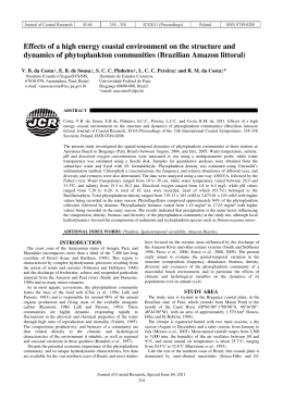
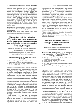
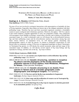
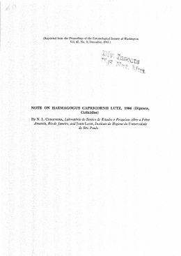
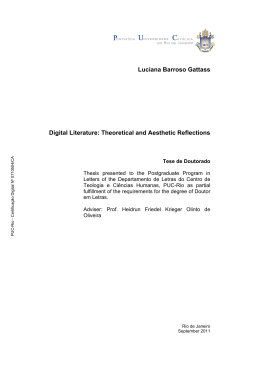
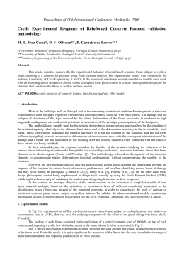
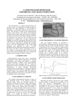
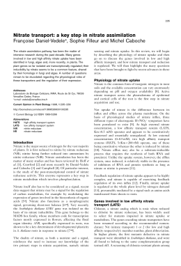
Deep-Sea Research I 46 (1999) 597 — 636
A physical—biochemical model of plankton
productivity and nitrogen cycling in the Black Sea
Temel Oguz *, Hugh W. Ducklow, Paola Malanotte-Rizzoli,
James W. Murray, E.A. Shushkina, V.I. Vedernikov,
Umit Unluata
Institute of Marine Sciences, Middle East Technical University, Erdemli, Icel, Turkey
The College of William and Mary, Virginia Institute of Marine Sciences, Gloucester Point, VA, USA
Department of Earth, Atmospheric and Planetary Sciences, Massachusettes Institute of Technology,
Cambridge, MA, USA
School of Oceanography, University of Washington, Box 357940, Seattle, WA, USA
P.P. Shirshov Institute of Oceanology, Russian Academy of Sciences, Moscow, Russia
Received: 8 July 1997; received in revised form 10 February 1998; accepted: 27 March 1998
Abstract
A one-dimensional, vertically resolved, physical—biochemical upper ocean model is utilized
to study plankton productivity and nitrogen cycling in the central Black Sea region characterized by cyclonic gyral circulation. The model is an extension of the one given by Oguz et al.
(1996, J. Geophys. Res. 101, 16585—16599) with identical physical characteristics but incorporating a multi-component plankton structure in its biological module. Phytoplankton are
represented by two groups, typifying diatoms and flagellates. Zooplankton are also separated
into two groups: microzooplankton (nominally (200 lm) and mesozooplankton (0.2—2 mm).
The other components of the biochemical model are detritus and nitrogen in the forms of
nitrate and ammonium. The model incorporates, in addition to plankton productivity and
organic matter generation, nitrogen remineralization (ammonification) and ammonium oxidation (nitrification) in the water column. Numerical simulations are described and compared
with the available data from the central Black Sea. The main seasonal and vertical characteristics of phytoplankton and nutrient dynamics inferred from observations appear to be
reasonably well represented by the model. Fractionation of the biotic community structure is
shown to lead to increased plankton productivity during the summer period following the
diatom-based early spring (March) bloom. The annual nitrogen budget for the euphotic zone
reveals the substantial role of recycled nitrogen in the surface waters of the Black Sea. 1999
Elsevier Science Ltd. All rights reserved.
* Corresponding author. Tel.: 90 324 521 2406; fax: 90 324 521 2327; e-mail: [email protected]
0967-0637/99/$ — see front matter 1999 Elsevier Science Ltd. All rights reserved.
PII: S 0 9 6 7 - 0 6 3 7 ( 9 8 ) 0 0 0 7 4 - 0
598
T. Oguz et al. / Deep-Sea Research I 46 (1999) 597 — 636
1. Introduction
The Black Sea is known as one of the best examples of highly stratified marginal
seas. This two layer stratified system is accompanied by a distinct biochemical
structure characterized by complete anoxia of the sub-pycnocline waters and their
separation from the oxygenated surface waters through a transition zone, called the
Suboxic Layer (SOL) (Murray et al., 1989). The oxygenated surface layer comprises an
euphotic zone of about 40—50 m underlain by an oxycline/nutricline zone of 20—30 m.
The suboxic layer has a thickness of about 20—40 m and contains no measurable
oxygen or sulphide.
The Black Sea contains an efficient mechanism of nitrogen cycling. About 90% of
the particulate organic material sinking from the euphotic zone is mineralized in the
euphotic zone and oxycline/nutricline zone below. The nutrients regenerated are then
resupplied back to the surface waters, where they are depleted eventually by biological
utilization (e.g. spring phytoplankton bloom). Only a small fraction of the particulate
matter sinks to the deeper, anoxic zone (Lebedeva and Vostokov, 1984; Karl and
Knauer, 1991). In the anoxic layer, particulate flux may give rise to chemosynthetic
production, which amounts to approximately 10% of the photosynthetic production
(Deuser, 1971; Brewer and Murray, 1973). As compared with basins rich in oxygen,
a distinguishing feature of the Black Sea is limitation of primary production by
subsurface nitrogen supply due to extensive nitrate consumption by denitrification in
the subsurface waters. The deep anoxic water in the Black Sea contains no measurable
nitrate but constitutes a large pool of reduced nitrogen in the forms of ammonium and
dissolved organic nitrogen. The existing data indicate that ammonium transported
upwards is oxidized immediately near the suboxic-anoxic interface zone by nitrate
and MnO (Murray et al., 1997) and lost to the atmosphere in the form of nitrogen
gas. The anoxic layer thus does not appear to be a source of dissolved inorganic
nitrate to the euphotic zone in the Black Sea.
The Black Sea has a major diatom bloom during March (Sorokin, 1983; Vinogradov, 1992; Vedernikov and Demidov, 1993). A second bloom occurs sometime
during autumn. Two or more additional phytoplankton peaks, mainly of coccolithophorids and flagellates, are usually observed during late spring and summer
(Bologa, 1986). Emiliania huxleyi blooms occurring in the months of June and July are
evident in the CZCS imagery (Sur et al., 1996).
The early spring bloom is the most robust feature of the yearly phytoplankton
structure and is present in every data set (see Koblentz-Mishke, 1970; Sorokin, 1983;
Lebedeva and Vostokov, 1984; Vedernikov and Demidov, 1993). Formation and
timing of summer blooms, on the other hand, seem to be much more sensitive to local
conditions and exhibit considerable regional and interannual variability (Vinogradov,
1992; Vedernikov and Demidov, 1993; Sur et al., 1996).
As a part of our ongoing interdisciplinary modeling efforts, we recently constructed
a one-dimensional nitrogen-based, vertically resolved, coupled physical—biological
model of the lower trophic level to examine the first order physical and biological
processes controlling the seasonal cycle of the plankton productivity in the surface
waters of the Black Sea (Oguz et al., 1996, 1997). The biological part of the model was
T. Oguz et al. / Deep-Sea Research I 46 (1999) 597 — 636
599
kept quite simple, including only single phytoplankton and herbivore zooplankton
groups (1P1Z), detritus, nitrate and ammonium, which form the ‘‘minimum critical
set’’ (GLOBEC, 1995). The model was applied for conditions appropriate to the
central Black Sea, which possesses simpler ecosystem behavior than do the highly
complex western shelf and Rim Current frontal zones. This model had a reasonable
success in reproducing monthly variations of the upper layer water column stratification characteristics. It demonstrated the crucial role of mixed layer dynamics during
convective overturning events, which are missing in most ecosystem models. The
biological component of this coupled model was able to simulate the spring and fall
blooms and the summer subsurface chlorophyll maximum layer. This simple model
was useful for examining the basic physical and biological processes controlling the
seasonal cycle of plankton productivity in the Black Sea.
One drawback of the simplified 1P1Z ecosystem model was underestimation of
the summer production. The summer subsurface chlorophyll concentrations were
found to be somewhat lower than observed values. The limited capability of 1P1Z
models in predicting summer chlorophyll values was noted earlier by Sarmiento et al.
(1993) in their North Atlantic model. Armstrong (1994) pointed out that multiple
prey—multiple predator models can alleviate the limitations imposed by 1P1Z approaches and, as in the North Atlantic case, may generate increased chlorophyll
concentrations comparable with observations. In the present paper, we introduce two
phytoplankton species groups, typifying diatoms and flagellates, and two zooplankton groups (micro- and mesozooplankton). Then we show how this slightly more
complex representation of plankton food web structure leads to enhanced production
during late spring and summer in the Black Sea model. In view of growing recognition
of its importance, we also include a simple representation of ammonium oxidation
(nitrification).
In more general terms our objective, given the idealized external conditions and
idealized trophic-dynamic description of the system, is to investigate how successfully
we can simulate the main features of nitrogen cycling and the yearly evolution of
plankton production in the central Black Sea.
2. Model description
The model consists of physical and biochemical modules connected through the
Mellor-Yamada level 2.5 turbulence module used for calculating vertical eddy fluxes.
The details of the physical and turbulent components of the coupled model have been
described previously (Oguz et al., 1996). We therefore present here only the basic
elements of the biochemical model, whose main features generally follow Ducklow
and Fasham (1992), excluding bacterial processes.
2.1. Governing equations
Nitrogen cycling and plankton dynamics in the upper layer of the Black Sea
are modeled using two groups of phytoplankton and of herbivorous/omnivorous
600
T. Oguz et al. / Deep-Sea Research I 46 (1999) 597 — 636
zooplankton, together with labile particulate detritus D, nitrate NO and ammonium
NH . The two phytoplankton groups typify diatoms and flagellates, and the two
herbivore groups are microzooplankton Z (nominally(200 lm) and mesozooplan
kton Zl (0.2—2 mm). The microzooplankton compartment includes heterotrophic
flagellates, ciliates and juvenile copepods. The mesozooplankton compartment essentially represents adult copepods. Particulate organic detritus is assumed to be converted directly to ammonium without explicitely considering the microbial loop
mediating the particle decomposition process.
The local temporal variations of all biological variables are expressed by equations
of the general form
*F
*F
*
*F
#w
"
(K #l )
#R
*z *z
*z
$
*t
(1)
where t is time, z is the vertical coordinate, * denotes partial differentiation,
w signifies the sinking velocity, K is the vertical turbulent diffusion coefficient, and
l is its background value. Here, we consider downward sinking only of detrital
material; w is thus set to zero except in the detritus equation. The interaction term,
R , is expressed as a balance of biological sources and sinks for each of the variables
$
described below. A schematic representation of the biological processes included in
the model is shown in Fig. 1a.
2.1.1. Phytoplankton
Variations of diatom (P ) and flagellate (P ) stocks are governed by a balance
between growth (primary production) and losses due to herbivore grazing and
physiological mortality. The effects of respiration and phytoplankton excretion are
included in the latter loss term, since our model does not include a microbial loop
component at present.
Flagellates: R "p UP !G (P ) Z !Gl (P )Zl!m P
.
(2)
Diatoms: R "p UP !G (P ) Z !Gl (P ) Zl!m P
.
(3)
The phytoplankton growth is modeled as the product of the maximum specific growth
rate p, the overall limitation function U and the phytoplankton concentration P. The
overall limiting factor on the maximum growth rate is defined as the minimum of the
light and nutrient limitation terms:
U"min[a(I), b (NO , NH )]
(4)
where a(I) is the light limitation function, b (NO , NH ) is the sum of ammonium and
nitrate limitation functions represented, respectively, by b (NH ) and b (NO ). They
are expressed by standard Michaelis—Menten uptake formulations (see Oguz et al.,
1996). For simplicity, we ignore the difference in the photosynthetic and nutrient
uptake abilities of diatoms and flagellates. The temperature control on the phytoplankton growth is also neglected. This is justified in the Black Sea by the fact that both
T. Oguz et al. / Deep-Sea Research I 46 (1999) 597 — 636
601
Fig. 1. (a) A schematic diagram showing the biological processes and interactions included in the model.
(b) The trophic interactions between different plankton groups and food preference coefficients considered
in the model.
early spring (typically in March) surface bloom and summer subsurface production
below the seasonal thermocline occur at fairly uniform water temperatures around
7—10°C. We also exclude the role of silicate on the diatom blooms. Nitrate has been
considered here as the single limiting nutrient for the central Black Sea conditions.
The light limitation is parameterized according to Jassby and Platt (1976) by
a(I)"tanh[aI(z, t)]
(5)
I(z, t)"I exp[!(k #k P) z]
(6)
where a denotes the photosynthetic quantum efficiency parameter controlling the
slope of a(I) versus the irradiance curve at low values of the photosynthetically active
irradiance (PAR). I denotes the surface intensity of the PAR, taken as half of the
climatological incoming solar radiation from the data given in Table 2 in Oguz et al.
(1996). k is the extinction coefficient of the sea water, and k is the phytoplankton
602
T. Oguz et al. / Deep-Sea Research I 46 (1999) 597 — 636
self-shading coefficient. In the above formulation, both of these light attenuation
coefficients are taken to be constant with depth.
2.1.2. Zooplankton
Changes in the microzooplankton (Z ) and mesozooplankton (Zl) biomasses are
controlled by ingestion, grazing, mortality and excretion.
Microzooplankton: R "c [G (P )#G (P )]Z !Gl (Z )Zl!k Z !j Z (7)
Q 8
Mesozooplankton: R l"cl [Gl (P )#Gl (P )#Gl (Z )]Zl!kl Zl!j Zl
(8)
8
J
where kl and k are excretion rates, jl and j are mortality rates, and cl and c are the
assimilation coefficients. In Eqs. (7) and (8), the mortality terms are expressed in the
quadratic form as suggested by Steele and Henderson (1992). The role of other
functional forms of the mortality (e.g. linear, hyperbolic) on the annual plankton
variations are also investigated in this paper (see Section 4.8). Grazing is represented
by the Michaelis—Menten relation and considers the food preferences, diatoms vs
flagellates, of the two zooplankton groups. Using measures of zooplankton food
preferences shown in Fig. 1b, we define total food available for each zooplankton
group as
F "b P #b P and Fl"a P #a P #a Z .
(9)
The grazing rates of micro and mesozooplankton on flagellates are then defined by
aP
bP
.
and Gl (P )"r l
G (P )"r
R #Fl
R #F
Similarly, the grazing rates of the two zooplankton groups on diatoms are
(10)
bP
aP
G (P )"r
and Gl (P )"r l (11)
R #F
R #Fl
and a similar expression is applied for the grazing of mesozooplankton on the
microzooplankton group. In Eqs. (10) and (11), r and r l denote the maximum
specific grazing rates, and R is the half saturation ratio. As may be noted from Eqs. (7)
and (8), zooplankton groups are assumed to assimilate uniform, constant fractions
(represented by cl and c ) of their ingestion.
Fasham et al. (1990) argued that the coefficients of food preferences should be
expressed as functions of the relative prey densities (see Appendix A in Fasham et al.,
1990). This approach seems to be more plausible than our specification of constant
coefficients above, but it may introduce an additional complexity to the model due to
the depth and time dependence of the coefficients. This point will be further discussed
in Section 4.7.
2.1.3. Detritus
Fecal pellets, constituting the unassimilated part of ingested food, and phytoplankton and zooplankton mortalities, are the sources of detritus. As the detrital material
T. Oguz et al. / Deep-Sea Research I 46 (1999) 597 — 636
603
sinks with a speed w , it is transformed into ammonium with a rate eD. Here, for
simplicity, the model considers only one class of detritus, which is produced by both
phytoplankton and zooplankton groups, and sinks with a single settling velocity w .
A more realistic approach would be to consider different size classes of detritus
produced separately from different plankton groups and sinking with different settling
velocities (cf. Prunet et al., 1996).
R "(1!c ) [G (P )#G (P )] Z #(1!cl) [Gl (P )#Gl (P )#Gl(Z )]Zl
"
#m P #m P #j Z#jlZl !eD.
(12)
2.1.4. Nutrients
Two forms of nitrogen (ammonium and nitrate) support phytoplankton growth. As
we shall discuss in Section 4, however, their roles in supporting regenerated and new
production are not distinct, since the model includes nitrification. Excretion by two
zooplankton groups and remineralization of detritus supply recycled ammonium. The
losses are ammonium uptake during phytoplankton production and its oxidation to
nitrate. The intermediate step of nitrite production was included in the nitrification
process in our preliminary experiments but taken out later, since it had no distinguishable contribution to the euphotic zone budget. The data (cf. Codispoti et al., 1991;
Basturk et al., 1994) indicate that nitrite concentrations in the euphotic zone are
always smaller than those of other forms of nitrogen.
b
(p P #p P )!X (z)NH #eD#k Z #klZl .
Ammonium: R "!U
,&
b
(13)
The nitrate equation consists of a source from ammonium oxidation and a loss by
nitrate uptake, which also includes the ammonium inhibition effect (Oguz et al., 1996).
b
Nitrate: R "!U (p P #p P )#X (z) NH .
,-
b
(14)
2.2. Boundary conditions
All turbulent fluxes are set to zero at the surface and bottom boundaries of the
biochemical model. Thus, we take
*F
(K #l )
"0 at z"0 and z"!h .
*z
(15)
In addition, the detritus equation includes
w D"0 at z"0 and
*(w D)
"0 at z"!h .
*z
(16)
604
T. Oguz et al. / Deep-Sea Research I 46 (1999) 597 — 636
The bottom boundary of the model, h , is taken at a depth of 150 m, which is situated
well below the level of active remineralization and nitrification taking place in the
model. This choice of water column depth, together with the choice of a relatively low
settling speed of 2.0 m d\, implies that our detrital pool, formed essentially by small
particles, is remineralized completely within the water column without any export flux
of particulate matter from the system. We thus consider that larger particles with
much higher sinking rates are lost immediately and do not take part in the nitrogen
recycling process in the upper layer. As shown in Oguz et al. (1996) and reported by
similar models of plankton productivity (e.g. Jamart et al., 1977; Stigebrandt and
Wulff, 1987; Sarmiento et al., 1993; Loukos et al., 1997), the detritus sinking velocity is
in fact one of the critical model parameters, whose choice may considerably alter the
annual plankton structure.
Within the framework of a one dimensional model, the assumption of complete
remineralization is a fairly realistic approximation. The sediment trap observations
suggest remineralization of more than 90% of the particulate organic matter within
the upper layer (&100 m) of the Black Sea (Karl and Knauer, 1991). The advantage of
a 100% remineralization assumption is to have a fully conservative system (note that
R "0 in our model), which therefore does not require us to deal with nitrate-based
$
source/sink fluxes at the lower boundary of the model. In fact, specification of nitrate
flux at the lower boundary, to compensate the fecal pellet loss, is not a straight
forward issue in a one dimensional Black Sea ecosystem model. Contrary to the
presence of deep nitrate pools in the Atlantic or Pacific, Black Sea subsurface waters
consist of a deep ammonium pool, without any nitrate below about 100 m depth (see
Section 3.2). This implies that organic matter loss to the deep waters should therefore
be compensated by lateral nitrate fluxes, mostly originating from the Danube River
discharge. On the other hand, the deep ammonium pool does not act as a nitrogen
source to the euphotic zone in the Black Sea, because the ammonium transported
upwards is consumed by its oxidation near the oxic/anoxic interface (see Fig. 5d). In
reality, the bottom boundary of the euphotic zone is a very complicated region of
redox processes in the Black Sea. A key feature is the suboxic zone, where the total
fixed nitrogen goes to a strong minimum, suggesting conversion to nitrogen gas
(Murrary et al., 1999). Near the anoxic interface, ammonium is oxidized with MnO
and converted to nitrogen gas. These processes are too complicated to include in this
model and beyond the scope of the present work.
2.3. Initial conditions and numerical procedure
The physical model is initialized by stably stratified upper ocean temperature and
salinity profiles representative of the autumn conditions for the interior part of the sea.
It is forced by the monthly climatological wind stress and surface thermal fluxes (see
Table 2 in Oguz et al., 1996), whereas no-stress, no-heat and no-salt flux conditions
are specified at the bottom. The biochemical model is initialized by a vertically
uniform nitrate concentration of 4 mmol/m within the euphotic and nitracline
zones. The nitrate concentrations are set to zero below 75 m, corresponding roughly
to oxygen depleted waters of the central Black Sea. Other state variables of the
T. Oguz et al. / Deep-Sea Research I 46 (1999) 597 — 636
605
biochemical model are initialized with small constant values over the water column to
allow positive growth and utilization. Once the model equations are integrated ahead
in time, the internal dynamics (i.e. plankton productivity, nitrogen cycling and vertical
diffusion) establish realistic structures of the nitrate and other variables after a few
years of transient adjustment.
The details of the numerical solution procedure are described in Oguz et al. (1996).
A total of 50 vertical levels is used to resolve the 150 m thick water column. A time
step of 10 min is used in the numerical integration of the system of equations. First, the
physical model is integrated for five years to achieve a yearly cycle of the upper layer
physical structure. Using these results, the biochemical model is then integrated for
four years, which is sufficient to complete its transient adjustment from the initial
conditions.
3. Observations
3.1. Chlorophyll-a
A series of vertical profiles of chlorophyll-a concentrations is shown in Fig. 2. These
profiles are selected from measurements performed within the interior of the sea
during the past decade on eight different cruises by the Shirshov Institute of Oceanology, Moscow (Vedernikov and Demidov, 1993). The first four profiles of March 1988
provide a clear indication of the spring bloom during the first half of the month. The
profiles are homogeneous within the upper 40 m of the water column with typical
concentrations of 2 mg m\. The bloom declines gradually during the second half of
March to about 0.5 mg m\ at the end of the month. The April and May data reveal
surface mixed layer chlorophyll concentrations around 0.2—0.3 mg m\. A narrow
subsurface chlorophyll maximum may also be traced at some stations. The thickness
of this layer is less than 20 m, centered around 40 m. In May, peak concentrations do
not exceed 0.5 mg m\.
An increase in subsurface chlorophyll concentrations is observed during June.
The subsurface chlorophyll maximum reaches 1.0 mg m\ near the base of the
euphotic zone. The thickness and position of the subsurface maximum zone, however,
vary regionally within the basin. This kind of enhanced subsurface chlorophyll
signature seems to persist throughout the summer, as shown by the August 1989 data
set. The October 1978 data suggest that the late summer-early autumn is a period in
which the subsurface chlorophyll maximum layer is gradually eroded and narrowed.
As implied by the data sets, this transitional period is followed by initiation of an
autumn bloom episode towards the end of October. The November 1991 data set
exhibits similar autumn bloom formation during the first half of November, with
chlorophyll concentrations in excess of 1 mg m\ in the 25 m thick surface mixed
layer.
Interpretation of the chlorophyll data shown in Fig. 2 must consider interannual
and regional variations. These merged observations indicate two distinct surface
bloom episodes during March and November and increased subsurface production in
606
T. Oguz et al. / Deep-Sea Research I 46 (1999) 597 — 636
the summer months (June—August). Early October appears to be a transitional period
of weak chlorophyll concentrations prior to the autumn bloom.
3.2. Phytoplankton and zooplankton
The yearly variations of the euphotic zone-integrated phytoplankton and zooplankton (micro- and meso-) biomasses are shown in Fig. 3. These distributions are formed
using the data collected within the central Black Sea by the Shirshov Institute of
Oceanology during seven cruises between 1978 and 1992. Because they are composites
of different data sets, they can be used to infer only major signatures of the plankton
system.
As in the case of the chlorophyll (Fig. 2), the phytoplankton data (Fig. 3a) reveal
a strong bloom in early March, with the highest phytoplankton biomass of
&7.0 gC m\ measured during 1991 survey. The data exhibit a decreasing trend
Fig. 2. Annual variations of the vertical chlorophyll-a (mg m\) structure derived from measurements
carried out during 1978—1989 by Shirshov Institute of Oceanology, Moscow, and compiled by V.I.
Vedernikov. The dates are shown for each profile in the form of three consecuative two digit numbers
indicating the year, the month and the day of the measurements.
T. Oguz et al. / Deep-Sea Research I 46 (1999) 597 — 636
607
Fig. 2. (continued)
during late March—April, towards a minimum value of around 1.0 gC m\ at the end
of April. A secondary peak is observed in November, as inferred earlier from the
chlorophyll data. The summer data, limited to the August—September period, suggest
biomass values &2.0 gC m\.
608
T. Oguz et al. / Deep-Sea Research I 46 (1999) 597 — 636
Fig. 2. (continued)
The yearly mesozooplankton structure (Fig. 3b) follows generally that of the
phytoplankton. A major increase in the biomass occurs towards the end of
March—mid-April, following the strongest phytoplankton bloom of the year. The peak
biomass values are &2.0 gC m\ and reduced by half later during the summer.
Because no measurements are available in the second half of November and December, the data do not provide a clear indication of autumn—early winter biomass
increase following the autumn phytoplankton bloom. The microzooplankton, on the
other hand, do not exhibit any appreciable seasonal variations. Their biomass remains typically below 0.5 gC m\ throughout the year (Fig. 3c).
3.3. Nitrate
Examples of summer and winter nitrate profiles are shown in Fig. 4. The summer
profiles, which are taken within the cyclonic gyre of the western basin, exhibit
complete nitrate depletion within the upper 50 m, corresponding roughly to the
euphotic zone. Nitrate then increases sharply to a maximum value of 8 mmol m\ at
70—80 m through a sharp nitracline zone. It is quantified in the next section that
T. Oguz et al. / Deep-Sea Research I 46 (1999) 597 — 636
609
Fig. 3. A composite picture of the euphotic layer integrated (a) phytoplankton, (b) mesozooplankton, (c)
microzooplankton distributions (in mgC m\) within a year compiled from different data sources (open
hexagons, 1978; open stars, 1984; open triangles, 1988; solid circles, 1989, solid triangles and stars, 1991;
solid hexagons, 1992).
formation of the nitracline through a sharp nitracline zone is a consequence of intense
remineralization—nitrification processes.
The region below the nitrate peak is characterized by a sharp reduction in nitrate
concentrations. In this oxygen-deficient part of the water column, organic matter
degradation occurs via denitrification. In this process, bacteria utilize nitrate ions to
oxidize organic matter from the surface layer. The nitrate is then reduced to nitrogen
gas, with nitrite as an intermediate product. The nitrogen gas is eventually ventilated
to the atmosphere. Denitrification continues until all the nitrate is consumed within
the oxygen-deficient part of the water column. The lower limit of this zone coincides
roughly with the onset of the H S layer. These processes, however, have not been
included in the present work.
The winter nitrate profile reveals concentrations in excess of 2.0 mmol m\ within
the upper mixed layer of about 60 m. As we shall show in the next section, the
610
T. Oguz et al. / Deep-Sea Research I 46 (1999) 597 — 636
Fig. 4. Observed nitrate profiles in the upper water column of the Black Sea. Squares and circles signify the
measurements of the R.V. Knorr at the center of the western gyre on 9 June and 18 July 1988. Stars show
winter measurements performed at a station in the Rim Current frontal zone along the Turkish coast of the
western Black Sea on 18 January 1989.
convective overturning process associated with the winter cooling is responsible for
seasonal changes in the surface layer nitrate concentrations. The subsurface nitrate
maximum of the observed winter profile in Fig. 4 is located at deeper levels than it is in
the summer profiles. This is because this station is situated along the peripheral zone
of the circulation system, which has an anticyclonic character. To our knowledge,
winter nitrate measurements within the cyclonically dominated central basin are not
available.
3.4. Ammonium
The vertical ammonium structure shown in Fig. 5a is characterized by low concentrations of less than 0.5 mmol m\ within the upper 100 m of the water
column, where it is converted continually to nitrate by nitrification and utilized by
phytoplankton. The ammonium concentrations exhibit occasional peaks of about
0.5 mmol m\ within the euphotic zone. It is shown in the next section that these
peaks are related to summer phytoplankton production.
The ammonium concentration increases linearly below about 100 m depth, where
the nitrate vanishes and the H S layer begins (Fig. 5b). It attains typically a value of
10 mmol m\ at 150 m and 20 mmol m\ at about 200 m depth. The deep ammonium pool has accumulated as a result of organic matter decomposition by sulfate
T. Oguz et al. / Deep-Sea Research I 46 (1999) 597 — 636
611
Fig. 5. (a). Ammonium profiles for the upper water column from the R.V. Knorr measurements at the
center of the western gyre on 25 May and 29 June 1988. (b) Ammonium profiles from the R.V. Knorr
measurements at the center of the western gyre, showing ammonium variations within the anoxic layer on
9 June and 18 July 1988.
reduction within the last 5000 years, since the Black Sea was converted into a twolayered stratified system (Boudreau and Leblond, 1989). The gradient of the ammonium profiles in the vicinity of the oxic-anoxic interface implies that no ammonium
is supplied to the photic zone from the anoxic region.
As we have pointed out in the previous section, the present version of our Black Sea
biogeochemical model includes neither denitrification (which is responsible for the
formation of the lower nitracline) nor sulfate reduction (which leads to increases in the
NH concentrations in the anoxic layer). These simplifications are justifiable for our
purpose of investigating the more intensive surface processes of plankton productivity.
4. Numerical simulations
4.1. Specification of parameters
The definition of parameters and their values are given in Table 1. Some of them are
provided by existing observations and thus taken from the published literature on the
Black Sea. Others are chosen from other seas having similar pelagic ecosystem and
physical characteristics (see Oguz et al. 1996 for further discussion). The values of the
photosythesis quantum efficiency parameter a and the light extinction coefficient
k are taken from our recent light measurements (Vidal, 1995). Their optimum values
for the central Black Sea conditions are set to a"0.01(W m\)\ and k "0.08 m\.
The self shading coefficient k is set to 0.07 m(mmol N)\. Its value is, however,
612
T. Oguz et al. / Deep-Sea Research I 46 (1999) 597 — 636
Table 1
Model parameters used in the numerical experiments
Parameter
Definition
Value
a
k
k
p
p
m
m
r
J
r
b ,b
Photosynthesis efficiency parameter
Light extinction coefficient for PAR
Phytoplankton self-shading coefficient
Maximum growth rate for diatoms
Maximum growth rate for flagellates
Diatom mortality rate
Flagellate mortality rate
Mesozooplankton maximum grazing rate
Microzooplankton maximum grazing rate
Food preferences of microzooplankton on flagellates
and diatoms
Food preferences of mesozooplankton on flagellates,
diatoms and microzooplankton
Mortality rate for microzooplankton
Mortality rate for mesozooplankton
Zooplankton excretion rates
Assimilation efficiencies
Half-saturation constant in nitrate uptake
Half-saturation constant in ammonium uptake
Half-saturation constant for zooplankton grazing
Ammonium inhibition parameter of nitrate uptake
Detritus decomposition rate
Detrital sinkal rate
Nitrification rate
Background kinematic diffusivity for z)75 m
Background kinematic diffusivity for z'75 m
0.01 m W\
0.08 m\
0.07 m (mmol N)\
1.5 d\
1.0 d\
0.04 d\
0.08 d\
0.8 d\
1.2 d\
a ,a ,a
j
j,
k,k
c ,c
R
R
R
t
e
w
X
l
l
0.7, 0.2
0.3, 0.8, 0.7
0.04 d\
0.08 d\
0.07 d\
0.75
0.5 mmol N m\
0.2 mmol N m\
0.5 mmol N m\
3 (mmol N m\)\
0.1 d\
2.0 m d\
0.05 d\
1;10\ m s\
0.5;10\ m s\
found not to be critically important for altering the annual plankton distribution. The
values of the half saturation constants are chosen from the literature (e.g. Fasham et
al., 1990). They have typical values around 0.5 mmol N m\. For NO we use
R "0.5 and for NH , R "0.2. Our sensitivity experiments indicate that the model
response is not critically sensitive to their values.
The assimilation efficiencies (c , cl) are taken to be 0.75, which is the most com
monly cited value in the literature. The choices of the mortality and excretion rates
depend on processes that are represented by these terms, but their typical values cited
in the literature are around 0.05 d\. We use here phytoplankton mortality rates of
m "0.08 and m "0.04 d\. For zooplankton, we let the mortality rates be j "0.04
and jl"0.08 and the excretion rates (k , kl) 0.07 d\. Their particular choices are
found to have secondary effects on the simulations. The values of maximum growth
rates (p , p ) and of the maximum grazing rates (r , rl) are set to (1.0, 1.5) d\ and (1.2,
0.8) d\. In the model, each group of zooplankton can feed on two types of prey. We
assume that the microzooplankton prey with greater efficiency on flagellates than on
diatoms. We thus set the efficiency parameters to b "0.7 and b "0.2. Mesozooplan
kton are considered to prey more efficiently on diatoms (a "0.8) than on flagellates
T. Oguz et al. / Deep-Sea Research I 46 (1999) 597 — 636
613
(a "0.3). Their food preference for microzooplankton is set to a "0.7. These values
were suggested by observations carried out by Shirshov Institute of Oceanology,
Moscow, in the Black Sea.
The ammonium oxidation rate X is taken to be 0.05 d\ above the depth of the
15.8 kg m\ sigma-t level, which corresponds to the total oxygen depletion level in the
central Black Sea. This value of X is estimated from measurements of Ward and
Kilpatrick (1991). At deeper levels, where nitrification does not occur, its value is set to
zero. The choice of constant X above the depth of the 15.8 kg m\ sigma-t level is an
idealization of its more realistic depth dependent representation according to the
oxygen variations in the water column.
Within the euphotic layer and the nitracline, we assume a background vertical
diffusion of 10\ m s\. A smaller value of 0.5;10\ m s\ is used for the deeper
part of the water column, where there is no biological activity, and corresponds to the
permanent pycnocline with strong density differences (&3.0 kg m\) over an interval
of 50 m. Using the emprical expression given by Gargett (1984), Lewis and Landing
(1991) arrived at similar values of the vertical diffusivity in their Black Sea manganese
cycling model.
A series of simulation experiments was carried out to classify these parameters
according to sensitivity of major observed features to the choices of their values. In
this way, we try to identify the most critical parameters and their range of values for
predicting the annual cycle of plankton productivity consistent with available observations. Some examples of these sensitivity experiments will be described in the next
sections.
4.2. Mixed layer structure
In Oguz et al. (1996), we described in some detail the ability of our physical model to
simulate observed mixed layer temperature and salinity during the year using a fairly
sophisticated turbulence parameterization. It was shown that seasonal cycles were
correctly reproduced, with maximum sea surface temperature deviations of less than
0.5C, and maximum mixed layer depth differences of 10 m. Here, we present some
additional features of the mixed layer structure using depth-time distributions of the
temperature and vertical eddy diffusivity during a perpetual year of the simulations
(Fig. 6). The seasonal temperature variations (Fig. 6a) reveal a convectively
formed 50 m deep mixed layer during winter, followed later by a shallow summer
mixed layer (less than 20 m) and very sharp seasonal thermocline. The thicknesses
as well as temperatures of both winter and summer structures agree well with the
climatological data used in Oguz et al. (1996). The minimum value of simulated
mixed layer temperature of 6.7°C is slightly higher than the typical coldest observed
values of 5—6°C and is due to the use of climatological, smoothed heat flux forcing in
the model.
The seasonal evolution of the cold water mass situated immediately below the
thermocline is as interesting as the seasonal mixed layer variability. During its winter
formation period, it is colder than the underlying water mass by about 1.5°C.
Following the onset of spring warming, the upper 20 m part of this cold water mass
614
T. Oguz et al. / Deep-Sea Research I 46 (1999) 597 — 636
Fig. 6. (a) Yearly evolution of the upper layer temperature structure simulated by the model. (b) Annual
variations of the vertical eddy diffusivity (in cm s\) within the upper layer water column computed by the
model.
gradually warms up and is isolated from the cold water core through a sharp seasonal
thermocline. Below the thermocline, the cold water core subducts gradually towards
slightly deeper levels during the rest of the season. In summer months, when the
surface temperature becomes as high as 24—25°C, a temperature difference of about
18°C occurs within approximately 20 m below the shallow surface mixed layer. This
very sharp seasonal thermocline plays a crucial role in the evolution of the summer
phytoplankton structure.
T. Oguz et al. / Deep-Sea Research I 46 (1999) 597 — 636
615
October is a transitional period after which cooling of the surface waters gradually
erodes the summer stratification. The end of December and beginning of January
are times of weakest temperature stratification; the temperature of the entire upper
layer varies around 8.5$0.5°C. This is followed by the next cycle of cold
water mass formation during January—February. The formation and maintenance of
the Cold Intermediate Water (CIW) are well-known features of the Black Sea
thermohaline structure and discussed in many publications (cf. Oguz et al., 1992).
It is advected by the basinwide cyclonic circulation around the basin, with its
core centered at about 50 m depth. It has significant importance to the Black Sea
fisheries.
Fig. 6b reveals great seasonal variability of the vertical mixing within the upper
50 m layer. Vertical eddy diffusivity is only a few cm s\ above the thermocline
during the summer season, decreasing to its background value of 0.1 cm s\ below.
This characterizes the detrainment phase of the mixed layer. Once the atmospheric
cooling starts and the winds intensify in September, vertical mixing strengthens; the
mixed layer entrains water from below and consequently deepens. Gradual development of this process is noted in Fig. 6b by a two order of magnitude increase in the
value of the vertical eddy diffusivity in October. Late autumn and winter are the
strongest cooling periods of the year, in which the vertical diffusivity exceeds values of
1000 cm s\. The convective overturning process generates complete mixing and
cools the uppermost 50 m of the water column. At the base of the mixed layer, on the
other hand, the turbulence dies off quickly, and vertical eddy diffusivity decreases to
its background value. This level of the vertical eddy diffusivity therefore provides
a quantitative measure of the mixed layer depth.
4.3. Summer phytoplankton production using a five-compartment model
Before describing the phytoplankton bloom structures within a year using the seven
compartment model, we first present here a solution of the summer phytoplankton
concentration from the five-compartment model in which both phyto- and zooplankton are represented in aggregated form by single compartments. Using the parameter values of diatoms and mesozooplankton in Table 1, this simplified model
produces the early spring bloom in March as well as the subsequent bloom supported
primarily by regenerated production in April (Fig. 7). The entire summer season is, on
the other hand, characterized by low subsurface chlorophyll concentrations of less
than 0.15 mg m\. Oguz et al. (1996) showed that such low concentrations were the
result of the grazing control. A similar situation will be shown for diatoms in the
seven-compartment model here.
4.4. Annual plankton and nitrogen cycles: a case study
Using the set of parameters given in Table 1, we present below a case study for the
simulation of annual plankton production and nitrogen cycling representative of
interior Black Sea conditions, away from the shelf and the Rim Current frontal
zone. The parameters used in this simulation experiment were adjusted within their
616
T. Oguz et al. / Deep-Sea Research I 46 (1999) 597 — 636
Fig. 7. Spring and summer phytoplankton distribution (mmolN m\) computed from five-compartment
ecosystem model. The contour interval is 0.05 for phytoplankton biomass values less than 0.2 mmol N m\
and 0.2 for values greater than 0.2 mmol N m\.
uncertainity to be consistent with available Black Sea observations, some of which
were described in Section 3.
4.4.1. Phytoplankton
Diatoms exhibit a major peak during the first half of March with maximum
concentrations of about 2.3 mmol N m\ within the upper 30 m, decreasing towards
the base of the mixed layer at 50 m (Fig. 8a). This early spring bloom is driven by new
production associated with very strong entrainment of subsurface nitrate into the
mixed layer prior to bloom formation (see Fig. 11). A shorter, secondary bloom event
occurs during the second week of April. Contrary to the March bloom, it is related to
ammonium-based regenerated production (Fig. 12) right after the March bloom. In
summer below the shallow surface mixed layer, relatively weak subsurface production
yields diatom concentrations of 0.15 mmol N m\ near the base of the euphotic zone.
The development of larger subsurface summer concentrations is not possible because
of mesozooplankton grazing pressure on the diatom cells, as in the case of the
five-compartment model.
Flagellates exhibit a considerably different annual distribution (Fig. 8b). They have
an extended bloom period during the late spring and summer below the mixed layer
with the highest concentrations of 0.6 mmol N m\ taking place around 25—30 m
depth during June. The subsurface phytoplankton production is eventually combined
with the surface production during November, when vertical mixing entrains sufficient nitrate from the subsurface levels. This fall bloom has maximum concentrations
of 0.35 mmol N m\. These features of the annual phytoplankton distribution are
further shown by the depth-integrated stocks in Fig. 9.
4.4.2. Zooplankton
Because of strong grazing control by mesozooplankton (Zl), microzooplankton
(Z ) stock remains low over the entire year (Fig. 9). The highest mesozooplankton
concentrations reach 1.2 mmol N m\ (30 mmol N m\) during the last week of
March following the major phytoplankton bloom in early March. After May, the
T. Oguz et al. / Deep-Sea Research I 46 (1999) 597 — 636
617
Fig. 8. The model derived annual distributions of (a) diatom biomass, (b) flagellate biomass, and (c) total
phytoplankton biomass (mmol N m\) in the upper water column. The contour interval is 0.05 for
phytoplankton biomass values less than 0.2 mmol N m\ and 0.2 for values greater than 0.2 mmol N m\.
mesozooplankton biomass in the euphotic zone declines gradually from 17 to
2 mmol N m\ in November. A slight increase in mesozooplankton concentrations is
observed in December following the autumn bloom event. In January and February
the stock is at its minimum level (about 1 mmol N m\).
618
T. Oguz et al. / Deep-Sea Research I 46 (1999) 597 — 636
Fig. 9. Annual variations of the euphotic zone integrated plankton biomass (mmol N m\) computed by
the model.
Fig. 10. The annual distribution of the detrital material (mmol N m\) in the upper water column
computed by the model.
4.4.3. Detritus
The concentration of detritus (Fig. 10) is highest at 1.0 mmol N m\ right after
the March bloom. Concentrations gradually decrease through the summer
(0.6 mmol N m\ in May—June and 0.2 mmol N m\ in August) due to mineralization
T. Oguz et al. / Deep-Sea Research I 46 (1999) 597 — 636
619
to ammonium. As expected from the temporal trends of phytoplankton and zooplankton biomass, there is no detritus present during winter. It has a surface signature only
in March and accumulates below the seasonal thermocline to 100 m depth during the
summer, which is 50 m above the base of the model. The detrital material is therefore
completely remineralized within the water column without being exported to the deep
anoxic layer through the base of the model, according to our assumption.
4.4.4. Nitrate
The nitrate profiles at selected times of the year are plotted in Fig. 11. The upper
parts of the nitrate profiles are subject to considerable seasonal variability due to
vertical mixing and uptake-remineralization-nitrification. Nitrate concentrations exhibit almost total depletion within the shallow surface mixed layer from May to
November. The lack of sufficiently strong vertical mixing across the sharp seasonal
thermocline allows consumption of the entire nitrate stock within the mixed layer
during the summer. This layer is separated from waters having higher nitrate concentrations by a nitracline with a thickness of about 25 m. It is only after November, once
the seasonal thermocline is eroded, that the surface layer begins to accumulate nitrate
by entrainment from the nitrogen-rich subsurface waters. The entire convectively
generated mixed layer thus attains a vertically uniform nitrate concentration up to
3.0 mmol N m\ during the winter period. The winter mixed layer is separated from
the subsurface nitrate maximum zone by a stronger nitracline (10 m) centered approximately at 60 m. During the March—May, following the spring blooms, the layer
Fig. 11. The model derived nitrate profiles (mmol m\) at selected times of the year.
620
T. Oguz et al. / Deep-Sea Research I 46 (1999) 597 — 636
bounded by the seasonal thermocline and the nitracline becomes the biochemically
active zone of continuous nitrification. Subsequently, this layer exhibits more gradual
variations between the depleted surface waters and subsurface nitrate maximum.
The nitrate gradients change from 0.2 mmol m\ during the summer period of
shallowest mixed layer to 0.5 mmol m\ during the winter period of deepest mixed
layer formation. The persistent nitrate maximum occurs at approximately 75 m depth.
Nitrate concentrations change from 7.6 mmol N m\ in spring to 8.1 mmol N m\ in
winter. Below the nitrate peak, the profiles do not change seasonally and decrease to
trace level concentrations at a depth of about 120 m. As mentioned earlier, the nitrate
loss due to denitrification is not included in the model. The nitrate variations in this
part of the water column result only from adjustment of the initial nitrate profile to its
steady state form by vertical diffusion.
4.4.5. Ammonium
Vertical profiles of ammonium (NH ) at different times of the year are shown in
Fig. 12. The ammonium concentrations in the surface mixed layer increase gradually
after December, as a result of its regeneration following the late autumn bloom and
entrainment from subsurface levels. Ammonium concentrations reach about
0.25 mmol N m\ in mid-January, after which they decrease until the end of March
on conversion to nitrate. Much higher surface ammonium concentrations (up to
1.0 mmol N m\) occur following the March bloom during late March—early April.
Later in the spring and during the summer, ammonium within the mixed layer is
consumed by phytoplankton and nitrifiers. The concentrations therefore decrease to
Fig. 12. The model derived ammonium profiles (mmol m\) at selected times of the year.
T. Oguz et al. / Deep-Sea Research I 46 (1999) 597 — 636
621
less than 0.05 mmol N m\ within the mixed layer. Below the mixed layer, the
April—September period is characterized by relatively high ammonium concentrations
on the order of 0.50 mmol N m\, which are again a consequence of subsurface production and remineralization-ammonification. Summer peaks at about 30—40 m
depth imply the presence of maximum rate of ammonification within the euphotic
zone, decreasing gradually downward in parallel with the decrease in the detritus
concentrations.
The NH concentrations are less than 0.1 mmol N m\ at the 100 m depth level.
Ammonium profiles exhibit a sharp increase immediately below 100 m depth and then
a gradual decrease towards the bottom boundary of the model. The sharp increase is
due to the absence of nitrification at depths below 100 m. As we have pointed out
earlier in Section 2.4, the ammonium oxidation rate was set to zero at depths below
100 m, defining roughly the boundary of the H S layer in the model. This sharp
increase therefore provides a sign of ammonium accumulation within the H S layer.
The ammonium dynamics shown here reflect the short-term biological processes
addressed by this model. These profiles would take the alternate form shown in
Fig. 5a if the model were designed for long-term integration in order to investigate
the formation of ammonium pool. The reduction of concentrations towards the
bottom is due to decreasing concentrations of detritus.
4.5. Model-data comparison
The model simulations given above are compared here with the observations
presented in Section 3. For comparison of phytoplankton biomass with the chlorophyll-a observations, we use a conversion factor of 1 mmol N+1 mg Chl. This
conversion factor considers an algal carbon to chlorophyll ratio of 100 and carbon to
nitrogen ratio of 8.5, even though these numbers are subject to seasonal and regional
variabilities over the Black Sea (Karl and Knauer, 1991; Burlakova et al., 1997;
Coban, 1997). Total phytoplankton concentrations during the March bloom (Fig. 8c)
are of the order of 2.0 mmol N m\ and agree well with the March chlorophyll data.
The vertical uniformity is restricted to approximately 30 m depth in the model,
compared to the observed 40 m. The vertical structure of the summer phytoplankton
concentrations also agrees reasonably well with the data. The magnitude of subsurface chlorophyll maximum of 0.5 mmol N m\ produced by the model during
June—August is consistent with typical observed chlorophyll peaks, although the data
show higher values at some stations. The peaks in the model are confined to 20—30 m
depths, whereas the observed peaks occur at slightly deeper levels of 30—40 m. The
trend of slight reduction in the phytoplankton concentrations during September and
early October is also indicated by the observations. The November bloom in the
model has typical concentrations of 0.3 mmol N m\, whereas the data suggest much
higher concentrations of the order of 1 mmol N m\.
Recent studies (Hurtt and Armstrong, 1996; Doney et al., 1996) have shown how the
inclusion of variable Chl :N ratios might provide a better matching of the model
predictions of phytoplankton in nitrogen units to the Bermuda Time Series observations given in chlorophyll units. This was reported to provide a more reliable
622
T. Oguz et al. / Deep-Sea Research I 46 (1999) 597 — 636
prediction of the deep chlorophyll maximum, where Chl : N ratios may be elevated
(relative to surface values) because of low light. Both Hurtt and Armstrong (1996) and
Doney et al. (1996) used quite different values for the maximum chlorophyll-tonitrogen ratio under light limited conditions. In nutrient limited conditions, they
assigned different functional relationships to decrease this maximal value to a given
background value. However, it is not clear how any one of these approaches might be
adopted to the Black Sea conditions, given uncertainties on the values of several
parameters that need to be specified. Therefore, in order not to introduce a further
empricism into the model, we adopt the constant chlorophyll-to-nitrogen conversion
ratio of unity in the present study. This choice leads to a lower limit chlorophyll
estimate by the model.
Taking 1 mmol N approximately equivalent to 0.1 gC, the depth integrated plankton biomasses shown in Fig. 9 are compared with the observations presented in Fig. 3.
The peak phytoplankton biomass of 60 mmol N m\ ("6.0 gC m\) during early
March reflects typical measured biomasses in different parts of the basin at the same
period of the year. The summer biomass values of about 10 mmol N m\ simulated
by the model also lie in the range of measured values (0.5—1.5 gC m\). On the other
hand, the computed values of phytoplankton biomass during the autumn bloom
period are smaller than the observed values, as noted above.
The observations shown in Fig. 3 are inconclusive to support the presence of
a secondary phytoplankton peak in April and subsequent short term variations in the
mesozooplankton biomass. They are a consequence of nitrogen build up in the
mesozooplankton pool during the initial bloom and its subsequent release a couple of
weeks later. However, a slightly different parameter setting (e.g. a higher mortality rate
for mesozooplankton) could yield a more rapid flux of nitrogen through the mesozooplankton pool and provide a more extended spring bloom without a discernable
break.
There might be two reasons for underestimation of autumn bloom in the model.
The first might be the absence of strong short term wind fluctuations in our climatological forcing. Such wind events might be very efficient for generating strong wind
induced mixing during the late autumn (Klein and Coste, 1984). The second is related
to the general limitation of the one dimensional models, which neglect the lateral
advective transports of nutrients. A slight lateral input from the nitrate-rich peripheral
zone by meanders of the Rim Current might strengthen the autumn bloom within the
central basin.
The primary production computed by the model is compared with the values from
a series of measurements during 1978—1991 reported by Vedernikov and Demidov
(1993). On the basis of this data set, the euphotic layer integrated primary production
distribution within the year was presented in Fig. 2c in Oguz et al. (1996). In the
model, within the upper 50 m depth, it varies from a minimum value of about
100 mg C m\ d\ during winter (January—February) to a maximum of
1400 mg C m\ d\ at the time of the March bloom (Fig. 13). The latter value
compares well with the measurements of 1000 to 1500 mg C m\ d\ at different
stations within the central Black Sea and at different years. As shown by Fig. 13,
it is associated with the nitrate-based new production, whereas two consecutive ones
T. Oguz et al. / Deep-Sea Research I 46 (1999) 597 — 636
623
Fig. 13. Annual variations of the euphotic zone integrated nitrate-based, ammonium-based and total
primary production (mgC m\ d\) computed by the model.
during the second half of March (&700 mg C m\ d\) and in April
(&1000 mg C m\ d\) are based on regenerated nitrogen. Typical measured values
for this period are between 500 and 1000 mg C m\ d\.
The total primary production decreases from late spring to autumn and is dominated by regenearated production (Fig. 13). Total production was around
600 mg C m\ d\ during May, comparable to the value measured in situ during
1978 and 1988 (Vedernikov and Demidov, 1993). The computed primary production
in June—July is characterized by values around 400—550 mg C m\ d\, whereas the
data suggest values from 250 to 500 mg C m\ d\ in the same period. The autumn
peak of the primary production is around 300 mg C m\ d\, which is consistent
with the value of 360 mg C m\ d\ obtained as an average of measurements from
all stations in the central Black Sea at the time of the autumn bloom (Vedernikov
and Demidov, 1993). Furthermore, the annual primary production estimate of 67
g C m\ yr\ from the model lies between the observed estimates of 40 g C m\ yr\
(Finenko, 1979) and 90 g C m\ yr\ (Sorokin, 1983) from the various measurements
in the central part of the sea. This is almost half of the more recent estimate of 150
g C m\ yr\ by Vedernikov and Demidov (1993). The latter value is, however
misleading, since it is based on a multi-year composite data set, which includes more
than one set of late winter—early spring bloom events that occured on different days in
624
T. Oguz et al. / Deep-Sea Research I 46 (1999) 597 — 636
different years. The annual primary production rate therefore seems to be overestimated by these data.
We next compare the vertical nitrate and ammonium distributions with those
from observations presented in Figs. 4 and 5a, b. Comparison of Fig. 4 and Fig. 11
indicates that the nitrate peak is reproduced at a similar depth level with similar
concentration values. The upper nitracline zone exists in both figures with somewhat
different structures. The nitrate depleted layer extends to 40 m in the observed
profiles, whereas the summer profiles from the model have a depleted layer of only
20 m, followed by a more gradual slope of nitrate concentrations. The winter structure
produced by the model is also supported by the observations of increased nitrate
concentrations within the upper 60 m. The observed nitrate concentrations are,
however, not as vertically homogeneous as they are in the model. The ammonium
peaks simulated by the model during the summer months exist in the observations
(Fig. 5a). In both observations and model results, the spring peak is stronger and
located at a shallower level, compared to slightly deeper and weaker ammonium
peaks in the summer months. The magnitude as well as the gradual reduction of the
ammonium concentrations within the nitracline zone are consistent with the observed
profiles.
4.6. The dynamics of enhanced summer phytoplankton production
The mechanisms triggering spring diatom bloom development have been described
in Oguz et al. (1996, Section 4.2.3). Contrary to the classic concept of bloom
formation at the times of vernal stratification, the diatom blooms were shown to
depend on relative strength of the primary production and the vertical diffusion
terms prior to the initiation of the bloom. These two terms have opposing contributions to the time rate of change term. When vertical diffusion overcomes the
production, the bloom is delayed until the convection weakens. Then, as soon as
the production term exceeds the vertical diffusion term (all other sink terms
have negligible contribution), an exponential growth of diatoms takes place even
when the mixed layer has not yet shallowed. This phenomenon may in fact be
noticed in Fig. 8a, where the bloom initiation at day 155 (recall that day 1 corresponds
to the begining of October in the figures) coincides exactly with the onset of an
order of magnitude decrease in the vertical eddy diffusivity shown in Fig. 6b. The
March bloom is restricted to the upper 30 m, because a weaker light limitation below
30 m depth (see Fig. 9 in Oguz et al., 1996) prevents extension of the bloom to deeper
levels.
Following the March bloom event, diatoms give rise to a secondary surface bloom
during April and its subsurface extension during the first half of May (Figs. 8 and 9).
The rest of the spring and the entire summer are characterized by extremely weak
biological activity controlling the diatom stocks. As shown in Fig. 14, production,
grazing and mortality terms are almost zero for the entire season, giving rise to
negligibly small net growth and summer diatom biomass. In contrast, primary
production of flagellates exceeds the sum of the zooplankton grazing and mortality
losses (Fig. 15). The resulting net production therefore keeps the flagellate stocks
T. Oguz et al. / Deep-Sea Research I 46 (1999) 597 — 636
625
Fig. 14. The depth and time variations of the biological source/sink terms (mmol N m\ s\) for the
diatom equation. The contour interval is 0.01 for values less than 0.05 mmol N m\ s\ and 0.05 for values
greater than 0.05 mmol N m\ s\. The dash lines represent net production less than zero.
626
T. Oguz et al. / Deep-Sea Research I 46 (1999) 597 — 636
Fig. 15. The depth and time variations of the biological source/sink terms (mmol N m\ s\) for the
flagellate equation. The contour interval is 0.01 for values less than 0.05 mmol N m\ s\ and 0.05 for
values greater than 0.05 mmol N m\ s\.
T. Oguz et al. / Deep-Sea Research I 46 (1999) 597 — 636
627
above a certain level during the entire summer period. We note that the main grazing
pressure for the flagellates is exerted by mesozooplankton. The microzooplankton
grazing rate is negligibly small because the entire microzooplankton stock is
consumed by the mesozooplankton. Weak grazing control of microzooplankton,
however, persists even when the food preference coefficient a is reduced from
0.7 to 0.1.
4.7. A simulation with a different formulation of food preferences
Fasham et al. (1990) argued that the assigned preferences in the grazing terms
should be expressed as a function of the relative proportion of the food, so that
a zooplankton group may have a chance to select the most abundant food group. In
this approach, the weighted preferences for microzooplankton are defined by
bP
b*" I I
(17)
I
F
where the subscript k signifies either f for flagellates or d for diatoms. For mesozooplankton, a similar equation is written
au
a*" I I
I
Fl
(18)
with u representing P , or P or Z . F and Fl are given by Eq. (9).
We repeated the experiment described in Section 4.3 (Figs. 8 and 9) by expressing
the preferences as in Eqs. (17) and (18) and using the same values of a and b assigned
I
I
in Table 1. The resulting phytoplankton distributions are shown in Fig. 16.
The differences from the previous simulation are a slight weakening of the autumn
bloom and a slight increase in the summer diatom concentrations. The autumn
bloom is now dominated by diatoms instead of flagellates. The March and subsequent
April diatom blooms remain unchanged. A more important difference between the
two simulations is a two-fold reduction in the summer flagellate concentrations.
The total (sum of diatom and flagellate) phytoplankton concentrations during the
summer months amount to approximately half of the values simulated by the previous
case.
In order to evaluate the role of the new preference parameterization on the
depth—time distributions of the phytoplankton concentrations and to explain the
differences between two simulations, we show in Fig. 17 distributions of the preferences calculated from Eqs. (17) and (18). The most striking feature of these figures is
the considerable variation in their values at depths between the seasonal thermocline
and the base of the euphotic layer. Due to the depth dependence of the phytoplankton
concentrations the food preference coefficients in Eqs. (17) and (18) are subject to
considerable vertical variations, which ultimately leads to the differences between the
two simulations. We, note however note that the values of preferences within the
mixed layer are similar to their prescribed values. These results indicate that a more
complex preference formulation might be more appropriate for the mixed layer
628
T. Oguz et al. / Deep-Sea Research I 46 (1999) 597 — 636
Fig. 16. The model derived annual distributions of (a) diatom biomass, (b) flagellate biomass, and (c) total
phytoplankton biomass (mmol N m\) within the upper layer water column using an alternative formulation of food preference coefficients. The contour interval is 0.05 for phytoplankton biomass values less than
0.2 mmol N m\ and 0.2 for values greater than 0.2 mmol N m\.
averaged ecosystem models, but they introduce additional complexity in the vertically
resolved models due to their depth dependence. It is, therefore, much more difficult to
tune the values of these coefficients in order to obtain realistic model simulations.
T. Oguz et al. / Deep-Sea Research I 46 (1999) 597 — 636
629
4.8. Simulations with oscillatory solutions
A major concern in ecosystem modeling is the oscillation introduced in systems of
biological equations. Steele and Henderson (1992) described the way in which higher
order mortality functions prevent such oscillations from occurring for the particular
set of parameter values in their simplified PZN model. We repeat our simulation
experiment to check whether or not a linear zooplankton mortality formulation
Fig. 17. The annual distributions of the depth and time dependent food preference coefficients computed by
Eqs. (17) and (18). The contour interval is 0.05.
630
T. Oguz et al. / Deep-Sea Research I 46 (1999) 597 — 636
Fig. 17. (continued)
introduces oscillations resulting from predator—prey equation interactions. Using the
mortality coefficient of 0.04 d\ (which is half of the coefficient of the quadratic form),
the resulting phytoplankton distribution (Fig. 18) has a similar form with comparable
phytoplankton biomass distribution during the year. The choice of hyperbolic mortality formulation also leads to similar distributions of phytoplankton and zooplankton.
This result implies that the model remains non-oscillatory no matter what type of
zooplankton mortality function is specified in the model.
The same is, however, not true when we do not apply grazing on multiple
zooplankton and phytoplankton groups as shown in Fig. 1b. We can show this by
setting the preference coefficient a and b to zero in Eqs. (9)—(11), implying a food
chain in which flagellates are consumed only by microzooplankton, whereas mesozooplankton eat diatoms and microzooplankton. In this case, both phytoplankton
and zooplankton solutions (Fig. 19) exhibit oscillatory character following the March
bloom. Similar oscillations also persist when b is set to its original value of 0.2, and
keeping only a "0 (i.e. no flagellate consumption by mesozooplankton). On the
other hand, a non-oscillatory solution similar to the one shown in Fig. 9 is obtained
when a "0.3 (its original value used earlier in our central experiment) and b "0 (i.e.
no diatom consumption by microzooplankton). These experiments therefore imply
that the non-oscillatory solution of the system requires grazing of flagellates by both
T. Oguz et al. / Deep-Sea Research I 46 (1999) 597 — 636
631
Fig. 18. Annual variations of the euphotic zone integrated plankton biomass (mmol Nm\) computed by
the model using the linear zooplankton mortality formulation.
zooplankton groups. Otherwise there will be oscillatory solutions. Only two of the
three grazing controls of the mesozooplankton on flagellates, diatoms and microzooplankton are, on the other hand, sufficient to keep the overall solution nonoscillatory.
5. Summary and conclusions
The annual pattern of plankton productivity and nitrogen cycling in the upper
water column of the central Black Sea were studied. The work is an extension of the
one dimensional, vertically resolved, coupled physical-biochemical model of Oguz
et al. (1996) with identical physical characteristics but with a more complex food web
structure. Phytoplankton are modeled by two groups, representing diatoms and
flagellates. Herbivores are separated into two groups: microzooplankton (nominally
(200 lm), consisting of heterotrophic flagellates, ciliates and juvenile copepods; and
mesozooplankton (0.2—2 mm), consisting essentially of copepods. Both of them feed
on two types of prey with different prey capture efficiencies. Microzooplankton are
632
T. Oguz et al. / Deep-Sea Research I 46 (1999) 597 — 636
Fig. 19. Annual variations of the euphotic zone integrated plankton biomass (mmol Nm\). Computed by
the model with a "b "O in Eqs. (9)—(11).
considered to be more efficient at capturing flagellates, whereas diatoms are consumed
predominantly by mesozooplankton. We consider that both phytoplankton species
groups are limited by a single nutrient (nitrogen) and the same light requirement, even
though flagellates withstand higher irradiances than diatoms. Particulate organic
material and nutrients (nitrate and ammonium) constitute other components of the
biochemical model. The microbial loop has not been incorporated explicitly.
A major finding of this work is to show how a simple size fractionation of the
biogenic community structure may lead to increased primary production and development of a more pronounced subsurface chlorophyll maximum layer in the central
Black Sea during the summer period.
A diatom-based early spring (March) bloom is followed by summer and autumn
blooms of flagellates. They were either absent or had only a weak signature in the
previous model of Oguz et al. (1996). The reason for the presence of stronger summer
phytoplankton growth in the multi-species/multi-group pelagic food web model may
be explained as follows. In the case of single phytoplankton and zooplankton groups,
the enhanced grazing pressure exerted on phytoplankton following the March bloom
prohibits noticeable phytoplankton development near the base of the euphotic zone
during spring and summer (see Fig. 11a—d and Section 4.2.3 in Oguz et al., 1996). In
the presence of two phytoplankton and two zooplankton groups, the situation is
somewhat different. Diatoms are responsible for the March bloom and support
increased mesozooplankton activity later in spring and in summer. As a result of
T. Oguz et al. / Deep-Sea Research I 46 (1999) 597 — 636
633
predator control by mesozooplankton on their grazers, flaggelates do not experience
any grazing pressure from the microzooplankton and may therefore provide a stronger subsurface production during the summer. This result implies that the choice of a
1P1Z model (together with nutrients and detritus) may not be entirely adequate for
representation of all bloom events within a year.
The second major feature of the model is its ability to reproduce a fairly realistic
nutrient recycling mechanism. Dead cells and fecal matter sinking from the euphotic
zone are continually remineralized to ammonium, which is subsequently oxidized to
nitrate. These conversion processes are accompanied at the same time by upward
transport of both nitrate and ammonium to supply them back to the surface waters.
The model simulations indicate that a major part of this recycling takes place within
the upper 50 m of the water column. Nearly 90% of the primary production is
recycled there. The annual nitrogen budget for the euphotic zone shows that 60% of
the primary production is supported by the ammonium resources recycled within the
euphotic zone. About 15% of the nitrate-based production constitutes new production, whereas the rest originates from recycled nitrate within the euphotic layer as
a result of the remineralization—ammonification—nitrification pathway. The remaining
remineralization—nitrification occurs within the oxycline—nutricline zone, confined
between the euphotic zone and the suboxic layer (50—75 m). This gives rise to
gradually increasing nitrate concentrations from the near-surface to the upper boundary of the suboxic zone, where the nitrate maximum occurs, with concentrations of
8.0 mmol N m\ at approximately 75 m.
Steele and Henderson (1992) pointed out the significance of the form of mortality
closure in simple PNZ models. It was shown that the limit cycle solution obtained in
the case of linear zooplankton mortality might be avoided by using higher order
(parabolic or hyperbolic, etc.) functions. In our more sophisticated ecosystem model,
all kinds of zooplankton mortality formulations provide stable solutions with similar
annual variations of phyto- and zooplankton when the mortality parameters are
adjusted for each case. We think that complicated forms of nutrient limitation and
grazing controls together with vertical diffusion terms prevent limit cycle behaviour of
the system. On the other hand, the ecosystem is shown to possess an oscillatory
character when flagellates are not grazed by both zooplankton groups. This is demonstrated by an example in which flagellates are ingested only by microzooplankton.
In the model, we explored the feasibility of using two different types of food
preference formulations. Assigning constant values for the coefficients of food capturing efficiencies turns out to be more practical for obtaining realistic model simulations
in the vertically resolved models. The weighted preference formulation, on the other
hand, introduces depth and time dependencies on these coefficients which generate
additional complexity in the model simulations.
Acknowledgements
We wish to thank M.E. Vinogradov and L.P. Lebedeva for many discussions. This
work was carried out within the scope of the TU-Black Sea Project sponsored by the
634
T. Oguz et al. / Deep-Sea Research I 46 (1999) 597 — 636
NATO Science for Stability Program. It was supported partially by the Turkish
Scientific and Technical Research Council (TUBITAK), the Office of Naval Research
Grant No. N000 14-95-1-0226 and NSF Grant OCE-9633145. Under these grants, T.
Oguz was a visiting scientist at MIT during June—August of 1995 and 1996. H.
Ducklow was supported by NSF Grant OCE-9633145. J. Murray was supported by
NSF Grant OCE 9633571.
References
Armstrong, R.A., 1994. Grazing limitation and nutrient limitation in marine ecosystems: steady state
solutions of an ecosystem model with multiple food chains. Limnology and Oceanography 39, 597—608.
Basturk, O., Saydam, C., Salihoglu, I., Eremeeva, L.V., Konovalov, S.K., Stoyanov, A., Dimitrov, A.,
Cociasu, A., Dorogan, L., Altabet, M., 1994. Vertical variations in the principle chemical properties of
the Black Sea in the autumn of 1991. Journal of Marine Chemistry 45, 149—165.
Bologa, A.S., 1986. Planktonic primary productivity of the Black Sea: a review. Thalassia Yugoslavia 21/22,
1—22.
Boudreau, B.P., Leblond, P.H., 1989. A simple evolutionary model for water and salt in the Black Sea.
Paleoceanography 4, 157—166.
Brewer, P.G., Murray, J.W., 1973. Carbon, nitrogen and phosphorus in the Black Sea. Deep Sea Research
20, 803—818.
Burlakova, Z.P., Eremeeva, L.V., Konovalvo, S.K., 1997. Particulate organic matter of Black Sea euphotic
zone: seasonal and long-term variation of spatial distribution and composition. In: Ozsoy, E., Mikaelyan, A. (Eds.), Sensitivity to Change: Black Sea, Baltic Sea and North Sea, NATO ASI Series 2:
Environment, vol. 27, pp. 223—238.
Coban, Y., 1997. The abundance and elemental composition of suspended organic matter in the Turkish
(Black, Marmara and Eastern Mediterranean) Seas. M.Sc. Thesis. Institute of Marine Sciences, Middle
East Technical University.
Codispoti, L.A., Friederich, G.E., Murray, J.W., Sakamoto, C.M., 1991. Chemical variability in the Black
Sea: implications of continuous vertical profiles that penetrated the oxic/anoxic interface. Deep Sea
Research 38 (Suppl. 2), S691—S710.
Deuser, W.G., 1971. Organic-carbon budget of the Black Sea. Deep Sea Research 18, 995—1004.
Doney, S.C., Glover, D.M., Najjar, R.G., 1996. A new coupled, one-dimensional biological-physical model
for the upper Ocean: applications to the JGOFS Bermuda Atlantic Time-Series Study (BATS) site. Deep
Sea Research II 43, 591—624.
Ducklow, H.W., Fasham, M.J.R., 1992. Bacteria in the greenhouse: modelling the role of oceanic plankton
in the global carbon cycle. Environmental Microbiology. Wiley-Liss Inc, New York, pp. 1—31.
Dugdale, R.G., Goring, J.J., 1967. Uptake of new and regenerated forms of nitrogen in primary production.
Limnology and Oceanography 12, 196—206.
Fasham, M.J.R., Ducklow, H.W., McKelvie, S.M., 1990. A nitrogen-based model of plankton dynamics in
the oceanic mixed layer. Journal of Marine Research 48, 591—639.
Finenko, Z.Z., 1979. Principles of the biological productivity of the Black Sea. Naukova Dumka, Kiev, pp.
88—89 (in Russian).
Gargett, A.E., 1984. Vertical eddy diffusivity in the ocean interior. Journal of Marine Research 42, 359—393.
GLOBEC, 1995. Report of working Group 1, Critical variables and dominant scales, Globec Numerical
Modeling Group Meeting, Nantes, 17—20 July 1995.
Hurtt, C.H., Armstrong, R.A. 1996. A pelagic ecosystem model calibrated with BATS data. Deep Sea
Research II 43, 653—683.
Jamart, B.M., Winter, D.F., Banse, K., Andeson, G.C., Lam, R.K., 1997. A theoretical study of phytoplankton growth and nutrient distribution in the Pacific Ocean off the northwestern US coast. Deep Sea
Research 24, 752—773.
T. Oguz et al. / Deep-Sea Research I 46 (1999) 597 — 636
635
Jassby, A.D., Platt, R., 1976. Mathematical formulation of the relationship between photosynthesis and
light for phytoplankton. Limnology and Oceanography 21, 540—547.
Karl, D.M., Knauer, G.A., 1991. Microbial production and particle flux in the upper 350 m of the Black Sea.
Deep Sea Research 38 (Suppl. 2), S655—S661.
Klein, P., Coste, B., 1984. Effects of wind-stress variability on nutrient transport into the mixed layer. Deep
Sea Research 31, 21—37.
Koblentz-Mishke, O.J., Volkovinsky, V.V., Kabanova, J.G., 1970. Plankton primary production of the
world ocean. In: Wooster, W.S. (Ed.), Scientific Exploration of the South Pacific. National Academy of
Sciences, Washington, pp. 183—193.
Lebedeva, L.P., Vostokov, S.V., 1984. Studies of detritus formation processes in the Black Sea. Oceanology
24, 258—263.
Lewis, B.L., Landing, W.M., 1991. The biogeochemistry of manganese and iron in the Black Sea. Deep Sea
Research 38 (Suppl 2), S773—S803.
Longhurst, A., 1995. Seasonal cycles of pelagic production and consumption. Progress in Oceanography,
36, 77—167.
Loukos, H., Frost, B., Harrison, E., Murray, J.W., 1997. An ecosystem model with iron limitation of primary
production in the equatorial Pacific at 140°W. Deep Sea Research II 44, 2221—2250.
Murray, J.W., Jannash, H.W., Honjo, S., Anderson, R.F., Reeburgh, W.S., Top, Z., Friederich, G.E.,
Codispoti, L.A., Izdar, E., 1989. Unexpected changes in the oxic/anoxic interface in the Black Sea.
Nature 338, 411—413.
Murray, J.W., Codispoti, L.A., Friederich, G.E., 1995. Oxidation-reduction environments: the suboxic zone
in the Black Sea. In: Huang, C.P., O’Melia, C.R., Morgan, J.J. (Eds.), Aquatic Chemistry: Interfacial and
Interspecies Processes. ACS Advances in Chemistry Series, vol. 244, pp. 157—176.
Murray, J.W., Lee, B.S., Bullister, J., Luther III, G.W., 1999. The Suboxic Zone of the Black Sea. Proc.
NATO Advanced Research Workshop Environmental Degrdation of the Black Sea: Challenges and
Remedies, Constantza, Romania, 6—10 October 1997, to appear.
Oguz, T., La Violette, P.E., Unluata, U., 1992. The Black Sea circulation: its variability as
inferred from hydrographic and satellite observations. Journal of Geophysical Research 97,
12569—12584.
Oguz, T., Ducklow, H., Malanotte-Rizzoli, P., Tugrul, S., Nezlin, N.P., Unluata, U., 1996. Simulation of
annual plankton productivity cycle in the Black Sea by a one-dimensional physical—biological model.
Journal of Geophysical Research 101, 16585—16599.
Oguz, T., Malanotte-Rizzoli, P., Ducklow, H.W., 1997. Towards coupling a three dimensional general
circulation model with a biochemical model of nutrient cycling and bacteria-plankton dynamics in the
Black Sea. In: Ozsoy, E., Mikaelyan, A. (Eds.), Sensitivity of North Sea, Baltic Sea and Black Sea to
Antropogenic and Climatic Changes. NATO ASI Series. Kluwer Academic Publishers, The Netherlands, pp. 469—486.
Prunet, P., Minister, J.F., Pino, D.R., Dadou, I., 1996. Assimilation of surface data in a one-dimensional
physical—biogeochemical model of the surface ocean: 1. Method and preliminary results. Global
Biogeochemical Cycles 10, 111—138.
Sarmiento, J.L., Slatter, R.D., Fasham, M.J.R., Ducklow, H.W., Toggweiler, J.R., Evans, G.T., 1993.
A seasonal three-dimensional ecosystem model of nitrogen cycling in the North Atlantic euphotic zone.
Global Biogeochemical Cycles 7, 417—450.
Sorokin, Yu. I., 1983. The Black Sea. In: Ketchum, B.H. (Ed.), Estuaries and Enclosed Seas. Ecosystem of
the World. Elsevier, New York, pp. 253—292.
Steele, J.H., Henderson, E.W., 1992. The role of predation in plankton models. Journal of Plankton
Research 14, 157—172.
Stigebrandt, A., Wulff, F., 1987. A model for the dynamics of nutrients and oxygen in the Baltic proper.
Journal of Marine Research 45, 729—759.
Sur, H.I., Ozsoy, E., Ilyin, Y.P., Unluata, U., 1996. Coastal/deep ocean interactions in the Black Sea and
their ecological/environmental impacts. Journal of Marine Systems 7, 293—320.
Vedernikov, V.I., Demidov, A.B., 1993. Primary production and chlorophyll in the deep regions of the
Black Sea. Oceanology 33, 193—199.
636
T. Oguz et al. / Deep-Sea Research I 46 (1999) 597 — 636
Vidal, C.V., 1995. Bio-optical characteristics of the Mediterranean and the Black Sea. M.Sc. Thesis,
Institute of Marine Sciences, Middle East Technical University, Turkey.
Vinogradov, M.E., 1992. Long-term variability of the pelagic community structure in the open Black
Sea. Paper presented at the Problems of Black Sea Int. Conf., Sevastopol, Ukraine, 10—15 November,
1992.
Ward, B.B., Kilpatrick, K.A., 1991. Nitrogen transformations in the oxic layer of permanent anoxic basins:
the Black Sea and Cariaco Trench. In: Izdar, E., Murray, J.W. (Eds.), Black Sea Oceanography. NATO
ASI Series C, vol. 351. Kluwer Academic Publishers, Dordrecht, pp. 111—124.