2011 3rd International Conference on Information and Financial Engineering
IPEDR vol.12 (2011) © (2011) IACSIT Press, Singapore
A New Quantitative Behavioral Model for Financial Prediction
Thimmaraya Ramesh1 and Masuna Venkateshwarlu2
1,2
Department of Finance and Economics, NITIE. 2Adjunct Professor, IIM-Bangalore, India.
Abstract. Accuracy in predicting financial asset prices has become a challenge in the present day
dynamic world. The use of mathematics have become very extensive in the financial world, most of the
mathematical models concentrates on the market data rather than the behavior of the market from which the
data has been generated. An attempt has been made in this paper to model the prediction of asset prices based
on both the market data and the behavior of the market participants. The impact of the market participant’s
behavior has been modeled in present quantitative behavioral approach; to model the participant’s impact
first one should predict the number of participants in each category. Most of the times, finding the exact
number of participants in each category is not easily available from the market data, so an evolutionary based
swarm intelligence model has been adopted in the present framework to find the proportion of the
participants in each category. Finally the whole methodology has been applied to gold asset class to validate
the present method. The model is tested regoursly using different time varying samples to validate the present
methodology; the results indicate that the best is about 75% and the worst error reduction is around 50%.
This indicates that the model presented in this paper is better in predicting the financial asset prices over the
conventional mathematical models alone.
1. Introduction
Quantitative behavioral finance is a new discipline that uses mathematical and statistical methodology to
understand behavioral biases in conjunction with valuation. The financial time series prediction in short term
has gained much importance recently and most of the literature has been dominated by regression algorithms
(Yang et. at. 2002). The use of mathematics have become very extensive in the financial world, most of the
mathematical models concentrates on the market data rather than the behavior of the market from which the
data has been generated. An attempt has been made in this paper to model the financial market based on both
the market data and the behavior of the market. The market behavior is mainly influenced by the participants
of the market (human factors or psyche). The market participants have been broadly divided into three
categories; long term (hedgers), short term (speculators) and a small random component which may be
attributed to the retail investors who move irrationally (Yang et. at. 2002).
The schematic of the conventional methodology is shown in Chart-1, which tells us that each investor
category forecasts the real market in his own way, so the result what he gets from the mathematics is his
perception about the reality. The schematic of the present methodology is shown in Chart-2; this model is a
blend of the quantitative techniques used for financial prediction and the behavior of the market participants
who use these techniques to predict the financial asset prices. An important step of the present model is
predicting the number of participants in each category, for most of the times the market data does not contain
these facts. To resolve this issue a swarm intelligence algorithm called Particle Swarm Optimization has
been used to predict the number of participants in each group.
The present model is very general and can be applied to any asset class. We have applied the whole
methodology to predict gold prices (Feb 2006 to August 2010) and to validate the algorithm. The remainder
of this paper is organized as follows, in Section 2, we discuss about the present behavioral model, in section
3 we discuss about the results from the gold data and finally we conclude in section 4.
543
Predictions of Long Term
Investors
Non-linear
regressions like
ANN or SVR
Regressions
Financial market
Small Investors (who move
stochastically)
Predictions of Short Term
Speculators
Random Walk
Models
Financial market
Financial market
Chart 1: Conventional Prediction Models (Mathematical)
Long Term Investors
Behavior
Short Term Speculators
Behavior
Small Investors (who move stochastically)
Behavior
Financial market
Quant. Behavior Model
{Aggregation of mathematical
models + Behavior} using
Swarm Intelligence Algorithm
Asset Prediction
Chart 2: Present Model (Behavioral and Mathematical)
2. Principle of the Present Quantitative Behavioral Model
There are three major reasons why pure mathematics may fail to closely predict the actual market
behavior;
2.1 First Reason: The first reason is that the long term investors or hedgers predict the market from the
long term trend of the market, most of the long term predictions are from simple OLS regression. The results
of the OLS regression for the gold data are presented below. It is clearly seen from the Fig-1, that the OLS
regression is a very good tool to estimate the long term trend of the asset prices time series.
Figure 1: Long Term Prediction of Gold prices using regression analysis
The X-axis of Fig-1 has been normalized; where ‘0’ indicates 1st week of Feb, 2006 and ‘235’ indicate
the last week of June, 2010. The Y-Axis is the gold prices in dollars.
2.2 Second Reason: The second reason is that the speculators or short term traders predict the market
based on the technical’s or some complex patterns in the time series, these predictions are equivalent to the
use of very powerful non-linear mapping methods like Neural Networks or Support Vector Regression
(SVR). In the present paper we have used SVR to predict the short term gold prices; the methodology is as
follows;
Suppose we are given training data {(x1, y1),……, (xl, yl)} χ × where χ denotes the space of the input
patterns (e.g. χ = d ). The series yi denote the gold prices measured at subsequent weeks and xi denote the
544
time in weeks. In ε-SV regression[Cortes and Vapnik,1995], our goal is to find a function f(x) that has at
most ε deviation from the actually obtained targets yi for all the training data, and at the same time is as flat
as possible. In other words, we do not care about errors as long as they are less than ε, but will not accept any
deviation larger than this. This may be important if you want to be sure not to lose more than ε money when
dealing with gold prices, for instance.
We begin by describing the case of linear functions f, taking the form
F(x) =
with w Є χ, b Є
(1)
Where
denotes the dot product in χ. Flatness in the case of eq. (1) means that one seeks a small
2
w. one way to ensure this is to minimize the norm [3],i.e.,
=
. We can write this problem as a
convex optimization problem:
2
Minimize ½
Subject to
(2)
The tacit assumption in eq. (2) was that such a function f actually exists that approximates all pairs(xi , yi)
with ε precision, or in the words, that the convex optimization problem is feasible. Sometimes, however this
may not be the case, or we also may want allow for some errors analogously to the “soft margin” loss
function in [Cortes and Vapnik [1995], one can introduce slack variables ξ i, ξ*i to cope with otherwise
infeasible constraints of the optimization problem eq. (2). Hence we arrive at the formulation stated in
[Cortes and Vapnik, 1995].
Minimize
i
*
i
)
(3)
Subject to
Again by standard Lagrange multiplier techniques, exactly in the same manner as in the above case one
can compute the dual optimization problem. We will omit the indices i and *, where applicable in order to
avoid tedious notation.
This yield,
Maximize
(4)
Where
Subject to
α, ξ
The results of the Support Vector Regression for the gold data are presented below. It is clearly seen
from the Fig-2, that the SV- Regression is a very powerful tool to estimate the short term trend in the asset
prices time series.
Figure 2: Short term prediction of Gold prices using Support Vector Regression, X-axis represents the time and Y-axis
represents the gold prices.
545
2.3 Third Reason: The third reason is that the retail investors who behave stochastically based the
random information available publically, they don’t use any prediction tools specifically, and whose
behavior can be closely traced from the random walk model using Monte Carlo Simulations.
(5)
Where, ‘y’ represents gold price, ‘x’ represents time, μ represents mean of the gold prices, σ represents
the standard deviation of the gold prices, є is the stochastic variable generated from the normal distribution.
2.4 Quantitative Behavioral Model (QBM): Finally after observing the behavior of each of the
participant, we know the actual market consists of many participants whose behavior is very different from
each other. The actual market price is an aggregation of all the participants’ expectations in the financial
market. The importance of each participant depends upon the proportion of each participant; we call these as
the weights which are dynamic in nature. The final model looks like;
E (YQBM) = w1 * E (YInvestors) + w2*E (YSpeculators) + w3*E (YRetail )
(6)
It is almost impossible to find the weights w1, w2 and w3 from the market data, so the present
methodology has adopted the evolutionary based optimization algorithm called the Particle Swarm
Optimization to find these weights from the historical data.
PSO is a stochastic optimization technique introduced by [Kennedy and Eberhart, 1995], which is
inspired by social behavior of bird flocking and fish schooling. The general principles for the PSO algorithm
are stated as follows: Let us consider a swarm of size n. Each particle Pi (i =1, 2, . . . , n) from the swarm is
characterized by: 1) its current position Xi (k)∈Rd , which refers to a candidate solution of the optimization
problem at iteration k; 2) its velocity Vi (k)∈Rd ;and 3) the best position Pbesti (k)∈Rd that is identified during
its past trajectory. Let Gbesti (k)∈Rd be the best global position found over all trajectories that are traveled by
the articles of the swarm. Each of n particles fly through the d-dimensional search space Rd with a velocity V
(k) i , which is dynamically adjusted according to its personal previous best solution Pbesti(k) and the previous
global solution Gbesti(k) of the entire swarm. The velocity updates are calculated as a linear combination of
position and velocity vectors. The particles interact and move according to the following equations
(7)
Vi(k+1) = w(k).Vi(k) + C1.R1(k).(Pbesti(k) – Xi(k)) + C2.R2(k).(Gbesti(k) – Xi(k))
Xi(k+1) = Xi(k) + Vi(k+1)
(8)
Where Vi(k+1) is the velocity of (k+1)th iteration of ith individual, Vi(k) is the velocity of kth iteration of
ith individual, w(k) is the inertial weight used as a tradeoff between global and local exploration capabilities
of the swarm.
The objective function for the PSO algorithm is the root mean square error obtained from eq.6. The
parameters are w1, w2 and w3. For the gold data, the proportion of long term investors are about 52%, short
term speculators are about 41% and stochastic retail investors are about 7 %, our weights predictions are
consistent with the rarely available market data [6].
3. Numerical Results
The data considered for the present analysis is the weekly gold prices from Feb, 2006 to August, 2010.
The data for gold prices in $’s has been collected from the Bloomberg database and the data has been divided
into two groups, one is the training set (Feb, 2006 to June, 2010) and the other is the validation set (July,
2010 to August, 2010).
3.1 Forecast Results
3.1.1 Long term investors
As discussed earlier the long term investors use OLS regression for prediction, the predicted results for
July, 2010 to August, 2010 are shown in Fig-3.
3.1.2 Short term speculators
The short term speculators use non-linear smoothing methods like Support Vector Regression for the
prediction, the predicted results for July, 2010 to August, 2010 are shown in Fig-4.
546
3.1.3 Retail Investors (Random Component)
The retail investor’s behavior can be modeled using random walk model described in the above section.
The Monte Carlo simulation prediction results for July, 2010 to August, 2010 are shown in Fig-5.
3.1.4 Forecasting Gold Prices using Quantitative Behavioral Model
By applying the model we have discussed in section 2, the prediction of the gold prices from July, 2010
to August, 2010 are shown in Fig-6.
3.2 Comparative Performance of Conventional and the Quantitative Behavioral Model (QBM):
The performance is calculated from the root mean square error (RMSE) calculated from the real values
and the predicted values. The Table-1 shows the RMSE for all the models discussed in the present study.
Table 1: Performance of different models
Model
RMSE ($)
Long Term
(Investors)
21.73
Short Term
(Speculators)
17.19
Random Walk
(Retail Investors)
21.26
QBM
4.53
4. Discussions and Conclusions
As observed from the results, each investor has his own perception about the market and he feel it is
close to reality, but truly speaking it is not so. Each participant has his own impact on the market and the
reality is the aggregation of each participant perception. The present works is a small attempt to model the
aggregation of each participant’s perception to arrive close to the reality. It is observed from table-1 that each
547
individual has an error of around plus or minus 20 dollars in predicting the reality, but the present
quantitative behavioral model has an error of around 5 dollars. The present approach has reduced the RMS
error by around 75% which is very interesting. The model is tested regoursly using different time varying
samples to validate the present methodology; the results indicate that the best is about 75% and the worst
error reduction is around 50%. This indicates that the model presented in this paper is better in predicting
the financial asset prices over the conventional methods.
5. References
[1] H. Yang, L. Chan, Laiwan and I. King. Support Vector Machine Regression for Volatile Stock Market
Prediction. IDEA. 2002 LNCS 2412. 2002: 391-396.
[2] Shi Y H, Eberhart R C. A Modified Particle Swarm Optimizer. IEEE International Conference on
Evolutionary Computation, Anchorage, Alaska .1998: 69-73.
[3] A.Smola, B.Scholkopf, and K.R muller. General cost function for support vector regression. Proceedings
Of the Ninth Australian conference on neural networks.1998: 79-83.
[4] C. Cortes and Vapnik. Support vector networks. M. learning. 1995: 20: 273 – 297.
[5] Kennedy J, Eberhart RC. Particle Swarm Optimization. Proceedings of IEEE International Conference
on Neural Networks, Perth, Australia. 1995: 1942-1948.
[6] http://www.technical indicators.com/gold.htm
548
Download