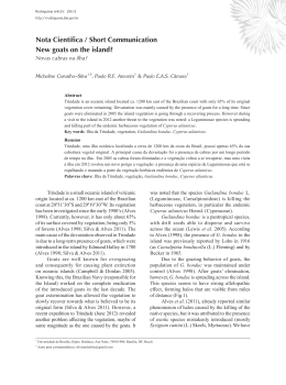
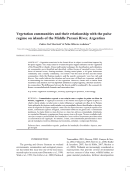
Predictability of Vegetation Cycles at Four Study Sites
in a Semi-Arid Region (Gourma, Mali)
Sylvain Mangiarotti1
Pierre Mazzega2,3
Cécile Dardel3
Eric Mougin3
Laurent Kergoat3
1
2
Centre d’Études Spatiales de la Biosphère, UPS-CNRS-CNES-IRD, Observatoire MidiPyrénées, 18 avenue Édouard Belin, 31401 Toulouse
Joint Mixt Laboratory OCE, UnB / IRD, LAGEQ, Instituto de Geociências - Universidade
de Brasília, Campus Darcy Ribeiro, Brasília - DF, Brasil
[email protected]
3
GET UMR5563, IRD-UPS-CNRS-CNES, OMP, 14 av. E. Belin 31400 Toulouse France
[email protected]
[email protected]
[email protected]
Abstract. We briefly present a nonlinear method for the prediction of vegetation states from Normalized
Difference Vegetation Index data, and its performance at four study sites in a semi-arid region (Gourma, Mali).
Based on 25 years of NDVI used in this study, this approach leads to a mean prediction error of approximately
20% (resp. 40%) RMS over a horizon of two weeks (resp. 4 weeks) and a spatial resolution of 24x24 km2. By
construction, the acquisition of new NDVI observations will improve these performances by allowing a finer and
more complete reconstruction (including rare events) of the multi-dimensional probability density function of the
vegetation states.
Keywords: vegetation cycle; semi-arid region; horizon of predictability; spatial scale; NDVI satellite data;
nonlinear prediction.
1. Introduction
In semi-arid regions, particularly in the Sahel, the intensity and distribution of precipitation
(Frappart et al., 2009) determines the primary production of vegetation. Livestock uses natural
pastures. Productivity of rainfed agriculture also depends strongly on the spatial and temporal
distribution of precipitations (Herrmann et al., 2005). The forecast of rain, but in fact more
directly the forecast of primary production with a sufficient anticipation (Maselli et al., 1992;
Balaghi et al., 2008) could condition strategies of transhumance routes or the choice of crop
or crop rotation of the populations involved in these survival or productive activities.
Two approaches attempt to produce assessment or forecasting of the vegetation cycles: a) the
models, relying on data (including observations from space: satellite imagery and radar
systems) and on sub-models of vegetation dynamics and radiative transfer, that propose a
representation of the processes involved and of their interactions so as to produce all the
vegetation state variables (biomass, leaf area index, etc.; e. g. Jarlan et al., 2003, 2008); b) the
approaches, like in this study, based on past chronic of data (here the vegetation index NDVI)
and on the observed 15-day to inter-annual variations of the signal, that attempt to infer the
future state of the vegetation over a more or less distant time-horizon.
However, both approaches face the intrinsic limits of predictability of the vegetation cycle
that some analysis, combining the deterministic (dynamical system; e. g. Abarbanel, 1996)
and stochastic (multivariate probability densities and fractal geometry, e. g. Diks, 1999)
paradigms, allows to quantify in the form of horizons of predictability. Then remains,
according to the prediction algorithm used, to determine the effective predictability (the upper
bound being set by the intrinsic predictability) of the vegetation cycle.
After a brief description of the data and data pre-processing in section 2, the theoretical
background of the forecasting approach is described in section 3, as is a description of the
methodology used to estimate the horizon of effective predictability, HE. The results are
presented and discussed in section 4 followed by a conclusion in section 5.
2. Normalized Difference Vegetation Index Data
Based on the radiometric data from the AVHRR (Advanced Very High Resolution
Radiometer) sensor onboard NOAA (National Oceanic Atmospheric Administration)
satellites 7, 9, 11, 14, 16 and 17, the NDVI product is produced by the Global Inventory
Modelling and Mapping Study (GIMMS) of the Global Land Cover Facility (GLCF,
www.landcover.org) (Tucker et al., 2004; 2005; Pinzon et al. 2005). The data used here cover
the period spanning from 1982 to 2006. Its spatial resolution is of 8×8 km2 which results from
the subsampling of initial 1.2 km² pixel data (Justice et al., 1989; James & Kalluri, 1994). To
reduce atmospheric interference and observation angle effects on the signal, the data are 15day composites selecting the maximum NDVI value for each pixel over fifteen days (Holben,
1986). Corrections account for sensor degradation over time as well as for the geometric
effects of the view and atmospheric aerosols resulting from eruptions. The area of study is
shown on Figure 1.
Figure 1: Location of the four
stations (1, 12, 17, 25) in the study
area centred on the Agoufou site of
the AMMA program (15.3°N,
1.5°W; see Mougin et al., 2009) in
the Gourma region. Before
analysing the time series, a preprocessing has been applied to the
data. A precise geo-referencing of
the image was carefully performed
based on clearly identifiable
reference points. The signal of the
four studied sites was then
aggregated by averaging the 9
closer pixels around the centred
one including the studied site,
leading to a new 24×24 km2
aggregated pixel.
A smoothing was also applied in order to reduce the additive noise. An estimate of this noise
level is provided in Table 1. The resulting data have been resampled with a sampling period
of 0.25 month. As will be seen later, the horizon of effective predictability (see Sec. 4) is
similar to the values in the range [0.23-0.67] months obtained at similar scales, say 16×16
km2 and 32×32 km2, by Mangiarotti et al. (2010; 2012).
Table 1: Sites numbers and coordinates, basic statistics of the aggregated time series (min,
max, mean and standard deviation), time delay τ obtained using the first minimum of the AMI
function, additive noise (in % of the original variance of the signal) removed by aggregating
and filtering the analysed signal and horizon of effective predictability.
Site
Latitude
Longitude
min max mean std Time
%
HE
#
(°N)
(°W)
delay τ
noise (month)
(month)
1
16.76
1.89
0.12 0.45 0.25 0.05 4.25
7.3
0.26
12
15.97
1.28
0.12 0.67 0.31 0.08 3.75
3.1
0.29
17
15.34
1.48
0.14 0.68 0.32 0.09 3.75
7.1
0.27
25
15.00
1.54
0.09 0.89 0.36 0.13 4.25
2.0
0.31
3. Nonlinear Data Analysis
NDVI time series of the four study sites are reproduced in Figure 2. We see in particular an
increase in the variance of the signal – dominated by an annual cycle – along the North (site
1) - South (site 25) gradient. The low primary productivity related to droughts is especially
marked during the period 1985-1988 in the Gourma (Heumann et al., 2007). In contrast some
years such as 1994 or 1999 exhibit a relatively high primary production.
Figure 2: Time series of normalized difference vegetation index measured from satellite for
sites 1 (top panel), 12 (second panel), 17 (third panel) and 25 (bottom panel).
However, our purpose here is not to conduct such analysis, but to provide a tool for
forecasting NDVI values which main steps of data processing are briefly described below.
Note that we here do not discuss the algorithms used in the data processing but we refer to the
a few useful references.
3.1 Reconstruction
The dependent variables describing the state of a dynamical system evolve on an attractor that
occupies a small part of the volume of phase space. Takens theorem (1981) shows that from
the knowledge of one of the variables x(t), it is possible to reconstruct in a pseudo phase space
an attractor diffeomorphic to the original attractor (that involves all the system state
variables). The existence of this diffeomorphism ensures that various geometric and statistical
properties (invariants) of the system dynamics can be inferred or quantified through the
analysis of this single data time series.
Figure 3: 3D reconstruction of the vegetation cycle attractors from NDVI
data time series at the study sites 1, 12, 17 and 25 (see Fig. 1).
For that purpose we built from the time series x(t) the vector of lagged variables
x(t ), x(t   ),..., x(t  ( DE  1) ) which each component is one coordinate of a point in the
pseudo-space of embedding dimension DE . The time delay  can be estimated from the
autocorrelation function of the time series, but in the presence of strong nonlinearities using
the first minimum of the average mutual information function is preferable (Fraser and
Swinney, 1986). Various algorithms also allow determining the embedding dimension DE (e.
g. Kennel and Abarbanel, 2002; Letellier et al., 2008). Figure 3 shows the portraits of the
vegetation cycle reconstructed at each study site from the time series of NDVI with an
embedding dimension DE  3 , the used time delays being given in Table 1.
3.2 Forecasting
The attractor is the fractal support of the probability density function (PDF) of the states of
the observed system. The approach used for the prediction is the following: we choose a date
t j from which we want to predict the state of the system at time t j  h .
To time t j corresponds a point on the reconstructed attractor. We then perform a selection of
k  1..K neighboring points
x(tk ), x(tk   ),..., x(tk  ( DE  1) )
on the reconstructed
trajectory. Prediction of the state at tk  h is made by weighting the K states of the
neighboring
points
propagated
along
the
attractor,
says
the
points x(tk  h), x(tk  h   ),..., x(tk  h  ( DE  1) ) . Figure 4 gives a geometric
representation of this method. Locally, the directions along which the observed segments of
trajectories are converging (resp. diverging) are tangent to the stable (resp. unstable)
manifolds on which the predictability of system states increases (resp. decreases).
Figure 4: Forecasting
approach based on an
empirical algorithm that
identifies
analogous
vegetation states already
visited in the embedding
space and use their
corresponding trajectory to
predict statistically the
future of the trajectory.
3.3 Effective Predictability
In the reconstruction process, the probability density function (PDF) of an additive noise data
is convolved with the PDF of the "signal" associated with the evolution of the system state
variables. Thus an observation error can induce a perturbation of the system along a direction
tangent to a stable (resp. unstable) manifold of the attractor, increasing (resp. decreasing) the
performance of the prediction with respect to its intrinsic predictability. Using only empirical
data, it is this effective predictability (taking into account the data errors, filtering applied to
reduce them, the characteristics of the signal sampling, etc.; Yu et al., 2000) that we estimate
here. Statistics for the predictive skill are based on the forecasting error e j h  , which is the
forecasting error at time t j  h when forecasting from time t j , with h being the horizon of
prediction. The forecasting error is defined as:
e j h  xˆ j h  x j h
(1)
where x j  h represents the data at time t j  h , and xˆ j h  is the forecast from t j to t j  h . The
% of error averaged along the attractor ph  is defined as follows:
(2)
ph   100   e2 (h) /  x2
where  x is the standard deviation of the original data time series, and  e h  is defined as

 e h   N 1  j e 2j (h)
N

1/ 2
(3)
where N is the number of data. Note that in practice, the systematic error
N
e h   N 1  j e j h  is very low ( e h  103 ).
N
j
4. Forecasting Error and Predictability of the Vegetation Cycle
The forecasting error and predictability of the observed vegetation cycle are dependent on the
scale of resolution of the NDVI data, on the embedding dimension, and on the chosen horizon
for prediction as we shall see here below.
4.1 Scale dependence of the forecasting error
We have shown elsewhere (Mangiarotti et al., 2010, 2012) that the predictability of a time
series of NDVI is related to the spatial resolution of the data. Indeed when the data are
aggregated over a large spatial area, the observed cycle looks like a periodic signal which is
associated with high predictability (at the expense of spatial resolution). On the contrary, the
use of non-averaged data time series leads to a lower predictability of the vegetation cycle but
with a higher spatial resolution of 8x8 km2. The intermediate scale – we use here – offers the
good compromise between good predictability and good spatial resolution of the NDVI.
The analysis of the forecasting error as a function of time (period 1982-2006) and of the
prediction horizon h exhibits strong intra-annual heterogeneity with in average a low
predictability (larger error) during rainy seasons and a high predictability (lower errors due to
less vegetation) in the dry season. Large inter-annual variability of the forecasting error is also
observed with positive errors corresponding to low rainfall years and negative errors
corresponding to high rainfall years. These results highlight the limits of the prediction
method that relies on past data (and observed events) but also its capacity to mechanically
improve with the addition of new data.
4.2 Model dimension and forecast accuracy
The embedding dimension DE of a white noise is infinite. Therefore the additional noise in
the data tends to increase the value of DE beyond the need for reconstruction of the attractor
of the (noise free) vegetation cycle. Figure 5 shows that the longer is the prediction horizon
(higher values of h), the higher is the embedding dimension that minimizes the prediction
error.
Figure 5: Optimal embedding dimensions as a function of horizon of prediction h (in month):
dimensions for which the minimum error is obtained (+/- 1%).
However a dimension DE between 4 and 6 covers a wide range of prediction horizon with an
acceptable error along the North-South gradient sites of Gourma.
4.3 Horizon of effective predictability
We here define the horizon of predictability HE as the horizon for which the forecasting error
doubles, assuming an exponential error growth rate. In practice, this parameter is computed
from the ratio of the increasing error between decades 1 and 2 (as the level of noise
corresponding to h = 0 is unknown) as follows:
1
(4)
H E  log( 2)log( p(2) / p(1)
where the % of error p(h) is defined in eq. 2. Figure 6 shows the prediction error (in RMS and
in %) as a function of the prediction horizon for each site. When going from the quasi-arid
North to the semi-arid South, the RMS error increases and the error relative to the variance of
the signal decreases. The values of HE for each site are between 0.26 and 0.31 months (see
Tab. 1). Now, if we think in terms of error in NDVI unit, the prediction can be useful for a
longer time horizon. For example if the acceptable level of error is 0.05 NDVI unit, the
horizon is in average about 2 months in the North of Gourma to 2 weeks in the South.
Figure 6: The forecasting RMS error (left panel) and the % relative forecasting error (right
panel), both corresponding to the optimal embedding dimension with a level of confidence of
75%, as a function of the horizon of prediction h (100= 1 month) for sites 1 (dashed magenta
line), 12 (light green line), 17 (dotted black line) and 25 (dark red line).
5. Conclusion
In average the prediction method presented here can anticipate by two weeks the vegetation
conditions with an RMS error of ~20% and a spatial resolution of 24x24 km2. This error
exhibits intra-annual and inter-annual oscillations, the exceptionally dry or wet years being
less well anticipated because of the rarity of their occurrence, particularly with regard to the
short series of available NDVI. However, the performance of the prediction method increases
with the acquisition of new data, diversifying the observed states of the system and increasing
the density of the empirically reconstructed attractor of the vegetation cycle. In addition, the
predicted values of NDVI can be used in a data assimilation scheme in a model of vegetation
dynamics to produce in advance the likely values of other state variables of vegetation (like
biomass, leaf area index, etc.).
Acknowledgments: This work was performed within the framework of the AMMA and ANR ECLIS projects.
Based on a French initiative, AMMA has been constructed by an international group and is currently funded by
large number of agencies, especially from France, the UK, the US and Africa. It has been the beneficiary of a
major financial contribution from the European Communities Sixth Framework Research Program. Detailed
information on scientific coordination and funding is available on the AMMA international web site
(https://www.amma-eu.org/).
6. References
Abarbanel, H.D.I. Analysis of Observed Chaotic Data. ISBN-0387983724, Springer, Berlin,
272 pp., 1996.
Balaghi, R.; Tychon, B.; Eerens, H.; Jlibene, M. Empirical regression models using NDVI,
rainfall and temperature data for the early prediction of wheat grain yields in Morocco. Int.
J. of Appl. Earth Obs. and Geoinformation, doi:10.1016/j.jag.2006.12.001, 2007.
Diks, C. Nonlinear time series analysis, World Scientific, Singapore, 209 pp., 1999.
Frappart, F. ; Hiernaux, P. ; Guichard, F. ; Mougin, E. ; Kergoat, L. ; Arjounin, M. ; Lavenu,
F. ; Koité, M. ; Paturel, J.E. ; Lebel, T. Rainfall regime over the Sahelian climate gradient
in the Gourma, Mali. Journal of Hydrology, 375 (1-2), p. 128–142, 2009.
Fraser, A.M.; Swinney, H.L. Independent coordinates for strange attractors from mutual
information, Physical Review A, 33, p. 1134–1140, 1986.
Herrmann, S.M.; Anyamba, A.; Tucker, C.J.. Recent trends in vegetation dynamics in the
African Sahel and their relationship to climate. Global Environmental Change, 15, p.
394–404, 2005.
Heumann, B.W.; Seaquist, J.W.; Eklundh, L.; Jönsson, P. AVHRR derived phenological
change in the Sahel and Soudan, Africa, 1982–2005, Remote Sens. Environment, 108 (4),
p. 385–392, 2007.
Holben, B.N. Characteristics of maximum-value composite images for temporal AVHRR
data. Int. J. Remote Sensing, 7, p. 1435–1445, 1986.
James, M.E.; Kalluri S.N.V. The pathfinder AVHRR land data set: an improved coarse
resolution data set for terrestrial monitoring. Int. J. Remote Sensing, 15 (17), p. 3347–
3363, 1994.
Jarlan, L. ; Mangiarotti, S. ; Mougin, E. ; Mazzega, P. ; Hiernaux, P. ; Le Dantec, V.
Assimilation of SPOT/VEGETATION NDVI data into a Sahelian vegetation growth model,
Remote Sens. Environment, 112, p. 1381–1394, doi: 10.1016/j.rse.2007.02.041, 2008.
Jarlan, L.; Mazzega, P.; Mougin, E.; Lavenu, F.; Marty, G.; Frison, P.L.; Hiernaux, P.
Mapping of sahelian vegetation parameters from ERS scatterometer data with an evolution
algorithm, Remote Sens. Environment, vol. 87, p., 72-84, 2003.
Justice, C.O.; Markham, B.L.; Townshend, J.R.G.; Kennard, R.L. Spatial degradation of
satellite data. Int. J. Remote Sensing, 10 (9), p. 1535–1561, 1989.
Kennel, M.B.; Abarbanel, H.D.I. False neighbors and false strands: A reliable minimum
embedding dimension
algorithm.
Physical
Review
E, 66,
p.
1–18,
doi:10.1103/PhysRevE.66.026209, 2002.
Letellier, C.; Moroz, I.M.; Gilmore, R. Comparison of tests for embeddings. Physical Review
E, 78, 026203, doi:10.1103/PhysRevE.78.026203, 2008.
Mangiarotti, S.; Mazzega, P. ; Jarlan, L. ; Mougin, E. ; Baup, F. ; Demarty, J. Evolutionary
Bi-Objective Optimization of a semi-arid vegetation dynamics model with NDVI and σ0
Satellite
data.
Remote
Sens.
Environment,
112,
p.
1365–1380,
doi:10.1016/j.rse.2007.03.030, 2008.
Mangiarotti, S. ; Mazzega, P.; Hiernaux, P. ; Mougin, E. The Vegetation Cycle in West Africa
from AVHRR-NDVI data: Horizons of predictability versus Spatial Scales. Remote Sens.
Environment, doi:10.1016/j.rse.2010.04.010, 2010.
Maselli, F.; Conese, C. ; Petkov, L. ; Gilabert, M.-A. Use of NOAA-AVHRR NDVI data for
environmental monitoring and crop forecasting in the Sahel. Preliminary results, Int. J.
Remote Sensing, 13(14), 2743–2749, doi: 10.1080/01431169208904076, 1992.
Mougin, E.; and 35 co-authors. The AMMA Gourma observatory site in Mali: relating
climatic variations to changes in vegetation surface, hydrology, fluxes and natural
resources. Journal of Hydrology, 375, 14–33, doi:10.1016/j.jhydrol.2009.06.045, 2009.
Pinzon, J.; Brown, M.E.; Tucker, C.J. Satellite time series correction of orbital drift artifacts
using empirical mode decomposition. In: N. Huang (Ed.), Hilbert-Huang Transform:
Introduction and Applications, p. 167-186, 2005.
Takens, F. Detecting strange attractor in turbulence, in Lecture Notes in Mathematics, 898,
Rand D. and L.S. Young eds., Springer Verlag, Berlin, p. 366–381, 1981.
Tucker, C.J.; Pinzon, J.E.; Brown, M.E. Global Inventory Modeling and Mapping Studies,
NA94apr15b.n11-VIg, 2.0, Global Land Cover Facility, University of Maryland, College
Park, Maryland, 04/15/1994, 2004.
Tucker, C.J.; Pinzon, J.E.; Brown, M.E.; Slayback, D.A.; Pak, E.W.; Mahoney, R.; Vermote,
E.F.; Saleous, N.E. An extended AVHRR 8-km NDVI dataset compatible with MODIS
and SPOT vegetation NDVI data. Int. J. Remote Sensing, 26:20, 4485–4498,
doi:10.1080/01431160500168686, 2005.
Yu, D.; Small, M.; Harrison, R.G.; Diks, C. An efficient implementation of the Gaussian
kernel algorithm in estimating invariants and noise level from noisy time series data,
Physical Review E, 61(4), 3750–3756, 2000.