434 Brazilian Journal of Physics, vol. 36, no. 2A, June, 2006 Effects of Varying Curvature and Width on the Electronic States of GaAs Quantum Rings A. Bruno-Alfonso and T. A. de Oliveira Departamento de Matemática, Faculdade de Ciências, UNESP - Universidade Estadual Paulista, 17033-360, Bauru, SP, Brazil Received on 4 April, 2005 Stationary states of an electron in thin GaAs elliptical quantum rings are calculated within the effective-mass approximation. The width of the ring varies smoothly along the centerline, which is an ellipse. The solutions of the Schrödinger equation with Dirichlet boundary conditions are approximated by a product of longitudinal and transversal wave functions. The ground-state probability density shows peaks: (i) where the curvature is larger in a constant-with ring, and (ii) in thicker parts of a circular ring. For rings of typical dimensions, it is shown that the effects of a varying width may be stronger than those of the varying curvature. Also, a width profile which compensates the main localization effects of the varying curvature is obtained. Keywords: Electronic states; GaAs elliptical quantum rings; Effective-mass approximation I. INTRODUCTION The stationary states of electrons confined in twodimensional rings have been studied for some special cases. Magarill et al. [1] and Berman et al. [2] have investigated elliptic rings of constant and varying width in the presence of a threading magnetic field. However, their theory is specific for the elliptical shape. Other groups [3, 4] have dealt with rings of arbitrary shapes and constant width. Circular rings with varying width in the presence of electric and magnetic fields have also been studied [5, 6]. In this work, it is presented a simple approach to the electron states in thin rings with arbitrary (but smooth) variations of curvature and width. The numerical results are given and discussed for elliptical rings. II. THEORY AND RESULTS Electronic states in GaAs are described within the effectivemass approximation. The attention is focused in a free motion on a ring-shaped planar strip. The motion in the third dimension is assumed to be separated. Hence, the two-dimensional stationary states satisfy µ 2 ¶ ~2 ∂ ∂2 − ∗ + ψ(x, y) = E ψ(x, y) , (1) 2m ∂x2 ∂y2 where m∗ is the electron effective mass in GaAs. Since the particle is confined in the ring, ψ(x, y) obeys Dirichlet boundary conditions. In the present work, the elliptical ring is the twodimensional region swept by a line segment whose midpoint describes an ellipse. This curve is the centerline of the ring and may be given by the parametric equations. x = a cos(θ), y = b sin(θ), 0 ≤ θ ≤ 2π , (2) where a and b are the semi-axes. The line segment is always perpendicular to the centerline and its length depends smoothly on θ. The curvature of the ellipse is given by £ ¤−3/2 k = ab a2 sin2 (θ) + b2 cos2 (θ) . (3) To obtain the wave function ψ(x, y), the curvilinear coordinates s and u are introduced. The coordinate s is the arc length measured counterclockwise along the ellipse from the point (x, y) = (a, 0). It is calculated as s= Z θ£ ¤1/2 a2 sin2 (t) + b2 cos2 (t) dt , (4) 0 and the perimeter L of the centerline is the value of s for θ = 2π. Then, the ring width w and the curvature k may be thought as functions of s. The coordinate u is the oriented distance of the point (x, y) to the centerline. The distance is measured in units of the width w corresponding to the value of s at the nearest point of the ellipse. It is positive (negative) for points outside (inside) the centerline. The Jacobian determinant of the (u, s) → (x, y) mapping is given by J = w (1 + uα), where α = wk. It should be positive for −1/2 ≤ u ≤ 1/2 and 0 ≤ s ≤ L. Otherwise, the inner boundary of the ring would not be well defined [4]. Hence, α ≤ 2 should apply for 0 ≤ s ≤ L. This condition imposes and upper bound for the ring width at each point of the centerline. In the new variables (u, s), the problem is simplified because the domain is a rectangular strip. However, the differential equation (1) has to be transformed accordingly. To calculate ψ(x, y) one may: (i) write the Laplace operator in the Beltrami form [3] for the curvilinear coordinates (u, s), (ii) √ substitute ψ(x, y) = f (u, s)/ J, (iii) perform √ the approximation f (u, s) = hn (u)g(s), where hn (u) = 2 sin(nπ(u + 1/2)) behaves as the nth transversal mode, (iv) apply the variational method to derive an equation for the longitudinal wave function g(s), and (v) solve the resulting ordinary differential equation with the boundary conditions g(L) = g(0) and g0 (L) = g0 (0). The longitudinal equation is " # 6 d d ~2 − In (α) + ∑ vq g(s) = E g(s) , (5) 2m∗ ds ds q=1 where E =E− ~2 n2 π2 , 2m∗ w̄2 (6) A. Bruno-Alfonso and T. A. de Oliveira 435 with w̄ being mean width of the ring, and Z 1/2 −1/2 h2n (u)(1 + αu)−2 du . (7) Note in Eq. (6) that E may be interpreted as the longitudinal energy, with ~2 n2 π2 /(2m∗ w̄2 ) being the energy of the nth transversal mode. Also, In (α) in the first term of Eq. (5) leads to an arc-length-dependent longitudinal mass. The longitudinal potential is the sum of six terms, where k2 In (α) , 4 (8) wk̈ 0 5w2 k̇2 00 In (α) − I (α) , 4 24 n (9) v1 = − v2 = − µ v3 = n π 2 2 v4 = − 1 1 − w2 w̄2 160 HaL ¶ , ¤ ẅk 0 ẇk̇ £ 0 I (α) + αIn00 (α) − I (α) , 2 n 2 n (10) (11) 80 yHnmL In (α) = width oscillates with a very small amplitude. As such variations are not apparent in Fig. 2(a), the width profile is depicted in Fig. 2(c). The probability distribution of the ground state in the elliptical ring with a = 150 nm, b = 50 nm, w̄ = 15 nm, and sinusoidal width oscillations of amplitude 0.1 nm is displayed in Fig. 2(b). Interestingly, it does not show larger values where the curvature is larger. Indeed, the probability is higher where the ring is wider, resembling Fig. 2(a). In these cases, v3 is the dominant term in the longitudinal potential. As width variations larger than 0.1 nm are often present in grown or fabricated ring and wave guides, the experimental detection of electron confinements due to curvature variations may be difficult. 0 -80 £ ¤ v5 = 3In (α) + 2αIn0 (α) , 2 4w ẇ2 (12) -160 and -160 w2 Z 1/2 −1/2 u2 h2n (u)(1 + αu)−2 du . (13) Here, the dots over w and k represent derivatives with respect to the arc-length s. The numerical results presented below correspond to the ground state of the particle. Hence, the fundamental mode n = 1 is taken for the transversal motion. The electron effective mass in GaAs is taken as m∗ = 0.067m0 , where m0 is the electron mass. The probability distribution of the ground state in a circular ring of radius a = b = 106.4 nm and constant width w = 15 nm is represented in Fig 1(a). Due to the rotational symmetry of the ring, the probability is independent of the electron position along the ring. In contrast, the probability density of the ground state in an elliptical ring of constant width should have its larger values in the regions of larger curvature [1, 4]. This is clearly shown in Fig. 1(b) for a = 150 nm, b = 50 nm and w = 15 nm. In both of these cases, the perimeter of the centerline is L = 668.2 nm and v1 is the dominant term in the longitudinal potential. The variations in the width of the ring may produce strong effects on the wave functions [1]. To illustrate this, the ring centerlines and the mean width w̄ = 15 nm in Fig. 1 are considered. However, the width profile is taken as w = [15 − 0.1 cos(4πs/L)] nm. The ground-state probability distribution in the circular ring is displayed in Fig. 2(a). There, the probability is higher in the thicker parts of ring. Note that the -80 0 xHnmL 80 60 yHnmL v6 = n2 π2 ẇ2 160 HbL 30 0 -30 -60 -160 -80 0 xHnmL 80 160 FIG. 1. The probability density of the ground state in (a) a circular ring with radius a = b = 106.4 nm and (b) an elliptic ring with semiaxes a = 150 nm and b = 50 nm. Both rings have equal perimeters L = 668.2 nm and a constant width w = 15 nm. Darker tones represent larger relative values. At this point, one may wonder if for a given mean width w̄ there exists a width profile which compensates the main localization effects of the varying curvature. To obtain such a profile, one may retain the terms v1 and v3 in the effective longitudinal and assume that v1 + v3 does not depend on s, namely, µ ¶ k2 1 1 βn2 π2 − In (α) + n2 π2 − = , (14) 2 2 4 w w̄ w̄2 where β is a constant. Moreover, α is assumed to be sufficiently small, so that In (α) ≈ 1 in the kinetic term of Eq. (5) and in the first term of Eq. (14). Then, ¶−1/2 µ w̄2 k2 w = w̄ 1 + β + 2 2 , (15) 4n π 436 Brazilian Journal of Physics, vol. 36, no. 2A, June, 2006 w̄ = Z 1 L L w ds . (16) 0 yHnmL and β is determined from 160 HaL 60 30 0 -30 -60 -160 HaL -80 0 xHnmL 80 160 15.1 HbL wHnmL yHnmL 80 0 15.0 14.9 -80 14.8 0.0 0.25 0.50 sL 0.75 1.0 -160 -160 -80 0 xHnmL 80 yHnmL 60 160 HbL 30 0 -30 -60 -160 -80 0 xHnmL 80 160 15.1 HcL wHnmL FIG. 3. (a) The probability density of the ground state in an elliptic ring with semi-axes a = 150 nm and b = 50 nm, and mean width w̄ = 15 nm. Darker tones represent larger relative values. (b) The width as a function of the arc-length s along the centerline. This profile has been chosen to compensate the main effects of the varying curvature. 15.0 14.9 14.8 0.0 0.25 0.50 sL 0.75 1.0 FIG. 2. The probability density of the ground state in (a) a circular ring with radius a = b = 106.4 nm and (b) an elliptic ring with semiaxes a = 150 nm and b = 50 nm. Both rings have equal perimeters L = 668.2 nm and mean width w̄ = 15 nm. Darker tones represent larger relative values. (c) The width dependence on the arc-length s along the centerline, given by w = [15 − 0.1 cos(4πs/L)] nm. The Fig. 3(a) shows the probability density for the ground state in a ring with the same centerline as those considered in Figs. 1(b) and 2(b), and the same mean width w̄ = 15 nm. There, the probability is essentially independent of the position along the ring, resembling Fig. 1(a). The width profile is depicted in Fig. 3(b) and has been calculated by Eq. (15), with β ≈ −0.0015 [see Eq. (16)]. Note that, according to Eq. (15), when the compensation occurs the ring is thinner where the centerline curvature is larger. For future numerical comparisons, Table I contains the longitudinal energy of the electron states shown in the figures above. The transversal energy in all cases is 24.9439 meV. Table I. The longitudinal energy of the electron states shown in Figures 1, 2 and 3. Panel 1(a) 1(b) 2(a) 2(b) 3(a) E (meV) -0.0126 -0.0600 -0.1747 -0.1643 -0.0383 III. CONCLUSIONS A simple equation has been derived to calculate stationary states of an electron in a thin GaAs ring, where both the curvature and the width may vary arbitrarily (but smoothly). Numerical results were presented for elliptical rings of varying width. The ground-state probability density was shown to be larger where the curvature is larger in a constant-width ring, and in thicker parts of a circular ring. More interestingly, the results for elliptic rings with varying width show that (i) the effects of very small variations of the width can be more important than those of the curvature changes, and (ii) one may obtain the width profile which compensates the main localization effects of the curvature variations. Namely, A. Bruno-Alfonso and T. A. de Oliveira 437 the ring should be appropriately thinner where the curvature of the centerline is larger. A simple expression for such a profile has been given. These later results have implications for nanostructure device engineering. Acknowledgments [1] L. I. Magarill, D. A. Romanov, and A. V. Chaplik, JETP 83, 361 (1996). [2] D. Berman, O. Entin-Wohlman, and M. Ya. Azbel, Phys. Rev. B 42, 9299 (1990). [3] I. J. Clark and A. J. Bracken, J. Phys. A: Math. Gen. 29, 339 (1996). [4] D. Gridin, A. T. I. Adamou, and R. V. Craster, Phys. Rev. B 69, 155317 (2004). [5] L. A. Lavenère-Wanderley, A. Bruno-Alfonso, and A. Latgé, J. Phys.: Condens. Matter 14, 259 (2002). [6] A. Bruno-Alfonso and A. Latgé, Phys. Rev. B 71, 125312 (2005). The authors are grateful to the Brazilian Agency FAPESP and the PIBIC/UNESP Program for financial support.
Download