MEAN AND RICCI CURVATURE OF SURFACES
THOMAS SWIFT
Abstract. In this paper, we take an in-depth look of various curvature measures for curves and surfaces. We start by defining what curvature is and
how to calculate it for space curves. After reviewing generalized curvature for
curves embedded in spaces of arbitrary dimension, we use the rest of the paper to discuss different curvature measures computed on surfaces, which is the
focus of the paper. In examining surfaces, we first define the first and second
fundamental forms of a surface as they are intimately related to every concept
of curvature defined for surfaces. Using these forms, we describe the normal
curvature of a surface, and briefly mention the geodesic curvature as well. We
then define the principal curvatures both geometrically in terms of the normal
curvature, and algebraically through the shape operator, or Weingarten Map.
Our definitions for the Gaussian and mean curvatures of a surface then directly
come from these principal curvatures. By looking at surfaces which have zero
mean curvature, we quickly overview minimal surfaces. We then conclude the
paper by defining the Ricci curvature tensor for a surface, which is defined in
terms of the Riemann curvature tensor, which is in turn defined in terms of the
Christoffel symbols, which come directly from the surface’s first fundamental
form.
1. Introduction
Curvature is a mathematical concept which has been around for thousands of
years. Curvature is used to relate the amount of bending of an object at each
point on the object, possibly with respect to a given direction depending on the
dimension of the object. The initial objects of study with respect to their curvature
were curves, the simplest such object, being only one-dimensional. The notion of
curvature is very important, as it completely determines a curve, up to rigid motion, as stated in the fundamental theorems of plane and space curves (here, rigid
motion indicates a distant-preserving transformation consisting of translations and
rotations). The origins of the study of curvature come from the Ancient Greeks,
who noticed the difference a line, which doesn’t bend at all, and a circle, which has
a constant amount of bending at each of its points. Aristotle expanded upon these
observations by classifying every curve as either straight, circular, or mixed, which
formed the basis for studying curvature. [10]
In the third century B.C., Apollonius of Perga advanced the study of curvature
by studying conic sections and discovering that there is exactly one normal line
at each point of a conic. He also determined procedures for finding the radius
of curvature of a curve, such as by using the method of exhaustion, which paved
the way for later discoveries made by Newton and Huygens, who used remarkably
similar methods to do this calculation. In the fourteenth century, Nicole Oresme,
through drawing graphs, noticed that if two curves are tangent to each other at a
point and one lies inside the other (that is, on the other curve’s concave side), the
1
2
THOMAS SWIFT
inner cuve bends more than the outer curve. This is very intutive and easy to see
graphically. Look at the bending of the parabolas y = x2 and y = 2x2 at the origin,
for example, which is shown in Figure 1.1 This observation led him to propose that
the curvature of a circle is simply the multiplicative inverse of its radius. Circa the
year 1600, Johannes Kepler introduced the notion which later became known as
the circle of curvature when he he constructed a circle tangent to a given point of
a curve, which he used to approximate the curve. [10]
Figure 1.1. Here, we see the difference in the amount of bending of the parabols
y = x2 and y = 2x2 at the origin. From pure observation, we notice that the inner
parabola y = 2x2 has the greater degree of bending of the two curves. This can
be verified algebraically, as it has curvature 4 at the origin, while y = x2 only has
curvature 2.
Figure 1.2. The circle of curvature, or osculating circle, at a point P on an
arbitrary curve C, first used by Kepler. The radius of this circle, known as the
radius of curvature of C at P , is labeled by r. These terms and ideas were formalized
by later mathematicians, such as Isaac Newton.
Significant advances in the field of curvature were made with the advent of analytic geometry. Renes Descartes and Pierre de Fermat, two of the first analytic
geometers, devised a way to express a generic curve algebraically. This, of course,
was a highly significant and necessary step, as this algebraic representation was later
needed in order to rigorously describe the curvature of a general curve through calculus. The progress of these mathematicians, however, was greatly hindered by the
lack of the mathematical constat π in their analysis. [10]
Calculus was then invented in the late seventeenth century. Calculus, being
founded on the concepts of limits and infinitesimals, was a natural way to descibe
MEAN AND RICCI CURVATURE
3
curvature. Since two general curves have different magnitudes of bending at each
of their points, it was necessary to look at an infinitemsimal piece of a curve surrounding one of its points in order to accurately describe the curve’s curvature at
that point. Calculus was the perfect tool to accomplish this. [10]
Isacc Newton, co-inventor of calculus, began his investigation of curvature by
considering the following elementary facts and observations: the curvature of a
circle is constant and is the multiplicative inverse of its radius, and the largest
circle whch is tangent to a curve at a point and lies on its concave side has the same
curvature as the curve at that point, where the center of this circle is called the
center of curvature. Using infinitesimals, Newton described the center of curvature
at a given point on a curve as the point of intersection of the normals of two
points an infinitesimal distance from the given point on either side of it. Using
this definition, Newton developed a formula for the radius of curvature of a curve
at a point. However, Newton’s curvature formula was problematic for points of
inflection. Using calculus, as well as his own observations, Newton saw that curves
behave like lines in the infinitesimally small regions near their inflection points, as
we see in Figure 1.3. However, lines have an infinite radius of curvature, giving these
points on the curve an infinite radius of curvature, and so making the curvature
undefined. Newton also noticed that he could apply his methods of finding extrema
of functions from calculus, by setting the function’s derivative equal to 0, to find
the points where the curve bended the most and the least. [10]
Figure 1.3. The graph of an arbitrary curve. We see that the curve behaves like a
straight line at its point of inflection. This graph also illustrates Newton’s method
of finding maxima and minima by setting the function’s derivative equal to 0, as
we see that the tangent lines at this function’s extrema are clearly both horizontal
(have zero slope).
In 1731, Alexis-Claude Clairaut became the first geometer to study the curvature
of space curves, curves embedded in a three-dimensional space. Clairaut studied
these curves by taking DesCartes’ method of taking these space curves and projecting them onto two perpendicular planes, where the projections could be treated
as simple plane curves. He noticed that space curves have two different curvature
measures at each of their points. The second of these, which is not applicable to
plane curves and is new to space curves, he called the torsion, which measures how
quickly the curve’s osculating plane changes, which is the plane formed by the unit
tangent and unit normal vectors at a given point. This realization that an object
could have different curvature measures influenced the work of later geometers,
4
THOMAS SWIFT
such as Gauss, who extended the study of curvature to two-dimensional objects,
surfaces. [10]
The next mathematician to make a significant contribution towards the study of
curvature was Leonhard Euler. It was Euler who came up with the theorem that
if a curve is given in terms of a parameterization, then the curvature equals the
magnitude of the second derivative of this parameterization. That is, if we have
C = r(t) for a curve C, then the curvature κ is given by κ(t) = |r00 (t)| for all t in
the curve’s domain (we note that this only holds for unit-speed parameterizations
of curves). This was a hugely important discovery since parameterized curves are
ubiquitous in modern differential geometry. He also created a new way to define a
curve’s curvature. At a given point p on a curve, Euler would take the unit tangent
vector at p and assign it a point on the unit circle, which would encode the direction
of that vector. This function is known as Euler’s map. The curvature was then the
infinitesimal change of the angle of the tangent vector divided by the infinitesimal
change of the arc length, or dθ
ds . [10]
In the late eighteenth and early nineteenth centuries, Karl Gauss caused drastic
advancements in differential geometry by studying the curvature of surfaces rather
than curves. Gauss made many important contributions to differential geometry.
Firstly, he invented the Gauss Map, which generalizes Euler’s Map from the one
dimensional unit circle to the two dimensional unit sphere. The Gauss Map maps
the unit normal vectors of a surface, rather than the unit tangent vectors of a curve.
Gauss also invented the Gaussian curvature for a point on a surface, which is the
product of that point’s principal curvatures, the maximum and minimum curvatures of all curves on the surface which go through the point. In Gauss’ Theorem
Egregium, he is able to write the Gaussian curvature solely in terms of the components of the first fundamental form matrix of the surface and its derivatives, which
means that it is an intrinsic measure of curvature which is invariant to the space
the surface is embedded in. [10]
Sophie German worked with a different kind of surface curvature in her research,
which was related to the Guassian curvature. Using the same principal curvatures
which Gauss took the product of to find the Guassian curvature, German instead
took the average of these maximum and minimum curvatures. This new quantity
is known as the mean curvature of a surface at a point [11]. The mean curvature is
important because it is used to find objects called minimal surfaces, which are surfaces which have zero mean curvature everywhere. These objects were historically
called minimal surfaces because they minimized the surface’s surface area given a
specific boundary or constraint. However, this is not always the case and having
mean curvature be everywhere zero is the sole condition for a surface to be minimal.
Examples of such surfaces will be given later in the paper. [1]
In 1854, Bernhard Riemann generalized Gauss’ work on surfaces to arbitrary
n-dimensional objects. In doing so, he defined the concept of a differentiable manifold equipped with an inner product, or Riemannian metric, which are now called
Riemannian manifolds. Most importantly, he, along with Elwin Christoffel, defined
the Riemann curvature tensor, or Riemann-Christoffel tensor, for a point on an
MEAN AND RICCI CURVATURE
5
n-dimensional manifold. Christoffel is the mathematician for which the Christoffel symbols are named, which are used in defining the Riemann curvature tensor.
This tensor is a collection of scalars which specifies the amount of bending of the
manifold at a given point. For manifolds of higher dimension than two, the Gauss
curvature of the manifold is known as the manifold’s sectional curvature. [13, 15]
Gregorio Ricci-Curbastro then introduced Ricci curvature. Ricci developed Ricci
curvature because he noticed that if M is a Riemannian manifold, then M doesn’t
have an inherent second fundamental form, and therefore doesn’t have have any
prinicpal curvatures or directions which come from the eigenvalues and eigenvectors of the matrix reprsenetation of this form, unlike when M is a hypersurface (a
surface of dimension n − 1 embedded in a space of dimension n). This was very
problematic. However, he noticed that he could contract the Riemann curvature
tensor (take its trace) to get a two-dimensional tensor which had these nice properties [13]. Ricci curvature has applications to general relativity, where it is a term
in the Einstein field equations, which relate the ricci tensor, the scalar curvature
(contraction of the ricci tensor), and the metric to the Einstein tensor and energymomentum (stress-energy) tensor. [8, 17]. It also is used in the Ricci flow equation
which was introduced by Richard Hamilton. [16]
Ricci flow is an analog of the heat equation, which states that heat moves through
an object until a state of equilibrium is reached in which the temperature, amount
of heat, is constant throughout the body. Similarly, in the case of two-dimensional
manifolds at least, Ricci flow deforms the Riemannian metric of the manifold into
a metric which has constant Ricci curvature. This is known as the uniformization
theorem. In the general case of n-dimensional Riemannian manifolds, Ricci flow is
a process which stretches the metric in the directions where the Ricci curvature is
negative, and contracts it in the directions where the Ricci curvature is positive.
This has the result of increasing and decreasing, respectively, the distance between
points on the manifold. The stretching and contracting of the metric is greater the
higher the magnitude of the Ricci curvature. [12, 16]
2. Curvature of Curves
3
Let C = r(t) : R → R be a space curve. Then, the curvature of C is defined as
the rate of change of the direction of C with respect to its arc length. That is, with
respect to the unit tangent vector T , which specifies direction, and the arc length
s, the curvature is defined as
dT ,
(1)
κ = ds which alternatively can be written as
κ=
|T 0 (t)|
|r0 (t)|
and
κ=
|r0 (t) × r00 (t)|
.
|r0 (t)|3
(2)
Rt
Here, the arc length function s(t) of r(t) is defined as s(t) = a |r0 (u)| du, where a is
the point from which we start measuring the arc length. Note that in most cases,
we let a = 0. [5, 14]
6
THOMAS SWIFT
The curvature is a key component of the Frenet-Serret formulas, which specify
the relationship between the components of the Frenet frame of a curve and their
derivatives. The Frenet frame of a curve C consists of the unit tangent vector T ,
the unit normal vector N , and the binormal vector B of C. These three vectors
together define an orthonormal basis for any point on C. Figure 2.1 below shows
the Frenet frame for a helix at several different points along its path.
The Frenet-Serret formulas can then be expressed in matrix notation as
0
T
0
vκ
0
T
N 0 = −vκ
0
vτ N ,
(3)
B0
0
−vτ 0
B
where v = |r0 (t)| is the speed of C and τ is the torsion of C. If C is parameterized
with respect to arc length, and thus v(t) = 1 ∀t, these formulas simplify to
0
T
0
κ 0
T
N 0 = −κ 0 τ N .
(4)
B
0 −τ 0
B0
[9, 14]
Figure 2.1. The Frenet Frame of T, N, and B vectors moving along a helix
Example 2.1. Consider the helix in Figure 2.1 which can be parameterized by
r(t) =< cos t, sin t, t >. We want to calculate the Frenet frame for this helix, as well
as its curvature and torsion.
We first reparameterize the helix with respect to its arc length to simplify
the cal√
culations. We see that r0 (t) =< − sin t, cos t, 1 > and so |r0 (t)| = 2. Thus, its
√
R t√
arc length is s(t) = 0 2 du = 2t. Thus, we have t = √s2 , and so we obtain
r(t(s)) = r(s) =< cos( √s2 ), sin( √s2 ), √s2 > It can be easily verified that |r0 (s)| = 1,
and so r(s) is indeed a unit speed curve.
We now calculate the T , N , and B vectors constituting the Frenet frame of the
helix. We see that
T (s) = r0 (s) =< − √12 sin( √s2 ), √12 cos( √s2 ), √12 >, and therefore
N (s) =
T 0 (s)
|T 0 (s)|
=
<− 12 cos( √s2 ),− 21 sin( √s2 ),0>
1
2
=< − cos( √s2 ), − sin( √s2 ), 0 >.
B(s) is then given by B(s) = T (s) × N (s) =< √12 sin( √s2 ), − √12 cos( √s2 ), √12 >.
Using the Frenet formulas (4), we calculate the curvature to be κ = κ(s) =
T 0 (s)N (s) =< − 12 cos( √s2 ), − 12 sin( √s2 ), 0 > · < − cos( √s2 ), − sin( √s2 ), 0 >= 12 ,
MEAN AND RICCI CURVATURE
7
and the torsion to be τ = τ (s) = −B 0 (s)N (s) = − < 21 cos( √s2 ), 12 sin( √s2 ), 0 > ·
< − cos( √s2 ), − sin( √s2 ), 0 >= 12 .
We can verify the value of the curvature through (2), which gives us,qin the case of
unit speed curves, κ = |T 0 (s)| = | < − 12 cos( √s2 ), − 12 sin( √s2 ), 0 > | =
1
4
= 12 .
We now look at generalized curvature for curves embedded in n-dimensional
space. Let C = r(s) be a curve in Rn which is parameterized by its arc length
s. The Frenet frame (e1 (s), e2 (s), . . . , en s(s)) is then constructed from the first n
derivatives of C,
(r0 (s), r00 (s), . . . , rn (s)), by the Gram-Schmidt process.
This process starts by defining the unit tangent vector as the first component of
the Frenet frame e1 (s), as it is for curves in R3 , which is given by e1 (s) = r0 (s).
Next, the unit normal vector corresponds to the second Frenet vector e2 (s), which
is defined as e2 (s) = r00 (s) − < r00 (s), e1 (s) > e1 (s), which is then divided by its
length to normalize the vector. This vector and the rest of the vectors in the Frenet
frame are defined by
ei (s) =
eˆi (s)
,
|eˆi (s)|
eˆi (s) = ri (s) −
i−1
X
< ri (s), ej (s) > ej (s),
(5)
j=1
where < ·, · > is the inner product defined on Rn , which is simply the dot product.
Additionally, the generalized curvature functions, or Frenet curvatures, κi (s) are
defined by
κi (s) =< e0i (s), ei+1 (s) >,
1 6 i 6 n.
(6)
[6, 9] If C is not parameterized with respect to arc length, then the generalized
curvature functions take the form
< e0i (t), ei+1 (t) >
κi (t) =
, 1 6 i 6 n − 1.
(7)
|r0 (t)|
Using the generalized curvature functions, a generalized version of the Frenet-Serret
formulas can be written as follows
0
κ1 (s) 0
···
0
..
0
..
..
−κ1 (s)
e1 (s)
.
.
e1 (s)
.
..
..
..
(8)
. = 0
. .
.
0
0
.
en (s)
en (s)
..
κn−1 (s)
0
···
0 −κn−1 (s)
0
[2, 9]
3. Curvature of Surfaces
We now turn our attention to describing the curvature of a surface. Let S =
f (u, v) = (x(u, v), y(u, v), z(u, v) be a regular surface embedded in R3 . In order to
describe the curvature of S, it is first necessary to discuss the fundamental forms
of S.
The first fundamental form of a suface S is defined as the restriction of < ·, · > to
all tangent planes of S, where < ·, · > is the Euclidean inner product in R3 . That
8
THOMAS SWIFT
is, the first fundamental form, denoted by I, is given by I(x, y) =< x, y > for any
two tangent vectors x, y ∈ Tp S for some p. It describes the intrinsic geometry of
a surface. Because S is regular, fu and fv are linearly independent, and so form
a basis for any tangent plane Tp S at a point p on S. Thus, the first fundamental
form can be expressed in this basis as the symmetric matrix
I(fu , fu ) I(fu , fv )
E F
I=
=
,
(9)
I(fv , fu ) I(fv , fv )
F G
where E = fu · fu , F = fu · fv = fv · fu , and G = fv · fv . We note that the matrix I
representing the first fundamental form is also referred to as the metric tensor gij
for 1 6 i, j 6 2, as it completely determines the metric of S. [14, 4, 3]
Example 3.1. Calculate the first fundamental form of the sphere of radius r Sr2
parameterized by f (θ, φ) =< r cos θ sin φ, r sin θ sin φ, r cos φ >, where 0 < θ <
2π, 0 < φ < 2π.
We first find the partial derivatives of Sr2 , which are given by
fθ =< −r sin θ sin φ, r cos θ sin φ, 0 > and
fφ =< r cos θ cos φ, r sin θ cos φ, −r sin φ > .
Then, E, F , and G are given by
E = fθ · fθ
=< −r sin θ sin φ, r cos θ sin φ, 0 > · < −r sin θ sin φ, r cos θ sin φ, 0 >= r2 sin2 φ,
F = fθ · fφ
=< −r sin θ sin φ, r cos θ sin φ, 0 > · < r cos θ cos φ, r sin θ cos φ, −r sin φ >= 0, and
G = fφ · fφ
=< r cos θ cos φ, r sin θ cos φ, −r sin φ > · < r cos θ cos φ, r sin θ cos φ, −r sin φ >= r2 .
Thus, the first fundamental form of Sr2 is given by
2 2
r sin φ 0
I=
0
r2
Now, it is also important to discuss the second fundamental form of S, which
describes the extrinsic geometry of a surface with respect to the space it is embedded
in. The second fundamental form of a surface S, denoted by II, is defined as
II(x, y) =< s(x), y > for any two tangent vectors x, y ∈ Tp S for some p. Here,
s is the shape operator, or Weingarten Map, defined in terms of the directional
derivative by s(x) = −∇x n, where n is the unit normal vector of S given by
v
n = |ffuu ×f
×fv | . We recall that to calculate the directional derivative of a vector field F
along a surface S at a point p in the direction of v ∈ Tp S, we calculate the derivative
of the restriction of F to a curve α(t) on S which passes through p and which has
its tangent vector at p in the direction of v. That is, ∇v F = (F ◦ α(t))0 (0), where
α : (−, ) → S is a curve on S such that α(0) = p and α0 (0) = v. We note that the
second fundamental form II has a natural connection with the first fundamental
form I since we can write II(x, y) = I(s(x), y). The second fundamental form can
MEAN AND RICCI CURVATURE
also be expressed in the {fu , fv } basis as the symmetric matrix
II(fu , fu ) II(fu , fv )
L M
II =
=
,
II(fv , fu ) II(fv , fv )
M N
9
(10)
where L = nu ·fu = fuu ·n, M = nu ·fv = fuv ·n = fvu ·n, and N = nv ·fv = fvv ·n.
We note that these simplifications of L, M , and N are possible because the shape
operator is self-adjoint, and so < s(x), y >=< x, s(y) > ∀x, y ∈ TpS . [4, 7, 14]
Example 3.2. Calculate the second fundamental form and shape operator (Weingarten Map) of the sphere of radius r Sr2 parameterized as above.
To find the second fundamental form of Sr2 , we calculate its second order partial
derivatives, which are
fθθ =< −r cos θ sin φ, −r sin θ sin φ, 0 >,
fθφ = fφθ =< −r sin θ cos φ, r cos θ cos φ, 0 >, and
fφφ =< −r cos θ sin φ, −r sin θ sin φ, −r cos φ > .
We also calculate its normal vector which is given by
n̂ = fθ ×fφ =< −r sin θ sin φ, r cos θ sin φ, 0 > × < r cos θ cos φ, r sin θ cos φ, −r sin φ >
=< −r2 cos θ sin2 φ, −r2 sin θ sin2 φ, −r2 sin φ cos φ >. We then normalize n̂ to get
the unit normal vector, n =< − cos θ sin φ, − sin θ sin φ, − cos φ >, and then negate
it to get the outward pointing unit normal n =< cos θ sin φ, sin θ sin φ, cos φ >. L,
M , and N are then given by
L = fθθ · n
=< −r cos θ sin φ, −r sin θ sin φ, 0 > · < cos θ sin φ, sin θ sin φ, cos φ >= −r sin2 φ,
M = fθφ · n
=< −r sin θ cos φ, r cos θ cos φ, 0 > · < cos θ sin φ, sin θ sin φ, cos φ >= 0, and
N = fφφ · n
=< −r cos θ sin φ, −r sin θ sin φ, −r cos φ > · < cos θ sin φ, sin θ sin φ, cos φ >= −r.
Thus, the second fundamental form of Sr2 is given by
−r sin2 φ 0
II =
0
−r
We see that the sphere has the special relationship that II(x, y) = − 1r I(x, y). That
is, its first and second fundamental forms are constant multiples of each other. This
will easily be explained when we determine the shape operator for the sphere.
We now note that for any point on the sphere p = f (θ, φ) for some θ, φ, n(p) =
1
1
r f (θ, φ) = r p. That is, each point on the sphere is its own normal vector (divided by the sphere’s radius to normalize its length). Using the definition of
the directional derivative as stated before, we then have, for x ∈ Tp Sr2 , s(x) =
−∇x n = −(N ◦ σ(t))0 (0) for σ : (−, ) → Sr2 such that σ(0) = p and σ 0 (0) = x.
However, since n(p) = 1r p ∀p ∈ Sr2 , we see that (n ◦ σ(t)) = σ(t)
r , and so
σ(t) 0
1 0
1
s(x) = −( r ) (0) = − r σ (0) = − r x. Thus, the shape operator explains the relationship between the first two fundamental forms of Sr2 , as II(x, y) =< s(x), y >=
< − 1r x, y >= − 1r < x, y >= − 1r I(x, y).
10
THOMAS SWIFT
Now that we have defined the fundamental forms of S, we can use them to
define various curvature measures for S. The first of these is the normal curvature
of a curve on S. Let α(t) = f (u(t), v(t)) be a curve on S with unit speed. We
can then define the Darboux frame, a moving frame which generalizes the Frenet
frame, as the orthonormal basis {α0 , n, n × α0 }, where n is the unit normal vector
of S as previously defined and α0 is the unit tangent vector, since α is unit speed.
Also, since α has unit speed, α00 is orthogonal to α0 . Thus, α00 can be written as
a linear of combination of n and n × α0 , the coefficients of which are defined to
be the normal curvature, κn and the geodesic curvature, κg , respectively. That is,
α00 = κn n + κg (n × α0 ). This relationship is illustrated in Figure 3.1. Because n and
n × α0 are orthogonal vectors, by separately multiplying both sides of the previous
equation by these vectors, we see that the normal curvature and geodesic curvature
can be written as
κn = α00 · n and κg = α00 · (n × α0 ).
(11)
0
00
We note that, since α has unit
speed,
we
have
T
(t)
=
α
(t),
and
thus
the
curvature
q
of α is simply κ = |α00 | = κ2n + κ2g . Hence, we see that the normal curvature is
the component of the curvature of α in the direction of n. We can also define the
normal curvature in terms of the second fundamental form of S by κn = Ldu2 +
2M dudv + N dv 2 , which can be expressed in matrix notation as
L M
du
κn = du dv
.
(12)
M N
dv
[7]
Figure 3.1. Normal and geodesic curvature of 2 different points on the same curve
on a surface, shown as components of the curve’s second derivative x00
Additionally, we use κn to define the normal curvature of S in the direction of a
unit tangent vector T = α0 at a given point p on S, which measures the curvature of
S in the direction of T . That is, for a point p on S, we take the normal plane of S at
p to be the plane spanned by the surface normal n(p) and the tangent vector T to S
at p. The intersection of this plane with S will then define a curve α on S oriented
in the direction of T called the normal section. The curvature of α is then exactly
the normal curvature κn of S. Furthermore, we see that for a unit tangent vector
T ∈ Tp S for some p ∈ S and for a unit-speed curve α(s) on S such that α(0) = p
and α0 (0) = T , the normal curvature is given by κn = II(T, T ). This is because we
know that < α0 (s), n(α(s)) >= 0 since the normal and tangent vectors to a curve
MEAN AND RICCI CURVATURE
11
are always perpendicular. Differentiating both sides and applying the product rule,
we have < α00 (s), n(α(s)) > + < α0 (s), n(α(s)) >=< α00 , n > + < T, (n(α))0 (0) >= 0,
by the choice of α. Thus, by the definition of the directional derivative, we have
κn =< α00 , n >= − < T, ∇T n >=< T, s(T ) >=< s(T ), T >= II(T, T ).
However, at a given point p on S, there are infinitely many unit vectors T which
are tangent to S and run through p. Furthermore, we see that S curves differently
in different directions, and so κn changes in value for each different unit tangent
vector T . Thus, there will exist unit tangent vectors T 1 and T 2 whose directions
will, respectively, maximize and minimize κn of S at p. The vectors T 1 and T 2 are
called the principal directions of S at p, and their corresponding curvatures κ1 and
κ2 are called the principal curvatures of S at p. That is,
κ1 = max II(T, T )
(13)
κ2 = min II(T, T ),
(14)
|T |=1
|T |=1
and the resulting maximizing and minimizing directions are T 1 and T 2, respectively.
[3, 7] These values are geometrically depicted in Figure 3.2 below.
(a) Here, we see the normal vector n
for a given point p on a surface. The
normal curvature κn is the curvature of
the surface in the direction of the normal section, specified by the unit tangent vector at p. κ1 and κ2 are the
prinicpal curvatures at p.
(b) The tangent plane, normal plane,
and prinicpal curvature planes of a saddle at the point in its center
Figure 3.2. Geometric interpretations of the
normal and principal curvatures of a surface
Through Linear Algebra, the principal curvatures can be defined in an alternative
manner. Since the shape operator s is a self-adjoint linear map, by the Fundamental
Theorem of Self-Adjoint Operators, s has an orthonormal basis consisting of its
eigenvectors, whose corresponding eigenvalues λ1 , λ2 are given by
λ1 = max < s(v), v >
|v|=1
λ2 = min < s(v), v > .
|v|=1
As we showed, < s(v), v >= II(v, v), and so these eigenvalues match our definitions
of the principal curvatures in (13). Thus, the principal curvatures κ1 and κ2 of S
12
THOMAS SWIFT
are defined as the eigenvalues of the shape operator s, which can be expressed by
the following matrix in the {fu , fv } basis
s = I −1 II =
E
F
−1 F
L
G
M
M
N
.
(15)
If the tangent vectors fu , fv of f are unit length, then {fu , fv } is an orthonormal
basis for Tp S, and so the shape operator is represented simply by the second fundamental form, and so s = II. In either case, the principal directions are then
simply the corresponding eigenvectors of these eigenvalues. [14] Thus, if we let κ
represent the principal curvatures and T represent the principal directions, then
(I −1 II)T = κT , and so (I −1 II − κI2 )T = 0, where I2 is the 2-dimensional identity
matrix. Multiplying each side by I and distributing, we see that (II − κI)T = 0,
and so the principle curvatures k are obtained by solving
L − kE M − kF = 0.
(16)
det(II − κI) = M − kF N − kG Using the principal curvatures and the matrix representation of the shape operator,
we define two curvature measures of a surface. The Gaussian curvature K, which is
an intrinsic curvature measured, and the Mean curvature H, which is an extrinsic
curvature measure, are defined as
K = det s = κ1 κ2
κ1 + κ2
1
.
H = trace s =
2
2
(17)
(18)
We note that the one half factor in front of the trace operator in the mean curvature
calculation is optional, H can also be simply be defined as H = trs. Since s is
defined completely in terms of the first two fundamental forms, we can write the
Gaussian and mean curvature in terms of the elements of the first and second
fundamental form matrices E, F, G, L, M, and N . Using the product and inverse
det II
properties of determinants, det s = det(I −1 II) = det I −1 det II = det
I −1 , and so
we have
det II
LN − M 2
K = det s =
=
.
(19)
det I
EG − F 2
Taking the trace of s, we can write the mean curvature as
H = trace s =
LG − 2M F + N E
2(EG − F 2 )
(20)
[3, 4, 14]
Example 3.3. Find the principal, Gaussian, and mean curvatures for the sphere
of radius r Sr2 . We recall from our earlier examples that the shape operator of Sr2
is given by s(x) = − 1r x.
We first take the geometric approach. If we choose T ∈ Tp S with unit length,
then II(T, T ) = − 1r T · T = − 1r |T |2 = − 1r . So, we see that II(T, T ) is constant
for any unit-length T ∈ Tp S. Thus, maximizing and minimizing this value across
all T ∈ Tp S yields this constant in both cases, and so we see that the principal
MEAN AND RICCI CURVATURE
13
curvatures are given by
1
r
1
κ2 = min II(T, T ) = − .
r
|T |=1
κ1 = max II(T, T ) = −
|T |=1
Hence, the Gaussian curvature and mean curvatures are
1
1
1
K = κ1 κ2 = (− )(− ) = 2
r
r
r
1
1 1 1
1
H = (κ1 + κ2 ) = (− − ) = − .
2
2 r
r
r
We can also derive these results by following the algebraic approach. Again, from
previous examples, we’ve found the first and second fundamental forms of Sr2 are
2 2
r sin φ 0
I=
0
r2
−r sin2 φ 0
II =
0
−r
Thus the shape operator in matrix form is represented by
1
1
0
−r
−r sin2 φ 0
2 sin2 φ
−1
r
s = I II =
=
1
0
0
−r
0
r2
0
− 1r
.
Thus, the principal curvatures are given by the eigenvalues of s, which are obtained
by solving
1
1
(− − κ)(− − κ) = 0,
r
r
1
which yields the single root κ = − r . Thus, the principal curvatures are κ1 = κ2 =
− 1r . So, once again, we see that the Gaussian and mean curvatres are
1
1
1
K = κ1 κ2 = (− )(− ) = 2
r
r
r
1 1 1
1
1
H = (κ1 + κ2 ) = (− − ) = − .
2
2 r
r
r
Example 3.4. Let z = f (x, y) be a differentiable real-valued function representing
a surface S in non-parametric form. We wish to obtain expressions for the Gaussian
and mean curvature of S.
We first parameterize S as r(x, y) = (x, y, f (x, y)). Then, its first order partial
derivatives are given by
rx = (1, 0, fx )
ry = (0, 1, fy ),
and its second order derivatives are given by
rxx = (0, 0, fxx )
rxy = ryx = (0, 0, fxy )
ryy = (0, 0, fyy ).
14
THOMAS SWIFT
Since its unit normal vector n is given by n =
rx ×ry
|rx ×ry |
(−f ,−f ,1)
= √ x 2 y 2 , which we
1+fx +fy
negate to make it outward pointing, the first two fundamental forms of S are given
by
1 + fx2 fx fy
I=
fx fy 1 + fy2
−1
fxx fxy
.
II = q
1 + fx2 + fy2 fxy fyy
Thus, the shape operator is given by
−1 −1 1 + fx2 fx fy
fxx fxy
s=
fx fy 1 + fy2
fxy fyy
d
−1 (1 + fy2 )fxx − fx fy fxy (1 + fy2 )fxy − fx fy fyy
,
= 3
(1 + fx2 )fxy − fx fy fxx (1 + fx2 )fyy − fx fy fxy
d
q
where d = 1 + fx2 + fy2 .
Taking the determinant and (one half of) the trace of this matrix, we see that the
Guassian and mean curvatures are
2
fxx fyy − fxy
(21)
K=
(1 + fx2 + fy2 )2
H=
(1 + fy2 )fxx − 2fx fy fxy + (1 + fx2 )fyy
.
2(1 + fx2 + fy2 )
(22)
An application of mean curvature is to minimal surfaces. A minimal surface is
defined as a surface which has zero mean curvature at all of its points. Generally,
these are surfaces which have minimal surface area among all surfaces which are
bounded by some curve or subject to some constraint. If the surface is given in nonparametric form by z = f (x, y), then using our calculation of the mean curvature
of such a surface above in (22), we see the surface is minimal if
(1 + fy2 )fxx − 2fx fy fxy + (1 + fx2 )fyy = 0.
(23)
This is known as the non-parametric minimal surface equation [1].
A trivial example of a minimal surface is a plane, as the normal vector n of a
plane is constant, and so rate of change of n is zero in any direction, and hence
s(x) = 0 ∀x ∈ Tp S. Since the shape operator is represented by the 0 matrix, the
mean curvature given by half of its trace is clearly zero at any point on the plane.
Other, non-trivial, classical examples of minimal surfaces are the catenoid, which
is a surface of revolution, parameterized by
f (u, v) =< a cosh u cos v, −a cosh u sin v, au >,
(24)
and the helicoid parameterized by
f (u, v) =< b sinh u sin v, b sinh u cos v, bv >,
(25)
where the domain of both surfaces is −∞ < u < ∞ and 0 6 v < 2π and a, b are
constants. [1]. These surfaces are pictured below in Figure 3.3.
MEAN AND RICCI CURVATURE
(a) The Catenoid
15
(b) The Helicoid
Figure 3.3. The Catenoid and Helicoid- examples of minimal surfaces.
Example 3.5. An interesting relationship between the catenoid and helicoid can
be uncovered by calculating the Gaussian curvature of each of these surfaces.
We start by looking at the catenoid, parameterized by
f (u, v) =< a cosh u cos v, −a cosh u sin v, au >, as in (24). We calculate its partial
derivatives and unit normal vector to be the following:
fu =< a sinh u cos v, −a sinh u sin v, a >
fv =< −a cosh u sin v, −a cosh u cos v, 0 >
fuu =< a cosh u cos v, −a cosh u sin v, 0 >
fuv =< −a sinh u sin v, −a sinh u cos v, 0 >
1
fvv =< −a cosh u cos v, a cosh u sin v, 0 >
n=
< − cos v, sin v, − sinh u > .
cosh u
Its first two fundamental forms are then the following:
2
−a 0
a cosh2 u
0
I=
II =
1 .
0
0
a2 cosh2 u
a
Hence, its Gaussian curvature is given by:
det II
−1
−1
= 4
= 4 sech4 u.
4
det I
a
a cosh u
We now consider the helicoid parameterized by
f (u, v) =< b sinh u sin v, b sinh u cos v, bv >, as in (25). We obtain the following for
its partial derivatives and unit normal vector:
K=
fu =< b cosh u sin v, b cosh u cos v, 0 >
fuu =< b sinh u sin v, b sinh u cos v, 0 >
fvv =< −b sinh u sin v, −b sinh u cos v, 0 >
Thus, its fundamental forms are given by:
2
b cosh2 u
0
I=
0
b2 cosh2 u
fv =< b sinh u cos v, −b sinh u sin v, b >
fuv =< b cosh u cos v, −b cosh u sin v, 0 >
1
< cos v, − sin v, − sinh u > .
n=
cosh u
II =
0
b
b
.
0
16
THOMAS SWIFT
Hence, its Gaussian curvature is
K=
det II
−1
−b2
= 2 sech4 u.
= 4
4
det I
b
b cosh u
Thus, in the case where b = a2 , we see that the catenoid and helicoid have the same
Gaussian curvature, and so, by Gauss’ Theorem Egregium, one can be deformed
into the other by some isometric map.
4. Ricci Curvature of Surfaces
We now discuss the quantity known as the Ricci curvature for surfaces. However,
in order to define the Ricci curvature properly, we must first introduce a couple of
other geometric concepts, the first of which is the Christoffel symbols.
For simplicity of notation, let us now parameterize our surface S by S = f (u1 , u2 ) =
(x(u1 , u2 ), y(u1 , u2 ), z(u1 , u2 )). We then write the first and second order partial
derivatives of S as
∂f
∂x ∂y ∂z
fi =
= ( i, i, i)
∂ui
∂u ∂u ∂u
∂2x
∂2y
∂2z
∂2f
=
(
,
,
)
fij =
∂uj ∂ui
∂uj ∂ui ∂uj ∂ui ∂uj ∂ui
for 1 6 i, j 6 2. Introducing further notation, we denote the components of
the inverse metric by g ij = (gij )−1 . Then, by definition of the inverse, we have
(g)(g −1 ) = I2 , the identity matrix, and so (gij )(g ij ) = δij , where δij is the Kronecker delta defined as
0, i 6= j
δij =
1, i = j
Now, we see that for any point p ∈ S, {f1 , f2 , n} is a basis for Tp R3 . This basis can
be thought of as being analogous to the Frenet frame at a point on a space curve.
This means that for a point p ∈ S, we can write any second order partial derivative
fij ∈ Tp R3 of S at p as
fij = Γ1ij f1 + Γ2ij f2 + λij n =
2
X
Γlij fl + λij n,
(26)
l=1
for scalar functions Γlij and λij , 1 6 i, j 6 2. [3, 14]
By taking the dot product of (26) with fk for 1 6 k 6 2, we see that
< fij , fk >=
2
X
Γlij < fl , fk > +λij < n, fk >=
l=1
2
X
Γlij glk ,
(27)
l=1
using the definition of the first fundamental form and the fact that n is orthogonal
to tangent vector fk .
To solve for Γlij , we multiply (27) by the inverse metric element g km and use the
definition of the Kronecker delta to obtain
< fij , fk > g km =
2
X
l=1
Γlij glk g km =
2
X
l=1
Γlij δlm = Γm
ij .
MEAN AND RICCI CURVATURE
17
By relabeling m for l, we obtain
Γlij = g kl < fij , fk > .
(28)
However, we see that we can obtain an expression for < fij , fk > purely in terms of
the metric g using Gauss’ trick of indix permutation. We first write
∂
∂
∂fi
∂fj
gij =
< fi , fj >=< k , fj > + < fi , k > .
k
k
∂u
∂u
∂u
∂u
By using the notation
the set of equtions
∂
g
∂uk ij
= gij,k and by switching around the indices, we obtain
gij,k =< fik , fj > + < fi , fjk >
(29)
gik,j =< fij , fk > + < fi , fkj >
(30)
gjk,i =< fji , fk > + < fj , fki > .
(31)
We then see that computing (30) + (31) - (29) gives us
gik,j + gjk,i − gij,k =< fij , fk > + < fi , fkj > + < fji , fk > + < fj , fki >
− (< fik , fj > + < fi , fjk >)
=< fij , fk > + < fji , fk >
= 2 < fij , fk >,
by the symmetry of the inner product and mixed partial derivatives.
Hence,
1
< fij , fk >= (gik,j + gjk,i − gij,k ),
2
and so we can write
2
Γlij =
1 X kl
g (gik,j + gjk,i − gij,k ).
2
(32)
k=1
The scalar functions Γlij are known as the Christoffel symbols. By taking the dot
product of (26) with n, we see that λij = IIij , where IIij are the components of
the second fundamental form of S, and so we can rewrite (26) as
fij =
2
X
Γlij fl + IIij n,
(33)
l=1
which is known as the Gauss formula. We also introduce the Weingarten equations,
nj = −
2
X
sij fi ,
(34)
i=1
which gives the partial derivatives of the unit normal vector n in terms of the matrix
components of the Weingarten Map (shape operator) sij , where s = I −1 II, as in
(15).
Using the Gauss formula in (33) and the Weingarten equations in (34), Gauss
18
THOMAS SWIFT
computed the third derivatives fijk of S, which are given by
∂
fij
∂uk
2
∂ X l
(
=
Γij fl + IIij n)
∂uk
fijk =
l=1
=
2
X
(Γlij,k fl + Γlij flk ) + IIij,k n + IIij nk
l=1
=
!
2
X
2
X
l=1
m=1
l
(Γlij,k + Γm
ij Γmk − IIij slk ) fl +
2
X
!
(IIij,k + Γlij IIlk ) n.
l=1
By once again permuting the indices and by taking advantage of the fact that
l
to be
xijk = xikj , we define the Riemann curvature tensor Rijk
l
Rijk
=
Γlik,j
−
Γlij,k
+
2
X
l
m l
(Γm
ik Γmj − Γij Γmk ) = IIik slj − IIij slk ,
(35)
m=1
l
for 1 6 i, j, k, l, m 6 2 [3, 8, 17]. We observe that Rijk
= 0 when j = k, for then
l
l
m l
m l
Γik,j = Γij,k and Γik Γmj = Γij Γmk .
The Ricci curvature tensor is then defined to be the contraction, a generalization
of the trace of a matrix, of the Riemann curvature tensor. That is, by equating
the j and l indices in the above Riemann curvature equation in (35), we obtain the
following formula for the Ricci curvature components:
l
Rij = Rilj
= Γlij,l − Γlil,j +
2
X
l
m l
(Γm
ij Γml − Γil Γmj ).
(36)
m=1
We note that, like the first fundamental form, the Ricci tensor is symmetric. By
doing one more contraction, this time of the Ricci curvature, we obtain the scalar
curvature of S, which is given by
R = g ij Rij
(37)
[8, 17]
Example 4.1. We calculate the Ricci curvature of the torus parameterized by
f (u, v) =< (c + a cos v) cos u, (c + a cos v) sin u, a sin v >.
Calculating its partial derivatives to be fu =< −(c+a cos v) sin u, (c+a cos v) cos u, 0 >
and fv =< −a sin v cos u, −a sin v sin u, a cos v >, and so its first fundamental form
is:
(c + a cos v)2 0
gij = I =
.
0
a2
This gives the following for the inverse metric components:
1
0
2
ij
−1
(c+a
cos
v)
.
g =I =
1
0
a2
We next compute the components of the Riemann curvature tensor using the
Christoffel symbols, as in (35). Since g 12 = g 21 = 0, one of the terms in the
MEAN AND RICCI CURVATURE
19
summation in (32) always vanishes, and so the Christoffel symbols are given by
1
Γlij = g kl (gik,j + gjk,i − gij,k ),
2
where k = l. We also see that gij,1 = gij,u = 0 ∀i, j since none of the metric
components depend on u, g22,v = 0 since g22 = a2 is a constant, and g12 = g21 = 0.
So,
1
Γuij = g 11 (gi1,j + gj1,i − gij,u )
2
1
= g 11 (gi1,j + gj1,i )
2
= 0,
when i = j. Similarly,
1 22
g (gi2,j + gj2,i − gij,v )
2
= 0,
Γvij =
when i 6= j, or i = j = 2. Thus, the only non-zero Christoffel symbols are:
a sin v
Γuuv = Γuvu = −
c + a cos v
1
Γvuu = sin v(c + a cos v).
a
l
We now recall that Rijk
= 0 when j = k. Enumerating the Riemann curvature
tensor components over the values of l, we have
u
Rijk
= Γuik,j − Γuij,k +
2
X
u
m u
(Γm
ik Γmj − Γij Γmk )
m=1
v
Rijk
= Γvik,j − Γvij,k +
2
X
v
m v
(Γm
ik Γmj − Γij Γmk ),
m=1
which are non-zero when j 6= k. Since Γuij 6= 0 only when i 6= j (i is 1 and j is 2,
or vice-versa), Γvij 6= 0 only when i = j, and Γlij,u = 0 ∀i, j, l, we have the following
non-zero components of the Riemann curvature tensor:
a cos v
u
u
Rvuv
= −Rvvu
=
c + a cos v
1
v
v
Ruvu
= −Ruuv
= cos v(c + a cos v).
a
We then calculate
1
1
2
u
v
R11 = R111
+ R121
= Ruuu
+ Ruvu
= cos v(c + a cos v)
a
1
2
u
v
R12 = R21 = R112
+ R122
= Ruuv
+ Ruvv
=0
a
cos
v
1
2
u
v
R22 = R212
+ R222
= Rvuv
+ Rvvv
=
,
c + a cos v
by contracting the Riemann curvature tensor, and so the Ricci curvature tensor for
the torus is given by
1
cos v(c + a cos v)
0
a
Rij =
.
a cos v
0
c+a cos v
20
THOMAS SWIFT
We finally do one more contraction to obtain the scalar curvature
R=
2 X
2
X
g ij Rij
i=1 j=1
= g 11 R11 + g 12 R12 + g 21 R21 + g 22 R22
1
a cos v
1
1
∗ cos v(c + a cos v) + 2 ∗
=
2
(c + a cos v)
a
a
c + a cos v
2 cos v
=
a(c + a cos v)
5. Future Work
In future papers, we plan to look into how to measure curvature for generic
manifolds of higher than two dimension. For now, however, we see that many of
the above concepts can easily be generalized to n-dimensional manifolds. To start,
an n-dimensional manifold M will have n parameters, and we can therefore extend
the first fundamental form, or metric, of the manifold into an n-dimensional square
matrix through computing the first order partial derivatives of M with respect
to each of its n parameters. Using this extended metric, it is easy to define the
Christoffel symbols, and hence the Riemann and Ricci curvature tensors, of M
through the same equations as in the two-dimensional case. The indices for each
of these components will simply each range from 1 to n instead of 1 to 2, allowing
them to easily be generalized to higher dimensional objects. Next time, we plan
to provide more in-depth analysis of such manifolds and the different measures of
curvature which are computed on them.
Acknowledgements. Thanks to Professor Sema Salur for all of the guidance she gave
me as I was writing this paper. This paper was written as part of a one credit independent
study in conjunction with course MTH 255, Differential Geometry, as part of the upperlevel writing requirement for the mathematics major at the University of Rochester.
References
[1] Beeson, M., Notes on Minimal Surfaces, San Jose State University, 2011.
[2] Gallier, J., More on Frenet Frames for nD curves, University of Pennsylvania, 2002, More
Advanced Geometric Methods in Computer Science.
[3] Galloway, G., Differential Geometry Notes, University of Miami, 2007, Chapter 5.
[4] Hitchin, N., Geometry of Surfaces, University of Oxford, 2004, Chapter 3.
[5] Hoffman, D., Arc Length and Curvature of Space Curves, Bellevue College, Contemporary
Calculus.
[6] Hur, S. and Kim, T-W., Generalized curvatures of implicitly defined curves in Rn+1 , Korean Society for Industrial and Applied Mathematics (KSIAM) Conference, 2009.
[7] Jia, Y-B., Surface Curvatures, Iowa State University, 2010, Problem Solving Techniques
for Applied Computer Science.
[8] Kitagawa, T., Information in Curvatures, Harvard University, 2005.
[9] Kühnel, W., Differential Geometry: Curves - Surfaces - Manifolds Second Edition, American Mathematical Society, Providence, 2006.
[10] Margalit, D., The History of Curvature, Villanova University, 2005.
[11] McElroy, T., A to Z of Mathematicians, Facts on File, New York, 2005.
MEAN AND RICCI CURVATURE
21
[12] Morgan, J. and Tian, G., Ricci Flow and the Poincaré Conjecture, American Mathematical
Society, Providence, 2007.
[13] Naveira, A.M., The Riemann Curvature Through History, Revista de la Real Academia de
Ciencias Exactas, Fisicas y Naturales. Serie A. Matematicas (RACSAM), Vol. 99 (2), 2005,
pp. 195-210.
[14] Shifrin, T., Differential Geometry: A First Course in Curves and Surfaces, University of
Georgia, 2010, Preliminary Version.
[15] Struik, D. J., Christoffel, Elwin Bruno, Comple Dictionary of Scientific Biography, 2008.
[16] Tao, T., Ricci Flow, University of California Los Angeles, 2008.
[17] Terzić, B., Lecture 3: Einstein’s Field Equations, Northern Illinois University, 2008, Astrophysics Lecture 3.
Department of Mathematics, University of Rochester, NY, 14627
E-mail address: [email protected]
Download