EE-240/2009
Análise Espectral
EE-240/2009
EE-240/2009
EE-240/2009
Transformada de Fourier
•
{ x(nT), n  Z } = sinal x(t) seja amostrado com período de amostragem T.
•
Discrete-Time Fourier Transform:
X ( )  T
d

 x(nT ) exp( jnT )
n  
•
{ xn = x(nT) } registrada somente para n = 0, ..., N – 1.
•
DTFT discretizada em N pontos entre  = 0 a  = 2p.
•
Discrete Fourier Transform:
2p k 

X k   xn exp  j
n , k  0,1, N  1
N 

n 0
N 1
EE-240/2009
2p k 

X k   xn exp  j
n , k  0,1, N  1
N 

n 0
N 1
0
2p
N
...
2p
N
2p

0
1
...
k
N1
N
Repetição
EE-240/2009
N 1
1 N 1
| X k |2
Energia do sinal =  ( xn ) 

N k 0
n 0
2
randn('state',0)
x = randn(5,1);
N = length(x);
X = zeros(N,1);
for k = 0 : N - 1
n = 0 : N - 1;
Wk = exp(- j * 2*pi *k * n / N)' ;
X(k+1) = sum(x .* Wk);
end
[X fft(x)]
Teorema de Parseval
absX = abs(X);
[sum(x.^2) sum(absX.^2)/N]
EE-240/2009
Média do Sinal
2p k 

X k   xn exp  j
n , k  0,1, N  1
N 

n 0
N 1
N 1
X 0   xn  N x
n 0
fft(x)
N*mean(x)
EE-240/2009
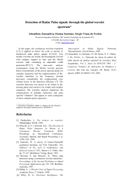
Simetria da DFT
2p k 

X k   xn exp  j
n , k  0,1, N  1
N 

n 0
N 1
2p 

WN  exp  j

N 

N 1
X k   xn WNkn , k  0,1, N  1
n 0
EE-240/2009
2p 

WNk  exp  j
k
N 

N par
N ímpar
EE-240/2009
2
3
fft(x)
1
4
k=0
N=8
7
5
6
WNk  (WNN k )*  X k  X N* k
EE-240/2009
Periodograma
Dada uma seqüência { xn ,
n  0,1, N 1}
| X k |2 , k  0,1, N 1
N  16
 2p k0 
xn  cos
n , k0  2
 N

EE-240/2009
Periodograma
Dada uma seqüência { xn ,
n  0,1, N 1}
| X k |2 , k  0,1, N 1
EE-240/2009
Periodograma
Dada uma seqüência { xn ,
n  0,1, N 1}
| X k |2 , k  0,1, N 1
EE-240/2009
Periodograma
Dada uma seqüência { xn ,
n  0,1, N 1}
| X k |2 , k  0,1, N 1
EE-240/2009
Periodograma
Dada uma seqüência { xn ,
n  0,1, N 1}
| X k |2 , k  0,1, N 1
EE-240/2009
Periodograma
Dada uma seqüência { xn ,
n  0,1, N 1}
| X k |2 , k  0,1, N 1
EE-240/2009
Transformada Inversa
xn = x(nT)
n = 0, ..., N – 1
2p k 

X k   xn exp  j
n , k  0,1, N  1
N 

n 0
N 1
1 N 1
 2p n 
xn   X k exp j
k , n  0,1, N  1
N k 0
 N 
EE-240/2009
Análise Conjunta Tempo-Freqüência
EE-240/2009
Análise Conjunta Tempo-Freqüência
Segmento 1
Segmento 2
DFT
DFT
X k ,1
X k ,2
Segmento 3
DFT
X k ,3
Segmento 4
Segmento 5
DFT
DFT
X k ,4
X k ,5
k  1,, N
EE-240/2009
B = SPECGRAM(A,NFFT,Fs,WINDOW,NOVERLAP) calculates the spectrogram
for the signal in vector A.
SPECGRAM splits the signal into
overlapping segments, windows each with the WINDOW vector and
forms the columns of B with their zero-padded, length NFFT
discrete Fourier transforms. Thus each column of B contains an
estimate of the short-term, time-localized frequency content of
the signal A.
Time increases linearly across the columns of B,
from left to right. Frequency increases linearly down the rows,
starting at 0. If you specify a scalar for WINDOW, SPECGRAM uses a
Hanning window of that length.
WINDOW must have length smaller
than or equal to NFFT and greater than NOVERLAP. NOVERLAP is the
number of samples the sections of A overlap. Fs is the sampling
frequency.
EE-240/2009
Exemplo
Chirp
1
0.5
0
-0.5
-1
CHIRP
Y
0
50
100
150
200
250
300
350
400
Swept-frequency cosine generator.
=
CHIRP(T,F0,T1,F1)
generates
samples
of
a
linear
swept-
frequency signal at the time instances defined in array T.
instantaneous frequency at time 0 is F0 Hertz.
frequency F1 is achieved at time T1.
The
The instantaneous
By default, F0=0, T1=1, and
F1=100.
EE-240/2009
t=0:0.001:2; % 2 secs @ 1kHz sample rate
% Start @ DC, cross 150Hz at t=1sec
x = chirp(t,0,1,150);
specgram(x,256,1000,256,250);
EE-240/2009
Transformada Wavelet
Idéia: Janelas de tamanho variável
"Janelas" largas para
baixa freqüência
(variações de linha de base)
Janelas estreitas componentes
localizados no tempo
(picos estreitos)
EE-240/2009
 a (t ) 
1
t

 
| a |1/ 2  a 
EE-240/2009
 a (t ) 
1
t

 
| a |1/ 2  a 
EE-240/2009
Transformada Wavelet
wav
x
T

(a, b)   x(t ) a*,b (t )dt

Deslocamento
“Onda localizada (b)”:
Média zero e duração limitada (a).
 a ,b (t ) 
Wavelet Mãe
1 t b 


2
|a|  a 
Escala
EE-240/2009
Exemplos de Wavelet:Morlet
 (t )  exp( jt ) exp(0.5t 2 )  [cos(t )  i sen(t )]exp(0.5t 2 )
Real
Real
Imag
Imag
EE-240/2009
Exemplo de Wavelet: Derivada da Gaussiana
 (t ) 
d
exp( 0.5t 2 )  t exp( 0.5t 2 )
dt
EE-240/2009
CWT Real or Complex Continuous 1-D wavelet coefficients.
COEFS
=
CWT(S,SCALES,'wname')
coefficients
of
the
vector
S
computes
the
at
positive
real,
continuous
wavelet
SCALES,
using
wavelet whose name is 'wname'. The signal S is real, the wavelet
can be real or complex.
COEFS = CWT(S,SCALES,'wname','plot') computes
and, in addition, plots the continuous wavelet
transform coefficients.
EE-240/2009
t = 0:0.001:2; % 2 secs @ 1kHz sample rate
% Start @ DC, cross 150Hz at t=1sec
x = chirp(t,0,1,150);
cwt(x,1:64,’gaus1’,’plot’);
EE-240/2009
Exemplo de Aplicação
EE-240/2009
Exemplo de Aplicação
EE-240/2009
Muito Obrigado!
EE-240/2009