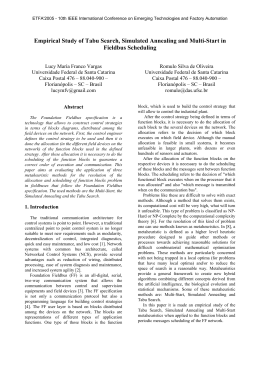
De 25 a 28 de Agosto de 2015.
XLVII
Porto de Galinhas, Pernambuco-PE
SIMPÓSIO BRASILEIRO DE PESQUISA OPERACIONAL
An ILS algorithm for the Robust Coloring Problem
Victor M. R. Silva
Yuri A. M. Frota
Luidi G. Simonetti
Instituto de Computação
Universidade Federal Fluminense
Niterói, RJ, Brazil
[email protected]
[email protected]
[email protected]
RESUMO
Este artigo estuda o Problema da Coloração Robusta (PCR), uma variação do Problema da Coloração Mínima. No PCR, há uma quantidade máxima de cores a ser utilizada em uma
coloração e dois vértices não-adjacentes que possuem a mesma cor são penalizados. A soma das
penalidades da coloração é chamada nível de rigidez. Para resolver o PCR, será apresentado o algoritmo ILS-RCP-RVND, baseado na metaheurística Iterated Local Search (ILS) e que usa a busca
local Random Variable Neighborhood Descent (RVND), além de duas novas estruturas de vizinhança. Os resultados mostram que o algoritmo proposto é competitivo, apresentando resultados
próximos ao ótimo (se existir) ou ao limite inferior.
PALAVRAS CHAVE. Problema da Coloração Robusta. Iterated Local Search. Random
Variable Neighborhood Search.
Área Principal: OC – Otimização Combinatória. MH – Metaheuristicas
ABSTRACT
This paper studies the Robust Coloring Problem (RCP), a variant of the Minimal Coloring Problem which maintains the number of colors fixed. In this problem, two non-adjacent vertex
that have the same color are penalized. The sum of penalties of a coloring is called rigidity level. To
solve the RCP, an Iterated Local Search (ILS) algorithm using the Random Variable Neighborhood
Descent (RVND) local search, called ILS-RCP-RVND, is proposed, as also two new neighborhood
structures. Results shows that the proposed algorithm is competitive, giving results close to the
optimum (if exists) or lower bound.
KEYWORDS. Robust Coloring Problem. Iterated Local Search. Random Variable Neighborhood Search.
Main Area: OC - Combinatorial Optimization. MH - Metaheuristics
2318
De 25 a 28 de Agosto de 2015.
XLVII
Porto de Galinhas, Pernambuco-PE
SIMPÓSIO BRASILEIRO DE PESQUISA OPERACIONAL
1. Introduction
The Minimal Coloring Problem (MCP) has been widely studied in literature and its objective is to minimize the amount of colors used in a graph. The MCP is commonly used to model
many problems whose items can be represented as vertices. A pair of vertices cannot share the
same resource (color) if they are linked by the same edge. As an example of problem which can be
modeled by the MCP are the scheduling problems.
Although, this scheme can be very restrictive to some scheduling problems whose the
resource size to be shared is fixed, making it to appear as a constraint and not as an objective
function to minimize (Yanez and Ramírez, 2003). With this in mind, a new graph coloring problem,
denoted as Robust Coloring Problem (RCP), has been proposed by (Yanez and Ramírez, 2003).
In RCP, adjacent vertices cannot have the same color as in MCP. However, complementary
edges have a penalty in such way that if two vertices of a complementary edge have the same color,
the objective function is increased. The new objective is to find a coloring with a minimal rigidity
level, which is defined as the sum of such penalties. The idea is to minimize the possibility of
including a new edge on the graph that would cause a invalid coloring (Yanez and Ramírez, 2003).
Several applications for the RCP have appeared in literature: timetabling problem, cluster analysis, map coloring (Yanez and Ramírez, 2003), robust aircraft assignment (Lim and Wang,
2005), frequency assignment (Aardal et al., 2007) and any other coloring problem with restricted
resources (Archetti et al., 2014).
2. Problem Definition
Let G = (V, E) be a simple graph, with a set of vertices V = {1, 2, ..., n}, |V | = n,
and a set of edges E, with |E| = m. Let c > 0 be an integer number, and N (c) = {1, 2, ..., c}
a set of colors. A valid c-coloring for the RCP is a C : V → N (c) mapping, with C(i) = C(j),
∀(i, j) ∈ E. A c-coloring exists if and only if c is greater or equal the chromatic number of G, i.e.,
c ≥ χ(G).
The rigidity level R(C) (Yanez and Ramírez, 2003) of a C coloring shows it can be
considered robust in sense that the complementary edges whose equally colored endpoints are penalized, invalidating this coloring if they were added to the graph. A low rigidity level means that
C is more robust. When c = n, we have the minimum rigidity level (R(C) = 0).
Let Ē be the set of complementary edges, with i = j and (i, j) ∈ Ē ⇔ (i, j) ∈ E. Also,
let Ḡ be the complementary graph of G. For each (i, j) ∈ Ē, we have a penalty pij > 0. Figure 1
shows an example of a graph and a valid coloring (for c = 4), with the complementary edges and
their respective penalties. The Figure 1 also shows that in RCP a coloring with less than c colors is
valid.
Figure 1: Example of coloring C. R(C) = 9
2319
De 25 a 28 de Agosto de 2015.
XLVII
Porto de Galinhas, Pernambuco-PE
SIMPÓSIO BRASILEIRO DE PESQUISA OPERACIONAL
In order to find the best coloring possible, (Yanez and Ramírez, 2003) introduced a binary
programming model. Let xik be a decision variable defined by xik = 1 if C(i) = k, and xik = 0
otherwise. Also, let yij , (i, j) ∈ Ē, be an auxiliary variable defined by yij = 1 if exists a k ∈
{1, ..., c} | xik = xjk = 1, and yij = 0 otherwise.
Hence, the RCP can be stated as (Yanez and Ramírez, 2003):
pij yij
(1)
P CR = min
(i,j)∈Ē
s.a.
c
xik = 1, ∀ i ∈ V
(2)
k=1
xik + xjk ≤ 1, ∀ (i, j) ∈ E, ∀ k ∈ {1, ..., c}
(3)
xik + xjk − 1 ≤ yij , ∀ (i, j) ∈ Ē, ∀ k ∈ {1, ..., c}
(4)
x ∈ {0, 1}
|V |
e y ∈ {0, 1}
|Ē|
(5)
The first and second constraint groups assure that each vertex must be assigned to exactly
one color and two vertices linked by an edge cannot have the same color. The third constraint
assigns the value yij = 1 to each pair of non-adjacent vertices with the same color. The last
constraint group imposes binary constraint to the variables.
The authors state that this formulation can only solve small or medium size problems
(Yanez and Ramírez, 2003). They also prove that the RCP is NP-hard, which states that for high size
instances some heuristics should be applied. Some algorithms have been proposed to solve the RCP,
such as Genetic Algorithm (Yanez and Ramírez, 2003; Wang and Xu, 2013), Simulated Annealing
(Lim and Wang, 2005; Gutierrez-Andrade M.A., 2007; Wang and Xu, 2013), Tabu Search (Lim and
Wang, 2005; Gutiérrez-Andrade et al., 2011; Wang and Xu, 2013), Scatter Search (Lara-Velázquez
et al., 2005), GRASP (Gutiérrez-Andrade et al., 2011), Ant Colony (Laureano-Cruces et al., 2011)
and Hill Climbing (Wang and Xu, 2013).
In order to solve the RCP exactly, two algorithms have been proposed. (Yanez and
Ramírez, 2003) proposed a binary programming model, which could solve only small instances.
(Archetti et al., 2014) proposed a set covering formulation, which could solve small and large size
instances.
3. Proposed Algorithm
In this paper, we propose a new algorithm, based on the Iterated Local Search (ILS)
metaheuristic (Lourenço et al., 2002). This metaheuristic is based on the idea of improving the
local search procedure by providing a new start from a perturbation of the current solution, as
shown in the Algorithm 1.
Algorithm 1 ILS(maxIter)
1: s = GenerateInitialSolution
2: s∗ = LocalSearch(s)
3: while stopCriteria do
4:
s = Perturbation(s*)
5:
s∗ = LocalSearch(s’)
6:
s∗ = AcceptanceCriterion(s*,s*’)
7: end while
The perturbation phase makes the algorithm explore the solution space, making it possible to converge for a global optimum. The perturbation mechanism is very important for the ILS.
It cannot be too small or too big. If it is too small, the solution may not escape of actual local
2320
XLVII
De 25 a 28 de Agosto de 2015.
Porto de Galinhas, Pernambuco-PE
SIMPÓSIO BRASILEIRO DE PESQUISA OPERACIONAL
optimum. If it is too big, the solution can become completely aleatory.
3.1. Neighborhoods and Local Search
The neighborhood structures for the RCP are categorized by changing the colors of the
vertex. In this work, we used 4 structures. Two of these instances can add colors that were not used
in the current coloring and the other two try to rearrange the colors. The complexity to recalculate
the cost of a new coloring is O(n), as shown by (Wang and Xu, 2013).
The neighborhood structures used are presented below:
• SVR (Single Vertex Recoloring), proposed by (Wang and Xu, 2013), which consists in one
single change of color for a randomly vertex, a set of r vertex (called Random Single Vertex
Recoloring - RSVR) or all vertex (called Enumerative Single Vertex Recoloring - ESVR). The
new coloring in the RSVR and ESVR neighborhood will be the one that have the smallest
total penalty. The complexity of this structure is O(cn) for the SVR, O(rcn) for the RSVR
and O(n2 c) for the ESVR.
• MVR (Multi Vertex Recoloring), a new neighborhood structure based on the SVR neighborhood, consists in changing the color of all vertex in a set of α vertex (α ∈ {1, .., v}). All
colors are tested for each vertex of the set and more than one color can be modified. The
complexity of structure is O(cα .αn), and it is described in the Algorithm 2;
Algorithm 2 MVR(α)
1: L = list of α vertex in V
2: C = every coloring possible for G with every combination of colors for all L vertex
3: pbest = ∞
4: for each Ci in C do
5:
p = penalty(Ci )
6:
if p < pbest then
7:
C∗ = Ci
8:
pbest = p
9:
end if
10: end for
11: return C∗
• IG-K*-cycle (Improvement Graph Based K*-cycle), proposed by (Wang and Xu, 2013),
which creates an improvement graph and then creates up to θ cycles of improvement with
a maximum K vertex, trying to change the colors of the vertex at each cycle. The complexity
of this structure is O(Kn2 θ), as shown by the authors;
• ΘK-cycle, a new neighborhood based on the IG-K*-cycle, which consists in: (i) a cycle with
the first vertex of the list is created; (ii) create cycles of size j = 2 to K based upon the best
cycle found in iteration j − 1, with the next vertex of the list in each possible position of the
best cycle; (iii) search the best cycle of this iteration (the one with lower penalty); (iv) if the
best cycle found with size j is the best cycle found so far then update the best cycle. This
process is made Θ times and then we return the best cycle, changing the color of each vertex
i with the color of vertex i − 1. The complexity of structure is O(Kn2 Θ), and it is described
in the Algorithm 3;
Random Variable Neighborhood Descent (RVND) (Penna et al., 2013) is a local search
method which consists in exhaustively explore a set of feasible solutions for each neighborhood
2321
De 25 a 28 de Agosto de 2015.
XLVII
Porto de Galinhas, Pernambuco-PE
SIMPÓSIO BRASILEIRO DE PESQUISA OPERACIONAL
Algorithm 3 ΘK-cycle(k, Θ)
cyclebest = ∅
pbest = ∞
for i = 1 to Θ do
vertex = list of K random vertex
cyclesize [1] = vertex[1]
for j = 2 to K do
cycles = every cycle with vertex[j] in each position 1,..,j in cyclesize [j-1]
psize = ∞
for each c in cycles do
penalty = w(c)
if penalty < psize then
psize = penalty
cyclesize [j] = c
if penalty < pbest then
pbest = penalty
cyclebest = c
end if
end if
end for
end for
end for
return cyclebest
N (s), starting from an initial solution s. In RVND classical version, we sort the sequence of
neighborhood structures, generating a set of neighborhood structures N = Ni , i ∈ {1, .., n}. If the
best neighbor of the first selected neighborhood structure Nr (s) is worse than the solution s, we
move to the next neighborhood Nr+1 (s), until we reach the last neighborhood. If not, we sort again
the set of neighborhood structure, and restart the process, as shown in Algorithm 4.
3.2. Initial Solution
The mechanism to create an initial solution consists in allocate a random color to each
vertex. This method can create invalid colorings, which are going to be accepted with an elevated
cost. When all vertex are associated with a color, we define a random list of them and apply the SVR
neighborhood for each vertex, in order to select a new color that will generate a better coloring. We
call this method Refined Initial Solution (RIS), and it is described in Algorithm 5.
3.3. Cost Function and Acceptance Criteria
Sometimes during execution, due to the problem complexity, it is hard for an algorithm to
walk only by valid solutions. Thus, inviable solutions will be accepted by the ILS-RCP-RVND, but
with his rigidity level highly penalized. The new rigidity function R̄(C) is defined by:
R̄(C) =
(i,j)∈Ē
pij yij +
μȳij
(6)
(i,j)∈E
In which:
• yij = 1 if vertices i and j ∈ Ē and have different colors; 0 otherwise
• pij is the cost of complementary edge (i, j) ∈ Ē
2322
XLVII
De 25 a 28 de Agosto de 2015.
Porto de Galinhas, Pernambuco-PE
SIMPÓSIO BRASILEIRO DE PESQUISA OPERACIONAL
Algorithm 4 RVND(s)
1: N = sorted set of neighborhood structures
2: while improvement do
3:
i=1
4:
while i < n do
5:
s’ = best neighbor of neighborhood Ni (s)
6:
if f (s ) < f (s) then
7:
s’ = ESVR(s’)
8:
s = s’
9:
i=1
10:
N = sorted set of neighborhood structures
11:
else
12:
i++
13:
end if
14:
end while
15: end while
• ȳij = 1 if vertex i and j ∈ E and have the same color; 0 otherwise
• μ is the penalty of two vertex having the same color
The value of μ is dynamically defined by the algorithm. At each iteration, if the new
solution is viable, the value of μ is decreased by δ% of its original value, until a certain limit. Else,
is increased by μ% of its original value, until a certain limit. This process prioritizes neighbor
solutions that have more valid neighbors, decreasing the penalty for invalid solutions.
Our acceptance criteria between a solution s and a new solution s’ will be when s’ has a
lower rigidity level than s. In other words, when the value of the cost function of s’ is lower than s.
3.4. ILS-RCP-RVND
The ILS-RCP-RVND algorithm has some differences from the algorithm presented in Algorithm 1. We use a multi-start mechanism in order to generate a set of initial solutions. We also use
a perturbation method by level which consists of: at each level, we have maxIter iterations. If we
cannot obtain a better solution in maxIter iterations, we will increase one level until maxLevel.
If a better solution is reached, the level and iteration will be restarted to the initial value. For each
iteration, the algorithm randomly chooses 2+level vertex and gives to each vertex a new random
color. The stop criteria is when the algorithm reaches maxLevel.
The ILS-RCP-RVND algorithm is presented in Algorithm 6.
Algorithm 5 RIS
1: C = NULL
2: for each v in V do
3:
C(v) = random color between the c colors
4: end for
5: L = random list of V vertex
6: for each v in L do
7:
C = SRV (C, v)
8: end for
9: return C
2323
XLVII
De 25 a 28 de Agosto de 2015.
Porto de Galinhas, Pernambuco-PE
SIMPÓSIO BRASILEIRO DE PESQUISA OPERACIONAL
Algorithm 6 ILS-RCP-RVND
1: sbest = NULL
2: originalμ = 100000
3: for start=1 to maxMultiStart do
4:
μ = originalμ
5:
s = RIS()
6:
s = RVND(s)
7:
for level = 1 to maxLevel do
8:
for iter = 1 to maxIter do
9:
s’ = s
10:
for i = 1 to 2 + level do
11:
select a vertex v randomly
12:
assign a new color to v randomly
13:
update s’
14:
end for
15:
s’ = RVND(s’)
16:
if isViable(s’) then
17:
μ = μ − δ ∗ originalμ
18:
else
19:
μ = μ + δ ∗ originalμ
20:
end if
21:
if AcceptanceCriteria(s’,s) then
22:
s = s’
23:
iter = 1
24:
level = 1
25:
else
26:
iter++
27:
end if
28:
end for
29:
level++
30:
end for
31:
if AcceptanceCriteria(s,sbest ) then
32:
sbest = s
33:
end if
34: end for
35: return sbest
2324
De 25 a 28 de Agosto de 2015.
XLVII
Porto de Galinhas, Pernambuco-PE
SIMPÓSIO BRASILEIRO DE PESQUISA OPERACIONAL
4. Computational Results
4.1. Instances
In the experiment were used 56 instances divided in five sets: three were created using
the technique described in (Yanez and Ramírez, 2003) and presented in (Archetti et al., 2014), and
two were adapted from DIMACS instances (Johnson and Trick, 1996). The optimum value of some
instances is not known, but they have a lower bound (Archetti et al., 2014). These values, although
sometimes are not optimum, are close to it (the upper and lower bounds have little gap) and were
used as reference by our experiment.
Table 1 shows the configuration of each set of instances. In this table, Set denotes the
name of the set, v denotes the interval of vertex, k denotes the interval of colors and Qty denotes
the amount of instances in the set.
Table 1: Instances
Set
DIM ACS1
DIM ACS2
Archetti40
Archetti90
Archetti120
v
{11..128}
{11..128}
{40}
{90}
{120}
k
{6..110}
{8..84}
{14, 15}
{30, 31}
{40, 41}
Qty
14
17
5
10
10
4.2. Experimental Design and Results
The ILS-RCP-RVND algorithm was executed 5 times for each instance shown in Table 1
with the following parameters, chosen empirically:
• Size of set r of RSVR: 3
• Size of set α of MVR: 2
• Maximum size of IG-K*-cycle’s set k of vertex: 5
• Maximum size of IG-K*-cycle’s candidate list θ: 100
• Size K of ΘK-cycle list of vertex: 5
• Quantity of cycles Θ produced in ΘK-cycle: 10
• Multi-start maxM ultiStart for the ILS-RCP: 5
• Levels maxLevel for the ILS-RCP: 3
• Iterations maxIter by level for the ILS-RCP: 30
• Penalty μfor invalid solutions: 10000
• Adjust of the penalty δ for μ: 20
The ILS-RCP-RVND was implemented in C++ and all experiments were carried out on
an Intel Core 2 Duo E7500, 2.93GHz machine with 1.98 GB of RAM. The time limit was set to
7200 seconds for each execution.
To measure the quality of the proposed algorithm, a comparison was made between the
results found in ILS-RCP-RVND and the Branch-and-Price (B-P) proposed by (Archetti et al., 2014)
(which is also the lower bound for our set of instances). The results for each set are in Table 2, where
is demonstrated the mean gap between the solution found for ILS-RCP-RVND and the reference
2325
De 25 a 28 de Agosto de 2015.
XLVII
Porto de Galinhas, Pernambuco-PE
SIMPÓSIO BRASILEIRO DE PESQUISA OPERACIONAL
value of the instances of that set and the mean coefficient of variance (CV) (the ratio of the standard
variation to the mean) of the instances of each set. The instances and detailed results for each set
are available with the authors1
Table 2: Results for each set
Set
DIM ACS1
DIM ACS2
Archetti40
Archetti90
Archetti120
GAP (%)
0.02
0.03
0.39
1.34
2.30
CV (%)
0.21
0.53
1.28
3.51
8.21
4.3. Result Analysis
As seen on Table 2, tests with ILS-RCP-RVND had little gap and the coefficient of variance was considerably low. In sets Archetti90 and Archetti120 we have a greater variance (8.21%),
but with a relatively low gap (2.3%) for reference results.
ILS-RCP-RVND stayed in the limits of resources and time except for one instance, even
with the amount of complex neighborhood structures inside the algorithm.
In overall, mean gaps and CV for the instances were rather low when compared to the
Branch-and-Price, which indicates that ILS-RCP-RVND is efficient (because of low gaps) and robust (because of low CV).
5. Conclusions
This study main contribution is the algorithm development and the new neighborhood
structures for the RCP. We believe that the neighborhood structures presented in this paper can
be used in algorithms for the classical Coloring Problem. Our experimental results show that the
proposed algorithm can be very efficient and robust, even in challenging sets of instances. In comparison to the Branch-and-Price algorithm for the RCP, the ILS-RCP-RVND algorithm can reach
results close to the optimum, with a lower time.
References
Aardal, K. I., Hoesel, S. P. M. V., Koster, A. M. C. A., Mannino, C., and Sassano, A. (2007).
Models and solution techniques for frequency assignment problems. In Annals of Operations
Research, volume 153, pages 79–129.
Archetti, C., Bianchessi, N., and Hertz, A. (2014). A branch-and-price algorithm for the robust
graph coloring problem. Discrete Applied Mathematics, 165:49–59.
Gutiérrez-Andrade, M. A., Lara-Velázquez, P., López-Bracho, R., and Ramírez-Rodríguez, J.
(2011). Heuristic for the robust coloring problem. Revista de Matemática: Teoría y Aplicaciones,
18(1):137–147.
Gutierrez-Andrade M.A., Lara-Velazquez P., d. l. C. S. S. (2007). A new simulated annealing algorithm for the robust coloring problem. Journal of Industrial Engineering International,
3(5):27–32.
Johnson, D. J. and Trick, M. A. (1996). Cliques, Coloring, and Satisfiability: Second DIMACS
Implementation Challenge, Workshop, October 11-13, 1993. American Mathematical Society,
Boston, MA, USA.
Lara-Velázquez, P., Gutiérrez-Andrade, M. A., Ramírez-Rodríguez, J., and López-Bracho,
R. (2005). Un algoritmo evolutivo para resolver el problema de coloración robusta. Revista de
Matemática: Teoría y Aplicaciones, 12(1-2).
1
http://www.vmrs.com.br/sbpo2015/results.pdf
2326
XLVII
De 25 a 28 de Agosto de 2015.
Porto de Galinhas, Pernambuco-PE
SIMPÓSIO BRASILEIRO DE PESQUISA OPERACIONAL
Laureano-Cruces, A. L., Ramírez-Rodríguez, J., Hernández-González, D. E., and MéndezGurrola, I. I. (2011). An ant algorithm for the robust coloring problem. In ICGST Conference
on Artificial Intelligence and Machine Learning, AIML-11 Dubai-11 Conference, pages 57–60.
ICGST.
Lim, A. and Wang, F. (2005). Robust graph coloring for uncertain supply chain management. In
HICSS ’05. Proceedings of the 38th Annual Hawaii International Conference on System Sciences,
2005. IEEE Computer Society.
Lourenço, H. R., Martin, O. C., and Stützle, T. (2002). Handbook of Metaheuristics, chapter
Iterated Local Search, pages 321–353. Kluwer Academic Publishers, Norwell, MA.
Penna, P. H. V., Subramanian, A., and Ochi, L. S. (2013). An iterated local search heuristic for
the heterogeneous fleet vehicle routing problem. Journal of Heuristics, 19(2):201–232.
Wang, F. and Xu, Z. (2013). Metaheuristics for robust graph coloring. Journal of Heuristics,
19:529–548.
Yanez, J. and Ramírez, J. (2003). The robust coloring problem. European Journal of Operational
Research, 148(3):546–558.
2327