DOI: 10.5433/1679-0359.2012v33Supl1p2959 Study of a parallel algorithm in liquid front propagation for Ceará’s soils using the finite difference method1 Estudo de um algorítmo paralelo em frentes de propagação líquidas para solos do Ceará usando o método de diferenças finitas Paulo Alexandre Costa Rocha2*; Daniel Albiero3; Maria Eugênia Vieira da Silva2; Ernesto da Silva Pitombeira4 Abstract This work presents a numerical model to simulate the propagation of a liquid front in unsaturated soils. The governing flow equations were discretized using centered finite differences for the space coordinate and backward differences for the time coordinate. The generated scheme is fully implicit, but “lagging the non-linearities” as referred to the determination of the soil characteristic properties as function of the hydraulic head. The soil properties, moisture content and the unsaturated hydraulic conductivity, were curve fitted for two types of soil (Alluvial Eutrophic and Red-Yellow Podsol) found in the Northeast region of Brazil. The results show that the Alluvial Eutrophic liquid front diffuses faster than the RedYellow Podsol front. The use of a parallel algorithm showed that it can be indicated for bigger problems (2-D), where the processing speed gain can reach values between 2-3 times, against simple problems (1-D). Key words: Groundwater, Richards’ equation, numerical simulation, speed up Resumo Este trabalho apresenta um modelo numérico para simular a propagação de uma frente de onda líquida em solos insaturados. As equações de governo do fluxo de água foram discretizadas usando o método das diferenças finitas centradas para as coordenadas de espaço e diferenças atrasadas para a coordenada de tempo. O esquema gerado é completamente implícito, mas as “influências das não linearidades” foram referidas na determinação das propriedades características do solo como função do recalque hidráulico. As propriedades do solo, teor de água e condutividade hidráulica insaturada foram representadas por curvas de regressão para dois tipos de solos (Aluvial Eutrófico e Podzólico Vermelho Amarelo) normalmente encontrados na região Nordeste do Brasil. Os resultados mostraram que a frente de onda do solo Aluvial Eutrófico difunde-se mais rápido do que o solo Podzólico Vermelho Amarelo. O uso do algoritmo paralelo mostrou-se adequado a grandes problemas na simulação 2-D, onde a velocidade de processamento pode alcançar valores entre 2-3 vezes maiores do que problemas simples (1-D). Palavras-chave: Equações de richards, simulação numérica, águas subterrâneas Post Graduate Program in Mechanical Engineering. Federal University of Ceará, UFC, Technological Centre, Department of Mechanical Engineering, Av. Mister Hull, 2977, Campus do Pici, Bloco 714, Zip Code: 60455-760, Fortaleza, CE, Brazil. 2 Profs. of Mechanical Engineering, UFC, Fortaleza, CE, Brazil. E-mail: [email protected]; [email protected] 3 Prof. of Agricultural Engineering, UFC, Fortaleza, CE, Brazil. E-mail: [email protected] 4 Prof. of Water Resources, UFC, Fortaleza, CE, Brazil. E-mail: [email protected] * Author for corespondence 1 Recebido para publicação 03/05/12 Aprovado em 09/10/12 Semina: Ciências Agrárias, Londrina, v. 33, suplemento 1, p. 2959-2972, 2012 2959 Rocha, P. A. C. et al. Introduction The study of infiltration processes is very important in many technological and environmental applications, particularly in water resources research, in the determination of liquid fronts propagation in soils. The literature in this area is very wide (ZACHMANN, 1978; ZACHMANN; DUCHATEAU; KLUTE, 1981; ROSS, 1990; CELIA; BOULOUTAS, 1990). The knowledge of the behavior of a water front propagation in unsaturated soils helps on the rational planning of the water reserves use, e.g. in irrigation systems and in raining areas. Another example of an infiltration process is the spill of a liquid contaminant on unsaturated porous surfaces that can cause many kinds of ecological problems, particularly if the liquid front reaches any underground aquifer. The determination of the contaminating propagation can avoid larger environmental injuries and help the recuperation of the region. The prediction of groundwater flow and contaminant transport from mathematical models deals with considerable uncertainty due to the presence of heterogeneities in natural soil formations (Aguire and Highighi, 2002). The principles of continuity of mass and momentum or energy may be applied to describe overland flow conditions in surface irrigation systems (SHAYYA; BRALTS; SEGERLIND, 1993). The understanding of hydrological processes at watershed scale is an important task in order to optimize management of the available surface water and groundwater resources, mainly the mechanisms overland flow and perched zones of saturated soil and regolith water (NUÑES-GONZALEZ et al., 2011). If the determination of the liquid front propagation as a function of the space coordinates and time is desired, the mass and momentum conservation equations for an infinitesimal control volume of the flow (for a study of a one dimensional finite difference implicit scheme, see Johnsen (1992)) need to be solved. The partial differential equation for the pressure head as a function of the spatial coordinates and time, commonly known as the Richards Equation, which express the mass and momentum balances, needs information about the specific characteristics of the soil. The soil can be characterized using experimental expressions based on field measures to estimate the moisture content and the hydraulic conductivity, as a function of the pressure head. We also have to define proper boundary and initial conditions for the solution of the system. Recent interests in unsaturated flow has shifted to the determination of the velocity (specific discharge or flux) in the unsaturated soil because it was realized that this zone acts as a buffer for contaminants that eventually move to the ground water table (MISRA; NIEBER, 2004). The partial differential equation that describes the system is parabolic, of second order, and non linear. And a general analytical solution is not available, except for specific cases, where the equations for the hydraulic conductivity and the moisture content are constant or expressed as special functions (ZACHMANN, 1978). Accurate and efficient numerical wave approximation is important in many areas of study as liquid front waves, and finite difference methods have the advantage of ease of use as well as high order convergence, but often require a uniform grid, and stable boundary closure can be non-trivial (FERNANDO; HU, 2011). This work presents a numerical model to determinate the propagation of a water front, in unsteady-state flow in a unsaturated soil, using finite differences to discretize the domain. The program developed includes information about two kind of Ceará’s soils: The Alluvial Eutrophic and the Red-Yellow Podsol, which have experimental data published in the literature about hydraulic conductivity (BEZERRA, 1998; CORDEIRO, 2960 Semina: Ciências Agrárias, Londrina, v. 33, suplemento 1, p. 2959-2972, 2012 Study of a parallel algorithm in liquid front propagation for Ceará’s soils using the finite difference method 1998) and moisture content (D’ÁVILA, 1983; BEZERRA, 1985; SAUNDERS, 1990; FERREIRA, 1990; GOMES FILHO, 1991), commonly known as the characteristic curve. The parallel algorithm was developed in a modular way to easily permit the application of another kind of soils. It was used both in one and two dimensional cases, to permit a comparison of processing speed gains. were used a posteriori in the numerical resolution of the Richards equation. For the two soils studied (Alluvial Eutrophic and Red-Yellow Podsol), these characteristic curves were fitted using the Van Genuchten (1980) model as, θ = C1 + Soils data and characteristics curves [1 + (C .ψ ) ] C5 C 6 (1) 4 Material and methods This work was developed in two parts. In the first, a literature search on the experimental data for the moisture content (q) as a function of the pressure head (y), and the hydraulic conductivity (K) as a function of the moisture content (q) was carried out. These data were then statistically studied, and the procedure is presented in the next section. The second part presents the discretization of the Richards equation in both one and two dimensions, using centered finite differences for the spatial derivatives and forward differences for the time derivative, to obtain a fully implicit scheme. This scheme generated a system of equations equivalent to the number of discrete points in the domain, which was solved for the one and two dimensional cases. To carry out the computational work, parallel routines were introduced in the program, basically in three stages: The determination of the initial and boundary conditions, the creation of the linear system of equations and finally its resolution. The processing times were then measured for a different number of processors. C 2 − C3 where C1, C2, C3, C4, C5 e C6 are constants determined in the adjust of the experimental curves. The hydraulic conductivity (K) data as a function of the soil moisture content (q) were used in a non linear exponential regression to fit the curves and find a relationship between the hydraulic conductivity (K) and the pressure head (y) for the two soils in study. Description and discretization of the problem Using the mass and momentum conservation laws in an infinitesimal control volume, the liquid flow in an unsaturated media, the Richards equation, is presented (ZACHMANN; DUCHATEAU; KLUTE, 1981; CELIA; BOULOUTAS, 1990; ROSS, 1990) as, K z 1 C z t z 1 C K z z z t ( 2 ) (2) (2) 1 C K x K z t x x z z 1 C K x K z x x z t (3) z applied. This model relate where the Darcy’s model was where the Darcy’s model was applied. This model relates the liquid flow As already mentioned, the experimental data conductivity and the gradient of hydraulic head as conductivity and the gradient of hydraulic head as used to characterize the soil were obtained from whereqthe Darcy’s K (hmodel z ) was applied. This( 4model ) q Kthe (liquid h z ) flow with its hydraulic ( 4 ) conductivity the literature published by local authors. The relates The expressions (2) head and as (3) are second order parabol theexpressions gradient of(2)hydraulic and (3) are second order parabolic partial differe characteristic curves for the both studied soils are andThe hydraulic conductivity moisture content used, expressions eq presented in the results section. hydraulic conductivity equationsused, (2) and qand = moisture − K∇and ⋅ (hcontent − z ) expressions (4) no analytical Two boundary Dirichletconditions boundary and an no analytical solution.solution. Two Dirichlet andconditions an initial condition The experimental data were curve fitted, using dimensional case, these conditions are, dimensional case, these conditions are, non linear regression. The expressions obtained (z,0) =(z,0) 0, = , 0 < z < zL 0 < z < z( 5 ) 0 L 2961 = 1, 1, p. 2959-2972, 2012 Semina: Ciências Agrárias, Londrina, v. 33,(0,t) suplemento (0,t) = 1, (zL,t) = L, (zL,t) = L, t>0 t>0 (6) ( ( Rocha, P. A. C. et al. The expressions (2) and (3) are second order parabolic partial differential equations. For the hydraulic conductivity and moisture content expressions used, equations (2) and (3) are nonlinear, with no analytical solution. Two Dirichlet boundary conditions and an initial condition were used. For the one dimensional case, these conditions are, y(z,0) = y0, 0 < z < zL (5) ) t > 0 (6) ψ i j +1 −ψ i j−+11 ⋅ ∆t + K i −j 1 / 2 ⋅ ∆t ∆z ψ j +1 −ψ i j +1 + K i +j 1 / 2 ⋅ i +1 ⋅ ∆t − K i +j 1 / 2 ⋅ ∆t ∆z (10) for the one dimension case and ( )( ) C ψ mj ,i ⋅ ψ mj +,i1 −ψ mj ,i ⋅ ∆z ⋅ ∆x = − K mj ,i −1 / 2 ⋅ + K mj ,i +1 / 2 ⋅ + K mj +1 / 2,i ⋅ y(0,t) = y1, y(zL,t) = yL, ( )( C ψ i j ⋅ ψ i j +1 − ψ i j ⋅ ∆z = − K i −j 1 / 2 ⋅ −K j m −1 / 2 ,i ⋅ ψ mj +,i1 −ψ mj +,i1−1 ψ j +1 m ,i +1 ψ j +1 m +1,i ∆z −ψ mj +,i1 ∆z −ψ mj +,i1 ∆x ψ mj +,i1 −ψ mj +−11,i ∆x ⋅ ∆x ⋅ ∆t + K mj ,i −1 / 2 ⋅ ∆x ⋅ ∆t ⋅ ∆x ⋅ ∆t − K mj ,i +1 / 2 ⋅ ∆x ⋅ ∆t (11) ⋅ ∆z ⋅ ∆t ⋅ ∆z ⋅ ∆t for the two-dimensional case. where for the numerical simulation, the values y0 = –61,5 cm, y1 = –20,7 cm, yL = –61,5 cm and zL = 100 cm were used. Four Dirichlet conditions, and one initial, were used for the two-dimensional case, y(x,z,0) = y0, 0 < x < xL, 0 < z < zL Subroutine a: definition of the boundary and initial conditions; (8) Subroutine b: construction of the linear system, which generates one equation per domain point. Since the soil’s properties depend upon the pressure head at that instant of time, which are not known, the values of (y) used were from the previous instant (lagging in time solution); y(x,0,t) = yfilm, 0,4.xL ≤ x ≤ 0,6.xL y(x,0,t) = yx0, 0 < x < 0,4.xL, 0,6.xL < x < xL y(x,zL,t) = yxL, t > 0, 0 < x < xL The algorithm developed to solve both problems (one and two dimensions) consisted basically of three subroutines, for each different instant of time: (7) y(0,z,t) = y0z, y(xL,z,t) = yLz, t > 0, 0 < z < zL Numerical solution (9) where the values y0 = –61,5 cm, y0z = –61,5 cm, yLz = –61,5 cm, yfilm = –20,7 cm, yx0 = –61,5 cm, yxL = –61,5 cm, xL = 100 cm and zL = 100 cm were used in the numerical calculation. The discretization of the Richards equation was made by centered finite differences for the spatial derivatives and forward differences for the time derivative. The application of these differences on the continuous equations resulted in a fully implicit scheme, and the correspondent discretized forms of (2) and (3) are, Subroutine c: the numerical resolution of the linear system. This algorithm generated a FORTRAN code which solved the one and two dimensional problems. Results and Discussion Characteristic curves The following figures 1(a) and 1 (b) presents the characteristic curves for the two soils studied using the experimental data. 2962 Semina: Ciências Agrárias, Londrina, v. 33, suplemento 1, p. 2959-2972, 2012 Study of a parallel algorithm in liquid front propagation for Ceará’s soils using the finite difference method Figure 1. (a) Non linear curve fit for the characteristic curve of the Alluvial Eutrophic soil. Data: Ferreira Figure(b) 1. Non (a) Non linear curvefitfitfor forthe the characteristic characteristic curve Alluvial Eutrophic soil. Data: Ferreira (1990), (b) (1990), linear curve curveofofthethe Red-Yellow Podsol soil. Data:Gomes Filho Non linear curve fit for the characteristic curve of the Red-Yellow Podsol soil. Data:Gomes Filho (1991). (1991). Model: Van Genuchten 0.50 2 0.45 (cm3/cm3) 0.40 0.35 R = 0.95629 P1 P2 P3 P4 P5 P6 0.10448 1.17723 0.82277 0.0018 0.86538 1.60409 0.30 (a) 0.25 0.20 0.15 0.10 10 100 1000 (-cm H2 O) 0.35 Model: Van Genuchten 2 0.30 = 0.93416 P1 P2 P3 P4 P5 P6 0.04451 1.12662 0.87338 0.00844 1.94977 0.9134 0.20 3 3 (cm /cm ) 0.25 R 0.15 (b) 0.10 0.05 0.00 10 100 1000 (-cm H2O) Source: Elaboration of the authors. Source: Elaboration of the authors. Hydraulic Condutivity (K) versus soil Moisture Content () 2963 The hydraulic conductivity coefficient (K) versus the soil moisture content2012 () data was treated in Semina: Ciências Agrárias, Londrina, v. 33, suplemento 1, p. 2959-2972, an analogous way. Using the same criteria as in the previous section, the works of El-Husny (1979) for the Rocha, P. A. C. et al. Hydraulic Condutivity (K) versus soil Moisture Content (q) The hydraulic conductivity coefficient (K) versus the soil moisture content (q) data was treated in an analogous way. Using the same criteria as in the previous section, the works of El-Husny (1979) for the Alluvial Eutrophic soil and Bezerra (1998), for the Red-Yellow Podsol soil were used. The non linear regression model is an exponential growth, which generated the graphs on the Figures 2a and 2b, as well as the following expressions: For the Alluvial Eutrophic soil (Figure 2(a)), K (θ ) = 0,00003.eθ / 0, 0433 (12) and for the Red-Yellow Podsol soil (Figure 2(b)), K (θ ) = 2,0213E − 8.eθ / 0, 01648 As a result of the previous non linear regression, with pressure head values expressed in cm, the following expressions shown were obtained: For the Alluvial Eutrophic soil (Figure 3 a), θ = 0,10448 + 1,17723 − 0,82277 [1 + (0,0018.ψ ) ] 0 ,86538 1, 60409 (14) For the Red-Yellow Podsol soil (Figure 3 b), θ = 0,04451 + 1,12662 − 0,87338 [1 + (0,00844.ψ ) ] 1, 94977 0 , 91134 (15) It can be seen that the Alluvial soil retains more moisture than the Red-Yellow Podsol, for equal pressure head values. Even using data from different depths, the curve fit is good, what justifies the use of only one expression for all depths. (13) Propagation – one dimensional model It is concluded that the hydraulic conductivity in the Alluvial Eutrophic soil is higher than in the Red-Yellow Podsol soil, in the range of values used as boundary and initial conditions, what will lead to a faster liquid propagation in the first case. It is important to say that the hydraulic conductivity units were converted to SI in equations (10) and (11), once the primary obtained values were in cm/ day, as can be seen in Figure 2. The propagation of the liquid front was simulated, using the discretized form of Richards equation (10) as well as equations (12), (13), (14) and (15). The results show the pressure head profiles (y) as a function of the depth (z), for the two soils in study, in several instants of time (1 s, 10 s, 100 s, 1.000 s, 10.000 s, 100.000 s and 200.000 s) as seen in Figures 3(a) and 3(b). The curve fit was not so good for the Alluvial soil, as it was for the Red-Yellow Podsol soil, showing a variability of the properties as the depth changes. 2964 Semina: Ciências Agrárias, Londrina, v. 33, suplemento 1, p. 2959-2972, 2012 and for the Red-Yellow Podsol soil (Figure 2(b)), K ( ) 2,0213E 8.e / 0,01648 ( 13 ) Study of a parallel algorithm in liquid front propagation for Ceará’s soils using the finite difference method Figure 2. (a) Non linear regression graph for the Alluvial Euthophic K(q). Data: El-Husny (1979), (b) Non linear Figure 2. (a) Non regressionPodsol graphK(q). for the Alluvial K(). Data: El-Husny (1979), (b) Non regression graph forlinear the Red-Yellow Data: Bezerra Euthophic (1998). linear regression graph for the Red-Yellow Podsol K(). Data: Bezerra (1998). K( ) (cm/day) Model: ExpGro1 2.5 R^2 = 0.25652 2.0 y0 A1 t1 0 0.00003 0.0433 1.5 (a) 1.0 0.5 0.0 0.28 0.30 0.32 0.34 0.36 0.38 0.40 0.42 0.44 0.46 0.48 0.50 (cm3/cm3) 3000 K() (cm/day) Model : ExpGro1 2500 R^2 = 0.97717 2000 y0 A1 t1 0 2.0213E-8 0.01648 1500 (b) 1000 500 0 0.30 0.32 0.34 0.36 3 0.38 0.40 0.42 0.44 3 (cm /cm ) Source: Elaboration of the authors. 2965 Semina: Ciências Agrárias, Londrina, v. 33, suplemento 1, p. 2959-2972, 2012 Rocha, P. A. C. et al. Figure 3. (a) Simulation results of the liquid front propagation for the Alluvial Eutrophic soil with time, (b) Simulation Figure 3. (a) Simulation results of the liquid front propagation for the Alluvial Eutrophic soil with time, (b) results of the liquid front propagation forpropagation the Red-Yellow Podsol soil withPodsol time. soil with time. Simulation results of the liquid front for the Red-Yellow pressure head (cm H2O) Alluvial - 1s Alluvial - 10s Alluvial - 100s Alluvial - 1.000s Alluvial - 10.000s Alluvial - 100.000s Alluvial - 200.000s 0 -10 -20 (a) -30 -40 -50 -60 -70 pressure head (cm H2O) 0 20 40 60 80 100 depth (z) 0 -10 -20 -30 -40 (b) -50 -60 RYP - 1s RYP - 10s RYP - 100s RYP - 1.000s RYP - 10.000s RYP - 100.000s RYP - 200.000s -70 0 20 40 60 80 100 depth (z) Source: Elaboration of the authors. Source: Elaboration of the authors. Figure 3(a) illustrates the liquid propagation in the Alluvial soil. The front propagates fast, taking Figure 3(a) illustrates the liquid propagation in flow. These numerical results are in accordance 200.000s to reach domain’s bottom.fast, The same are presented in Figure 3(b), for the Red-Yellow the Alluvial soil. Thethefront propagates takinginstants to the results presented by El-Husny (1979) and Podsol to soil. The the liquid front propagates than in the Alluvial soil, and for t =that 200.000s it is still at the 200.000s reach domain’s bottom.slower The same Bezerra (1998), showing the numerical schemes instants presented in Figure 3(b), for the Red- applied (fully implicit lagging the non linearities) 80cmare depth. Yellow Podsol soil. The inliquid front propagates proper to model the the problem. The difference the propagation velocities canare also be noted comparing pressureThis headbehavior profiles is slower than in the Alluvial soil, and for t = 200.000s expected for fully implicit discretization, because in Figures 3(a) and 3(b). In the Red-Yellow Podsol soil it is not as smooth as in the Alluvial Eutrophic. This it is still at the 80cm depth. of its unconditional stability. The non linearities means that the soil works as a barrier to the water flow. These numerical results are in accordance to the provided by the soil matrix, which are generated The difference propagation results presentedin bythe El-Husny (1979) velocities and Bezerracan (1998), showing that the numerical schemes applied (fully by the adhesion-cohesion processes between the also be noted comparing the pressure head profiles in soil’s aggregates and the water, were well predicted Figures 3(a) and 3(b). In the Red-Yellow Podsol soil by the lagging approach. This procedure gave the it is not as smooth as in the Alluvial Eutrophic. This necessary computational gains without losing the means that the soil works as a barrier to the water physical characteristics of the percolation process. 2966 Semina: Ciências Agrárias, Londrina, v. 33, suplemento 1, p. 2959-2972, 2012 Study of a parallel algorithm in liquid front propagation for Ceará’s soils using the finite difference method Propagation – two-dimensional model For the boundary and initial conditions of the physical model, the two-dimensional case of the liquid front propagation was simulated, using the discretized Richards equation (11), as well as (12), (13), (14) and (15), applied to the two kinds of soil in study. Results were determined in several instants of time (1 s, 100 s, 10.000 s and 100.000 s) as a function of the (x) and (z) coordinates. These are shown in the Figures 4a, b, c, d. Figure 4 (a) shows the results at t = 1s, which practically shows the initial conditions of the problem. Figures 4 (b, c e d) show the front propagation for the other values of time. As in the one-dimensional simulation, the flow velocity in the Alluvial soil is higher than in the Red-Yellow Podsol soil. The numerical solution presented the same stability as in the one-dimensional simulation. Parallel algorithm and performance After the application of algorithm parallelization on the three main subroutines, the processing time was measured and compared with the oneprocessor run (speed up). This generated the results showed in Figures 5a (one dimension) and 5b (two dimensions). Once the parallel routines were running in the program, the processing times were measured for a different number of processors and the speed up results were good. Shang, He e Luo (2011) affirm this is a very attractive feature of a parallel algorithm, in addition to the efficient parallelization, the communication between processors and the simplicity of its implementation must be taken into account since the merit of efficient parallelization may be canceled out by large communication cost and extreme human effort required for writing, debugging and modifying a code based on a complex algorithm. In the allocation of the initial conditions process, the speed up shows the highest values. This happens because there is almost no communication between the processors. A different behavior occurs in the system resolution process, which has higher communications load. As can be seen in Figures 5, one can even lose computational time if the parallelization is performed with two processors. The results are similar for the one- and two dimensional cases. 2967 Semina: Ciências Agrárias, Londrina, v. 33, suplemento 1, p. 2959-2972, 2012 Rocha, P. A. C. et al. Figure 4. (a) Simulation results of the liquid propagation for the Alluvial Eutrophic soil (left) and the Red-Yellow Podsol soil (right), at t = 1 s, (b) Simulation results of the liquid propagation for the Alluvial Eutrophic soil (left) and the Red-Yellow Podsol soil (right), at t =100s, (c) Simulation results of the liquid propagation for the Alluvial Eutrophic soil (left) and the Red-Yellow Podsol soil (right), at t = 10.000 s, (d) Simulation results of the liquid propagation for the Alluvial Eutrophic soil (left) and the Red-Yellow Podsol soil (right), at t = 100.000 s. (a) (b) (c) (d) Source: Elaboration of the authors. 2968 Source: Elaboration of the authors. Semina: Ciências Agrárias, Londrina, v. 33, suplemento 1, p. Figures 2959-2972, Figure 4 (a) shows the results at t = 1s, which practically shows the initial conditions of the problem. 4 (b, c e d) 2012 show the front propagation for the other values of time. As in the one-dimensional simulation, the flow velocity in the Alluvial soil is higher than in the Red-Yellow Podsol soil. The numerical solution presented the same stability as in the one-dimensional simulation. After the application of algorithm parallelization on the three main subroutines, the processing time was measured and compared with the one-pro (speed up). This generated the results showed in Figures 5a (one dimension) and 5b (two dimensions). Study of a parallel algorithm in liquid front propagation for Ceará’s soils using the finite difference method Figure 5. (a) Average speed up graph for 100 (hundred) runnings in a 1.000.000 points one-dimensional mesh, (b) speed upfor graph 100 (hundred) runnings in a 1.000x1.000 points two-dimensional ure 5. (a) AverageAverage speed up graph 100for (hundred) runnings in a 1.000.000 points one-dimensional mesh, (b)mesh. Average speed up graph for 100 (hu nings in a 1.000x1.000 points two-dimensional mesh. speed up 8 6 initial conditions (a) system construction system resolution 4 2 0 1P 2P 4P number of processors speed up 8 6 initial conditions (b) system construction system resolution 4 2 0 1P 2P 4P number of processors Source: Elaboration of the authors. Source: Elaboration of the authors. Conclusion the Red-Yellow Podsol soil. This indicates that a better adjustment, which could contemplate the It can be affirm said this thatisthe characteristic curves e good. Shang, He e Luo (2011) a very attractive feature of a parallel algorithm, in addition to the efficient parallelization, the commun depth (z) value, can still be done, and would lead generated for the twoimplementation kinds of soils studied hadinto a account since the merit of efficient parallelization may be canceled out by ween processors and the simplicity of its must be taken the simulation to still more realistic results. For the good approximation. This denotes that debugging the use of mmunication cost and extreme human effort required for writing, and modifying a code based on a complex algorithm. Red-Yellow Podsol soil the fitting results were very only one expression for any depth is acceptable, In the allocation of the initial conditions process, the speed up shows the highest This happens because is almostofnothe communication be good, values. even without consider thethere influence and does give reasonable values (R2 @ 0,9). The processors. A different behavior occurs in the system resolution process, which has higher communications load. As can be seen in Figures 5, one can eve depth. development of these expressions still give a mputational time if the parallelization is performed with two processors. The results are similar for the one- and two dimensional cases. After the discretization of the equations that general vision of the behavior of the different soils studied, which indicates that the Alluvial Eutrophic described the problem, in the one- and twonclusion soil has more potential to accumulate water, both dimensional forms, and the solution of the linear the had problem solved numerically at the use of on and numerically. It can be saidexperimentally that the characteristic curves generated for the two kinds ofsystem, soils studied a good was approximation. This denotes that several instants of time. The solutions obtained and adjust and of the conductivity a The development of these expressions still give a general vision of the beha ression for any depth isThe acceptable, does hydraulic give reasonable values (R2 as0,9). put in graphs showed clearly how the liquid front function the moisture content, for thesoil Alluvial different soils studied, which of indicates that the Alluvial Eutrophic has more potential to accumulate water, both experimentally and numerically. behaves for different types of soils. These results soil, was not so themoisture one forcontent, for the Alluvial Eutrophic soil, was not so accurate as the one for th The adjust ofEutrophic the hydraulic conductivity as aaccurate function as of the also indicate the velocity that the moisture spreads Once the parallel routines were running in the program, the processing times were measured for a different number of processors and the speed up low Podsol soil. This indicates that a better adjustment, which could contemplate the depth (z) value, can still be done, and would lead the simulation to stil istic results. For the Red-Yellow Podsol soil the fitting results were very good, even without consider the influence of the depth. Semina: Ciências Agrárias, Londrina, v. 33, suplemento 1, p. 2959-2972, 2012 2969 After the discretization of the equations that described the problem, in the one- and two-dimensional forms, and the solution of the linear syste Rocha, P. A. C. et al. itself in the soils, showing that the Alluvial Eutrophic gets wet faster than the Red-Yellow Podsol soil, for the same initial pressure head profile. The parallelization process resulted in speed up curves, presented for the main subroutines of the developed code. These curves showed that the gains in the processing time can be satisfactory, as long as the subroutine has lower communications load, in comparison to the computational one. Acknowledgements We would like to thank Professor David W. Zachmann for providing a copy of his student unpublished work “Johnsen, K. 1992. Comparisons of numerical methods for solving the Richards’ equation. (Department of Mathematics, Colorado State University). References BEZERRA, F. M. L. Coeficientes de cultura e de sensibilidade ao estresse hídrico das principais culturas do estado do Ceará. Relatório Final do Projeto 046/96 – FUNCAP/FCPC, Universidade Federal do Ceará, 1998. ______. Efeito do potencial matricial e da época de plantio na produtividade de dois cultivares de feijão-decorda, Vigna unguiculata, (L.) Walp. no Vale do Curu sob regime de irrigação. 1985. Dissertação (Mestrado em Engenharia Agrícola) – Pós-graduação em Engenharia Agrícola, Universidade Federal do Ceará, Ceará. CELIA, M. A.; BOULOUTAS, E. T. A general massconservative numerical solution for the unsaturated flow equation. Water Resources Research, Urbana, v. 26, n. 7, p. 125-135, 1990. CORDEIRO, L. G. Influência do déficit hídrico em diferentes estádios fenológicos sobre a produção de feijão caupi (Vigna unguiculata (L.) Walp.). 1998. Dissertação (Mestrado em Engenharia Agrícola) – Pós-graduação em Engenharia Agrícola. Universidade Federal do Ceará, Ceará. D’ÁVILA, J. H. T. Potencial matricial, adubação e cultivares na produtividade de milho Zea mays, L. 1983. Dissertação (Mestrado em Engenharia Agrícola) – Pós-graduação em Engenharia Agrícola. Universidade Federal do Ceará, Ceará. EL-HUSNY, E. C. Estudo comparativo de dois métodos de determinação da condutividade hidráulica sob condições de campo. 1979. Dissertação (Mestrado em Engenharia Agrícola) – Pós-graduação em Engenharia Agrícola, Universidade Federal do Ceará, Ceará. FERNANDO, A. M.; HU, F. Q. DGM-FD: a finite difference scheme based on the discontinuous Galerkin method applied to wave propagation. Journal of Computational Physics London, v. 230, n. 12, p.48714898, 2011. FERREIRA, M. N. L. Determinação da evapotranspiração atual e potencial da cultura de melancia. 1990. Dissertação (Mestrado em Engenharia Agrícola) – Pós-graduação em Engenharia Agrícola. Universidade Federal do Ceará, Ceará. GOMES FILHO, R. R. Distribuição de umidade num solo Podzólico Vermelho Amarelo irrigado por gotejamento em condições de campo. 1991. Dissertação (Mestrado em Engenharia Agrícola) – Pós-graduação em Engenharia Agrícola. Universidade Federal do Ceará, Ceará. JOHNSEN, K. Comparisons of numerical methods for solving the Richards’ equation. Unpublished Report. Department of Mathematics, Colorado State University, 1992. MISRA, D.; NIEBER, J. L. Assessment of mixed finite element method applied to one-dimensional transient unsaturated flow. ASABE Paper: 042072. St. Joseph, Mich: ASABE, 2004. NUÑES-GONZALES, G.; DOMINGUES-CORTAZAR, M. A.; VENTURA-RAMOS JUNIOR, E.; RAMIREZ, A. I. Modeling the observed hydrograph recession of a small semiarid watershed. Agrociencias, Colpos, v. 45, n. 2, p. 157-164, 2011. ROSS, P. J. Efficient numerical methods for infiltration using Richards’ equation. Water Resources Research, Urbana, v. 26, n. 2, p. 279-290, 1990. SAUNDERS, L. C. U. Procedimento na determinação da evapotranspiração real utilizando a equação da lei de conservação das massas com as culturas milho e algodão. 1990. Tese (Doutorado em Engenharia Agrícola) – Pós-graduação em Engenharia Agrícola,. Universidade Federal do Ceará, Ceará. SHANG, Y.; HE, Y.; LUO, Z. A comparation of three kinds of local and parallel finite element algorithmis on two-grid discretizations for the stationary Navier-Stokes equations. Computer and Fluids, London, v. 40, n. 2, p. 249-257, 2011. 2970 Semina: Ciências Agrárias, Londrina, v. 33, suplemento 1, p. 2959-2972, 2012 Study of a parallel algorithm in liquid front propagation for Ceará’s soils using the finite difference method SHAYYA, W. H.; BRALTS, V. F.; SEGERLIND, L. J. Kinematic-wave furrow irrigation analysis: a finite element approach. Transactions of the ASABE,St. Joseph, v. 36, n. 6, p. 1733-1742, 1993. ZACHMANN, D. W. A mathematical treatment of infiltration from a line source into an inclined porous medium. Soil Science Society of America Journal Madison, v. 42, n. 5, p. 685-688, 1978. VAN GENUCHTEN, M. T. H. A closed-form equation for predicting the hydraulic conductivity of unsaturated soils Soil Science Society of America Journal, Madison, v. 44, n. 5, p. 892-898, 1980. ZACHMANN, D. W.; DUCHATEAU, P. C.; KLUTE, A. The calibration of the Richards flow equation for a draining column by parameter identification. Soil Science Society of America Journal, Madison, v. 45, n. 6, p. 10121015, 1981. 2971 Semina: Ciências Agrárias, Londrina, v. 33, suplemento 1, p. 2959-2972, 2012
Download