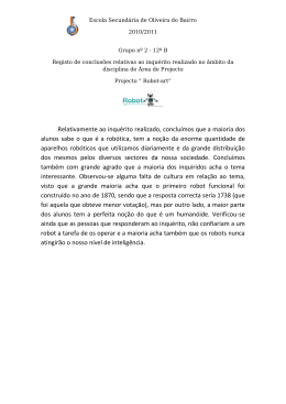
A NEURAL APPROACH TO REAL TIME COLOUR RECOGNITION IN THE
ROBOT SOCCER DOMAIN
José Angelo Gurzoni Jr.∗, Murilo Fernandes Martins†, Flavio Tonidandel∗, Reinaldo A.
C. Bianchi∗
∗
Dept. of Electrical Engineering
Centro Universitário da FEI, Brazil
†
Dept. of Electrical and Electronic Engineering
Imperial College London, UK
Emails: [email protected], [email protected], [email protected],
[email protected]
Abstract— This paper addresses the problem of colour recognition in real time computer vision systems
applied to the robot soccer domain. The developed work presents a novel combination between our current
model-based computer vision system and neural networks to classify colours and identity the robots on an image.
This combination presents an alternative to the considerably high computational cost of the neural network,
which reduces the demanding and time consuming task of calibrating the system before a match. The results
prove that this new approach copes with luminance variations across the playing field and enhances the accuracy
of the overall system.
Keywords—
1
Neural Networks, computer vision, mobile robotics
INTRODUCTION
Since its introduction to the Artificial Intelligence
research field, the Robot Soccer domain has become a widely studied area of research. The
Robot Soccer domain introduces a real, dynamic
and uncertain environment, requiring real time
responses from a team of robots that must, autonomously, work together to defeat an opponent
team of robots. The reason for such popularity
comes from the diversity of challenges addressed
by this domain in many areas of research, including machine learning, multi-robot systems, computer vision, control theory and so forth.
A robot soccer team must be endowed with
sensory and perceptual capabilities in order to actuate in the environment. The richest perceptual
data of a robot soccer system is, for sure, provided
by the computer vision system, responsible for the
recognition of the robots and ball pose. The computer vision system must retrieve the pose of the
objects recognised in the scene accurately, in real
time and should cope with luminance variation,
occlusion, lens distortion and so forth. Notice
that, as different teams and even robots are distinguished by different colours, the computer vision system must recognise these colours in order
to provide the right information about the scene
observed.
Although largely studied by several researchers (e.g., (Comaniciu and Meer, 1997),
(Bruce et al., 2000)), colour segmentation is still
an open issue and worthy of consideration, as recent studies like (Tao et al., 2007), (Sridharan and
Stone, 2007) and (Zickler et al., 2009) have shown.
This is due to difficulties in dealing effectively with
luminance variation and colour calibration.
In our previous work (see (Martins et al.,
2006), (Martins et al., 2007)) we developed a
model-based computer vision system that does not
use colour information for object recognition, only
for object distinction. As a result, this system
proved to be fast to recognise objects and also robust to luminance variation. It also made the task
of calibrating colours easier, since this information
is only required when the objects are already detected in the image. However, the calibration of
colours was still required.
Moving towards an automatic computer vision system, we present in this paper a novel combination between our model-based computer vision system and a Multi-layer perceptron (MLP)
neural network to classify colours as an alternative
to the high computational cost of neural networks,
enhancing the accuracy of the overall system.
We first examine colour and object recognition issues and define the problem in Section 2.
Subsequently, in Section 3 we present a brief review of the relevant characteristics of Artificial
Neural Networks for the problem of colour classification and, in Section 4, describe our approach
to solve the problem stated. Section 5 has descriptions and analysis of the experiments performed,
followed by the paper conclusion, Section 6, where
we remark the contributions and present future
work.
2 COLOUR AND OBJECT
RECOGNITION IN ROBOT SOCCER
The robot soccer domain is composed of a group of
distinct categories, which are regulated by either
FIRA or RoboCup. These categories range from
small-sized wheeled mobile and dog-like 4-legged
robots to humanoid robots, offering to researchers
Figure 1: The MiroSot arquitecture proposed by
FIRA
two main challenges in computer vision: local and
global vision systems.
The former requires robots endowed with such
an embedded system (camera and computer vision
algorithms) that allows the robot to localise the
ball, the other robots (teammates and opponents)
and itself. The latter entails a system where the
camera is fixed over the game field, providing a
global perception of the environment and centralising the processing of the images captured by the
camera, as illustrated in Fig. 1.
2.1
The RoboFEI global vision system
We have been developing a global vision system
for the RoboFEI robot soccer team, under the
rules of the MiroSot, regulated by FIRA. Basically, each team is represented by a colour, either
yellow or blue, and the ball is an orange coloured
golf ball. A label must be placed on top of each
robot with a blob coloured according to the team
the robot represents and a minimum area of 15
cm2 .
To distinguish between robots in our team,
another blob with a different colour (green, cyan
or pink) is placed on the label and we deliberatively use a circle as the shape of the blobs. The
circles are posed in such a way that the line segment between their centres forms an angle of 45
degrees with the front of the robot (Fig. 2).
In order to recognise the objects (robots and
ball), the computer vision system was designed in
seven stages, as shown in Fig. 3 (for a detailed
description, see (Martins et al., 2006), (Martins
et al., 2007)).
Initially, the images are captured from the
camera with resolution of either 320x240 or
640x480 pixels and 24-bit RGB colour depth, at
30 frames per second. Then, the background is
subtracted so only the objects remain in the im-
Figure 2: Example of a label used to identify the
robots
Figure 3: Block diagram of the RoboFEI global
vision system
age, and the edges are extracted.
Subsequently, the Hough Transform, fitted to
detect circles, is computed using only edge information and hence a Hough space is generated,
which maps cartesian coordinates into probabilities. The higher the probability the higher the
certainty that a given point is centre of a real circle in the image. The Hough space is thresholded
and the points with the highest probabilities are
stored to be used afterwards.
Finally, the robots are recognised using colour
information, since all the circle centres in the image are already known (the high probability points
in the Hough space). By using this approach, the
influence of luminance variation is considerably
minimised and the accuracy required to calibrate
the colours is reduced.
However, the colour recognition in the Object
Recognition stage is based on a set of constant
thresholds (minimum and maximum values for
Hue, Saturation and Value) for each colour class.
The use of constant thresholds implies in two main
limitations: (i) the minimum and maximum HSV
values can only be set as continuous ranges, while
the number of discontinuities is not known, and
(ii) the ranges of HSV must be adjusted for each
colour in such a way that these ranges are neither so narrow that cannot represent all possible
samples of a class, nor too wide that two colour
ranges get superposed. Due to these restrictions,
the task of calibrating colours is demanding and
time consuming, requiring knowledge of theoretical concepts, such as the HSV colour space representation and how each attribute of this colour
space influences colour information.
Many researchers have been addressing the
colour calibration procedure (e.g., (Gunnarsson
et al., 2005), (Sridharan and Stone, 2007)) in
different categories, proposing new techniques to
solve the problems of manual colour calibration
systems. Our approach in this paper (described
further in Section 4) makes use of Artificial Neural Networks.
3
NEURAL NETWORKS TO
RECOGNISE COLOURS
Artificial Neural Networks, particularly Multi
Layer Perceptron (MLP) networks, have been applied to a wide range of problems such as pattern
recognition and robot control strategies, noticeably for their capability of approximating nonlinear functions, by learning from input-output
example pairs, and generalisation (see (Mitchell,
1997)). MLP neural networks can learn from complex and noisy training sets without the need to
explicitly define the function to be approximated,
which is usually multi-variable, non-linear or unknown. In addition, they also have the capability
to generalise, retrieving correct outputs when input data not used in the training set is presented.
This generalisation allows the use of a small number of samples during the training stage.
Specifically in the problem of colour classification, the representation of the colour classes
in the HSV domain (as stated in Section 2.1)
can be spread along a variable, and unknown a
priori, number of discontinuous portions of the
space, which a manually-defined thresholding system cannot represent unless it has one set of
thresholds for each of these discontinuous portions. The creation of multiple thresholds also
considerably increase the expertise and time required to calibrate the colours, if the task is to be
carried manually by the operator. On the other
hand, this representation can be quickly learnt by
neural networks from the training set, without the
need of operator’s expertise, making them a much
more suitable solution for the task.
However, MLP neural networks have a relatively high computational cost, due to the fact
that each new input sample requires a new calculation of the neuron matrices, which cannot be
computed a priori, thus making MLPs to be commonly deemed unsuitable for real time applications. Next section details a way to overcome this
inconvenience and have neural networks applied
to a real time application.
Figure 4: The MLP neural network implemented
to recognise colours
4
THE IMPLEMENTED SYSTEM
In order to be fully compatible with the modelbased vision system used in this paper, the MLP
neural network algorithm was implemented in
C/C++ language, and the machine learning portion of the well-known Intel OpenCV library due
to its very good performance.
The MLP neural network is composed of 3
layers of neurons, activated by sigmoid functions.
Because the input is a 3 dimensional vector, the
HSV colour space, 3 neurons form the input layer,
while the output layer has 7 neurons, six outputs
representing a given colour of interest in which
a pixel must be classified (orange, yellow, blue,
green, pink and cyan) and an additional output
representing the background. Regarding the hidden layer, after some preliminary investigations we
found the best accuracy using 20 neurons. Therefore, the topology of the MLP neural network was
set as 3-20-7. To train the network, the backpropagation with momentum algorithm was used, and
the parameters adjusted to learning rate of 0.1,
momentum of 0.1 and stop criteria (also called
performance) of 10−6 . This tight value for serves to really ensure the training set was learnt
correctly and the scalar value was defined during
the test phase, looking at different values of that
could still produce high fidelity results.
Moving towards an automatic global vision
system, we developed a solution to the colour calibration problem, inspired by the work developed
by (Simoes and Costa, 2000). In order to bypass
the high computational cost constraint, we make
use of our model-based vision system to detect,
through a Hough transform, the points with high
probability of being the actual centres of circles
that form the real objects in the image. Once the
circles are found, we apply the MLP neural network (shown in Fig. 4) to classify the pixels of a
5x5 mask inside this area.
In contrast to our previous method to calibrate colours described in Section 2.1, the task of
training the MLP neural network is straightforward to anyone who is able to distinguish colours,
since no specific knowledge is needed and the only
requirement is to select samples of a given colour
of interest and define to which output that samples should be assigned.
This yields a more efficient use of the MLP
neural network evaluation function, since only
a small number of pixels need to be evaluated,
rather than evaluating the whole image. For instance, in an image with resolution of 320x240
pixels (the lowest resolution we use), the neural network would need to classify 76800 points,
while with the combination of our model-based
system the number of points to be classified is reduced to 1250 (about 50 points with probability
higher than a fixed threshold - for more details,
see (Martins et al., 2006), (Martins et al., 2007)),
because only a 5x5 pixel mask of each detected
circle needs to be evaluated. This reduction, as
shown by the results further presented, is enough
to allow the execution of the network in real time.
5
EXPERIMENTS
In order to validate our proposal and analyse the
performance of the MLP neural network implemented, we performed experiments to measure accuracy and execution time of the algorithm, as
well as a complete real-world scenario test. Below we describe the MLP neural network training
stage and the three experiments performed.
In the first experiment, the MLP neural network was tested detached from the model-based
vision system, aiming at measuring its accuracy.
Subsequently, the second experiment tested our
combined solution to object recognition, focusing
on the accuracy and execution time of the complete vision system when compared with the manual calibration of the colour ranges. The third test
is a real-world test, with measurements of accuracy taken directly from a game scenario.
In all cases, the tests were performed on
a computer equipped with an Intel Pentium D
3.4GHz processor running Microsoft Windows XP
operating system.
5.1
The MLP neural network training stage
In our approach, the training stage happens before a game, when a human supervisor selects
the training points in the image and defines to
which output (either a colour or background)
these points should be classified. In this scenario,
we take advantage of capturing the input samples
in a live video streaming, what takes into account
the noise. As points are captured from different
frames, they intrinsically carry the noise to the
training set, improving the robustness of the neural network. Once enough training points are captured, the human triggers the network’s training
function.
5.2
Neural Network accuracy test
In this test, we trained the neural network using
140 training points, 70 from an image with luminance of 750 lux and other 70 from another image
with luminance of 400 lux, with the training points
equally distributed among the 7 output classes.
The network was then executed against 10x76800
pixels (10 images with resolution of 320x240 pixels and luminance varying from 400 to 1000 lux).
The result was an average of 83% correctly classified pixels. The source image and resultant representation of the classified pixels are shown in
Fig. 5. From the image is noticeable that most
of the incorrectly classified pixels belong to the
Figure 5: (top) Source image from noisy camera.
(bottom) Resultant image, generated by the Neural network classification
background class, what does not pose a problem
for the algorithm, since the colour information is
only retrieved from points belonging to the foreground image, after background subtraction. This
experiment proves that our MLP neural network
is robust to luminance variation and the accuracy
is high enough to be used on our approach in
the robot soccer domain. However, this test is
a proof of concept, aimed at validating the algorithm. The practical application of the proposed algorithm is presented in the following experiments.
5.3
Manual thresholding x Neural approaches
comparison
In this test, we used 30 images of the game field
with the objects (6 robots and a ball) randomly
positioned on the field, captured at the resolution
of 640x480 pixels.
Three people (first two with basic knowledge
and one with advanced skills in regards to our
computer vision system) were asked to calibrate
the manual colour recognition system. In addition, each one was asked to capture 140 training
points (20 for each output class) to train the MLP
neural network, always using the same image. A
fourth person then presented the 30 images to the
computer vision system and obtained the results
shown in Table 1 for both algorithms. During this
experiment, the averaged execution times of the
complete vision system were also measured, within
a loop of 500 executions for each test image, and
the results are shown in Table 2.
While both algorithms produced good classification levels, the neural network showed not to
be easily susceptible to performance drops caused
by different trainer experiences, expressed by its
much smaller deviation on the experiments, and
to match and exceed the thresholding algorithm
performance. In terms of execution time, we conclude that no significant time is added with the
introduction of the neural network algorithm.
Table 1: Accuracy (%)
Thresholding Neural Network
1st trainer
90 ± 14.2
97.5 ± 2.3
2nd trainer
76 ± 29.0
97.5 ± 3.5
3rd trainer
96 ± 21.0
96 ± 2.3
Figure 6: Percentage of frames where the robots
were found, averaged among 6 robots of different
colour combinations, by each algorithm.
Table 2: Execution times (ms)
Image Size
Algorithm
320x240
640x480
Neural Network 7.92 ± 1.15 27.30 ± 1.76
Thresholding
6.10 ± 0.01 25.55 ± 0.28
5.4
Real Game Scenario
At last, we tested and compared the algorithm
in a real game scenario, with luminance variations and using real time images from the camera.
This is a very similar complete system validation
test we performed in our previous work (Martins
et al., 2007), with the difference that, this time,
we used a camera with noisy signal. The noisy
colour signal is a very common noise found specially in analog cameras, caused by imperfect or
old cabling connections, electric wiring close to
video signal cables and aging cameras. Under luminance variation and noise conditions, we sought
to stress the capabilities of the neural algorithm to
generalise, correctly classifying pixels of different
luminance levels, even when trained and executed
with noisy samples.
To do so, the neural algorithm was calibrated
with 70 samples from the live camera image, 35
of these obtained at a luminance level of 1000 lux
and 35 obtained at 600 lux. As the thresholding
algorithm would need to be used as comparison,
it was calibrated as well, with some static images
taken at different luminance levels, as the paragraph of result analysis will explain. Then, the
robots were set to randomly run across the field
and a counter summed the number of times each
robot was correctly identified, in a cycle of 4000
frames, in a process that was repeated for each
Figure 7: Percentage of frames where the robot
with smaller detection count was found by each
algorithm.
different luminance level. Fig. 6 shows the averaged detection count among the 6 robots, comparing the neural and threshold algorithms. Fig.
7 shows a worst case detection count, of the robot
detected the lesser number of times during one
cycle of 4000 frames. The game test results show
that the neural algorithm is extremely robust to
luminance variation, as well as to noise. On the
contrary, the thresholding system is highly vulnerable to noise. It is important to note also that,
to obtain a calibration for the thresholding algorithm that could be used in the test, more than
45 minutes where spent in trials, for even when
the results in the test images were satisfactory,
after the robots started to move the results were
showed to be poor. The neural network calibration did not take more than 3 minutes and was
executed only one time.
6
CONCLUSIONS AND FUTURE
WORK
The results of the different experiments confirm
that our approach, combining object detection
and neural network colour classification, considerably increases the accuracy of the vision system
under real-world conditions such as noise and light
intensity variation while, at same time, creates
an easier to operate method for colour recognition. We successfully removed the time consuming and demanding task of manually adjusting
thresholds for colour calibration and replaced it
by a more robust and efficient classifier, the neural network, but avoided its high computational
cost with the use of the circle detection algorithm
based in Canny and Hough filters. The limitation of the system is its inability to detect objects
with unknown geometric form, which we intend
to solve in future work. We would like also, as a
future work, to explore the use of non supervised
classifiers and possibly RBF (Radial Basis Function) neural networks, aiming to produce a fully
automatic calibration system.
ACKNOWLEDGMENTS
The authors would like to thank FAPESP, CNPq
and CAPES for the support.
Murilo Fernandes Martins acknowledges the support of
CAPES (Grant No. 5031/06-0) and Reinaldo A.
C. Bianchi acknowledges the support of CNPq
(Grant No. 201591/2007-3) and FAPESP (Grant
No. 2009/11256-0).
The authors are also very grateful to the members of the RoboFEI project, for their valuable
contributions and time spared.
References
Bruce, J., Balch, T. and Veloso, M. (2000). Fast
and inexpensive color image segmentation
for interactive robots, Proceedings of IROS2000, Japan.
Comaniciu, D. and Meer, P. (1997). Robust analysis of feature spaces: color image segmentation, CVPR ’97: Proceedings of the 1997
Conference on Computer Vision and Pattern
Recognition (CVPR ’97), IEEE Computer
Society, Washington, DC, USA.
Gunnarsson, K., Wiesel, F. and Rojas, R. (2005).
The color and the shape: Automatic online color calibration for autonomous robots,
in A. Bredenfeld, A. Jacoff, I. Noda and
Y. Takahashi (eds), RoboCup, Vol. 4020 of
Lecture Notes in Computer Science, Springer,
pp. 347–358.
Martins, M. F., Tonidandel, F. and Bianchi, R.
A. C. (2006). A fast model-based vision system for a robot soccer team, in A. F. Gelbukh and C. A. R. Garcı́a (eds), MICAI, Vol.
4293 of Lecture Notes in Computer Science,
Springer, pp. 704–714.
Martins, M. F., Tonidandel, F. and Bianchi, R.
A. C. (2007). Towards model-based vision
systems for robot soccer teams, in P. Lima
(ed.), Robotic Soccer, I-Tech Education and
Publishing, chapter 5, pp. 95–108.
Mitchell, T. (1997). Machine Learning, McGrawHill Education (ISE Editions).
Simoes, A. S. and Costa, A. H. R. (2000). Using
neural color classification in robotic soccer
domain, International Joint Conference IBERAMIA’00 Ibero-American Conference on
Artificial Intelligence and SBIA’00 Brazilian
Symposium on Artificial Intelligence pp. 208–
213.
Sridharan, M. and Stone, P. (2007). Color learning
on a mobile robot: Towards full autonomy
under changing illumination, in M. M. Veloso
(ed.), IJCAI, pp. 2212–2217.
Tao, W., Jin, H. and Zhang, Y. (2007). Color image segmentation based on mean shift and
normalized cuts, Systems, Man, and Cybernetics, Part B, IEEE Transactions on
37(5): 1382–1389.
Zickler, S., Laue, T., Birbach, O., Wongphati,
M. and Veloso, M. (2009). Ssl-vision: The
shared vision system for the robocup smallsize league, Proceedings of the International
RoboCup Symposium 2009 (RoboCup 2009).
ABORDAGEM GENÉTICA PARA DEFINIÇÃO DE AÇÕES EM AMBIENTE
SIMULADO DE FUTEBOL DE ROBÔS
Eduardo Sacogne Fraccaroli∗, Ivan Nunes da Silva∗
∗
Av. Trabalhador Sancarlense, 400, 13566-590, São Carlos
Universidade de São Paulo, Escola de Engenharia de São Carlos, Departamento de Engenharia Elétrica
São Carlos, São Paulo, Brasil
Emails: [email protected], [email protected]
Abstract— This work consists of applying a genetic algorithm as an alternative approach to traditional methods for defining the actions of the players on a soccer team of robots simulated. The method of evaluation of
each team is based on the number of goals for and goals against. It is a robust method of evaluation, which is
focused on the distinction of global acions according to the types of players (defender, attacker and middle field).
The results are reported in order to validate the presented proposal.
Keywords—
Genetic Algorithm, Multi-Agent System, RoboCup 2D.
Resumo— Este trabalho consiste na aplicação de um algoritmo genético como alternativa aos métodos tradicionais para definir as ações dos jogadores em um time de futebol de robôs simulados. O método de avaliação de
cada time é baseada no número de gols prós e gols contra. Propõe-se um método de avaliação robusto, focado
na distinção das ações globais conforme os tipos de jogadores (zagueiro, meio campo e atacante). Os resultados
são relatados procurando validar a proposta apresentada.
Palavras-chave—
1
Algoritmos Genéticos, Sistemas Multi-Agentes, RoboCup 2D.
Introdução
As pesquisas em sistemas multiagentes têm se tornado uma das principais tendências no domı́nio da
inteligência artificial (Weiss, 1999). O conceito de
futebol de robôs foi introduzido em 1993 pelo Dr.
Itsuki Nota (Kitano et al., 1995). A competição
de futebol de robôs tem como pretexto o desenvolvimento de técnicas de inteligência artificial, para
aplicações robóticas, utilizando um problema padrão em que um grande leque de possı́veis tecnologias possam ser examinadas. Aprendizado por
reforço, aprendizado por reforço baseado em heurı́sticas, algoritmos genéticos, sistemas fuzzy e redes neurais artificiais são as tecnologias mais utilizadas no ambiente de futebol de robôs.
A partir de já há muito tempo, um dos objetivos mais perseguidos pelo ser humano é dotar uma máquina construı́da pelo mesmo com
caracterı́sticas inteligentes. Desde então, têmse testemunhado o surgimento de novos paradigmas simbólicos de aprendizagem, em que muitos
deles se tornaram métodos computacionais poderosos, como aprendizado baseado em explicações, sistemas classificadores e sistemas evolutivos
(Ross, 2004).
O algoritmo genético é inspirado na teoria da
evolução de Darwin e pode ser considerado como
um método que trabalha com buscas paralelas
randômicas direcionadas, em que se utiliza o processo evolutivo para determinar a melhor (mais
adequada) solução de um problema. São empregados para resolver problemas complexos, tendo
como vantagem seu paralelismo. O algoritmo genético percorre o espaço das possı́veis soluções
usando muito indivı́duos, de modo que são me-
nos susceptı́veis de ficarem presos em um mı́nimo
local (Goldberg, 1989).
Existem diversas pesquisas realizadas na área
da RoboCup nas quais se utilizam algoritmos genéticos. Em Nakashima et al. (2004) foi proposto
um método evolutivo para aquisição da estratégia
do time, em que se utilizou um conjunto de regras
para inferir uma determinada ação de acordo com
a posição do jogador e do adversário mais próximo. Já em Nakashima et al. (2006) foi proposto
um método utilizando correspondência histórica.
A avaliação de um time é realizada de acordo com
seus objetivos e suas metas, portanto, é possı́vel
que um time com uma boa estratégia seja eliminado, devido isto ao fato do ambiente simulado
possuir um alto grau de incerteza.
Assim sendo, para os propósitos mencionados
anteriormente, o restante deste artigo está organizado da maneira que se segue. A Seção 2 apresenta uma breve descrição sobre a RoboCup. A
Seção 3 descreve o ambiente de simulação de futebol de robôs e seus respectivos módulos. A Seção
4 introduz o conceito do algoritmo genético e seus
principais operadores. A Seção 5 apresenta o modelo do time e suas respectivas ações propostas. A
Seção 6 detalha o modelo proposto do algoritmo
genético. A Seção 7 mostra os resultados obtidos
de acordo com o número de gerações. Finalmente,
as conclusões são tecidas na Seção 8.
2
Aspectos da RoboCup
A RoboCup (Robot World Cup) foi iniciada no Japão e nos Estados Unidos e tem como ambicioso
objetivo criar um time de robôs humanóides, to-
talmente autônomos, capazes de ganhar dos atuais
campeões mundiais de futebol. A RoboCup possibilita pesquisas nas áreas de robótica e inteligência
artificial, disponibilizando um problema desafiador que oferece a integração de pesquisas nas diversas áreas da robótica e da inteligência artificial,
por exemplo, agentes autônomos, visão computacional, colaboração multiagente, comportamento
reativo, aprendizado, controle de movimento, controle inteligente robótico, evolução, resolução em
tempo real, entre outros (Kitano et al., 1998).
Existem cinco categorias na RoboCup Soccer : Humanoid, Middle Size, Small Size, Standard
Platform e Simulation. Cada uma com o foco em
diferentes nı́veis de abstração para o respectivo
problema.
3
Categoria de Simulação 2D
O ambiente dos agentes simulados é uma estrutura
hierárquica. Essa estrutura é dividida em dois ambientes. O ambiente de baixo nı́vel é responsável
por processar as informações básicas como aquelas
de informações visuais, de som, de sensibilidade e,
também, de ações básicas como driblar, realizar
um passe e chutar. O outro é o ambiente de alto
nı́vel que possibilita a decisão do ponto de vista
global, tais como a estratégia cooperativa de jogar
entre os companheiros (Chen et al., 2002).
O ambiente da RoboCup Simulação 2D apresenta as caracterı́sticas de ser um ambiente dinâmico em tempo real, ruidoso (insere um ruı́do
gaussiano entre a comunicação servidor/cliente),
cooperativo e coordenado e de possuir limitado
espaço de comunicação.
uso de ferramentas que viabilizem a comunicação
via UDP/IP, pois toda comunicação feita entre o
servidor e cada cliente é feita via socket UDP/IP,
o qual é um protocolo de comunicação orientado
à conexão, incluindo-se mecanismos para iniciar
e encerrar a conexão, negociar tamanhos de pacotes e permitir a retransmissão de pacotes corrompidos. Cada cliente é um processo separado e
conecta-se com o servidor por meio de uma única
porta. Cada time pode ter onze clientes (jogadores).
O cliente é responsável por atuar no ambiente simulado, sendo este o módulo em que são
desenvolvidos e aplicados os algoritmos inteligentes para serem avaliados. As ações referentes ao
comportamento dos jogadores devem ser executadas obedecendo a ordem seguinte . Primeiro, o
cliente envia requisições para o servidor; em seguida, o servidor recebe e armazena as requisições, as quais são procuradas para serem executadas (chutar a bola, virar, correr, etc.); por fim,
o ambiente é então atualizado. O servidor é um
sistema executado em tempo real com intervalos
discretos de tempo (ciclos) (Chen et al., 2002).
Figura 2: Simulação computacinal de uma partida de
futebol de robôs simulados.
Figura 1: Arquitetura do simulador 2D.
(Reis, 2003).
O ambiente simulado de futebol de robôs é
composto por dois módulos, ou seja, o servidor e
o monitor. O servidor é um ambiente que torna
possı́vel o jogo de futebol entre dois times, sendo
responsável por simular os movimentos dos jogadores e da bola, a comunicação com cliente (jogador) e o controle do jogo conforme as regras. Para
desenvolver times torna-se necessário que se faça
O monitor (Figura 2) é responsável por mostrar o campo na tela do computador. Por meio
dessa interface é possı́vel observar os agentes jogando de acordo com as informações enviadas pelo
servidor. As informações disponı́veis na tela incluem o placar, os nomes dos times, o tempo decorrido, os jogadores, as posições e a bola (Chen
et al., 2002).
4
Algoritmo Genético
Os algoritmos genéticos foram introduzidos por
Holland (1975), com o objetivo de simular por
meio de um computador os processos de adaptação de sistemas naturais utilizando um sistema
artificial.
Pseudocódigo Algoritmo Genético
begin
Geração ←− 0;
Inicializar População (Geração);
Avaliar População (Geração);
while (Não Condição de Parada) do
Geração ←− Geração + 1;
Selecionar População (Geração)
a partir da População (Geração - 1);
Alterar População (Geração);
Avaliar População (Geração);
end while
end
Figura 3: Pseudocódigo do algoritmo genético.
Os algoritmos genéticos são técnicas de busca
estocásticas inspiradas na teoria de Darwin, que
consiste em achar uma resposta para um problema com um número grande de possı́veis soluções. Charles Darwin propôs a teoria da seleção
natural, na qual indivı́duos com boas caracterı́sticas genéticas possuem maiores chances de sobrevivência e de se reproduzirem, gerando-se, assim,
indivı́duos cada vez mais aptos. Por outro lado,
os indivı́duos menos aptos tenderão a desaparecer (Holland, 1975). Na Figura 3 é mostrado um
pseudocódigo resumido de um algoritmo genético.
Um algoritmo genético deve apresentar os seguintes componentes:
• Um método de seleção genética para soluções
candidatas ou potenciais;
• Uma maneira de gerar uma população inicial
para as possı́veis soluções potenciais;
• Uma função para avaliar sua adaptação ao
ambiente;
• Operadores genéticos, como cruzamento e
mutação.
Uma população inicial de cromossomos pode
ser criada usando uma seleção aleatória de cada
gene. Cada um dos cromossomos deve ser avaliado de acordo com seu sucesso em direção à solução do problema, sendo que tal avaliação é obtida por meio da função objetivo (fitness), cuja
missão é estabelecer uma relação que permita medir o desempenho de cada solução. Os indivı́duos
com melhores desempenhos serão escolhidos para
se reproduzirem. Já os indivı́duos menos aptos serão retirados da população e substituı́dos por seus
descendentes. Cada iteração em um algoritmo genético é conhecida como geração.
Os algoritmos genéticos possuem um operador
de seleção, o qual é responsável por selecionar o
cromossomo com melhor valor de avaliação. Para
reproduzir dois descendentes, os cromossomos são
trocados em um ponto determinado.
Em cada geração uma mutação em um gene
especı́fico pode ocorrer, sendo a mesma essencial
por dois motivos. Primeiro, na natureza, mutações podem ocorrer de maneira aleatória. Segundo e mais importante, em um contexto de um
problema otimista, isso impede que a população
se torne uniforme e incapaz de se desenvolver e,
também, prevê a possibilidade de saltar pontos
de mı́nimos locais. A probabilidade da mutação
pode ser representada por meio de um operador
de mutação, em que cada gene em um cromossomo tem a mesma probabilidade de ser mutado
(Rezende, 2003).
5
Caracterı́sticas do Time
Nesse artigo utiliza-se o time UvA Trilearn como
base para aplicar o modelo evolutivo computacional. O código fonte apenas implementa o comportamento de baixo nı́vel, como informações trocadas com o servidor. O comportamento de alto
nı́vel, como a estratégia do time foi omitida no
código fonte.
Assim, encontra-se disponı́vel somente dois
modos simples de ações no código da UvA Trilearn. Um é o modo de manuseio da bola e o outro
é o modo de posicionamento, os quais serão utilizados pelos jogadores dependendo da situação de
jogo. Se o jogador estiver perto da bola, o modo
manuseio da bola é então executado. Este modo
é executado quando o jogador está perto da bola,
o qual avalia a possibilidade de chutar ou não;
se existir a possibilidade de chutar, o mesmo realizará uma ação consequente; por outro lado, se
não existir tal possibilidade, haverá então a ação
de interceptar a bola. A ação de interceptar a
bola consiste em posicionar o jogador no ponto
de intersecção da trajetória da bola (de Boer and
Kok, 2002).
Foram propostas 10 ações nesse artigo, tais
quais:
1. Realizar um passe com velocidade média para
o companheiro número seis;
2. Realizar um passe com velocidade média para
o companheiro número sete;
3. Realizar um passe com velocidade média para
o companheiro número oito;
4. Levar a bola para uma área sem oponentes,
usado quando não conseguir driblar ou realizar o passe para o companheiro;
5. Chutar em direção ao gol adversário;
6. Driblar em direção à linha lateral com um
ângulo positivo;
7. Driblar em direção à linha lateral com um
ângulo negativo;
8. Realizar um passe com velocidade alta para
o companheiro número nove;
9. Realizar um passe com velocidade alta para
o companheiro número dez;
10. Realizar um passe com velocidade alta para
o companheiro número onze.
A Figura 4 representa os indivı́duos (jogadores) gerados e suas respectivas ações. Cada indivı́duo (jogador) possui um conjunto de ações de
1 a 10. Gera-se de 1 a 10 indivı́duos para cada
geração.
de uma partida comum de futebol no ambiente simulado costuma ser de dez minutos, dividido em
dois tempos de cinco minutos cada. A cada geração são criados dez indivı́duos (jogadores), sendo
necessário dez minutos para avaliar o time. Para
acelerar o processo de avaliação foi necessário configurar o servidor, alterando-se a variável que controla o sincronismo. Foi alterado do modo sı́ncrono para o modo não sı́ncrono, acelerando-se
assim o tempo de uma partida. Desse modo, o
tempo decorrido passa a ser aproximadamente de
dois minutos e meio, reduzindo-se então o processo
de avaliação de cada geração.
Figura 4: Representação dos jogadores.
Os quatro primeiros jogadores exercerão a
função de zagueiros, os três jogadores intermediários exercerão a função de meio-campo e os últimos três jogadores exercerão a função de atacantes.
6
Desenvolvimento do Sistema
Propõe-se aqui um método evolucionário para obter a estratégia para os jogadores e que seja eficiente para o propósito de se jogar futebol. O foco é
tentar encontrar o melhor conjunto de ações para
os dez jogadores. Cada jogador possui seu próprio conjunto de ações que serão utilizados quando
estiver de posse da bola. Toda estratégia está armazenada dentro de um vetor de números inteiros.
Ressalta-se que o foco não é otimizar um jogador
unicamente e sim o time como um todo.
O algoritmo genético foi aplicado somente
nos dez jogadores, sendo que o goleiro foi excluı́do. Considerando o total de ações por jogador, utilizaram-se então os dez vetores de inteiros
para representar o time. Cada vetor possui dez
possı́veis ações de um jogador e cada posição do
vetor pode assumir valores no intervalo de [1,10],
de acordo com as dez possı́veis ações descrita na
Seção 5. Cada ação é realizada na sequência correspondente ao do vetor de inteiros, no momento
em que o jogador estiver de posse da bola .
No processo de avaliação, cada vetor de inteiros na população joga apenas uma vez. A avaliação é baseada no resultado do jogo, realizado contra o time base UvA Trilearn. O tempo decorrido
Figura 5: Fluxograma do algoritmo genético.
A Figura 5 apresenta o fluxograma do algoritmo genético proposto. Primeiramente, é gerado
apenas um time de dez indivı́duos aleatoriamente.
Então, esse time gerado é colocado para disputar
uma partida de futebol. Após o término da partida, o referido time é avaliado de acordo com o
placar resultante. Dependendo do resultado cada
indivı́duo, ao ser avaliado, obterá um valor diferente de fitness, correspondente a sua respectiva
função de atuação em campo.
O método de avaliação prioriza o valor de gols
prós em relação ao valor de gols contra. Quando
a partida é finalizada, dois valores são retornados
para a função de avaliação, isto é, a quantidade de
gols prós e a quantidade de gols contra. O função
de avaliação recebe o placar da partida e pontua
cada indivı́duo de acordo com sua posição tática.
Em seguida, realiza-se o cruzamento e a mutação
dos indivı́duos selecionados de acordo com suas
respectivas pontuações.
O algoritmo genético foi configurado com as
seguintes caracterı́sticas:
• Processo de avaliação utilizando recompensa
e punição;
• Cruzamento usando apenas um ponto em
60% dos indivı́duos;
• Mutação em apenas 1% dos indivı́duos;
• Método de seleção do tipo elitista.
Na operação de cruzamento é selecionado
60% da população pelo método do elitismo,
respeitando-se os indivı́duos com melhores valores da função de avaliação. Tal método elenca
os indivı́duos de acordo com o valor da função de
avaliação, do maior valor para o menor valor desta
função, mantendo-se os indivı́duos mais aptos na
população.
Depois de se selecionar 60% do indivı́duos,
escolhe-se aleatoriamente um ponto de secção para
realizar a operação de cruzamento, em que serão
trocados as duas metades dos dois vetores selecionados anteriormente. Dois indivı́duos (pais) geram, a partir do método de cruzamento, dois novos indivı́duos (filhos).
Para a operação de mutação, um indivı́duo é
escolhido aleatoriamente. Em seguida, escolhe-se
um ponto dentro do seu vetor de inteiros para realizar a mutação, obedecendo-se os seguintes critérios:
• Se o indivı́duo for um zagueiro, priorizar então as ações 1, 2, 3, 4, 5, 6 e 7;
• Se o indivı́duo for do tipo meio campo, priorizar então as ações 4, 5, 6, 7, 8, 9 e 10;
• Se o indivı́duo for um atacante, priorizar então as ações 4, 5, 6 e 7.
O sistema desenvolvido funciona de acordo
com a Figura 6. Primeiramente, geram-se de
maneira aleatória dez indivı́duos (jogadores), os
quais são escritos dentro de um arquivo texto (indiv.txt). O módulo Time lê os indivı́duos desse
arquivo e os colocam para disputar uma partida
no simulador de futebol.
Logo após o término da partida, o simulador
retorna o placar do jogo, sendo que o mesmo é
escrito pelo módulo Time no arquivo texto (placar.txt). Em seguida, o módulo Algoritmo Genético lê o placar desse arquivo e inicia os operadores
genéticos que irão avaliar, cruzar e mutar os indivı́duos. Depois, os indivı́duos são escritos dentro
do arquivo texto (indiv.txt), em que o processo se
reinicia até que o número de gerações seja igual
ao valor definido.
7
Figura 6: Fluxo de dados dentro do sistema desenvolvido.
de 2000 gerações, visando-se avaliar o desempenho do algoritmo genético. A partir da Tabela 1 é
possı́vel notar a evolução do time em relação aos
gols prós e gols contra de acordo com as gerações.
O número de gols prós aumenta conforme o número de gerações e o número de gols contra tende
a cair. Os valores de gols prós e gols contra se
estabilizam após a duo-milésima geração.
Tabela 1: Média de gols prós e gols.
Gerações
Gols Pró
Gols Contra
50
1,2
2,3
100
1,9
1,8
500
2,9
2,6
1000
3,4
2,2
2000
4,1
2,8
A Figura 7 mostra a média de gols prós e gols
contra em relação a cada geração. Foi analisado o
desempenho dos dez indivı́duos (jogadores) como
um todo, após terem sido selecionados como a próxima geração. Percebe-se que houve um incremento do desempenho de acordo com o aumento
do número de gerações, fato este ocasionado pelo
objetivo traçado, no qual consiste em priorizar o
maior número de gols prós.
Resultados de Simulação
Os parâmetros do algoritmo genético foram ajustados conforme a Seção 6. Foram gerados dez indivı́duos (jogadores) de modo aleatório e colocados
para disputar uma partida. Estipulou-se um total
Figura 7: Resultado da simulação.
Nota-se ainda pela Figura 7 aquele resultado
já esperado, ou seja, o aumento da quantidade de
gols prós em detrimento da quantidade de gols
contra. O algoritmo genético foi ajustado de maneira a priorizar determinadas ações em relação à
cada tipo de indivı́duo (jogador), como visto na
Seção 6.
8
Conclusão
Apresentou-se nesse trabalho um modelo capaz de
definir as ações para os respectivos jogadores de
uma partida de futebol de robôs, levando-se em
consideração a função tática em jogo. Para tanto,
utilizou-se um algoritmo genético para determinar
e avaliar o time como um todo em relação aos gols
prós e os gols contra. Em suma, este trabalho possui extrema valia no que tange à especificação de
uma nova estratégia de jogo para times de futebol
de robôs, possibilitando ainda que versões futuras
sejam aprimoradas a partir de novas pesquisas.
Agradecimentos
Os autores gostariam de agradecer à FAPESP
(Fundação de Amparo à Pesquisa do Estado de
São Paulo) e à CAPES (Coordenação de Aperfeiçoamento de Pessoal de Nı́vel Superior) pelos
auxı́lios financeiros propiciados.
Referências
Chen, M., Foroughi, E., Heintz, F., Huang,
Z., Kapetanakis, S., Kostiadis, K., Kummeneje, J., Noda, I., Obst, O., Riley, P.,
Steffens, T., Wang, Y. and Yin, X. (2002).
RoboCup Soccer Server.
Disponı́vel em
http://sourceforge.net/projects/sserver.
de Boer, R. and Kok, J. (2002). The incremental
development of a synthetic multi-agent system: The uva trilearn 2001 robotic soccer simulation team, Master’s thesis, University of
Amsterdam.
Goldberg, D. E. (1989). Genetic Algorithms in Search, Optimization, and Machine Learning,
Addison-Wesley.
Holland, J. H. (1975). Adaptation in Natural and
Artificial Systems, 1 edn, The University of
Michigan Press.
Kitano, H., Asada, M., Kuniyoshi, Y., Noda, I.
and Osawa, E. (1995). Robocup: The robot
world cup initiative, IJCAI-95 Workshop on
Entertainment and AI/Alife.
Kitano, H., Asada, M., Kuniyoshi, Y., Noda, I.
and Osawa, E. (1998). Robocup: A challenge problem for ai and robotics, RoboCup97: Robot Soccer World Cup I.
Nakashima, T., Takatani, M., Ishibuchi, H. and
Nii, M. (2006). The effect os using match
history on the evolutionary of robocup soccer
team strategies, Symposium on Computational Intelligence and Games.
Nakashima, T., Takatani, M., Udo, M. and Ishibuchi, H. (2004). An evolutionary apparoach
for strategy learning in robocup soccer, International Conference on Systems, Man and
Cybernetics.
Reis, L. P. (2003). Coordenação em Sistemas
Multi-Agente: Aplicações na Gestão Universitária e Futebol Robótico, PhD thesis, Faculdade de Engenharia da Univeridade do Porto.
Rezende, S. O. (2003). Sistemas Inteligentes: Fundamentos e Aplicações, Manole.
Ross, T. J. (2004). Fuzzy Logic with Engineering
Applications, John Wiley.
Weiss, G. (1999). Multiagent Systems: A Modern Approach to Distributed Artificial Intelligence, The University of Michigan Press.
SISTEMA ESPECIALISTA FUZZY PARA POSICIONAMENTO DOS JOGADORES APLICADO AO
FUTEBOL DE ROBÔS
JOSÉ R. F. NERI, CARLOS H. F. SANTOS
Grupo de Pesquisas em Robótica(GPR), Centro de Engenharias e Ciências Exatas(CECE), Universidade Estadual do Oeste do Paraná(UNIOESTE) – Campus Foz do Iguaçu
AV. Tancredo Neves, 6731 – CEP 85856-970 – Foz do Iguaçu – PR - Brasil
E-mails: [email protected], [email protected]
JOÃO A. FABRO
Departamento de Informática(DAINF), Universidade Tecnológica Federal do Paraná(UTFPR)
Av. Sete de Setembro, 3165 - CEP 80230-901 - Curitiba - PR - Brasil
E-mail: [email protected]
Abstract¾ This paper presents a proposal of a fuzzy expert system that controls the player positioning in a simulated robot soccer game. The proposed system is based on the Mecateam framework, and on the Expert-Coop++ expert system library. The
proposed system modify the Expert-Coop library using the XFuzzy 3.0 to implement the fuzzy rule-based system. The proposed
system is tested against several other simulated teams from the Robocup finals. Fuzzy expert systems that control the players positioning(including the goalkepper) are implemented, and present a better performance than the non-fuzzy expert system.
Keywords¾ Robot Soccer, Fuzzy Expert Systems, Robocup
Resumo¾ Este artigo apresenta uma proposta de utilização de sistemas especialistas fuzzy para o controle do posicionamento
dos jogadores da categoria "simulação" de um time de futebol de robôs da Robocup. É utilizado o framework Mecateam, e a biblioteca Expert-Coop++, que implementa um Sistema Especialista, é alterada com o apoio da Biblioteca XFuzzy 3.0, para dar
suporte à regras fuzzy de comportamento dos jogadores. São implementadas regras fuzzy de posicionamento do goleiro e dos jogadores, e o desempenho é comparado com outros times que participaram da final nacional da Robocup Brasil, obtendo desempenho superior ao sistema especialista clássico.
Palavras-chave¾ Futebol de Robôs, Sistemas Especialistas Fuzzy, Robocup
1
Introdução
Durante a última década do século XX, a Robocup
(Robot Soccer World Cup) foi uma das organizações
científicas que estabeleceram a promoção e desenvolvimento das pesquisas em Inteligência Artificial
aplicada a robôs móveis inteligentes. No sentido de
realizar estes objetivos, esta organização escolheu o
jogo de futebol como sua aplicação principal. Neste
sentido, várias competições mundiais de futebol de
robôs foram promovidas, onde os times participantes
desenvolveram diversas tecnologias, tais como: controle inteligente, processamento de imagens, colaboração multi-agente, raciocínio e mobilidade em tempo real, aquisição e implementação de estratégias de
jogo, etc (Bishop, 1996).
O objetivo deste avanço tecnológico promovido
pela Robocup é desenvolver até 2050 um time de
robôs humanóides totalmente autônomos que consigam ganhar do atual campeão mundial de futebol
humano. A Robocup é subdividida em várias categorias sendo o robocup soccer a mais importante, abordando o problema do futebol de robôs sendo subdividida em ligas: simulação, robôs pequenos, robôs
médios, robôs com 4 patas, robôs humanóides.
A liga de simulação da Robocup soccer é dividida em duas sub-ligas: 2D e 3D. A categoria simulação funciona simulando uma partida de futebol entre
dois times de onze robôs cada. A arquitetura da categoria de simulação consiste de dois programas, o
soccerserver e o soccermonitor disponibilizados gratuitamente pela comunidade de pesquisa Robocup.
O soccerserver (Figura 1) é um sistema que possibilita agentes autônomos disputarem uma partida de
futebol com outro time. Essa partida é processada no
modo cliente/servidor, sendo que o soccerserver fornece um campo virtual e simula todos os movimentos
dentro dele. Cada cliente (agente) controla as ações
de um jogador simulado, e a comunicação entre o
agente e o servidor é via socket UDP/IP por isso pode-se utilizar qualquer linguagem de programação
que tenha suporte a UDP/IP.
Figura 1. Soccer server.
O soccermonitor (Figura 2) é um programa que
visualiza o campo virtual gerado pelo soccerserver
com dimensões de 105X68 m, em uma janela gráfica.
É uma ferramenta que permite às pessoas visualizarem o que está acontecendo com o soccerserver durante o jogo, ele recebe informações do soccerserver
e as apresenta de modo gráfico.
ta seção, apresenta-se o algoritmo de controle dos
jogadores, destacando-se a coordenação dos jogadores em relação à posição da bola, por exemplo. Na
sexta seção são apresentados os testes dos controladores fuzzy e na sétima e última seção, apresentam-se
as conclusões e algumas idéias que podem servir
como direções para pesquisas futuras.
2
Figura 2. Soccer monitor.
Geralmente, um robô de futebol consiste de uma
parte mecânica, composta por duas rodas, dois motores DC, um microcontrolador, um módulo de comunicação e uma fonte de alimentação. Trata-se de um
relevante exemplo de sistema mecatrônico. O comportamento e eficiência deste robô (agente) dependem de sua construção mecânica, algoritmo de controle e desempenho do sistema de visão.
Este trabalho explora a aplicação de um algoritmo que concilia o controle de um único agente e a
interação deste com os demais agentes do time e os
seus adversários.
Num time de futebol de robôs as principais características individuais são que cada jogador deve
identificar objetos pertencentes ao ambiente como a
bola, e os robôs que compõem o seu time e o time
adversário. Cada jogador deve ser capaz de representar o ambiente, escolher objetivos, planejar e executar ações para atingir as metas do time, como marcar
gols ou posicionar-se na defesa.
Dentre as principais características coletivas destacam-se as de realizar passes, interagir com jogadores do mesmo time para estabelecer ações coletivas
(jogadas ensaiadas), e sincronizar as ações objetivando fazer gols e impedir que o time adversário os faça.
Observa-se que a tarefa de controlar vários agentes não é uma missão fácil, pois deve ser feita de
forma cooperativa, coordenada, e de maneira comunicativa com outros agentes. Neste sentido, propõe-se
uma estratégia cooperativa entre diversos agentes.
Esta estratégia utiliza um algoritmo baseado em lógica nebulosa (fuzzy), a qual é capaz de manipular dados que representam a incerteza das informações
manipuladas, aqui denominado de Sistema Especialista Fuzzy.
Este documento está dividido em sete seções. Na
primeira seção, foi introduzido e contextualizado o
problema e a justificativa de aplicação da proposta.
Na segunda seção, comenta-se sobre o ambiente que
os agentes irão interagir aonde será implementada a
estratégia de controle. Na terceira seção, descreve os
principais conceitos sobre sistemas especialistas
fuzzy e lógica fuzzy. Na quarta seção, é apresentado
a estrutura do controlador fuzzy do goleiro. Na quin-
Framework Mecateam
O framework Mecateam utiliza o código do time de
futebol de robôs Uva Trilearn, da Holanda, para as
camadas mais básicas de programação, e a biblioteca
Expert Coop++ para as camadas onde é implementada a inteligência artificial.
O UvA Trilearn (Kok et al., 2003) é um time de
futebol de robôs simulado da Universidade de Amsterdã, a equipe que desenvolveu os algoritmos de
controle deste time disponibilizou seu código fonte
na internet. Entretanto, somente a parte básica dos
algoritmos foi disponibilizada (chutar a bola para o
gol quando estiver de posse da bola, e posicionar-se
de forma adequada no campo quando estiver sem a
posse da bola). O restante dos algoritmos (a parte
inteligente dos jogadores) foi retirado.
O framework Mecateam disponibilizado e desenvolvido pela UFBA é utilizado como base na elaboração deste projeto.
2.1 Expert-Coop++
A Expert-Coop++ é uma biblioteca orientada a objetos destinada a auxiliar o desenvolvimento de sistemas multiagentes sob restrição de tempo real do tipo
melhor esforço (COSTA et al., 2003). Esta biblioteca
foi implementada em C++ oferecendo suporte a Sistemas Baseados em Conhecimento (SBC). A mesma
utiliza uma arquitetura de três camadas, sendo que
cada uma delas representa um nível decisório distinto
(os níveis são Reativo, Instintivo e Cognitivo).
O nível Reativo é o mais baixo na arquitetura,
encarregado pela interação com o ambiente e pela
resposta em tempo real do agente.
O nível Instintivo consiste de um sistema especialista de um único ciclo de inferência que escolhe a
cada mudança de estado do jogo o comportamento
reativo mais adequado para meta local em vigor.
O nível superior da arquitetura do agente é denominado Cognitivo. O principal papel do nível cognitivo é construir um modelo lógico do ambiente a
partir das informações simbólicas provenientes do
Instintivo, escolhendo planos e avaliando a validade
do plano corrente (JUNIOR, 2007).
3
Sistemas Especialistas Fuzzy
Sistemas especialistas são programas de computador
que usam conhecimento obtido a partir de perícia de
especialista e procedimentos de inferências para auxiliar na tomada de decisão de problemas que requerem
especialidade humana para resolvê-los.
O motor de inferência é o principal componente
do sistema especialista. Seu funcionamento consiste
na realização de inferências a partir de uma base de
regras e uma base de fatos (JUNIOR, 2007).
- A base de fatos é responsável por armazenar o
estado do ambiente e é atualizada a partir de informações do ambiente e das regras.
- A base de regras é responsável pelo armazenamento do conhecimento do especialista.
A lógica fuzzy foi criada visando representar conhecimento incerto e impreciso. Esta lógica fornece
uma maneira aproximada de descrever sistemas bastante complexos, mal definidos, ou de difícil análise
matemática.
Um processo denominado “fuzzificação” gera
entradas fuzzy a partir de dados incertos e imprecisos. Estas informações podem ser então utilizadas
pelo motor de inferência fuzzy, para obter os resultados do processamento das regras. O processo inverso
é chamado de defuzzificação que cria valores reais,
também chamados de crisp, para serem aplicados na
máquina sob controle (máquina ou processo que se
deseja controlar).
4
Figura 3. Gráficos de pertinência.
Um controlador baseado em lógica fuzzy, no entanto, não se preocupa com modelos matemáticos
complexos, baseando o seu controle em regras de
decisão do tipo:
Se x é X, então y é Y.
Abaixo nas tabelas I e II estão definidas a base
de regras para os controladores nos eixos X e Y.
Controlador Nebuloso para o goleiro
Na implementação do sistema especialista fuzzy a
seguir foi proposta a idéia de um algoritmo de controle de posicionamento para o goleiro, de tal forma
que o mesmo se posicione de acordo com a posição
da bola. Esse controlador é ativado quando a bola se
encontra numa certa posição que seria próxima ao
gol. O objetivo desse controlador fuzzy é o posicionamento do goleiro em relação à bola, ele deve se
posicionar na melhor posição para poder recepcionar
a mesma, com o objetivo de fechar o gol e deixar o
atacante com um ângulo ruim para chutar para o gol e
uma vez chutada a bola ao gol, o goleiro já deve estar
na posição mais provável para recepcioná-la.
Foi utilizada a ferramenta Xfuzzy, em sua versão 3.0 na elaboração desse sistema especialista
fuzzy. Este programa possibilita a criação das máquinas de inferências de forma intuitiva e prática e,
uma vez montadas, pode-se gerar o código em C,
C++ ou Java.
O processamento de inferência utilizado foi o de
Mamdani, que é chamada de inferência Máx-Min.
Ela utiliza as operações de união e de interseção entre os conjuntos da mesma forma que Zadeh, por
meio dos operadores de máximo e de mínimo, respectivamente. Um controlador clássico estabelece
um modelo matemático entre as variáveis pertencentes ao sistema e tenta aplicar esse modelo ao sistema
físico.
Para o processo de defuzzificação utilizou-se o
de centro de áreas, na escolha das funções de pertinência optou pela trapezoidal mostrado na figura 3.
Este formato foi escolhido, pois permite que vários
valores possam ser identificados como pertinência
total (grau de pertinência 1) e pela possibilidade de
serem implementadas com código mais simples e
eficiente.
Tabela 1. Regras para o controlador do eixo X
Tabela 2. Regras para o controlador do eixo Y.
Nos primeiros testes do posicionamento do goleiro, este trabalhou perfeitamente tampando os ângulos do gol de acordo com o posicionamento da bola.
O maior problema observado no goleiro antigo era no
posicionamento dele no eixo X, pois diversas vezes
ele ficava adiantado demais para agarrar a bola e
acabava por tomar gols pelas costas.
Um erro encontrado no controlador do goleiro
foi que quando o atacante do time adversário atacava
pelas laterais o goleiro recuava para o centro do gol
deixando a lateral do gol livre abrindo o ângulo para
o atacante chutar. Esse problema foi sanado mudando
as variáveis de saída do goleiro na posição Y fazendo
com que o goleiro recuasse menos nas laterais.
5
Controlador Nebuloso para posicionamento
estratégico
Foi desenvolvido um sistema especialista fuzzy para
controlar o posicionamento dos jogadores. Este sistema foi baseado no comportamento GostrategicPosition que já existia. Esse controlador parte da idéia
que os jogadores devem se posicionar de acordo com
a posição da bola. Esse controlador é ativado quando
o jogador não possui a bola e quando ele não é o
mais próximo da mesma. Esse controlador faz com
que os jogadores se posicionem mais perto ou mais
longe da bola, dependendo da posição da bola em
seus respectivos eixos X e Y.
Abaixo nas tabelas III e IV estão definidas a base de regras para os controladores nos eixos X e Y.
Tabela 5. Tabela demonstrativa do comportamento
GoStrategicPosition.
Tabela 3. Regras para o controlador do eixo X.
Tabela 4. Regras para o controlador do eixo Y.
Foi feita uma mudança tática no posicionamento
dos jogadores. O time continua com o posicionamento 4 3 3 (4 jogadores na defesa, 3 no meio de campo
e 3 no ataque), mas foi mudado a posição de cada
jogador para poder auxiliar o controlador de posicionamento. Essas mudanças foram feitas no arquivo
Formations que é lido ao iniciar o time, essas mudanças são feitas na posição inicial dos jogadores e influenciam diretamente o comportamento GoStrategicPosition.
Esse comportamento é baseado na posição da
bola, ele retorna a posição estratégica para um jogador. Essa posição estratégica calcula essa informação,
tomando como base a posição inicial do jogador somada com a posição da bola que é multiplicada pelo
seu atrativo nos eixo X ou Y, esse atrativo é definido
no arquivo Formation.
Quando a coordenada da posição inicial X é 10,
a posição da bola é 20 e a coordenada X de atração é
de 0,25. A coordenada X da posição estratégica ficará 10,0 + 0,25 * 20,0 = 15,0. Quando este valor é
menor ou maior do que as coordenadas do campo
essa coordenada é alterada para os valores mínimo ou
máximo do campo respectivamente. Além disso,
quando a coordenada da bola estiver definida com
um valor a frente da coordenada X da posição estratégica o posicionamento estratégico é definido igual à
coordenada da bola.
Com o controlador fuzzy foi acrescentado o valor StrategicX e StrategicY que é somada a posição
estratégica. A tabela V abaixo mostra como ficaria a
posição na coordenada X de um zagueiro no campo
com e sem o controlador fuzzy. Quando a posição da
bola está em 0 significa que ela está no meio de campo e quando ela estiver em -45 significa que está nas
proximidades do gol.
Observa-se que o zagueiro com controlador recua de forma mais alinhada quando está na defesa se
aproximando da bola gradativamente, isso faz com
que de tempo da defesa se alinhar forçando impedimento do adversário se houver passes no ataque, é
possível definir com precisão o momento em que o
zagueiro intercepta a bola, isso acontece quando a
saída do controlador se iguala com a posição da bola.
Graças a esse controlador a defesa se posiciona
de forma alinhada fazendo com que ocorram mais
impedimentos do time adversário, e evitando cruzamentos próximos a área de defesa. Quando a bola
está no meio de campo os jogadores se posicionam
mais rápido na defesa e quando a bola está na defesa
eles tomam uma posição mais fixa esperando o atacante se aproximar pra roubar a bola.
6 Testes dos Controladores
Nos testes dos controladores fuzzy foram simuladas
dez partidas contra alguns times, o framework Mecateam que serviu de base para a criação do GPR-2D
(este é o time que está sendo desenvolvido neste projeto): contra o atual campeão brasileiro, e campeão
em 2007, o PET_Soccer da UFES (Universidade
Federal do Espírito Santo); contra o time Bahia_2D
da UFBA (Universidade Federal da Bahia), terceiro
colocado em 2007 e vice-campeão em 2008; e contra
o time Gargalos, vice campeão 2007 da UFES (Universidade Federal do Espírito Santo). Todos os códigos dos times testados são de 2007 e funcionam somente na versão 11 do simulador soccerserver. Cada
tempo de jogo tem 3000 ciclos, equivalente a 5 minutos de jogo, totalizando 10 minutos por partida. Os
resultados podem ser vistos nas tabelas abaixo.
Tabela 6. Resultados contra o time Pet_Soccer.
Tabela 7. Resultados contra o time Gargalos.
Tabela 8. Resultados contra o time Bahia_2D.
Tabela 9. Resultados contra o framework Mecateam.
7 Conclusão
Este artigo apresenta uma proposta de utilização de
sistemas especialistas fuzzy para o controle do posicionamento dos jogadores da categoria "simulação"
de um time de futebol de robôs da Robocup. Foram
desenvolvidos controladores para o posicionamento
do goleiro e dos jogadores da “linha”, procurando
obter um melhor desempenho que o time base no
qual este projeto se baseou (framework Mecateam). A
melhora observada no desempenho se deve à possibilidade dos sistemas fuzzy de melhor tratarem as decisões de posicionamento, mesmo através de regras
simples.
O desempenho apresentado pelo time GPR-2D
ainda está aquém do esperado para poder competir
em condições de igualdade com outros times bem
posicionados na Robocup 2007, porém apresentou
um mecanismo simplificado de criação de novas regras. Este mecanismo de criação de regras está sendo
utilizado, atualmente, para a definição de regras de
passe entre jogadores, e tomada de decisão e direcionamento para os chutes a gol.
Os próximos passos no desenvolvimento dos
controladores também envolvem o estudo do desempenho computacional das regras implementadas pelo
sistema XFuzzy 3.0, visando sua avaliação e possível
substituição por uma abordagem mais avançada, baseada no mecanismo de notificação (SIMÃO et al.,
2003).
Agradecimentos
Este projeto é financiado pelo Programa de Ciência e
Tecnologia - PTI C&T da Fundação Parque Tecnológico Itaipu – FPTI-BR
Contra o time do Petsoccer_2D o GPR-2D teve
uma melhoria significativa na defesa de 77 gols sofridos passou a 23, com uma melhoria de 230% em
evitar gols. Isso ocorreu devido ao Petsoccer_2D ser
um time que efetua muitos passes, e esses passes foram interceptados graça ao controlador Strategic.
O Gargalos é um time com um ataque mais ofensivo, que não costuma tocar a bola dentro da grande
área, avançando com a bola até chegar próximo ao
gol para chutá-la, foi posto um zagueiro mais adiantado no meio de campo, para tentar evitar que os atacantes chegassem muito próximo ao gol, esse posicionamento mostrou-se eficiente contra o gargalos e
contra os outros times testados, o GPR-2D não teve
melhoria em sua defesa contra o Gargalos e seu ataque piorou. Um goleiro mais adiantado se mostrou
mais eficientes contra esse time.
Contra o time Bahia_2D o GPR-2D teve uma
melhoria de 50% em sua defesa, mostrando que os
controladores foram eficientes contra este time.
Contra o framework Mecateam o resultado total
foi de 21x8 para o time GPR-2D, essa melhoria ocorreu por causa da mudança tática de posicionamento e
a mudança das regras do framework fazendo com que
o time chegasse mais vezes ao ataque aumentando as
chances de fazer gols.
Referências Bibliográficas
Bishop, M.C. (1996). Neural Networks for Pattern
Recognition, 2ed., Oxford University Press Inc.
Chen, M. et al. (2003). Robocup Soccer Server for
Soccer Server Version 7.07 and later,
http://sserver.sourceforge.net. Última visita,
Abril de 2009.
Júnior, Orivaldo V. S. (2007). Mecateam Framework
uma infra-estrutura para desenvolvimento de
agentes de futebol de robôs simulado, UFBA,
Salvador - BA.
Costa, A. L. d. et al.(2003). Expert-coop++:Ambiente
para desenvolvimento de sistemas multiagente.
IV ENIA Encontro Nacional de Inteligência
Artificial, p. 597–606, 2 a 8 de agosto 2003.
XXIII Congresso da Sociedade Brasileira de
Computação, Campinas, SP.
Bilobrovec, Marcelo (2005), Sistema especialista em
lógica fuzzy para o controle, gerenciamento e
manutenção da qualidade em processo de
aeração de grãos, UTFPR, Ponta Grossa-PR.
Kitano, H. et al. (1997), “The robocup synthetic
agent challenge, 97”. International Joint
Conference on Artificial Intelligence (IJCAI97 ),
Nagoya, Japan.
Garcia, J. M. (2007). Controladores fuzzy para o
posicionamento do goleiro em relação ao
atacante no futebol de robôs simulado 2D,
UFBA, Salvador - BA.
Simão, J. M. ; Fabro, J. A. ; Ishimatsu, S. ; Stadzisz,
P. C.; Arruda, L. V. R. (2003). An Agent Oriented Fuzzy Inference Engine. In: VI Simpósio
Brasileiro de Automação Inteligente SBAI, Bauru/SP. p. 585-590.
Kok, J. R., Vlassis, N., and Groen, F. (2003). Team
description uva trilearn 2003. InRoboCup 2003
Symposium.
ENHANCING EXPLORATION IN RESCUE ENVIRONMENTS THROUGH A
NEUROFUZZY SYSTEM
Alexandre da Silva Simões∗ Gustavo Imbrizi Prado∗ Esther Luna Colombini† Antonio
Cesar Germano Martins∗
∗
Automation and Integrated Systems Group (GASI)
São Paulo State University (UNESP)
Av. Três de Março, 511
Alto da Boa Vista
Sorocaba, SP, Brasil
†
Technological Institute of Aeronautics (ITA)
Praça Marechal Eduardo Gomes, 50
Vila das Acácias
São José dos Campos, SP, Brasil
Email: [email protected], [email protected], [email protected],
[email protected]
Abstract— The behavior-based approach has become one of the most popular techniques in mobile robot
control scenario for real world applications. The quick response time and the possibility of the emerging of
complex behaviors are some of its most attractive characteristics. However, the emerging of robot behaviors that
are able to perform rescue tasks should properly combine some characteristics: sensor fusion, caution to avoid
robot damage, avoid obstacles of unknown size, approach possible targets for deeper inspection, as well as embed
some learning capabilities. This paper presents a neurofuzzy control system capable of acting as a supervisory to
a behavior-based layer. Results show that this approach is able to enhance autonomous mobile robots exploration
capabilities. The algorithm was tested under the USARSIM environment, adopted in RoboCup Virtual Robots
competition.
Keywords—
1
autonomous mobile robots, neurofuzzy systems, reactive paradigm
Introduction
The Reactive Paradigm introduced by the subsumption architecture has become the predominant robot control scenario for on-line applications in the last decades. Some of its most attractive characteristics are: i) the quick response time
and ii) the possibility of the emerging of complex
behaviors based on simple sense-act directives.
However, the expected robot abilities to perform real world tasks are considerably complex.
Considering a rescue environment, for example,
a robot should properly combine abilities like:
sensor fusion, look for uncleared areas, path following, collision avoidance, obstacles avoidance,
approach target capabilities, victims inspection,
learning, etc.. Specially in rescue environments,
a suitable combination of these abilities cad lead
to a good exploration policy. However, a robust
control architecture able to combine all these features remains opened and continue to challenge
researchers.
In the original approach of the reactive paradigm, a set of simple sense-act modules worked
asynchronously and the high-level layers were allowed to suppress lower layers outputs. The pure
reactive paradigm sooner started to be mixed with
other approaches, generating hybrid architectures.
For an overview of some hybrid behaviour-based
architectures see (Bonasso et al., 1997). The Po-
tential Fields technique, for example, has become
an important approach in the mobile robot navigation and some of its recent approaches demonstrate new capabilities in tactical behaviors (Meyer
et al., 2003), motion planning and action evaluation (Laue and Rfer, 2005).
Due to the vague nature of some concepts
related to the mobile robot tasks, fuzzy-based
controllers has also being extensively employed
in behavior-based control schemas. Some of the
recent approaches propose: i) each behavior as
a single fuzzy controller (Thongchai and Kawamura, 2000); ii) a fuzzy supervision layer that
decides which behaviors to activate rather than
processing all behaviors and then blending the appropriate ones (Fatmi et al., 2005); iii) use fuzzy
techniques in path-following behaviors (Antonelli
et al., 2007). However, in general lines, fuzzybased approaches have not seen to be the most
suitable to high-dimensional scenarios, like rescue
tasks. This occurs because the fuzzy controller
complexity tends to grow with the increasing of
the number of input dimensions. In other words,
as the system input dimension grows: i) it become
more difficult to explain in clear rules the desired
robot actions; ii) a higher number of rules and
operations are necessary in the controller.
Artificial Neural Networks (NNs) have also
played an important role in this scenario, since
it looks to fill important lacks of fuzzy systems.
First of all, NNs are well-known powerful classifiers, able to learn any function from examples. Additionally, they have the natural ability to reduce
input dimensions. In this way, neurofuzzy systems have also being extensively applied in mobile robots. Again the approaches diverge about
the best way to apply the neurofuzzy. Some representative approaches propose: i) each behavior is
a neurofuzzy sub-system, and a switching coordination technique selects a suitable behavior from
the set of possible higher level behaviors (Rusu
et al., 2003). In each behavior, the NN is used
in order to identify consequent parameters of the
fuzzy inference system; ii) a NN is constructed
with the fuzzy logic algorithm to implement a specific behavior (Wang and Yang, 2003); and iii)
a NN receives information of robot angle according to a target, and an array of ultrasonic sensors
data. The output from the neural network establishes the direction for robot navigation. Based
upon a reference motion direction and distances
between the robot and obstacles, different types
of behavior are fused by fuzzy logic to control the
velocities of the two rear wheels of the robot (Li
et al., 1997). In general lines, the more complex
the controller, the more difficult to control the robot in real-time tasks.
In our understanding, the idea to establish the
neurofuzzy system as a supervisor of the behaviorbased architecture must be deeper explored. Aiming the combination of the advantages of the
approaches discussed here, this paper proposes to
combine the dimension-reduction and the learning
capabilities of the artificial neural networks with
the high level fuzzy control in order to dynamically
assign weights to behaviors, producing an output
that is a merge of all behaviors. The paper is
organized as follows: section 2 describes the rescue environment. Section 3 describes the proposed approach. Section 4 details adopted materials
and methods. Section 5 presents results focusing
on the rescue exploration capabilities of a mobile
robot. Finally, section 6 concludes with an assessment of the results and proposes directions for
further investigation.
2
The Robocup rescue environment
Disaster management is one of the most serious social issues and remain as a very important robotics
research platforms in nowadays. This task involves a very large number of heterogeneous agents
in a hostile and usually unknown environment. In
order to propose a standard research platform for
this task, RoboCup Federation developed the Virtual Robots, shown in figure 1a. This environment
is based on the high fidelity simulator USARSim,
which runs over the Unreal Torunament game engine. A large number of robots (like the P2DX
robot shown in figures 1b and 1c) and sensors (so-
nar, laser, gps, wireless, odometer, bumper, etc.)
– that are validated models of real sensors – are
available. Based on this simulator, a framework
with sensors and map viewer – shown in figure 1d
– was developed. This framework allows to extract instantaneously the readings of the robots
sensors, specially sonar and laser rangescanner, as
shown in figure 1e and 1f. This environment was
adopted in present work.
(a)
(b)
(d)
(c)
(e)
(f)
Figura 1: Robot simulation environment: a) RoboCup rescue virtual robots outdoor environment;
b) Real Pioneer P2DX robot; c) Virtual Pioneer
P2DX robot; d) Developed framework overview
with robot sensors and map viewers; e) Superior
view of a robot positioned in a aisle; f) Readings
of the sonar (left) and laser rangefinder (right) of
the robot shown in (e). Readings are identified as
Front (F), Left (L), Right (R) and Back (B).
3
Proposed approach
The proposed system is divided into two modules
as shown in figure 2. The first is a behavior-based
module, that is able to process parallel sense-act
directives. Each one of these directives receive the
full sensorial information and is able to generate
its own desired velocity and angle response to the
robot. The second module is a neurofuzzy supervision module. It has as its main task to extract
patterns from sensorial data and system objectives
in order to properly assign weight to each behavior output. The combination of the behaviors
signals with the respective weights is sent to the
robot. Each one of these modules will be better
described bellow.
TARGET
ENVIRONMENT
R
1
TARGET APPROACH
W1
TARGET
8
SONAR
LASER
R
180
R
LOOK EMPTY SPACE
AVOID OBSTACLE
EMERGENCY SITUATION
W2
S
W3
V
q
W4
ENVIRONMENT
SUPERVISION MODULE
BEHAVIOR-BASED MODULE
values. Emergency. This behavior uses the laser
readings to estimate the obstacle angle relative to
the robot. The robot speed is set to 1rad/s and the
it moves backwards proportionally to the obstacle
distance. Finally, it rotates 45 degrees. Target
Approach. Once the target position is determined, this behavior simply computes the angle to
rotate from which the robot could go straight to
approach the victim. The speed is set 1rad/s for
caution purposes.
Figura 2: Proposed architecture overview.
T heta =
Neural network. Humans are able to easily identify the existence of obstacles in their surrounding area. However, in a robot rescue environment, it is a very difficult task due to some
reasons: i) robots usually carry multiple sensors
and their information must be properly fused; ii)
incoming data is usually high-dimentional; iii) it
is practically impossible to model all possible sensorial patterns in order to safely guide robots using
traditional rules. In our approach we adopted a
neural network due to two of its main characteristics: i) its well-known generalization power
that can be applied in order to recognize obstacles patterns and ii) its capability to reduce input
dimensions. The objective of the neural layer is
to extract features from environment, mapping a
Rn sensors input to a R1 variable, where n is the
number of input dimensions.
Fuzzy inference system. The fuzzy layer
have as its main objective to assign weights to the
behaviors based on two input variables: i) the NN
reading of the environment conditions; and ii) the
distance of a target (an identified victim or some
interest point in the map). The output of the FIS
is the weight of each behavior.
Behaviors. Each defined behavior receives
input from the sonar sensors and the laser sensor to establish which action should be performed.
The control signals used are: each wheel rotation
speed and θ, that defines how many degrees the
robot should turn. The values determined by each
behavior are combined to the output of the supervisory system in order to create the final control
signal. Look for empty space. This behavior
drives the robot to the clearest region found considering the sensor measurements. Only sonar data
are used in this behavior. Equation 1 determines
the desired θ. The speed is fixed in 3rad/s. Avoid
Obstacle. This behavior uses a secondary fuzzy
system to determine the speed and θ according to
its perspective. As inputs of the fuzzy, two values
are used: the estimated obstacle angle computed
by a similar equation as that used in the explorer behavior whereas the sonar data is subtracted
from its maximum range (5m) instead of used raw,
and the actual minimum sonar reading. The outputs are then combined to define the speed and θ
4
(F2 ∗ θ2 ) + (F3 ∗ θ3 ) + (F4 ∗ θ4 )
F2 + F3 + F4
(1)
Materials and methods
In our tests we adopted a Pioneer P2DX robot in
the RoboCup USARSim environment configured
with eight frontal 5m range sonars and one frontal 20m range 180o rangefinder laser scanner able
to perform one reading by degree. All robot dynamics are modeled based on real P2DX. Behaviors
presented in previous sections were implemented
in C++ as well as a NN algorithm. The adopted
NN was a multilayer perceptron trained with the
error backpropagation with 3 layers composed of
188 neurons (first layer), 30 neurons (hidden layer)
and one output neuron. All neurons used the tanh
activation function. In oder to train the network,
one arena was chosen (NIST yellow arena) and the
robot was positioned in a number of practical situations. In each situation a human operator generated a number in the universe [−1; 1] that describes the environment: -1 is a free environment, and
+1 is an environment with many obstacles ahead.
This process is exemplified in figure 3. Network
mapping examples (R188 → R1 ) were partitioned
into training and validation sets in order to define
stop criteria. After some changes in the size of
the training set, the network converged to a 10−2
backpropagation error with 57 training examples.
Cross validation was performed and the NN response to elements that were not in the training
set were correct. Network output was assigned to
a fuzzy inference system. The fuzzy system is based on the FFLL (Free Fuzzy Logic Library). It
contains optimized functions for applications that
require fast response. The membership functions
and high-level rules developed to the fuzzy inference system are shown in figure 4 and table 1.
Figura 3: Neural network training examples. In each scene the sensor viewers show the sonar (left) and
scanner laser (right) readings. The number above the scene was assigned by a human operator as NN
output.
m
few
1
some
many
R1.
0.8
IF TARGET IS FAR AND OBSTACLES IS FEW
THEN LOOK-FOR-CLEAR-AREAS
0.6
R2.
0.4
IF TARGET IS NEAR AND OBSTACLES IS FEW
THEN TARGET-APPROACH
0.2
R3.
-1
-0.8 -0.6 -0.4 -0.2
0
0.2 0.4 0.6 0.8
1 Input
(a)
m
THEN OBSTACLES-AVOID
R4.
IF TARGET IS NEAR AND OBSTACLES IS SOME
THEN TARGET-APPROACH
near
far
1
IF TARGET IS FAR AND OBSTACLES IS SOME
R5.
0.8
IF TARGET IS FAR AND OBSTACLES IS MANY
THEN EMERGENCY
R6.
0.6
0.4
IF TARGET IS NEAR AND OBSTACLES IS MANY
THEN EMERGENCY
0.2
0
0.1 0.2 0.3 0.4 0.5 0.6 0.7 0.8 0.9
1 Input
(b)
Out
1
look_clear_area
Tabela 1: Fuzzy rules set.
obstace_avoid
0.8
0.6
target_approach
0.4
emergency
0.2
0
0.1 0.2 0.3 0.4 0.5 0.6 0.7 0.8 0.9
1
m
(c)
Figura 4: Membership functions: a) Environment
classification according to the presence of obstacles (Neural Network layer output); b) Distance
to a target; c) Output (behaviors weight).
Exmperiments. Two sets of experiments
were carried out in order to validate the system.
The first set of experiments consider no definition of a target (i.e. victim). For this set
of experiments, three different maps were used
(two of them never used for NN training). These
maps consider multiple environment configurations: halls, rooms with doors and few obstacles and
rooms with many obstacles. The trajectory followed by the robot running the supervisory system
in all three situations were compared to a state
machine where, if the sonar readings threshold is
less than 1.2 the obstacle avoidance behavior is
performed, else the robot should explore the environment. In this case, only one behavior is active
each time. The second set of experiments consider the definition of a target, i.e., the position of
a victim in the environment. In a first experiment
the robot was placed in the entrance of a room
and was asked to approach the victim. No significant obstacle was in its pathway. In a second test,
a obstacle was placed between the robot and the
victim.
5
Results
Figure 5a presents the results for the first experiment whereas figure 5b presents the results for the
second experiment. As it can be seen, in both cases the neurofuzzy controller guided the robot efficiently and smoothly along the rooms. It did not
kept the robot wandering around the rooms, instead it performed a path that demonstrate good
exploration skills. In the first set of experiments,
the comparison between the neurofuzzy controller and a classical behavior-based controller shows
that the first overcomes the latest in the exploring
capabilities for all tested situations. It is clear
that the non supervised method could be improved. However, it is clear that the exploration capability in the neurofuzzy method is richer that
the pure behavior-based method. In this way, it
is expected that the first can be easily adapted to
new environments. Although more complex, the
supervised system was able to run on-line during
robot navigation at specified speeds without any
delay. In the second set of experiments, even with
obstacles, the system was able to achieve its target positions without collision in all tested cases.
Figure 6 shows the behaviors weights along the second test of the first set of experiments. It is important to remark the smooth transition between
behaviors instead of sharp changes.
6
Conclusion and Future Works
This paper presented an approach to enhance exploring capabilities of autonomous mobile robots
under rescue environments thought a neurofuzzy
system acting as a supervisory of a behavior-based
architecture. The experiments were executed in
the RoboCup USARSim simulator. The proposed
methodology was tested in different maps and environment situations, e.g. rooms with obstacles,
halls, opened environments, etc. The results have
shown that: i) the method can run on-line during robot navigation without any delay or performance reduction; ii) the resulting trajectories did
demonstrate enhanced exploring capabilities when
compared to pure behavior-based algorithms switched by finite state machines; iii) as its main goal
is to be used in rescue environments, the absence
of collisions yet fast and efficient exploration capability demonstrate the applicability of the method
to the proposed task.
References
Antonelli, G., Chiaverini, S. and Fusco, G. (2007).
A fuzzy-logic-based approach for mobile robot path tracking, IEEE Transactions on
Fuzzy Systems 15 (2): 211–221.
Bonasso, R. P., Kortenkamp, D., Miller, D. P. and
Slack, M. (1997). Experiences with an architecture for intelligent, reactive agents, Journal of Experimental and Theoretical Artificial
Intelligence 9: 237–256.
(a)
Fatmi, A., Al Ahmadi, A., Khriji, L. and Masmoudi, N. (2005). A fuzzy logic based navigation of a mobile robot, International Journal
of Applied Mathematics and Computer Sciences 1(2): 87–92.
Laue, T. and Rfer, T. (2005). A behavior architecture for autonomous mobile robots based on potential fields, Robocup World Cup
VIII, Lecture Notes in Artificial Intelligence.
Springer 3276: 122–133.
Li, W., Ma, C. and Wahi, F. M. (1997). A neurofuzzy system architecture for behavior-based
control of a mobile robot in unknown environments, Fuzzy sets and systems 87 (2): 133–
140.
(b)
Figura 5: Results. Left: Indoor scenes with
obstacles. P2DX shown pose is the initial robot pose in each test. Right: evolution of robot path. a) Experiment with no target defined:
filled points represent robot path with the neurofuzzy controller, while empty points show robot
path with pure behavior-based controller; b) experiments with target defined.
Meyer, J., Adolph, R., Stephan, D., Daniel, A.,
Seekamp, M., Weinert, V. and Visser, U.
(2003). Decision-making and tactical behavior with potential fields, Robocup World Cup
VI, Lecture Notes in Artificial Intelligence.
Springer 2752: 304–311.
Rusu, P., Petriu, E. M., Whalen, T. E., Cornell,
A. and Spoelder, H. J. W. (2003). Behavirobased neuro-fuzzy controller for mobile robot
navigation, IEEE Transactions on Instrumentation and Measurement 52 (4): 1333–
1340.
Thongchai, S. and Kawamura, K. (2000). Application of fuzzy control to a sonar-based obstacle avoidance mobile robot, Proceedings of
the IEEE International Conference on Control Applications, IEEE, Anchorage, Alaska,
USA, pp. 425–430.
Figura 6: Behaviors transition along the second
test of the first experiment.
Wang, X. and Yang, S. X. (2003). A neuro-fuzzy
approach to obstacle avoidance of a nonholonomic mobile robot, Proceedings of the IEEE
International Conference on Advanced Intelligent Mechatronics, IEEE, pp. 29–34.
THE USE OF NEGATIVE DETECTION IN COOPERATIVE LOCALIZATION IN A
TEAM OF FOUR-LEGGED ROBOTS
Valguima V. V. A. Odakura∗, Rodrigo P. S. Sacchi ∗, Arnau Ramisa†, Reinaldo A. C.
Bianchi‡, Anna H. R. Costa§
∗
Faculdade de Ciências Exatas e Tecnologia – FACET
Universidade Federal da Grande Dourados, Dourados, MS, Brasil.
†
Institut d’Investigació en Intel.ligència Artificial (IIIA-CSIC), Bellaterra, Spain.
‡
Centro Universitário da FEI, São Bernardo do Campo, SP, Brazil.
§
Laboratório de Técnicas Inteligentes - LTI
Escola Politécnica da Universidade de São Paulo, São Paulo, SP, Brasil.
Emails: [email protected], [email protected], [email protected],
[email protected], [email protected]
Abstract— In multirobot localization, the pose beliefs of two robots are updated whenever one robot detects
another one and measures their relative distance. This paper proposes the use of a recently proposed localization
algorithm that uses negative detection information to localize a group of four-legged Aibo robots in the domain of
the RoboCup Standard Platform Four-Legged Competition. Our aim is to test the performance of this algorithm
in a real world environment, where robots must use vision capabilities to detect the presence of other robots.
Experiments were made with two robots and with three robots, using a cascade of detections to update the
position of more than one of the robots. Experimental results show that negative detection localization allows
us to localize the robots in situations where other algorithms would fail, leading to an improvement of the
localization of real robots, working in a real world domain.
Keywords—
1
Cooperative Robot Localization, Markov Localization, SIFT Algorithm.
Introduction
In order to perform their tasks, mobile robots need
to know their poses within the environment. To do
this, robots use their sensor measurements which
provide information about robot’s movement and
about the environment. In the multirobot localization problem, each robot can use measurements
taken by all robots, in order to better estimate its
own pose. In this way, the main difference between
single robot and cooperative multiple robots localization is that multirobot can achieve more information than a single robot.
A recently proposed cooperative multirobot
localization (Odakura and Costa, 2006) makes use
of negative detection information, which consists
in the absence of detection information, which can
be incorporated into the localization of a group of
cooperative robots, in the form of the Multirobot
Markov Negative Detection Information Localization algorithm.
The aim of this paper is to study this new detection algorithm in a more complex domain, that
of the RoboCup Standard Platform Four-Legged
League (RoboCup Technical Committee, 2006),
where teams consisting of four Sony AIBO robots
operating fully autonomously and communicating
through a wireless network compete in a 6 x 4 m
field. This domain is one of many RoboCup challenges, which has been proven to be an important
domain for research, and where robot localization
techniques have been widely used.
This paper is organized as follows. In Section
2, the cooperative robot localization problem is
presented and the Markov localization technique
is introduced. The negative detection multirobot
localization is described in Section 3. The proposed experiment and its results are presented in
Section 4. Finally, in Section 5, our conclusions
are derived and future works are presented.
2
Cooperative Robot Localization
The cooperative multirobot localization problem
consists in localizing each robot in a group within
the same environment, when robots share information in order to improve localization accuracy.
Markov Localization (ML) was initially designed
for a single robot (Fox et al., 1999). An extension of ML that aims at solving the multirobot
problem (MML) is presented by Fox et al. (Fox
et al., 2000).
In MML, p(xt = x) denotes the robot’s belief
that it is at pose x at time t, where xt is a random
variable representing the robot’s pose at time t,
and x = (x, y, θ) is the pose of the robot. This
belief represents a probability distribution over all
the space of xt .
MML uses two models to localize a robot: a
motion model and an observation model. The motion model is specified as a probability distribution
p(xt = x|xt−1 = x0 , at−1 ), where xt is a random
variable representing the robot’s pose at time t, at
is the action or movement executed by the robot
at time t. In ML the update equation is described
as:
X
p(x̄t = x) =
p(xt = x|xt−1 = x0 , at−1 )
x0
p(xt−1 = x0 ),
(1)
where p(x̄t = x) is the probability density function before incorporating the observation of the
environment at time t.
The observation model is used to incorporate
information from exteroceptive sensors, such as
proximity sensors and camera, and it is expressed
as p(xt = x|ot ), where ot is an observation sensed
at time t. The update equation is described as:
p(ot |xt = x)p(x̄t = x)
,
0
0
x0 p(ot |xt = x )p(x̄t = x )
p(xt = x) = P
(2)
where p(xt = x) is the probability density function
after incorporating the observation of the environment at time t.
In order to accommodate multirobot cooperation in ML it is necessary to add a detection
model to the previous models. The detection
model (Fox et al., 2000) is based on the assumption that each robot is able to detect and identify other robots and furthermore, the robots can
communicate their probabilities distributions to
other robots. Let’s suppose that robot n detects
robot m and measures the relative distance between them, so:
p(xnt = x) = p(xnt−1 = x)
P
x0
0
m
0
p(xnt−1 = x|xm
t−1 = x , rn )p(xt−1 = x ), (3)
where xnt represents the pose of robot n, xm
t represents the pose of robot m and rn denotes the
measured
The calculaP distance between robots.
0
m
0
tion x0 p(xnt−1 = x|xm
=
x
,
r
)p(x
n
t−1
t−1 = x )
describes the belief of robot m about the pose of
robot n. Similarly, the same detection is used to
update the pose of robot m.
To summarize, in the multirobot localization
algorithm each robot updates its pose belief whenever a new information is available in the following Equation sequence: (1) is used when a motion
information is available; (2) is used when an environment observation occurs; and when a detection
happens, both robots involved use (3) to update
their beliefs of poses.
Once a detection is made according to the detection model, the two robots involved in the process share their probabilities distributions and relative distance. This communication significantly
improves the localization accuracy, if compared to
a less communicative localization approach.
One disadvantage of this approach is that
detection information is shared only by the two
meeting robots and it is not used by the other
robots in the group. Odakura and Costa (2005)
Figure 1: Negative detection information.
have presented a detection model where all robots
of the group can benefit from a meeting of two
robots through the propagation of the meeting information. Other well known algorithms in cooperative multirobot localization are from Roumeliotis and Bekey (Roumeliotis and Bekey, 2002) and
Fox et al. (Fox et al., 2000), that use Kalman filter and Particle filter as localization algorithms,
respectively.
3
Negative Detection Localization
All sensor information provided to a single or multirobot in the Markov localization approach are
positive information in the sense that it represents
a sensor measurement of important features of the
environment. Negative information measurement
means that at a given time, the sensor is expected
to report a measurement but it did not.
Human beings often use negative information.
For example, if you are looking for someone in a
house, and you do not see the person in a room,
you can use this negative information as an evidence that the person is not in that room, so you
should look for him/her in another place.
In the cooperative multirobot localization
problem, negative information can also mean the
absence of detections (in the case that a robot
does not detect another one). In this case, the
negative detection measurement can provide the
useful information that a robot is not located in
the visibility area of another robot.
Odakura and Costa (2006) proposed a negative detection model and its incorporation into
multirobot ML approach. Consider two robots
within a known environment and their field of
view. If robot 1 does not detect robot 2 at a given
point in time, a negative detection information is
reported, which states that robot 2 is not in the
visibility area of robot 1, as depicted in Figure 1.
The information gathered from Figure 1 is
true if we consider that there are no occlusions.
In order to account for occlusions it is necessary
to sense the environment to identify free areas or
occupied areas. If there is a free space on the visibility area of a detection sensor, than there is not
an occlusion. Otherwise, if it is identified as an
occupied area it means that the other robot could
be occluded by another robot or an obstacle. In
this case it is possible to use geometric inference
Figure 2: Test environment: The IIIA–CSIC field
used during tests.
to determine which part of the visibility area can
be used as negative detection information.
Let’s suppose that robot m makes a negative
detection. The negative detection model, considering the visibility area of the robot and the occlusion area, becomes:
p(xm−
= x) =
t
m
m
p(d−
t |xt = x, v, obs)p(xt = x)
,
− m
m
0
0
x0 p(dt |xt = x , v, obs)p(xt = x )
P
(4)
where d−
t is the event of not detecting any robot
and xm corresponds to the state of robot m, the
robot that reports the negative detection information. The variables v and obs represent the
visibility area and the identified obstacles, respectively.
Whenever a robot m does not detect another
robot k, we can update the probability distribution function of each k, with k 6= m, in the following way:
= x)
p(x̄kt = x)p(xm−
t
,
m−
k
0
= x0 )
x0 p(x̄t = x )p(xt
p(xkt = x) = P
(5)
where xk , for k = 0, · · · , n, represents all robots
which were not detected.
In the case that a positive detection is reported, the robots involved in the detection update their beliefs according to (3).
The negative information has been applied to
target tracking using the event of not detecting a
target as evidence to update the probability density function (Koch, 2004). In that work a negative information means that the target is not located in the visibility area of the sensor and since
the target is known to exist it is certainly outside this area. In robot localization domain, the
work of Hoffmann et al. (Hoffmann et al., 2005)
on negative information in ML considers as negative information the absence of landmark sensor
measurements. Occlusions are identified using a
visual sensor that scans colors of the ground to
determine if there is free area or obstacle. The
Figure 3: Robot detection: SIFT matching between the model (above) and the test image (below).
environment is a soccer field in green with white
lines. So, if a different color is identified, it means
that an obstacle could be occluding the visibility
of a landmark.
Negative detection model allows solving certain localization problems that are unsolvable for
a group of robots that only relies on positive detection information. A typical situation is the case of
robots in different rooms, in a way that one robot
cannot detect the other.
4
Experiments in the RoboCup Standard
Platform League Domain
Soccer competitions, such as RoboCup, has been
proven to be an important challenge domain
for research, where localization techniques have
been widely used. The experiments in this work
were conducted in the domain of the RoboCup
Standard Platform Four-Legged League, using
the 2006 rules (RoboCup Technical Committee,
2006). In this domain, two teams consisting of
four Sony AIBO robots compete in a color-coded
field: the carpet is green, the lines are white, the
goals are yellow and blue. Cylindrical beacons are
placed on the edge of the field at 1/4 and 3/4 of
the length of the field. Considering only the white
lines on the floor, that are symmetric, the field,
shown in Figure 2, has dimensions 6 × 4 meters.
The robot environment model is based on a grid,
where each cell has dimensions of 0.3 × 0.3 meters,
and angular resolution of 90 degrees. It results in
a state space of dimension 18×12×4 = 864 states.
The robots used in this experiment were the
Sony Aibo ERS-7M3, a 576MHz MIPS R7000
based robot with 64 Mb of RAM, 802.11b wireless
ethernet and dimensions of 180 × 278 × 319 mm.
Each robot is equipped with a CMOS color camera, X, Y, and Z accelerometers and 3 IR distance
sensors that can be used to measure the distance
(a)
(a)
(b)
(b)
Figure 4: First experiment: robot 1 at the center
of the field and two possible positions of robot 2.
Figure 5: Images from the robot cameras: (a) Image seen by robot 1. (b) Image seen by robot 2.
to the walls in the environment.
The 416x320 pixel nose-mounted camera,
which has a field of vision 56.9o wide and 45.2o
high, is used as a detection sensor. In order to verify if there are any robots in the image and to measure their relative distance, we used the constellation method proposed by Lowe, together with
its interest point detector and descriptor SIFT
(Lowe, 2004).
This approach is a single view object detection
and recognition system which has some interesting
characteristics for mobile robots, most significant
of which are the ability to detect and recognize
objects at the same time in an unsegmented image
and the use of an algorithm for approximate fast
matching. In this approach, individual descriptors
of the features detected in a test image are initially
matched to the ones stored in the object database
using the Euclidean distance. False matches are
rejected if the distance of the first nearest neighbor
is not distinctive enough when compared with that
of the second. In Figure 3, the matching features
between model and test images can be seen. The
presence of some outliers can also be observed.
In this domain, there are situations in which
the robots are not able to detect the color markers, such as the beacons or the goals (corner situations, for example). In these moments, only the
lines are visible, and the robots must cooperate to
overcome the difficulties found by the symmetry
of the field.
We first conducted an experiment with two
robots. Robot 1 is located at the center of the
field facing the yellow goal. At a given moment,
robot 1 knows accurately its pose, and robot 2 is
in doubt about being at the yellow goal area or
at blue goal area of the field. Figure 4 depicts
this situation and Figure 5(a) shows the image
from robot 1 camera. Due to the environment
symmetry it is impossible to robot 2 to find out
that its real pose is in the blue goal area of the
field, considering that the colored marks, goals or
beacons, are not in its field of view, as can be seen
in Figure 5(b). However, robot 2 would be able
to localize itself if negative detection information,
provided by robot 1, could be used to update its
pose belief.
Figures 6(a) and 6(b) show the probability
density function of robot 1 and robot 2, respectively. In Figure 7(a) is shown the negative detection information derived from the belief of robot
1 and its visibility area. When robot 2 updates
its pose using the negative detection information
reported by robot 1, it becomes certain about its
pose, as shown in Figure 7(b).
The second experiment was conducted with
Negative information of R1
1
R1
1
0.5
0.5
0
0
15
15
10
20
10
15
20
5
10
15
5
5
10
0
5
0
0
(a)
(a)
R2 after negative detection
1
1
R2
0.5
0.5
0
15
0
15
10
10
20
15
5
20
15
5
10
10
5
0
5
0
(b)
(b)
Figure 6: (a) Probability density function of robot
1. (b) Probability density function of robot 2.
three robots. Robot 1 and robot 2 have the same
configuration as described in the previous experiment and robot 3 is in doubt about being at the
top right corner or at the bottom left corner of the
field. Figure 8 depicts this situation. Due to the
environment symmetry it is impossible to robot 2
to find out that its real pose is in the blue goal area
and it is impossible to robot 3 to find out that its
real pose is at the top right corner of the field, considering that the colored marks, goals or beacons,
are not in their fields of view. However, robot 2
would be able to localize itself if negative detection information, provided by robot 1, could be
used to update its pose belief. Further than, once
robot 2 is certain about its pose, robot 3 would be
able to localize itself with negative detection.
Figure 7(b) show the probability density function of robot 2 after update its position with negative detection and Figure 9 show the probability
density function of robot 3. In Figure 10(a) is
shown the negative detection information derived
from the belief of robot 2 and its visibility area.
When robot 3 updates its pose using the negative
detection information reported by robot 2, it becomes certain about its pose, as shown in Figure
10(b).
The experiments described above show the
use of negative detection can improve localization
Figure 7: (a) Negative detection information reported by robot 1. (b) Probability density function of robot 2 after the incorporation of negative
detection information.
accuracy if compared with a less communicative
localization approach, as MML. In both experiments all robots became certain about their poses
after the negative information exchange. If the
negative detection was not available, the uncertainty robots would have to walk around until they
could see useful landmarks in field, before being
able to localize themselves.
5
Conclusions
Negative detection can be very useful to improve
localization in ambiguous situations, as shown by
the experiments. In both experiments, the robots
configurations illustrated that cooperative localization, performed by negative detection, is the
only way to improve robot’s pose belief at that
moment. In other way, robots should move, and
wait until they can find useful marks to be able to
localize themselves. Moreover, we give a contribution in the direction of a precise localization, that
is one of the main requirements for mobile robot
autonomy.
The experiments described in this paper are
very initial ones, using the robots cameras to capture the images, and then a computer to analyze
the image and compute the robots poses, in a
Negative information of R2
1
0.5
0
15
20
10
15
5
10
5
0
0
(a)
Figure 8: Second experiment: possible positions
of robots 2 and 3.
R3 after negative detection
1
0.5
1
0
R3
15
0.5
10
20
0
15
5
10
15
5
0
10
20
15
5
(b)
10
5
0
Figure 9: Probability density function of robot 3.
static manner. The first extension of this work
is to implement the negative detection localization in a way to allow its use during a real game.
Finally, as part of our future work, we also plan to
investigate other forms of information to update
robot’s pose belief.
Acknowledgements
This research has been conducted under
the FAPESP Project LogProb (Grant No.
2008/03995-5) and the CNPq Project Ob-SLAM
(Grant No. 475690/2008-7). Anna H. R. Costa
is grateful to CNPq (Grant No. 305512/2008-0).
Reinaldo Bianchi also acknowledge the support
of the CNPq (Grant No. 201591/2007-3) and
FAPESP (Grant No. 2009/11256-0).
References
Figure 10: (a) Negative detection information reported by robot 2. (b) Probability density function of robot 3 after the incorporation of negative
detection information.
Hoffmann, J., Spranger, M., Gohring, D. and Jungel, M. (2005). Making use of what you don’t
see: Negative information in markov localization,
IEEE/RSJ International Conference on Intelligent Robots and Systems, IEEE, pp. 854–859.
Koch, W. (2004). On negative information in tracking and sensor data fusion: discussion of selected
examples, Seventh International Conference on
Information Fusion, pp. 91–98.
Lowe, D. (2004). Distinctive image features from
scale-invariant keypoints, International Journal
of Computer Vision 60(2): 91–110.
Odakura, V. and Costa, A. H. R. (2005). Cooperative
multi-robot localization: using communication to
reduce localization error, International Conference on Informatics in Control, Automation and
Robotics - ICINCO’05, pp. 88–93.
Odakura, V. and Costa, A. H. R. (2006). Negative information in cooperative multirobot localization,
Lecture Notes in Computer Science 4140: 552–
561.
Fox, D., Burgard, W., Kruppa, H. and Thrun, S.
(2000). A probabilistic approach to collaborative
multi-robot localization, Auton. Robots 8(3).
RoboCup Technical Committee (2006). RoboCup
Four-Legged League Rule Book. RoboCup Federation.
Fox, D., Burgard, W. and Thrun, S. (1999). Markov
localization for mobile robots in dynamic environments, Journal of Artificial Intelligence Research 11: 391–427.
Roumeliotis, S. I. and Bekey, G. A. (2002). Distributed multirobot localization, IEEE Transactions on Robotics and Automation 18(2): 781–
795.

Download

todos os trabalhos dessa sessão

todos os trabalhos dessa sessão

Relativamente ao inquérito realizado, concluímos que a - Robot-art

Plataforma de controlo e simulação robótica

presentation - LAR

PDF Datei 5.8 MB

Confira aqui a lista dos classificados!

Ficha Teórico-Prática nº 5 - Aut. Deterministas Reactivos

Contributo para a nossa sobrevivência entre micróbios e robots

PM0407-PT:Layout 1.qxd

Diapositivo 1 - LAR - UA