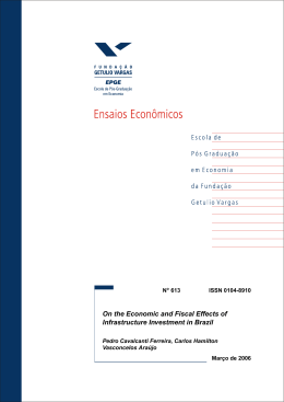
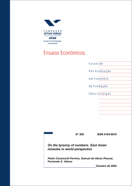
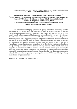
No 584
ISSN 0104-8910
What Happens After the Central Bank of
Brazil Increases the Target Interbank Rate by
1%?
Rubens Penha Cysne
Março de 2005
Os artigos publicados são de inteira responsabilidade de seus autores. As opiniões
neles emitidas não exprimem, necessariamente, o ponto de vista da Fundação
Getulio Vargas.
What Happens After the Central Bank of
Brazil Increases the Target Interbank Rate
by 1%?
Rubens Penha Cysney
March 15, 2005
Abstract
I start presenting an explicit solution to Taylor’s (2001) model, in
order to illustrate the link between the target interest rate and the
overnight interest rate prevailing in the economy. Next, I use Vector
Auto Regressions to shed some light on the evolution of key macroeconomic variables after the Central Bank of Brazil increases the target
interest rate by 1%. Point estimates show a four-year accumulated
output loss ranging from 0:04% (whole sample, 1980 : 1-2004 : 2; quarterly data) to 0:25% (Post-Real data only) with a …rst-year peak output response between 0:04% and 1:0%; respectively. Prices decline
between 2% and 4% in a 4-year horizon. The accumulated output
response is found to be between 3:5 and 6 times higher after the Real
Plan than when the whole sample is considered. The 95% con…dence
bands obtained using bias-corrected bootstrap always include the null
output response when the whole sample is used, but not when the data
is restricted to the Post-Real period. Innovations to interest rates explain between 4:9% (whole sample) and 9:2% (post-Real sample) of
the forecast error of GDP.
I am thankful to participants of workshops at the University of Chicago, for their
comments, and to Lutz Kilian, for making available some of the computer codes used in
this work. The usual disclaimer applies. Key Words: In‡ation, Brazil, COPOM, OpenMouth Operations, VAR, Vector Auto Regression, Bias-Corrected Bootstrap. CEL codes:
C15, E40, E50.
y
Professor at the Graduate School of Economics (EPGE/FGV) of the Getulio Vargas
Foundation and a Visiting Scholar at the Department of Economics of the University of
Chicago. E mail: [email protected].
1
1
Introduction
The current approach to monetary policy in Brazil is characterized by the
setting of two di¤erent targets: the in‡ation target and the targeting of the
rate at which …nancial institutions lend each other reserves overnight (the
interbank overnight interest rate target). In‡ation targeting was introduced
in Brazil in July/1999. Once the policy of controlling the nominal exchange
rate was abandoned by the Central Bank, at the beginning of 1999, a new
forward-looking regime enhancing transparency and the control of expectations emerged as the right thing to do.
The interbank-rate targeting is the main operational direct tool by means
of which in‡ation is kept equal or close to its target1 . It amounts in practice
to two coordinated policies conducted by the Central Bank. The …rst policy
regards the announcements of the interest-rate trends and/or targets for the
near future. It is a responsibility of the COPOM ("Comitê de Política Monetária"), which holds monthly meetings with this purpose. The second policy,
a responsibility of the Central Banks’s Trading Desk (Mesa de Operações da
DIOPE- Divisão de Operações), amounts to making daily open-market operations, in such a way that supply and demand for reserves intersect at an
interest rate equal or close to the desired target2 . There is no direct interference of the Central Bank, through its Trading Desk, on the interbank
rates.
Since the target interest rate is a crucial tool for the day-by-day policies
of the Central Bank, it is very important to know how changes in this rate
a¤ect other relevant macroeconomic variables such as the GDP, employment
and in‡ation.
Several elaborate econometric works have been produced by the Central
Bank of Brazil since the introduction of the In‡ation-Targeting regime, in
order to provide a technical background for the forecasts to be announced.
Among them, Bogdanski et al. (2000) concentrates on the dynamics involving interest rates, prices and output. These authors have concluded, using
structural models, that interest rate changes a¤ect aggregate demand in a
period of 3 to 6 months, output gap having an impact on in‡ation after 3
months. This makes a total around nine months between a policy action
based on the interest rate and curbing in‡ation. Tabak (2003) has found
1
Of course, the setting of this rate is also made with an eye towards the relative rates
of change of some monetary aggregates.
2
Martins (2003) and Barbosa (2005) are two available references describing the more
recent modus operandi followed by the Central Bank of Brazil concerning reserve requirements.
2
that, to a certain extent, market participants have been able to anticipate
some policy actions taken by the COPOM.
The VAR literature using Brazilian monetary data is not very vast. Pastore (1995, 1997) investigated in‡ation persistence and the passiveness of
money supply to the in‡ation rate. Fiorencio and Moreira (1999) used a
variable-coe¢ cient VAR to assess the e¤ectiveness of monetary policy in
di¤erent periods. Rabanal and Schwartz (2001) used 1995-2000 data to investigate output and money response to interest-rate shocks. Minella (2001,
2003) used monthly data from 1975 to 2000 to investigate the link between
interest rates, money and output and to compare three distinct periods of
the Brazilian economy.
This work intends to add to the Brazilian monetary literature in two
respects. First, a solution to Taylor’s model is presented as a tool in the
understanding of the link between the target interest rate and the overnight
interest rate. The main conclusion of this analysis, and the result that links
it to the Vector-Auto-Regression (VAR) analysis carried out in the second
part of this work is that, for reasonable values of the underlying parameters,
the convergence of interest rates to the target interest rate (which takes some
days) can be assumed to be practically negligible when compared to a time
interval of one quarter. By de…ning the time of the shock as that in which the
news are released, this allows for an interpretation of changes in the target
interest rate as shocks to interest rates.
The second part of the work carries out a VAR analysis with the purpose
of investigating how the dynamics of certain key macroeconomic variables
changes as a function of shocks to interest rates. More particularly, I will
be interested in the quantitative e¤ects of a 1% unexpected increase of the
target interest rate on prices, output and reserves. The estimation of the
four-year accumulated output response will receive particular attention.
As it is always the case in such analyses, all results are contingent on
the particular Cholesky decomposition chosen for the impulse-response estimation and on the assumption that the relevant sigma algebra on which
economic agents base their expectations is the one generated solely by the
series and lags used in the econometric estimations.
2
Taylor’s Model
3
Taylor (2001) o¤ers an easily readable model in which supply and demand
for bank reserves are written, respectively, as3 :
bt = bt
1
+ (rt
1
t 1 );
(1)
>0
and
bt =
(rt
Et rt+1 ) + "t ;
> 0; 0 <
<1
(2)
The …rst equation says that the supply of bank reserves (b) is increased,
at time (day) t; by (indirect) actions of the Desk, when the interest rate in
period t 1 is higher than the targeted interest rate ( ) at period t 1.
The second equation translates the demand of reserves by the banks. This
demand is positive when banks expect, conditionally on the information set
available at date t; that interest rates, corrected for the parameter ; will
increase from one day to another.
An important point in the understanding of Taylor’s model is that the
time period in which the variables in the model are accounted for (here, one
day) is much smaller than the time period in which banks must average their
reserves in order to comply with the reserve requirements set by he Central
Bank (usually, in Brazil, a period of ten business days). This implies that,
even with a partially lagged calculation of reserve requirements4 , banks still
have freedom enough to make (daily) adjustments of their reserve balances.
In terms of the classi…cation presented in Simonsen and Cysne (1995,
p. 656), this is a mixed system of stochastic di¤erence equations, since
there are autoregressive and forward looking components. By assuming that
information is not lost over time, (2) and the law of iterated expectations
lead to:
1
1X j
Et 1 bt+j + lim n Et 1 rt+n
Et 1 rt =
n!1
j=0
which shows how the value interest rates expected to prevail in the future
a¤ect the present interest rate.
Taylor (2001) does not explicitly solve the system of equations given by
(1) and (2).
3
I am using the term "bank reserves" as a shortening to "bank reserves held as deposits
in the Central Bank". This corresponds to what Taylor (2001) calls "fed balances".
4
Currently, in Brazil, as established by the Circular 2986, of June 23, 2000, reserve
requirements for each of two groups of banks are calculated taking into consideration
balances measured from business day 1 to business day 10, whereas mantained reserves
are averaged between business day 8 and business day 17. The system, therefore, cannot
be classi…ed as a lagged one, since there is an intersection of 3 business days (8, 9 and 10),
out of 10, between measurements and compliance. But it is close to that.
4
This can be easily done, under perfect foresight, in the case of an autonomous system ( t =
for all t): By writing:
zt =
bt
rt
;
1
A=
1
;
1
C=
0
(1) and (2) read:
(3)
zt+1 = Azt + C
The …xed point and the characteristic equation of (3) are, respectively,
(1
A) 1 C =
z = (I
and
f( ) =
1+
2
)
(4)
+
I will concentrate here only in the generic case in which the eigenvalues
are real and distinct. In this case the eigenvectors generate R2 and we can
consider the inverse of the matrix formed by the eigenvectors of A. The eigenvectors e1 = (e11; e12 ); e2 = (e21 ; e22 ) can be taken to be e1 = (1; (1 1 1 ) ) and
e2 = (1; (1 1 2 ) ); where 1 and 2 are the respective eigenvalues:By making
P = (e1 ; e2 ) and de…ning z^ = P 1 z; we have the system in diagonalized form:
1
z^t+1 = D^
zt + P
C
where D is a diagonal matrix having in the diagonal the eigenvalues 1 and
t
^
^t = c2 t2 ; the hats over the
2 . The general solution reads bt = c1 1 and r
variables having the obvious meaning.
Assuming that the parameters of the model generate j 1 j< 1 and j 2 j>
1; the transversality condition (saddle-path solution) implies c2 = 0: Using
(4) we have , in terms of the original variables of the system (since z = P z^):
b0
r0
1
=
1
1
(1
c1
0
1
1)
(1
2)
+
(1
)
which determines c1 as a function of b0 : The general solution then reads:
bt = (b0
(b0
rt =
1) ) t1
(
1) )
(1
1)
(
5
+
t
1
+ ;
(
1) ; t
(5)
0
t
1
(6)
Equations (5) and (6) determine the evolution of the endogenous variables
b and r , under di¤erent values of the parameters ; and ; when there are
changes of the target interest rate :
Taylor uses the parameter values = 0:9; = 0:3 and = 0:1 to draw
Figure 5 in his work. Figure 5 shows the evolution of interest rates when
the target interest rate changes from 0 to 0:5. The economy is supposed,
previously to period zero, and including period zero, to be in a steady state
with = r = 0 and b = b0 = 0 (the fact that b0 = 0 follows from equation
(2), since in the steady state rt = Et rt+1 ).
Note from (5) and (6) that when = 1; bt = b0 = 0 for all t; even though
the interest rate immediately adjusts to its new level. In other words, there
is no need of open market operations to change interest rates. This is what
Thornton (1999) and Guthrie and Wright (2000) referred to as "Open Mouth
Operations"5 .
Below I present some additional simulations of the solutions to (1) and
(2) using parameter values other than those used by Taylor:
Insert Figure 1 Here
Note that the higher the value of gamma (see Fur…ne (2000) for empirical
considerations regarding this parameter), the less time it takes for interest
rates and reserves to converge to the new steady states. Seeing the …gures
in Figure 1 as disposed like a 2x3 matrix, Figures 1x3 and 2x3 show the
instantaneous adjustment of interest rates and the invariance of the total
level of reserves when = 1; the case described above as the "open mouth"
case. Figure 2x2 corresponds exactly to Figure 5 in Taylor (2001).
Figure 2 below shows the evolution of the interbank rate (SELIC - Sistema
Especial de Liquidação e Custódia) and the target rate between 07/1999 and
01/2003:
Insert Figure 2 Here
Except for June/02, one can see in Figure 2 that the discrepancy between
the rates are usually very small.
3
Innovation Accounting
The previous section shows that, under reasonable assumptions regarding
the parameters of Taylor’s model, one can expect the overnight interest rate
5
See Martins (2003) for an analysis of the possibility of "open mouth" operations in
Brazil (this author calls it "efeito anúncio" (ad. e¤ect)).
6
to converge to the new target announced by the monetary authorities in a
period ranging from one to ten days.
From this section onwards, our time period will be of one quarter and
our horizon of analysis will take a total of four years. Since a ten-days
period under this horizon is practically negligible, one can associate news of
changes in the target rate with immediate shocks to interest rates. Besides
being supported by the logic behind Taylor’s model, this procedure can be
justi…ed by the data displayed in Figure 2.
With this in mind, from now on my purpose will be using impulseresponse and variance-decomposition analyses to study what happens to output, price level, and bank reserves, once interest rates are increased by one
percentile point (a hundred basis points)6 .
Initially, I derive qualitative considerations working with the whole sample period in which the macroeconomic variables under consideration are
available on a quarterly basis: 1980 : 1 2004 : 2. Later on in this section I
will use a subsample with data collected after the Real Plan (1994 : 2 2004 :
2).
3.1
Con…dence Bands: Bias-corrected Booststrap
As in Cysne (2004), here I use the con…dence bands for the impulse-response
functions based on Kilian’s (1998) bias-corrected bootstrap method.
The application of the standard bootstrap procedures to auto-regressive
models generates replicates which are necessarily biased, on account of the
small-sample bias of the estimators of the parameters. In order to deal
with this problem, speci…cally regarding the con…dence intervals for impulseresponse functions constructed from VAR estimates, Kilian (1998) proposed
correcting the bias prior to bootstrapping the estimate.
Monte Carlo studies carried out by this author (see p.222 in Kilian (1998))
show that the relative frequency at which the 95% con…dence interval covers
the true impulse response (in a model like the one used here) can be as low
as 50% when standard bootstrap methods are employed. The bias-corrected
bootstrap, on the other hand, presents a frequency around 90-95%7 .
In the estimations in levels and without trends, I employ Pope’s (1990)
closed-form solution to the bias of the estimators of the VAR. The theorem
reads:
6
For the e¤ect of changes in the target rate on the term structure of interest rates, in
the Brazilian case, see Tabak (2003).
7
The bias-corrected bootstrap detailed here has been primarily designed for stationary
VARs. However, Kilian (1998, section VI) demonstrates that this technique may still be
satisfactory, in practice, for nonstationary processes estimated in levels.
7
Theorem 1 (Pope (1990)): Let A^n be the least-squares estimator of A in
the m-dimensional AR(1): Xt = AXt 1 + Zt ; in which Xt and Zt are mx1
and A is mxm, based on a sample of size n. Make:
Cn (s) =
1
n
1
n 1
X
Ui s UiT
i=1
where Ut = Xt Xn ; Xn the sample mean. Suppose that, for some " > 0; E k
Cn (0) 1 k1+" (k : k states for the operator norm) is bounded as n ! 1
and that the innovations Zt are a martingale di¤erence sequence such that
all moments of Zt up to and including the sixth, conditional on the past,
are …nite and have values independent of t. Let G denote the conditional
covariance of Zt ; and suppose that k A k< 1: Then, as n ! 1; the bias
Bn = E A^n A is of the form:
Bn =
where b is given by:
h
b = G (I AT )
1
+ AT (I
b
+ O(n
n
(AT )2 )
1
+
3=2
X
(7)
)
(I
AT )
1
i
(0)
1
(8)
The sum is over eigenvalues of A;weighted by their multiplicities, and (j) =
T
EXt Xt+j
:
Proof. See Pope (1990).
The key point to note is that the bias for the bootstrap is re-estimated,
and new coe¢ cients are generated, in each resampling of the bootstrap.
3.2
Impulse-Response Functions
Let y, p, r, res and m denote, respectively, the logarithm of real GDP , the
logarithm of the price index, the short term (SELIC) interest rate, the logarithm of total (bank) reserves and the logarithm of M1 (means of payment).
The primitive data on p, m and r used here are from IBRE-FGV’s (Instituto
Brasileiro de Economia da Fundação Getulio Vargas) data bank. The quarterly GDP index and bank reserves are from IPEA (Instituto de Pesquisa
Econômica Aplicada.).
In all estimations in this work, the benchmark speci…cation used, regarding the ordering of the variables in the VAR, is the same as in Christiano et
al. (2000). Under this ordering, the information set assumed to be available
8
to the government at time t, when choosing the interest rate to target, includes the current and lagged values of y and p, as well as lagged values of
r, res and m. As a consequence of the ordering of the variables in the VAR
and of the Cholesky-orthogonalization assumption, neither the price level at
time t nor the GDP at time t are supposed to change as a consequence of a
contemporaneous interest-rate shock8 .
Results For The Model in Log Levels
Since the main goal here is to determine the interrelationships among
the variables, not the parameter estimates, in this subsection I follow Sims’s
(1980) and Doan’s (1992) suggestions9 and estimate the VAR in log levels .
A preliminary analysis of this data set has been carried out by Cysne
(2004). Using the Akaike and the Schwarz criteria10 , the model with 12 lags
outperformed the models with 4 and 8 lags.
For these reasons, regarding the estimation in levels and with the whole
data sample, I shall work here only with 12 lags. Figure 3 shows the response
of output and prices to an increase of one-percent deviation in interest rates,
using a VAR in log levels with a nonzero intercept and 12 lags:
Insert Figure 3 Here
The four sub-…gures in Figure 3 display the response of y, p, r and res
to a one percent increase in interest rates. All variables are in percentage
terms.
8
The fact that interest rates do not a¤ect output contemporaneously can be justi…ed by
previous work of Bogdanski et al (2000), who found, using structural models, that interest
rate changes a¤ect aggregate demand only after a period of 3 to 6 months.
9
See also Enders (1995, p. 301).
10
The maximum estimated absolute value of the eigenvalues of the A.R. matrix for 4, 8
and 12 lags are, respectively, 0.9815, 0.9829 and 0.9930. Reestimations of the VAR over
the same sample period lead to values of the Akaike Information Criterion, respectively,
for the model with 4, 8 and 12 lags, of 1.0969 1.1392 and -0.7527. This suggests the use of
the model with 12 lags. Even though we are dealing with a small sample, I also performed
a log-likelihood test under a null of 12 lags and an alternative of 8 lags. Asymptotically,
c = 2 (L12 L8) has a chi-square distribution with 100 (52 :4) degrees of freedom. The
value found was 367:2, con…rming the Akaike-Criterion option for 12 lags. Sims’ (1980)
bias-corrected version of this test calls for multiplying this statistics by (n1 n2 )=n1 ; where
n1 is the number of periods e¤ectively used in the regressions and n2 is the number of
parameters estimated in the equation with the highest number of parameters. This leads
to a new statistics s = 367:2 (86 61)=86 = 106. 74. The new p-value of 0:3049 does not
point out so de…nitely in favor of 12 lags.
9
As one can observe from the "r ! y" …gure, the product declines in the
…rst quarter to a maximum around 0:04% but recovers before the end of the
year11 . There is a rebound after the end of the …rst year and a subsequent
decline one quarter afterwards, which lasts for two years. A new rebound
after the third year, around 0:03%, is then followed by a further decline. Note
that the 95% con…dence bands include zero as a valid response throughout
the whole four-year period after the shock.
By aggregating the e¤ects over the GDP over a four-year horizon one
…nds an accumulated product decline around 0:07%; with lower and upper
bounds of 0:22% (GDP loss) and 0:20% (GDP gain):
Regarding the e¤ect on prices, as shown by Cysne (2004), there is a subtle
price puzzle in the …rst quarter after interest rates are increased. As of this
date, though, the e¤ect of interests on prices is of a four-year persistent
decline. In this case, a null response can be statistically rejected the …rst
year after the shock onwards.
Note that both output and prices are not contemporaneously a¤ected
by the shock in interest rates, a consequence of the economic assumptions
leading to the particular Cholesky decomposition used in the simulations.
Regarding the interest rate itself, the shock starts at the level of 1%, and
lasts around one quarter.
Finally, with respect to bank reserves, the contemporaneous e¤ect is negative, showing a decline around 0:4%. A rebound at the end of the …rst
quarter lasts for three quarters. After the end of the …rst year, the negative
e¤ect of interest rates on reserves lasts for the next three years, reaching a
maximum response of a decline around 3% at the fourteenth quarter after
the shock.
Trends and Unit Roots
It is a valid exercise checking how the results obtained by running the
VAR in log levels, without a trend, could change by using …rst di¤erences of
the nonstationary variables, or by the introduction of a time trend for the
regressions run in log levels. The respective impulse-response functions are
shown in Figures 4 and 5.
The results in di¤erences were obtained with four lags. To avoid clustering
the analysis, and since the objective of this section is primarily a comparison
with the estimation in log levels, I do not include con…dence bands.
11
Considering only the initial cycle shown by GDP, this is in agreement with Lisboa
(2004), who has argued that the short-run e¤ect, on output and employment, of an increase
of the target interest rate by the COPOM is temporary and lasts less than a year.
10
Insert Figure 4 and 5 Here
Regarding the estimation in log levels with a trend (the nonzero intercept
is assumed in all cases), the overall shape of the responses of all variables is
practically the same as in the case without trend. This could be expected,
given the large number of regressors in each equation. A quantitative di¤erence is that now the overall decline of product along the four years is found
to be 0:04%; a bit lower than the previous 0:07%:
Qualitatively, imposing unit root to the nonstationary variables leads to
some changes in the shape of the responses, but not signi…cant ones (Figure
5). The response of GDP is practically the same till the end of the …rst year.
There is initially a decline around 0.04%, followed by a recovery that lasts
till the end of the …rst year. In contrast to the estimation in levels, though,
the oscillations of output are now less subtle, remarkably between the …rst
an the fourth year. In both estimations output is back to its initial level forty
eight months after the initial shock.
The value of the accumulated decline in GDP over the four years now
amounts to 0:08%, a bit higher than the previous 0:07% regarding the estimation in levels without trend.
The price puzzle is a bit longer when the estimation is done with …rst
di¤erences, lasting between six to nine months, but always less than 0:2%.
The response of prices is steadily negative after the …rst year, repeating the
previous result.
Regarding interest rates, the shock initial 1% shock lasts for around six
months, as opposed to the previous three months of the estimation in levels
without trend. The …nal e¤ect at the end of the fourth year is a decline of
interest rates, repeating the estimation in levels.
The contemporaneous e¤ect on bank reserves is now positive (around
0:2%), in a subtle contrast with the estimation in levels. But after the end of
the …rst year, both estimations show a steady decline, which reaches a value
between 2% and 3% at the end of the fourth year.
3.3
Variance Decomposition
The purpose of this subsection is to measure the proportion of movements in
each of the sequences considered that can be attributed to its own shocks, or
to shocks to other variables. The same assumptions regarding the ordering
of the variables in the VAR used to obtain the impulse-response functions
apply here. The horizon considered is of four years. I provide variance
decomposition for the model in log levels only.
11
Insert Figure 6 Here
The results displayed in Figure 6 show that interest rates explain a relatively small share of the conditional variance of GDP (4:9%). Regarding
prices, interest rates, bank reserves and money, though, the e¤ect of shocks
to interest rates in explaining forecast errors is usually very relevant. Unexpected movements in interest rates account for around 39% of the variance of
prices, 35% of the variance of bank reserves and 36% of the variance of M1 .
Except for the e¤ect on GDP, shocks to interest rates play a more important
role in explaining forecast errors than shocks to money. Price and interestrate shocks, alone, explain around 80% of the forecast errors in reserves and
money.
4
Subsampling: Results For The Post-Real
Economy
The results obtained so far are satisfactory from a qualitative perspective but
may not be ideal for a description of the economy after the Real Plan. The
main reason is that as of 1994 : 2, macroeconomic variables evolved under a
very di¤erent pattern.
For instance, the standard deviations of the residuals in the estimation
of y, p, r, res and m are much higher when one considers the whole sample
than when one only includes Post-Real data. Following a signal-extraction
reasoning, the e¤ect on GDP of a 1% shock to interest rates after the Real
Plan should be higher than the one measured in a sample including data
both before and after the Plan. On the other hand, subsequent variations of
the interest rate should show an opposite pattern.
In this section I resample the data to include only the 1994:2 - 2004:2
(after Real) period and show that both of these facts indeed occur.
Since I am using quarterly data (there are no monthly estimates of GDP
in Brazil), this procedure leaves too little degrees of freedom to consider more
than four lags.
The product and interest-rate response are shown in Figure 7:
Insert Figure 7 Here
Note that, consistently with the fact that a one percent shock to interest
rate before the Real Plan should lead to a smaller response from the economy
than after the Real Plan, the new estimations show a much higher initial
12
decline of output (1%, as compared to 0:04% when the whole sample is used).
Although one must take into consideration that now we are using only 4 lags,
instead of 12, the initial decline of GDP is now much more resilient than in
the case of the full sample, lasting 1 12 years, instead of the initial 11 months.
In contrast to the estimations when the whole sample is used (see Figure
2), the 95% con…dence bands here do not include zero as a statistically valid
output response in the …rst six months after the shock.
The new accumulated output loss is 0:25%. Using the lower and upper
bands lead to a GDP variation of 3:54% and 3:48%.
Also as expected, interest rates now reach a lower bound around 0:4%,
much lower (in absolute value) than the 1:4% obtained when the pre-Real
data was included.
The new variance decomposition for the subsample 1994:2-2004:2 is presented in Figure 8.
Insert Figure 8 Here
The results displayed in Figure 8 show that interest rates in the more
recent period explain a larger share of the conditional variance of GDP (9:2%;
as opposed to the previous 4:9%). Unexpected movements in interest rates
now account for 2:14% of the variance of prices, 20% of the variance of bank
reserves and 6% of the variance of M1 . Shocks to money are now more
important than shocks to interest rates in explaining errors in the forecast of
all variables, except interest rates themselves.
5
Conclusions
Tis work has started with a short description of the two-target mechanism
that characterizes the state of monetary policy in Brazil after 1999. Next,
Taylor’s model for the determination of bank reserves and interest rates was
revised and simulated for di¤erent parameter values. A particular con…guration of the parameters has been noticed to lead to what is generally called
"open-mouth" operations, as opposed to "open-market" operations.
The second part of the paper provides a VAR analysis of the e¤ects over
output, interest rates, prices and bank reserves, of a 1% shock to the interest
rate caused by an unexpected increase of the target interest rate in the same
amount.
Point estimates show a four-year accumulated output loss ranging from
0:04% (estimation in log levels with a constant, using 1980 : 1-2004 : 2;
quarterly data) to 0:25% (estimation in log levels, without a constant, using
13
only Post-Real data) with …rst-year peak output response between 0:03%
and 1:0%; respectively. Prices always fall between 2% and 4% along the
4-year horizon. The accumulated output response is found to be between
3:5 and 6 times higher after the Real Plan than when the whole sample is
considered. In all estimations including the whole sample, the 95% con…dence bands obtained using bias-corrected bootstrap include the null output
response. The same, though, does not happen when one uses only Post-Real
data. Innovations to interest rates explain between 4:9% (whole sample) and
9:2% (post-Real sample) of the forecast error of GDP.
Qualitatively, a negative correlation between the target rate and prices,
as well as between the target rate and output (or bank reserves) is robust to
the method of estimation (if with or without a constant and if in levels or in
…rst di¤erences) and to a subsampling that includes only the data after the
Real Plan.
References
[1] Barbosa, Fernando H. and Ribeiro, Edmundo M. de O. (2005): "A
Demanda de Reservas Bancárias no Brasil". Ensaio Econômico da EPGE
n. 581, FGV-R.J.
[2] Bogdanski, J., Tombini, A. T. and Werlang, S. R da C. , 2000, "Implementing In‡ation Targeting in Brazil", Working Paper Series 1, Central
Bank of Brazil.
[3] Christiano, Lawrence, Martin Eichenbaum and Charles Evans, 2000,
“Monetary policy shocks: what have we learned and to what end?” In
Michael Woodford and John Taylor, eds., Handbook of Macroeconomics
North Holland.
[4] Cysne, R. P., 2004, "Is There a Price Puzzle in Brazil? An Application
of Bias-Corrected Bootstrap". Ensaio Economico da EPGE n. 577.
[5] Doan, Thomas A., 1992, "RATS User’s Manual", Evanston, Ill. Estima.
[6] Enders, W., 1995, "Applied Econometric Time Series", Wiley Series in
Probability and Mathematical Statistics, New York, USA.
[7] Fiorencio, Antonio, and Ajax R. B. Moreira (1999), “Latent Indexation
and Exchange Rate Passthrough”, Rio de Janeiro, IPEA, Texto para
Discussão no. 650, Jun.
14
[8] Fur…ne, C. H., -(2000), "Interbank payments and the Daily Federal
Funds Rates". Journal of Monetary Economics 46:535-553.
[9] Guthrie, G. and Wright, J., 2000, "Open Mouth Operations", Journal
of Monetary Economics 46 (2000) 489}516.
[10] Kilian, L., 1998, "Small-Sample Con…dence Intervals for ImpulseResponse Functions". The Review of Economics and Statistics, 80, 218230.
[11] Lisboa, M. 2004, Interview, Jornal Folha de São Paulo, 23/10/2004,
Page B-4.
[12] Martins, M. G., (2003). "Efeito Anúncio da Política Monetária: A
Experiência Brasileira". Dissertação de Mestrado. EPGE/Fundação
Getúlio Vargas.
[13] Minella, A., (2001), "Monetary Policy and In‡ation in Brazil (19752000): a VAR Estimation", Working Paper Series 33, Central Bank of
Brazil.
[14] Minella, A., (2003), "Monetary Policy and In‡ation in Brazil (19752000): a VAR Estimation", Rev. Bras. Econ. vol.57 no.3 Rio de Janeiro.
[15] Pastore, A¤onso C. (1995), "Dé…cit Público, a Sustentabilidade do
Crescimento das Dívidas Interna e Externa, Senhoriagem e Inzação:
uma Análise do Regime Monetário Brasileiro", Revista de Econometria,
vol. 14, no. 2, pp. 177-234.
[16] Pastore, A¤onso C. (1997), “Passividade Monetária e Inércia”, Revista
Brasileira de Economia, vol. 51, no. 1, pp. 3-51, Jan.-Mar.
[17] Pope, Alun L., 1990, "Biases of Estimators in Multivariate NonGaussian Autoregressions". Journal of Time Series Analysis 11, 249–
258.
[18] Rabanal, Pau, and Gerd Schwartz (2001), “Testing the Ex
oectiveness
of the Overnight Interest Rate as a Monetary Policy Instrument”, In:
International Monetary Fund, Brazil: selected issues and statistical appendix, IMF Country Report No. 01/10, Washington, D.C., Jan.
[19] Simonsen, M. H. and Cysne, Rubens P. (1995): “Macroeconomia, Second Edition”. Editora Atlas, São Paulo.
15
[20] Sims, Christopher A., 1980, "Macroeconomics and Reality", Econometrica, 48:1-48.
[21] Tabak, B. M., 2003: "Monetary Policy Surprises and the Brazilian Term
Structure of Interest Rates", Working Paper Series n. 30, Central Bank
of Brazil
[22] Taylor, J. 2001, "Expectations, Open Market Operations, and Changes
in the Federal Funds Rate". Federal Reserve Bank of St. Louis.
[23] Thornton, D. L., 1999, "The Relationship Between the Federal Funds
Rate and the Fed’s Federal Funds Rate Target: Is It Open Market or
Open Mouth Operations?", Working Paper 1999-022B, Federal Reserve
Bank of St. Louis.
16
rho → b
0
0
1
gamma=.5
gamma=.9
gamma=1
-0.02
0.5
b
-0.005
-0.04
0
-0.01
-0.06
-0.08
0
5
t
-0.5
-0.015
10
0
5
10
-1
0
5
10
0
5
10
rho → r
0.5
0.5
0.4
0.4
0.4
0.3
0.3
0.3
0.2
0.2
0.2
0.1
0.1
0.1
r
0.5
0
0
5
10
0
0
5
10
0
Figure 1: Response of Reserves and Interest Rates to a Unanticipated 0.5%
Increase in the Targe Rate
17
Figure 2: Interbank Rate and Targe Rate (Flat)
18
Source: Martins (2003)
r→y
r→p
2
12 lags
0.1
0.05
0
0
-2
-0.05
-4
-0.1
-6
1
2
3
4
1
r→r
2
3
4
3
4
r → res
2
2
0
1
0
-2
-1
-4
-2
1
2
3
4
1
2
Figure 3: Impulse-Response Functions, VAR in Levels Without Trend. Sample: 1980:1-2004:2
19
r→y
r→p
2
12 lags
0.1
0.05
0
0
-2
-0.05
-4
-0.1
-6
1
2
3
4
1
r→r
2
3
4
3
4
r → res
2
2
0
1
0
-2
-1
-4
-2
1
2
3
4
1
2
Figure 4: Impulse-Response Functions, VAR in Levels With a Trend. Sample: 1980:1-2004:2
20
r→y
0.04
r→p
1
4 lags
0.02
0
0
-1
-0.02
-2
-0.04
-3
-0.06
1
2
3
4
1
r→r
2
3
4
3
4
r → res
1
1
0
0.5
0
-1
-0.5
-2
-1
-3
1
2
3
4
1
2
Figure 5: Impulse-Response Functions, VAR in First Di¤erences. Sample:
1980:1-2004:2
21
Figure 6: Variance Decomposition, Model in Log Levels
r→y
r→r
4 lags, 1994-2004
2
1.5
1.5
1
1
0.5
0.5
0
0
-0.5
-1
-0.5
-1.5
-2
-1
1
2
3
4
1
2
3
4
Figure 7: Response GDP and Interest-Rate Response to a 1% Increase of the
Target Interest Rate, Subsample 1994:2-2004:2. Estimation in Levels.
Figure 8: Variance Decoposition, Model in Log Levels, Subsample 1994:22004:2
22
Últimos Ensaios Econômicos da EPGE
[565] Marcelo Casal de Xerez e Marcelo Côrtes Neri. Desenho de um sistema de
metas sociais. Ensaios Econômicos da EPGE 565, EPGE–FGV, Set 2004.
[566] Paulo Klinger Monteiro, Rubens Penha Cysne, e Wilfredo Maldonado. Inflation
and Income Inequality: A Shopping–Time Aproach (Forthcoming, Journal of
Development Economics). Ensaios Econômicos da EPGE 566, EPGE–FGV, Set
2004.
[567] Rubens Penha Cysne. Solving the Non–Convexity Problem in Some Shopping–
Time and Human–Capital Models. Ensaios Econômicos da EPGE 567, EPGE–
FGV, Set 2004.
[568] Paulo Klinger Monteiro. First–Price auction symmetric equlibria with a general
distribution. Ensaios Econômicos da EPGE 568, EPGE–FGV, Set 2004.
[569] Samuel de Abreu Pessôa, Pedro Cavalcanti Gomes Ferreira, e Fernando A. Veloso. On The Tyranny of Numbers: East Asian Miracles in World Perspective.
Ensaios Econômicos da EPGE 569, EPGE–FGV, Out 2004.
[570] Rubens Penha Cysne. On the Statistical Estimation of Diffusion Processes –
A Partial Survey (Revised Version, Forthcoming Brazilian Review of Econometrics). Ensaios Econômicos da EPGE 570, EPGE–FGV, Out 2004.
[571] Aloisio Pessoa de Araújo, Humberto Luiz Ataide Moreira, e Luciano I. de Castro Filho. Pure strategy equilibria of multidimensional and Non–monotonic auctions. Ensaios Econômicos da EPGE 571, EPGE–FGV, Nov 2004.
[572] Paulo César Coimbra Lisbôa e Rubens Penha Cysne. Imposto Inflacionário
e Transferências Inflacionárias no Mercosul e nos Estados Unidos. Ensaios
Econômicos da EPGE 572, EPGE–FGV, Nov 2004.
[573] Renato Galvão Flôres Junior. Os desafios da integração legal.
Econômicos da EPGE 573, EPGE–FGV, Dez 2004.
Ensaios
[574] Renato Galvão Flôres Junior e Gustavo M. de Athayde. Do Higher Moments
Really Matter in Portfolio Choice?. Ensaios Econômicos da EPGE 574, EPGE–
FGV, Dez 2004.
[575] Renato Galvão Flôres Junior e Germán Calfat. The EU–Mercosul free trade
agreement: Quantifying mutual gains. Ensaios Econômicos da EPGE 575,
EPGE–FGV, Dez 2004.
[576] Renato Galvão Flôres Junior e Andrew W. Horowitz. Beyond indifferent players:
On the existence of Prisoners Dilemmas in games with amicable and adversarial
preferences. Ensaios Econômicos da EPGE 576, EPGE–FGV, Dez 2004.
[577] Rubens Penha Cysne. Is There a Price Puzzle in Brazil? An Application of
Bias–Corrected Bootstrap. Ensaios Econômicos da EPGE 577, EPGE–FGV,
Dez 2004.
[578] Fernando de Holanda Barbosa, Elvia Mureb Sallum, e Alexandre Barros da Cunha. Competitive Equilibrium Hyperinflation under Rational Expectations. Ensaios Econômicos da EPGE 578, EPGE–FGV, Jan 2005.
[579] Rubens Penha Cysne. Public Debt Indexation and Denomination, The Case
of Brazil: A Comment. Ensaios Econômicos da EPGE 579, EPGE–FGV, Mar
2005.
[580] Renato Galvão Flôres Junior, Germán Calfat, e Gina E. Acosta Rojas. Trade and
Infrastructure: evidences from the Andean Community. Ensaios Econômicos da
EPGE 580, EPGE–FGV, Mar 2005.
[581] Edmundo Maia de Oliveira Ribeiro e Fernando de Holanda Barbosa. A Demanda
de Reservas Bancárias no Brasil. Ensaios Econômicos da EPGE 581, EPGE–
FGV, Mar 2005.
[582] Fernando de Holanda Barbosa. A Paridade do Poder de Compra: Existe um
Quebra–Cabeça?. Ensaios Econômicos da EPGE 582, EPGE–FGV, Mar 2005.
[583] Fabio Araujo, João Victor Issler, e Marcelo Fernandes. Estimating the Stochastic
Discount Factor without a Utility Function. Ensaios Econômicos da EPGE 583,
EPGE–FGV, Mar 2005.
[584] Rubens Penha Cysne. What Happens After the Central Bank of Brazil Increases
the Target Interbank Rate by 1%?. Ensaios Econômicos da EPGE 584, EPGE–
FGV, Mar 2005.
[585] Gustavo Gonzaga, Naércio Menezes Filho, e Maria Cristina Trindade Terra.
Trade Liberalization and the Evolution of Skill Earnings Differentials in Brazil. Ensaios Econômicos da EPGE 585, EPGE–FGV, Abr 2005.
[586] Rubens Penha Cysne. Equity–Premium Puzzle: Evidence From Brazilian Data.
Ensaios Econômicos da EPGE 586, EPGE–FGV, Abr 2005.
[587] Luiz Renato Regis de Oliveira Lima e Andrei Simonassi. Dinâmica Não–Linear
e Sustentabilidade da Dı́vida Pública Brasileira. Ensaios Econômicos da EPGE
587, EPGE–FGV, Abr 2005.
[588] Maria Cristina Trindade Terra e Ana Lucia Vahia de Abreu. Purchasing Power
Parity: The Choice of Price Index. Ensaios Econômicos da EPGE 588, EPGE–
FGV, Abr 2005.
[589] Osmani Teixeira de Carvalho Guillén, João Victor Issler, e George Athanasopoulos. Forecasting Accuracy and Estimation Uncertainty using VAR Models with
Short– and Long–Term Economic Restrictions: A Monte–Carlo Study. Ensaios
Econômicos da EPGE 589, EPGE–FGV, Abr 2005.