HYSTERESIS VS NAIRU & CONVERGENCE VS DIVERGENCE:
THE BEHAVIOR OF REGIONAL UNEMPLOYMENT RATES IN BRAZIL
Fábio Augusto Reis Gomesa, ∗, Cleomar Gomes da Silvab,##
a
João Pinheiro Foundation, School of Government and Center for Research in International
Economics
b
Getulio Vargas Foundation, São Paulo School of Economics and Center for Research in
International Economics
Abstract
In this article we examine the Hysteresis effect in the unemployment rates of six metropolitan areas in Brazil
- São Paulo, Rio de Janeiro, Belo Horizonte, Porto Alegre, Salvador e Recife - as well as in the aggregate
unemployment rate. The validity of the Hysteresis hypothesis is examined through the use of both ADF and
unit root break tests. Our results show that the phenomenon occurs in all regions, except in Rio de Janeiro,
and in Brazil as a whole. As a consequence, there is a clear rejection of the NAIRU hypothesis. These results
indicate a high persistence in the unemployment rates. Therefore, we go one step further and investigate
whether the five metropolitan regions, which are characterized by the Hysteresis effect, present stochastic
convergence as well. Our findings suggest that only Porto Alegre does not exhibit stochastic convergence.
Keywords: unemployment, NAIRU, Hysteresis, convergence, structural breaks.
JEL Classification: C12, C22, J64
∗
Corresponding author: Escola de Governo Professor Paulo Neves de Carvalho, Fundação João Pinheiro.
Alameda das Acácias 70, sala 143B, São Luiz. Belo Horizonte, MG - CEP: 31275-150, Brasil. E-mail:
[email protected] (Fábio Gomes).
#
The author gratefully acknowledges CNPQ for financial support.
1.
Introduction
There is no doubt unemployment has been a recurrent problem in several countries
and it is a much bigger matter nowadays than it used to be some decades ago. As a result,
unemployment is now a major source of concern among policymakers and society as a
whole. This is not different in Brazil and it even seems to have deeper roots in this country
due to, among many other factors, a series of failed economic stabilization plans in the
1980s and in the beginning of the 1990s, the opening of the Brazilian economy as well as a
tight conduct of monetary policy towards the end of the 1990s.
Theoretically, there are two main hypotheses related to the explanation of
unemployment. The first one is the non-accelerating-inflation rate of unemployment
(NAIRU) hypothesis, which characterizes unemployment dynamics as a stationary process
and, therefore, consistent with a stable inflation rate. In other words, the NAIRU states that
the unemployment rate should oscillate about a long-run steady state. The second one is the
Hysteresis hypothesis, which states that movements in unemployment might have a longterm persistence once it is affected permanently by cyclical fluctuations.1
The NAIRU hypothesis was brought to light by the seminal articles of Phelps
(1967) and Friedman (1968) and, over the 1950s and 1960s, it was able to provide
sufficient explanation for the behavior of unemployment. However, it began to be
questioned in the following decades due to constant movements observed in the
unemployment rates around the world. This resulted in the Hysteresis hypothesis, which
had one of its first statements in Blanchard and Summers (1986), who were concerned
about the phenomenon in Europe.
As the Hysteresis theory evolved, several articles started to empirically test it and
compare the results with the NAIRU hypothesis. In order to do this, researchers make use
of time series econometrics and, more specifically, checking the order of integration of the
unemployment rates. The reason is straightforward. The natural rate theory can be
supported by level stationarity of the series whereas the presence of a unit root
1
Phelps (1994) describes a third theory of unemployment suggesting that most shocks to unemployment are
temporary with occasional (but permanent) changes in the natural rate. As a result, the unemployment rate
can be defined as a stationary process around a small number of (permanent) structural breaks (Lee,
Strazicich & Tieslau, 2001). In other words, this can be seen as an extension of the NAIRU hypothesis as it
accounts for the possibility of occasional changes in the long-run steady state unemployment rate. Therefore,
the unemployment rate is stationary, as in the traditional version of NAIRU, but around a broken trend. In
both cases, the unemployment rate does not present a prominent degree of persistence, as opposed to the
hysteresis hypothesis. For that reason, in this paper we will refer to the NAIRU theory even in the case of
structural changes in the unemployment rate.
2
characterizes the Hysteresis hypothesis. Arestis & Mariscal (1999), Lee, Strazicich &
Tieslau (2001) and Camarero and Tamarit (2004) are some of the works that apply this
methodology, each one with some peculiarities but all of them for OECD countries, as it
will be seen in the next section.
So far, we have talked about a literature that looks at unemployment from a
national point of view. However, analyzing the nationwide unemployment rate may hide
important disparities amongst regional unemployment rates, particularly in Brazil, which
has continental dimensions and significant development differentials among its cities.
Indeed, the aggregate unemployment rate in Brazil, released by the National Bureau of
Geography and Statistics (IBGE), is a weighted average of the unemployment rates of the
six major metropolitan areas (São Paulo, Rio de Janeiro, Belo Horizonte, Recife, Salvador,
Porto Alegre), each one with peculiarities that ought to be taken into consideration.
The importance of studying regional unemployment is well discussed in Marston
(1985), who gives a clear explanation of the so-called compensation theory and examines
unemployment rate differentials among American cities. For the Brazilian case, Oliveira &
Carneiro (1999) look for a possibility to establish a long-run relationship between
unemployment rates of Brazilian States and the national rate. Corseuil, Gonzaga & Issler
(1999) also investigate short run and long run unemployment movements across the
already mentioned six metropolitan regions in Brazil.
Given the magnitude of the subject, it is of utmost significance to investigate the
unemployment rates in the six major Brazilian metropolitan areas. Therefore, the purpose
of this paper is twofold. First of all, we will test the both Hysteresis and NAIRU hypotheses
for both the aggregate and regional unemployment rates in Brazil. The econometric
methodology applied for testing the validity of the Hysteresis hypothesis is both standard
Augmented Dickey-Fuller (ADF) tests as well as the endogenous one and two break LM
unit root tests proposed in Lee and Strazicich (1999, 2003). The second aim of the article,
which is in line with the regional unemployment literature, is a long run analysis that will
enable us to check the convergence hypothesis for the regional unemployment series. The
methodology employed is a straightforward extension to the unemployment case of the
stochastic convergence proposition put forward by Carlino and Mills (1993), who study
income convergence across US regions.
Our results show that the hysteresis phenomenon occurs in all regions, except in
Rio de Janeiro, and in Brazil as a whole. This result indicates a high persistence in the
Brazilian unemployment series, which is a consequence of many factors such as several
3
failed economic policies. As for the convergence test, our findings suggest that São Paulo,
Belo Horizonte, Salvador and Recife present the stochastic convergence, which implies
that Porto Alegre’s unemployment rate differential remains in the long-run.
The remainder of the paper is organized as follows. Section 2 revises the literature
on NAIRU versus Histeresis hypothesis and describes our econometric methodology on the
subject. Section 3 revises the literature on convergence and details the econometric
approach on this topic. Section 4 presents the data and its descriptive analysis as well as an
overview of the unemployment problem in Brazil. Section 5 describes the results and
section 6 concludes.
2.
NAIRU versus Hysteresis: Literature and Econometric Approach
As mentioned above, Blanchard and Summers (1986) were worried about the
hysteresis phenomenon in Europe in the 1980s. The authors argued that anything which
increased the actual rate of unemployment for a sufficient length of time - a sustained
increase in real interest rates induced by monetary policy, for instance - was likely to affect
both the actual and the natural rate of unemployment.
Following this important article, several articles began to make empirical analyses
on the subject.2 For instance, using the ADF unit root test Neudorfer, Pichelmann &
Wagner (1990) examine the Hysteresis hypothesis for Austria and Jaeger & Parkinson
(1994) analyze the unemployment rates in the U.K., the USA, Canada and Germany. Both
works did not reject the null hypothesis of a unit root and, consequently, the Hysteresis
theory. As a benchmark examination, we also apply the ADF using the following
specification:
2
To the best of our knowledge there are no articles comparing hysteresis and NAIRU hypothesis for the
Brazilian case. Some works attempt only to find the Brazilian NAIRU. For instance, Portugal & Madalozzo
(2000) use two different unemployment rate series, which belong to the National Bureau of Geography and
Statistics (IBGE) and the Worker’s Union Bureau of Statistics (DIEESE), for the period between 1982:3 and
1997:3. For the IBGE’s data they find a NAIRU varying from 3.05% in the third quarter of 1986 to 9.21% in
the fourth quarter of 1989. The use of DIEESE’s series data results in a constant NAIRU of 10.3%. The
authors also suggest that the actual rate of unemployment converges to the NAIRU in the period
995.3/1997.3, reaching its long-term equilibrium level at some point during that period. Lima (2000) also
estimates the Brazilian NAIRU using IBGE’s data(1982.1/1999.3). The author works with ARCH residuals
and Markov-switching regime and concludes that the estimates of the NAIRU are very imprecise. These two
works show that hysteresis hypothesis may be the case for the Brazilian data once no result is robust enough
to confirm the NAIRU hypothesis.
4
k
∆U t = µ + β t + αU t −1 +
j =1
c j ∆U t − j + ε t
(1)
where Ut is the unemployment rate, µ and t are the constant term and the linear trend,
respectively.3
However, since Perron (1989), it is well known that ADF tests can fail to reject a
false unit root due to misspecification of the deterministic trend. In fact, Perron (1989,
1997) and Zivot and Andrews (1992) extend the ADF test considering an exogenous and
an endogenous break in an attempt to avoid this problem. Indeed, Mitchell (1993) performs
Perron’s unit root tests and his results also support the unit root hypothesis and hysteresis
for several OECD nations. Arrufat et alli. (1999) perform unit root tests with structural
breaks, based on Zivot and Andrews’ methodology, for the Argentine rate of
unemployment as well as for 24 urban locations. Their results reject the unit root null
hypothesis for 15 locations, including the nation-wide rate of unemployment.4
Lumsdaine and Papell (1997) extended Zivot and Andrews’s test allowing for two
breaks in level and trend. Arestis and Mariscal (1999) apply this methodology for 26
OECD countries and show a rejection of the Hysteresis hypothesis for the majority of the
nations. However, these extensions of the ADF test including one or two breaks also have
some drawbacks once they derive their critical values assuming no break(s) under the unit
root null hypothesis, which lead to a spurious rejection of the null hypothesis in the
presence of a unit root with breaks, as discussed by Lee and Strazicich (1999, 2003). In
order to avoid such problems, the authors propose an endogenous one/two-break LM unit
root tests, whose properties are unaffected by breaks under the null, in contrast to the ADFtype tests. Therefore, in addition to using the ADF test, we apply this LM test, whose
methodology is as follows.5
According to the LM (score) principle, a unit root test statistic can be obtained from
the following regression:
~
∆U t = d '
∆Z t + φS t −1 +
k
i =1
~
γ i ∆S t −i + ε t
(2)
Where:
3
Following Ng and Perron (1995) we define a k-max to choose k and use the (approximate) 10% value of the
asymptotic normal distribution, 1.645, to assess the significance of the last lag.
4
For the US case, Staiger, Stock and Watson (1997) suggest that the evidence doesn’t support the Hysteresis
hypothesis. They argue that, although there have been some shifts, they have been minor over the last 3
decades
5
Due to space limitations we present the two-break case. For the one break test methodology see Lee and
Strazicich (1999).
5
i) ∆St −i , i = 1,..., k , terms are included as necessary to correct for serial correlation;6
~
ii) S t is a de-trended series such that:
~
~
S t = U t −ψ~ x − Z t δ , t = 2,
(3)
,T
~
iii) δ is a vector of coefficients in the regression of ∆U t on ∆Z t ;
~
iv) ψ~ x = U 1 − Z1δ , where Z t is a vector of exogenous variables defined by the data
generating process;
v) U 1 and Z1 are the first observations of U t and Z t , respectively;
[
]
′
vi) Considering 2 changes in level and trend Z t is described by 1, t , D1t , D2t , DT1∗t , DT2∗t ,
where:
a) D jt = 1 for t ≥ TBj + 1 , j = 1,2, and zero otherwise; b) DT jt∗ = t for t ≥ TBj + 1 , j = 1, 2,
and zero otherwise; c) TBj stands for the time period of the breaks. Note that the test
′
regression (2) involves ∆Z t instead of Z t so that ∆Z t becomes [1, B1t , B2t , D1t , D2t ] ,
where B jt = ∆D jt and D jt = ∆DT jt∗ , j = 1,2 .
The unit root null hypothesis is described in equation (2) by φ = 0 and the test
~
statistic is defined is given by: ρ~ = T ⋅ φ ,
τ = t-statistic for the null hypothesis φ = 0
(4)
To endogenously determine the location of the two break points TBj in each time series, we
use a similar procedure used in the “minimum LM test”, that is, a grid search is utilized to
determine the break where the t-test statistic is minimized:
LM τ = Inf τ ( λ )
(5)
There is a repeated procedure at each combination of break points (λ j = TBj / T , j = 1,2 )
over the time interval [.1T,.9T] where T is the sample size. As shown in Lee and Strazicich
(2003), critical values for this model depend on the location of breaks ( λ j = TBj T , j = 1,2 ).
As a result, we utilize critical values that correspond to the location of the breaks.
6
See footnote 3.
6
Finally, Lee, Strazicich & Tieslau (2001) study the validity of the Hysteresis
hypothesis with yearly unemployment rate data from 17 OECD countries for the period
between 1955 and 1999. The authors employ a panel LM unit root test which allows for
heterogeneous structural change and find a strong rejection of the hypothesis. More
recently, Camarero and Tamarit (2004) studied a panel of 19 OECD countries and, for that,
applied a sequential procedure based on two multivariate ADF test-type panel unit root
tests in a SURE framework. Their results strongly reject the joint null of Hysteresis.7
3.
Regional Unemployment and Convergence: Literature and Econometric
Approach
Regardless of the integration order of the series, it is imperative to study the
regional unemployment series, i.e., it is important to study whether unemployment rates
among different regions have got something in common which attracts them in the long
run. Indeed, convergence matters especially when the series are integrated. In other words,
if the Hysteresis hypothesis is the case, which indicates that there is no mean reversion in
the series, they might also present some convergence pattern. For that reason, looking for
disparities amongst regional unemployment rates as well as seeing if there is any process
of convergence amongst them is a crucial investigation for Brazil once, as mentioned
previously, it has got continental dimensions and several peculiarities between regions.
Consequently, our study will focus on the unemployment rates of the country’s six major
metropolitan areas - São Paulo (SP), Rio de Janeiro (RJ), Belo Horizonte (BH), Recife,
Salvador, Porto Alegre (PA).
The importance of studying regional unemployment is well discussed in Marston
(1985), who gives a clear explanation of the so-called compensation theory, which predicts
that in equilibrium all individuals have the same utility level, and so areas more attractive
could have a larger unemployment rate. The author examines unemployment rate
differentials among American cities and his findings show that disturbances to the steadystate relationship among unemployment rates of important US metropolitan regions are
likely to disappear because of mobility within a particular year. Blanchard and Katz (1992)
go one step further and say that when jobless individuals move to other areas to look for
work there is an adjustment of the labor market towards a long-run equilibrium, i.e., there
will be convergence of regional unemployment rates. The authors analyze the dynamics of
7
We decided not to apply panel tests because we use only seven cross-section units.
7
the American regional unemployment but don’t find a strong indication for stationarity of
the rates and attribute the weak results to the tests used.
Jimeno & Bentolila (1998) look at the Spanish regional unemployment persistence.
They show that regional wages, and relative unemployment and participation rates, are
very persistent in Spain, while employment growth rates are not. Wu (2003) studies the
Chinese regional unemployment persistence through a panel data approach. According to
the author, three empirical findings are suggested. Firstly, provincial relative
unemployment shows a greater persistence when compared to the nationwide
unemployment rate. Secondly, total unemployment is more persistent than youth
unemployment. Thirdly, the region with the highest provincial unemployment rate is the
one with the lowest persistence of regional unemployment. Finally, the author finds out
that Chinese jobseekers are usually driven to the private sector, which has helped reduce
unemployment persistence. Bayer & Juessen (2004) analyze West German Regional
Unemployment Rates and also apply unit-root tests that allow for structural breaks. For
three of the ten federal states, and for Germany as a whole, the null hypothesis of a random
walk cannot be rejected. The authors also find a strong evidence for convergence and that
the speed of this convergence is very high.
As for the analysis of provincial unemployment in Brazil, Corseuil, Gonzaga &
Issler (1999) investigate short run and long run unemployment movements across the
mentioned six metropolitan regions in Brazil. The authors find evidence that, with an
exception for the Recife metro area, aggregate components are relevant for regional
unemployment rates. They also categorize short and long run comovements among the
other five unemployment rates and the national unemployment rate. In addition to that, the
article makes a decomposition of the unemployment series on permanent and temporary
elements. The former follows very closely the respective unemployment rates, which is an
indication of high persistence of the disturbances that influence the regional unemployment
rates.
Oliveira & Carneiro (2001) also look for a possibility to establish a long-run
relationship between states and national rates of unemployment. Two econometric
techniques are used: The Engle-Granger cointegration analysis and the Unrestricted Error
Correction Model. Their findings suggest that, in general, the states and the nation-wide
unemployment rates have similar dynamics, but with permanent differences in the long
run. If we suppose that the states have different attractiveness level, this result is consistent
8
with Marston (1985) prediction that in equilibrium all individuals have the same utility
level, and so areas more attractive could have a larger unemployment rate.
If this is the case, it is important to examine this topic for our data set. Therefore,
besides examining the Hysteresis hypothesis for Brazil, this paper makes use of the
stochastic convergence concept, developed by Carlino and Mills (1993), and studies the
progression of provincial discrepancies in unemployment rates within Brazil. Carlino and
Mills’ (1993) approach, which was originally developed to study per capita income
convergence among US regions, is based on the following idea: If per capita income of
different regions is converging, then their income should not diverge arbitrarily and,
consequently, the relative income – the (ln) ratio of region “i” income and the mean
income – should be stationary, which can be test by a unit root test.8
In other words, the aim is to extend the authors’ approach and apply it to the
relative unemployment of those regions that present hysteresis. Thus, the first step consists
in defining the relative unemployment rate of region i, uit, as the (ln) ratio of
unemployment rate Ui and the average unemployment rate of the regions, such that,
u it = ln U it
I
i =1
U it I
(6)
Stochastic convergence is defined as the (ln) of the unemployment rate from one
region relative to the region’s average, uit, being stationary. In other words, under
stochastic convergence, shocks to a region’s relative unemployment are temporary. For
each area, we examine the null hypothesis that unemployment is diverging by testing for a
unit root in uit. Failure to reject the unit root’s null hypothesis indicates evidence against
stochastic convergence. The stochastic convergence is examined using the same unit root
procedure applied to the hysteresis hypothesis, i.e., ADF tests and Lee and Strazicich’s
(1999, 2003) framework, whose methodology has already been described previously.
4
Data, Overview, and Descriptive Analysis
In this section the aim is to present the data used in the article. After that, there will
be an overview of the unemployment dynamics in Brazil in the 1980s, 1990s and
8
While Carlino and Mills apply unit root tests with a exogenous break, Loewy and Papell (1996),
Tomljanovich and Vogelsang (2002) and Strazicich et al. (2004) refine their approach using endogenous
break unit root tests.
9
beginning of the present decade. Finally, a descriptive analysis of the series will be
outlined.
4.1
Data
The data used in the analysis are the seasonally adjusted monthly rates of open
unemployment for the six major Brazilian metropolitan areas (São Paulo Rio de Janeiro,
Belo Horizonte, Recife, Salvador e Porto Alegre) and the nation-wide rate as well. The
source is the Monthly Employment Survey (Pesquisa Mensal de Emprego) from the
National Bureau of Geography and Statistics (IBGE), from 1981:01 to 2002:12, totaling
264 observations.9 It should be remarked that the aggregate rate of unemployment for
Brazil corresponds to the weighted average of the regional rates, relative to the
economically active population of each metropolitan region.
4.2
Overview of the Brazilian Unemployment
The beginning of the 1980’s definitely represents a turning point in the Brazilian
economy. The so-called “economic miracle” of the 1970s had come to an end with
negative consequences to the GDP growth as well as the unemployment rates. From then
on, GDP growth rates have oscillated significantly about much lower values than the
preceding decades. On the other hand, the unemployment rates increased slightly after the
second half of the 1980s and considerably in the 1990s. As a result of the economic
problems, the years analyzed here are marked by two periods of recession (1981-83 and
1990-92).
The opening years of the 1980s were the worst of all decade. They were followed
by an inconsistent recovery but, with all the failed economic plans aimed at stabilizing the
country’s inflation, the improvement of the economic growth did not sustain. During the
course of the 1980s, the alleged “lost decade” by economists, there was a sharp fall in
wages and an increase in the informal sector. In other words, there was a clear
deterioration of the labor market with a widespread expansion of the underground
9
Two reminders: i) In June and July/1992, there were no data available for the metropolitan regions once the
survey was not performed due to workers’ strike. In these cases, the procedure adopted was a linear
interpolation. ii) IBGE did not stop releasing unemployment data after 2002:12. However, there was an
important change in methodology, which prevents us from going beyond that period. The main
methodological changes followed recommendations of the International Labor Organization and refer to the
geographic coverage, population at an active age, collection instruments, expansion of the sample, etc.
10
economy in Brazil, which absorbed an increasing quantity of individuals who could not be
employed by the formal segments of the economy. Even so, in spite of a 4% decline in
GDP, the national unemployment rate was only 4.3% in 1990, as opposed to about 8% in
1981.
In the 1990s, the situation worsened and unemployment turned into one of the
major distresses of Brazilian society. The opening up of the economy in the beginning of
the decade, which resulted in more foreign competition, as well as a deep recession in the
period, aggravated the labor market, especially the industrial employment. Between 1990
and 1992, there was a 1.3% annual decline in GDP and an increase in the overall
unemployment rate (3.4% in 1989, 4.3% in 1990, 4.2% in 1991, 5.8% in 1992). The
informal economy continued to expand and became even more perceptible.
Right after the implementation of the Real Plan, in 1994, unemployment started to
recover from the stagnation observed in the early years of the decade. The stabilization
plan lowered the inflation rate and, as a result, produced an economic stability which
caused a sharp increase in the purchase power, due to the end of the inflationary tax. The
fixed exchange rate, together with the opening up of the Brazilian borders, made
consumption increase considerably and, as a consequence, caused a growing trade
imbalance due to an explosive rise in imported products. Keeping a fixed exchange rate
from the middle of 1994 up to the beginning of 1999 made the country highly dependent
on the inflow of international capital and, as a result, made it highly vulnerable to external
shocks. This weakness was confirmed when important crises hit the country (Mexico in
1994, Asia in 1997 and Russia 1998) and made Brazil lose a high volume of foreign
reserves given, as mentioned before, the switch in the international market. In this period,
the government implemented a restrictive monetary policy seeking to restore the trade
balance by cooling down the economy and attracting short-term capital. The continuous
resistance to devaluate the exchange rate had considerable social costs in terms of
unemployment. Needless to say, the currency had to be devalued in the beginning of 1999.
The flexible exchange rate gave the policymakers more freedom to conduct the Brazilian
monetary policy. However, in order to maintain inflation under control, the policymakers
have been keeping high interest rates that prevent the country from growing steadily and
the unemployment rates from decreasing.
But the monetary policy is not the only variable responsible for the deterioration of
the Brazilian labor market. There are some other issues which are worth mentioning: i) the
11
lack of necessary investments in infrastructure; ii) severe deficiencies in the Brazilian
education system; iii) demographic changes.
4.3
Descriptive Analysis
The overview outlined above can be better seen in the light of a graphical of the
deseasonalized series. Figure 1 reports the evolution of regional unemployment rates for
Brazil, Greater São Paulo (SP) and Greater Rio de Janeiro (RJ). Firstly, one can notice the
presence of two peaks in the beginning of the 1980s, both because of sharp economic
recessions, as previously stated. Also, it can be seen that the dispersion of unemployment
rates has increased considerably since the beginning of the 1990s, and this is due primarily,
as mentioned by Blanchard & Summers (1987), to tight economic policies, especially
monetary policy. As a result of these two facts, the graphic analysis suggests the existence
of two structural breaks: the first one in the beginning of the 1980’s and the second one
after the Real stabilization plan. It is also worth mentioning a close similarity between the
unemployment rates of São Paulo and Brazil, which may be caused by the fact that the
former is Brazil’s most populated Brazilian metropolitan region. As for Greater Rio de
Janeiro, the vertical axis shows a lower unemployment rate series, which can be a first
indication that Rio de Janeiro area has a distinct behavior.
F ig u r e 1 - T h e E v o lu t io n o f R e g io n a l U n e m p lo y m e n t
11
10
9
8
7
6
5
4
3
2
82
84
86
88
90
B r a z il
92
94
SP
96
98
00
02
RJ
12
The dynamics of the regional unemployment rates for Greater Belo Horizonte (BH)
and Greater Porto Alegre (PA) is plotted in Figure 2, together with the national
unemployment rate. Again, the evolution of the series is quite analogous to the previous
figure, with a high level of unemployment observed in the beginning and in the end of the
sample. As before, this pattern suggests the existence of two structural breaks: early years
of the 1980’s and after the Real Plan.
F ig u r e 2 - T h e E v o lu t io n o f R e g io n a l U n e m p lo y m e n t
10
9
8
7
6
5
4
3
2
1
82
84
86
88
B r a z il
90
92
94
BH
96
98
00
02
PA
Figure 3 reports the evolution of regional unemployment rates for Greater Salvador,
Greater Recife and, once more, the Brazilian unemployment rate. Despite following the
same progression of the preceding figures, there are some details related to Salvador and
Recife that need mentioning. Unlike the other series, the two metropolitan areas present a
peak in 1992/1993, which is more prominent for Greater Recife. This could be an
explanation for the results reported by Corseuil, Gonzaga & Issler (1999). In their article
the authors suggest that, for the Recife metropolitan area, aggregate components are not
too relevant. In fact, it is not apparent whether the two-break pattern described for the other
regions and for Brazil as a whole applies to Recife.
13
F i g u r e 3 - T h e E v o lu t i o n o f R e g io n a l U n e m p lo y m e n t
12
10
8
6
4
2
82
84
86
88
B r a z il
90
92
94
S a lv a d o r
96
98
00
02
R e c ife
Apart from a graphic analysis, it is also important to study whether there can be
persistent differences among regional unemployment rates in Brazil. The descriptive
statistics and the correlation analysis, depicted in Tables 1 and 2, may serve to analyze this
point. We notice that Recife presents the highest mean, followed by Salvador, which has
the second highest standard deviation. However, this doesn’t look like a structural factor
underlying the series. It seems that these high values are more related to an isolated period
within the sample. For Recife, this period goes form 1992 to 1994 whereas for Salvador
the year 2000 may be the case. Also, as opposed to the other regions, both cities do not
have unemployment rates below 3,4%. This can be an indication of substantial and
persistent differences in the unemployment rates in Brazil. In addition to that, one can
notice that Salvador, Rio de Janeiro and Recife have, respectively, the highest maximum
values. Again, the series for Salvador and Recife evidently don’t show stable differentials
when compared to the other regions and also to the nation-wide unemployment rate.
Table 2 shows that Greater São Paulo has the highest correlation with Brazil, which
is expected once São Paulo is Brazil’s biggest metropolitan region. It is also clear that Rio
has the lowest mean, which indicates something very peculiar. As well as that, it can be
perceived that Greater Recife has the lowest correlation, followed by Greater Salvador, as
pointed out by Corseuil, Gonzaga & Issler (1999). Again, the reason for such finding is
because Recife had very high unemployment rates between 1992 and 1994 and Salvador
had a similar pattern around year 2000. Therefore, both the descriptive and correlation
analyses provide support that the regional behavior of the unemployment in Brazil needs to
be assessed carefully and this evaluation will unquestionably lead to a better understanding
14
of the problem when compared to the examination provided by the study of the national
unemployment rate.
Table 1 - Descriptive Statistics: monthly unemployment rates
Statistics
Mean
Median
Maximum
Minimum
Std. Dev.
Observations
Brazil
5.631
5.498
9.003
2.763
1.461
264
São Paulo
5.942
6.028
9.833
2.370
1.644
264
Rio de
Janeiro
4.597
4.113
10.138
2.400
1.508
264
Belo
Horizonte
5.670
5.047
9.429
2.656
1.844
264
Porto
Alegre
5.187
5.239
8.773
2.027
1.418
264
Salvador
6.844
6.730
11.588
3.413
1.841
264
Recife
6.932
6.914
9.986
3.633
1.570
264
Table 2 - Correlation: monthly unemployment rates
Brazil
Brazil
1.000
São Paulo
Rio de Janeiro
Belo Horizonte
Porto Alegre
Salvador
Recife
0.943
0.835
0.912
0.869
0.826
0.786
5.
São Paulo
1.000
0.640
0.770
0.844
0.802
0.709
Rio de
Belo
Janeiro Horizonte
1.000
0.866
0.640
0.554
0.672
1.000
0.798
0.698
0.720
Porto
Alegre
1.000
0.724
0.635
Salvador
Recife
1.000
0.611
1.000
Econometric results
The benchmark ADF test was started with a maximum length of k (kmax) equal to 8
and, as Table 3 reports. The unit root null hypothesis is not rejected for Brazil as a whole
and for all regions, except Rio de Janeiro, at a 5% level of significance. In other words, the
Hysteresis phenomenon is found in the Brazilian aggregated data and also in 5
metropolitan areas. Indeed, this distinct behavior of Rio de Janeiro area had been noticed in
the graphic analysis, which showed that Greater Rio de Janeiro consistently had lower
unemployment rates than the others after 1990. As for Greater Recife, the null hypothesis
is also rejected at a 10% level of significance, but this needs to be checked more deeply.
15
Table 3 - Regional Unemployment ADF Test
-2.799
-2.838
5%
-3.428
-3.428
10%
-3.137
-3.137
Reject H0
(Unit Root)
5%
10%
No
No
No
No
No
No
-3.453
-2.102
-2.873
-2.873
-2.573
-2.573
Yes
No
Yes
No
Yes
No
-2.299
-2.873
-2.573
No
No
2
Yes
Yes
-3.025
-3.428
-3.137
No
No
7
Yes
No
-2.729
-2.873
-2.573
No
Yes
Specification
Region
Brazil
São Paulo
k
6
6
Constant
Yes
Yes
Trend
Yes
Yes
Rio de Janeiro
Belo Horizonte
8
1
Yes
Yes
Porto Alegre
1
Salvador
Recife
Test
Statistic
Critical Values
Note: The constant and the linear term where included when they were significant at 10%. The critical
values for the ADF unit root test are from MacKinnon (1996).
In order to double check the above results, we perform the LM unit root test for the
series, considering the unknown structural break(s). We implement Strazicich’s et. alli.
(2004) procedure, viz. we estimate the test equation including two break dates and, if the
level (Bjt) and the trend (Djt) dummies coefficients are not significant at 10% for one break
date, we re-estimate the test equation with just one break date. The results are reported in
Table 4. Only Salvador presents one break and the unit root null hypothesis is rejected for
Rio de Janeiro, at 5% and 10%.
Table 4 -Regional Unemployment Two-Break LM Test
Region
k
Test
statistic
Break dates
λ1 )
TB1 (λ
Reject H0:Unit Root
λ2 )
TB2 (λ
5%
10%
Brazil
8
-4.936 1985:07 (0.2) 1998:03 (0.8)
No
No
São Paulo
6
-4.529 1985:07 (0.2) 1998:01 (0.8)
No
No
Rio de Janeiro
Belo Horizonte
Porto Alegre
8
0
7
-6.333 1986:05 (0.2) 1997:10 (0.8)
-5.178 1985:03 (0.2) 1998:02 (0.8)
-4.541 1986:03 (0.2) 1998:05 (0.8)
Yes
No
No
Yes
No
No
Salvador
1
-3.966 1989:10 (0.4)
No
No
Recife
7
-4.479 1991:06 (0.5) 1994:12 (0.6)
No
No
-
Note: Critical values from Lee and Strazicich (1999) and Lee and Strazicich (2003), as a function
of the location of the break(s), are reported in appendix.
These results confirm the hypothesis of full Hysteresis for the other series, which
means that not only do shocks observed in the Brazilian economy cause deviations around
16
a deterministic trend but they also affect the national unemployment rate employment
permanently. This influence is then spread to the regional unemployment rates and only
Rio de Janeiro manages to deter such pressure. There are several speculations for Rio’s
peculiarity: i) its population grows slower than the other metropolitan areas; ii) it seems
that youngsters have opted, more than the other regions, to qualify themselves prior to
getting into the labor market; iii) self-employment has been efficient and formal
employment has fallen less than in other metro areas; iv) public sector jobs have been
created in the three levels of government (Federal, State, Municipal).
Figure 4
RJ
SP
10
11
9
10
9
8
8
7
7
6
6
5
5
4
4
3
3
2
82
84
86
88
90
92
Unemployment
94
96
98
00
02
2
84
86
88
90
92
Trend Function
Trend Function
94
96
98
00
02
Unemployment
PA
BH
9
10
8
9
7
8
6
7
5
6
4
5
4
3
3
2
2
82
1
82
84
86
88
90
Trend Function
92
94
96
98
00
Unemployment
02
82
84
86
88
90
Trend Function
92
94
96
98
00
02
Unemployment
17
Salvador
Recife
12
11
11
10
10
9
9
8
8
7
7
6
6
5
5
4
4
3
82
84
86
88
90
92
94
Trend Function
96
98
00
3
02
82
84
Unemployment
86
88
90
Trend Function
92
94
96
98
00
02
Unemployment
Brazil
10
9
8
7
6
5
4
3
2
82
84
86
88
90
Trend Function
92
94
96
98
00
02
Unemployment
To visualize our empirical findings, we superimpose the break points identified by
the two-break tests and plot the unemployment series for the all the series. They are
displayed in Figure 4. We perform a trend estimation, via ordinary least squares, in order to
connect the break points. There is clear evidence that, in general, the series have two
significant shifts in unemployment. For all the series containing two breaks, with the
exception of one only, the first break falls into the period of 1985/march – 1986/May. As
for the second break, it falls into the period of 1997/October – 1999/February, for all
series, except one. Table 4 shows that the exception is Greater Recife, as it is also shown in
Figure 4. An economic interpretation for the breaks might be the following. As mentioned
in section 4, there were two periods of recession in the past decades: 1981-83 and 1990-92.
The recovery from the first recession can be the explanation for the first break. After this
downturn, there was a revitalization of the unemployment rates in the following years, i.e.,
they went from higher to lower levels and the break happened around 1986. The Recife
18
metro area didn’t deal well with the second recession and this is the reason why its two
breaks are located in the beginning and in the end of the downturn. The second break
coincides with the fixed exchange rate crisis around 1998.
5.1
Convergence Tests
First, we inspect the occurrence of stochastic convergence by means of the ADF
test and report them on Table 5. We notice that the unit root null hypothesis is rejected in
three cases (at 10% significance level): São Paulo, Porto Alegre and Salvador. This is a
first indication of evidence against stochastic convergence.
Table 5 - Regional Unemployment Stochastic Convergence: ADF test
Region
São Paulo
Belo Horizonte
Porto Alegre
Salvador
Recife
K
1
8
6
4
4
Specification
Constant Trend
Yes
Yes
No
No
Yes
No
Yes
Yes
Yes
No
Test
Statistic
-4,523
-1,036
-3,107
-3,323
-2,377
Critical Values
5%
10%
-3,428
-3,137
-1,942
-1,616
-2,873
-2,573
-3,428
-3,137
-2,873
-2,573
Reject H0:Unit Root
5%
10%
Yes
Yes
No
No
Yes
Yes
No
Yes
No
No
Note: The constant and the linear term where included when they were significant at 10%. The critical values
for the ADF unit root test are from MacKinnon (1996).
Again, the LM unit root break test is implemented following Strazicich’s et. alli.
(2004) procedure described beforehand. This approach is particularly important in this
context because, in the previous section, we observed that the unemployment series have
similar break dates. Thus, some of these breaks may disappear when we build the relative
unemployment series. In fact, as Table 6 reports, São Paulo and Porto Alegre present two
breaks whereas the other cities present no more than one break. Furthermore, the stochastic
convergence hypothesis is rejected only for Porto Alegre, at both 5% and 10% significance
level. A plausible explanation for this peculiar behavior found in Porto Alegre’s
unemployment rate might be due to the fact that jobless workers from other regions,
because of distance and regional factors, do not tend to migrate to Porto Alegre in order to
find work. In other words, Porto Alegre does not attract many job seekers and, as a result,
it has lower levels of unemployment, as suggested by the compensation theory. This
characteristic helps us to notice that Porto Alegre follows its own pattern and it is not
influenced much by the other regions. On the other hand, the other metropolitan regions
seem be more linked and the distance between them is not a problem. This is clearly seen
19
by the frequent migration of northeast people to the southeast of Brazil, which could be an
explanation for the convergence of the series. This is also in line with the regional
unemployment literature discussed above.
Table 6 -Regional Unemployment Stochastic Convergence: two-break LM test
k
Test
statistic
São Paulo
Belo Horizonte
Porto Alegre
0
0
1
-6.692
-11.444
-5.197
Salvador
1
Recife
1
Region
Break dates
TB1 (λ
λ1 )
Reject H0:Unit Root
TB2 (λ
λ2 )
5%
10%
1987:01 (0.3) 2000:02 (0.9)
1995:01 (0.6)
1986:08 (0.3) 1995:06 (0.7)
Yes
Yes
No
Yes
Yes
No
-5.448
1983:10 (0.1)
-
Yes
Yes
-5.457
1994:01 (0.6)
-
Yes
Yes
Note: Critical values from Lee and Strazicich (1999) and Lee and Strazicich (2003), as a
function of the location of the break(s), are reported in appendix.
Here, we can also visualize our empirical findings. For that, we superimpose the
break points identified by the two-break tests and plot the unemployment rates for the all
the series, which are displayed in Figure 5. In order to connect the break points, the trend is
estimated via ordinary least squares. For Belo Horizonte, Salvador and Recife, we notice
that the one- break trend is able to replicate the relative unemployment behavior. On the
other hand, São Paulo and Porto Alegre demand the two-break trend function.
Figure 5
SP
BH
.3
.3
.2
.2
.1
.1
.0
.0
-.1
-.1
-.2
-.2
-.3
-.3
-.4
-.4
-.5
82
84
86
88
Trend Function
90
92
94
96
98
00
02
Relative Unemployment
82
84
86
88
Trend Function
90
92
94
96
98
00
02
Relative Unemployment
20
PA
Salvador
.1
.5
.0
.4
-.1
.3
.2
-.2
.1
-.3
.0
-.4
-.1
-.5
-.2
-.6
-.7
-.3
82
84
86
88
Trend Function
90
92
94
96
98
00
-.4
02
82
Relative Unemployment
84
86
88
90
92
Relative Unemployment
94
96
98
00
02
Trend Function
Recife
.5
.4
.3
.2
.1
.0
-.1
-.2
-.3
82
84
86
88
Trend Function
6.
90
92
94
96
98
00
02
Relative Unemployment
Conclusion
The purpose of the paper was twofold. Firstly, we tested Hysteresis effect in
unemployment for the six major metropolitan areas in Brazil and compared them with the
nationwide unemployment rate. In order to do this, we applied a standard unit root test and
also unit root tests that allowed for breaks in the trend function of the rates of
unemployment. Our results showed that the unit root null hypothesis could not be rejected
for all series, except for Rio de Janeiro. Therefore, the Hysteresis hypothesis was able to
explain more properly the behavior of unemployment as opposed to the NAIRU
hypothesis.
Secondly, as there was clear evidence of high persistence in the unemployment
behavior of the most important cities in Brazil, the article also investigated the occurrence
of stochastic convergence among the five metropolitan regions characterized by the
Hysteresis effect. Our findings suggested that only Porto Alegre did not exhibit
21
convergence, which was an indication that this region had some peculiarities not found in
the rest of the country.
As a result, our findings show that regardless of Rio de Janeiro and Porto Alegre
having the two lowest averages, which would mean less attractiveness in Marston’s (1985)
sense, these two cities have got some important aspects. Rio de Janeiro is able to keep its
unemployment rates low whereas the other metropolitan areas do not manage to do the
same. Porto Alegre has the second lowest mean but does not manage to get rid of the
Hysteresis effect. Thus, we can infer that the other metropolitan regions converge to a
higher level of unemployment once unemployment rates in Porto Alegre are relatively low.
Therefore, the other cities will have problems in bringing their unemployment rates down.
Summing up, the results are extremely important in terms of economic policy as
they can be used be policymakers to make crucial decision related to mitigating
unemployment and improve social standards of the Brazilian population.
22
References
Arestis, P. and Mariscal,I, 1999. “Unit roots and structural breaks in OECD
unemployment.” Economic Letters 65, 149-156.
Arrufat, J.L. et alli. 1999. “Hysteresis and Structural Breaks in Regional Unemployment.
Argentina 1980 – 1998.” Proceedings of the XXXIV Annual Meeting of the Argentine
Political Economics Association. Universidad Nacional de Rosario, Argentina.
Bayer, C & Juessen, F., 2004. Convergence in West German Regional Unemployment
Rates.
Mimeo.
University
of
Dortmund.
Available
online:
econwpa.wustl.edu:8089/eps/urb/papers/0411/0411007.pdf
Blanchard, O.J. and Summers,L. 1986. “Hysteresis and the European Unemployment
Problem.” NBER Macroeconomics Annual, MIT Press, Cambridge MA, 15-77.
Blanchard, O.J., Katz, L. 1992. “Regional Evolutions.” Brookings Papers on Economic
Activity, 1-75.
Blanchard, O. 2002. “Monetary Policy and Unemployment”.Monetary policy and the labor
market. A conference in honor of James Tobin. New School of Social Research, NY.
Camarero, M. and Tamarit, C. 2004. “Hysteresis vc. natural rate of unemployment: new
evidence for OECD countries.” Economic Letters 84, 413-417.
Carlino, G. and Mills, L., 1993. Are US regional economies converging? A time series
analysis. Journal of Monetary Economics 32, 335–346.
Corseuil, C.H., Gonzaga, G. & Issler, J.V. 1999. “Desemprego Regional no Brasil: Uma
abordagem empírica.” Economia Aplicada v.3 – n. 3. Julho-Setembro.
Friedman, M. 1968. “The role of monetary policy.” American Economic Review 58, 1-17.
Jaeger, A., Parkinson, M., 1994. “Some evidence on hysteresis in unemployment rates.”
European Economic Review 38, 329–342.
Jimeno, J.F. & Bentolila, S.1998, Regional Unemployment Persistence (Spain,1976-1994).
Labour Economics, March.
Layard, R., Nickell, S. & Jackman, R. 1991. Unemployment: macroeconomic performance
and the labour market. Oxford University Press.
23
Lee, J. and Strazicich, M.C., 1999. Minimum LM unit root test. Department of Economics,
University of Central Florida, Working Paper Series.
Lee, J. and Strazicich, M. C., 2001. “Break point estimation and spurious rejections with
endogenous unit root tests.” Oxford Bulletin of Economics and Statistics 63, 535558.
Lee, J.. Strazicich, M. C. & Tieslau, M. 2001. Hysteresis in unemployment? Evidence from
panel
unit
root
tests
with
structural
change.
www.econ.unt.edu/research/pdf/0108McsStruct.pdf
Lee, J. and Strazicich, M.C. 2003. “Minimum LM unit root test with two structural
breaks.” The Review of Economics and Statistics 85, 1082–1089.
Lima, E., 2000. “The NAIRU, unemployment and the rate of inflation in Brazil.” IPEA
Discussion Paper 753, Rio de Janeiro, Brazil.
Loewy, M., & Papell, D. 1996. “Are US regional income converging? Some further
evidence.” Journal of Monetary Economics, 38, 587–598.
Lumsdaine, R., and Papell, D. 1997. “Multiple trend breaks and the unit-root hypothesis.”
Review of Economics and Statistics 79, 212-218.
MacKinnon, J.G. 1996. “Numerical Distribution Functions for Unit Root and
Cointegration Tests.” Journal of Applied Econometrics 11(6), 601-618.
Marston, S. 1985. “Two views of the geographic distribution of unemployment.” Quaterly
Journal of Economics, vol. 100, No. 1 (Feb.), 57-79.
Mitchell,
W.F.,
1993.
“Testing
for
unit
roots
and
persistence
in
OECD
unemployment.”Applied Economics 25, 1489–1501.
Neudorfer, P., Pichelmann, K. & Wagner, M. 1990. “Hysteresis, NAIRU and long term
unemployment in Austria.” Empirical Economics 15, 217–229.
Ng, S. and Perron, P. 1995. “Unit root tests in ARMA models with data-dependent
methods for the selection of the truncation lag.” Journal of the American Statistical
Association 90, 269-281.
Newey, W. & West, K. 1987. “A Simple Positive Semi-Definite, Heteroskedasticity and
Autocorrelation Consistent Covariance Matrix.” Econometrica, 55, 703–708.
24
Oliveira, C.W.A. & Carneiro, F. G. A. 2001. “Flutuações de Longo Prazo do Emprego no
Brasil: uma Análise Alternativa de Co-integração.” Revista Brasileira de. Economia.
Sept./Dec., vol.55, no.4, p.493-512.
Portugal, M. & Madalozzo, R. 2000. “Um modelo de NAIRU para o Brasil.” Revista de
Economia Política, 20(4), 26–47.
Perron, P. 1989. “The great crash, the oil price shock, and the unit root hypothesis.”
Econometrica 57, 1361–401.
Perron, P.1997. “Further evidence on breaking trend functions in macroeconomic
variables.” Journal of Econometrics 80, 355–385.
Phelps, E. 1968. “Money wage dynamics and labor market equilibrium.” Journal of
Political Economy 76, 678-711.
Phelps, E. 1994. Structural slumps: the modern equilibrium theory of unemployment,
interest, and assets. Cambridge, MA: Harvard University Press.
Staiger, D., Stock, .H & Watson, M.W. 1997. “The NAIRU, Unemployment and Monetary
Policy.” The Journal of Economic Perspectives, Vol. 11 No. (Winter, 1997), 33-49.
Strazicich, M C., Lee, J. & Day, E. 2004. “Are incomes converging among OECD
countries? Time series evidence with two structural breaks.” Journal of
Macroeconomics, 26, 131-145.
Taher I, J. 2000. “On the alternative explanations of persistence of unemployment in the
OECD countries.” Applied Economics, 2000, 32, 1051-1057.
Tomljanovich, M. and Vogelsang, T. J. 2002. “Are U.S. regions converging? Using new
econometric methods to examine old issues.” Empirical Economics, 27, 49-62.
Wu, Z. 2003. “The persistence of regional unemployment: evidence from China. Applied
Economics, Volume 35, Number 12/August 12
Zivot, E. & Andrews, D. W. K. 1992. “Further evidence on the great crash, the oil-price
shock and the unit root hypothesis.” Journal of Business and Economic Statistics,
10, 251-270.
25
Appendix
Table A1 -LM unit root test with one/two breaks critical values
One-Break Test
Break points
Two-Break Test
Critical Values
5%
10%
λ = (0.1)
λ = (0.2)
λ = (0.3)
-4.50
-4.47
-4.45
-4.21
-4.20
-4.18
λ = (0.4)
-4.50
λ = (0.5)
-
Break points
Critical Values
5%
10%
λ = (0.2,0.4)
λ = (0.2,0.6)
λ = (0.2,0.8)
-5.59
-5.74
-5.71
-5.27
-5.32
-5.33
-4.18
λ = (0.4,0.6)
-5.67
-5.31
-4.51
-4.17
λ = (0.4,0.8)
-5.65
-5.32
-
-
λ = (0.6,0.8)
-5.73
-5.32
Note: Critical values from Lee and Strazicich (1999, 2003) for one-break and twobreak LM unit root test (Model C), respectively. The critical values depend on the
location of the break(s), λ, and are symmetric around λ and 1-λ. Critical values at
additional break points can be interpolated.
26
Download