Towards an Algebra of Geographical Fields
GILBERTO CÂMARA
UBIRAJARA MOURA DE FREITAS
JOÃO PEDRO CERVEIRA CORDEIRO
Divisão de Processamento de Imagens - DPI
Instituto Nacional de Pesquisas Espaciais - INPE
P.O.Box 515
12201-010 São José dos Campos, SP, Brasil
{gilberto, bira, jamp}@dpi.inpe.br
Abstract. This work presents a proposal for an algebra of geographical fields. Geographical fields are the
mathematical expression of continuously-varying spatial data, such as thematic maps, digital terrain models
and satellite imagery. The paper outlines an initial proposal for an algebra of geographical fields that
enables the definition of operations based on the properties of geographical data, independent of their
graphical representation. This proposal is being used as a data manipulation language in SPRING, a
geographical information system developed by INPE.
Keywords: Geographical information systems, spatial data bases, spatial data manipulation language.
1
Introduction
This work introduces an algebra of geographical fields.
This algebra is designed for the manipulation of
continuously-varying spatial data in a semantically
significant manner. Geographical fields (formally
defined in Section 2 of this work) are a very important
subset of geographical data, which include thematic
maps, digital terrain models and images.
description of the first version of SPRING, see [Câmara
et al. (1992)].
The first versions of SPRING did not include a
language for direct manipulation of geographical data.
In this paper, we propose an algebra that is the basis of
such language, and describe its implementation and use.
In resume, the proposal outlined in this paper:
• uses a conceptual data model on the definition of
an algebra for geographical fields.
This type of data is heavily used in environmental
applications, such as Agriculture, Forestry and Geology.
These applications require combined manipulation of
the various types of geographical fields.
Earlier work in this subject (presented in Section 3)
includes the definition of a map algebra [Tomlin
(1990)], which operates directly on the graphical data
structures that represented the various types of
geographical data. The drawback of this idea is its
strong links to the data structures and its limited
semantic significance.
The current work is based on a general data
model, which formally defines the various types of
geographical data [Câmara et al. (1994)] and integrates
them in an unified environment. The model is part of
the design and implementation of SPRING, a
geographical information system which works on UNIX
workstations, under the X window system. For a
• builds on earlier work on map algebras, by
providing spatial analysis tools with semantic
content.
2
Geographical Fields
From a conceptual point of view, there are two large
classes of geographical data: fields and objects
(Goodchild, 1992). While the former are the main
subject of this paper, the latter represent individualizable
entities of the geographic realm. Geo-objects are part of
cadastral maps, network maps or point maps. They are
phenomena that may have one or more graphical
representations, which correspond to the geo-referenced
set of co-ordinates that describe the object’s location.
Geo-field
1
A geographical field or geo-field is a complex object
that represents the spatial distribution a geographical
variable over some region of the Earth’s surface. We
denote the class of geo-fields by GEO-FIELD. A geo-field
has a unique identifier, and is characterised by:
• its DOMAIN, the description of a geographical
region $;
• its RANGE, whose values define the set of values
9 that the geographical variable may take;
• a MAPPING ƒ: $ ⇒ 9 between points in $ and
values in 9. If we include the so-called undefined
value in 9, then ƒ will be a total function.
Depending on the range of the variable, we define
the following sub-classes of GEO-FIELD:
• THEMATIC MAP - an instance of this class, called
a thematic map, defines a mapping ƒ: $ ⇒ 9
such that 9 is a finite enumerable set. The
elements of 9 are called geo-classes and,
intuitively, define the themes of the map.
Figure 2 - Example of remote sensing imagery
(LANDSAT image of Manaus)
Graphical representations
Geo-fields can be represented in a GIS in various
formats. These representations reflect GIS system design
decisions. We will not discuss the issue in detail here,
but note that:
• DIGITAL TERRAIN MODELS can be represented
by regular grids or triangular grids.
• DIGITAL TERRAIN MODEL - an instance of this
class, called a digital terrain model or simply a
DTM, defines a mapping ƒ: $ ⇒ 9 such that 9
is the set of real values.
• IMAGES - a mapping ƒ: $ ⇒ 9, where the range
9 is a set of discrete values which are normally
associated to a graphical output appearance. In
most cases, 9
^`, reflecting the
characteristics of graphic output devices.
Le
Li
Ls
Aq
• THEMATIC MAPS can be represented by a
topologically-structured set of vectors or by a
symbolic array (raster representation).
• IMAGES are usually represented by an array of
values (raster representation).
The advantages and disadvantages of each storage
option have been discussed extensively in the literature.
Most studies have come to the conclusion that raster and
vector (as well as regular and triangular grid)
representations are useful alternatives, and a general
GIS should provide both.
The field algebra defined here is general and is not
tied to any particular type of graphical representation.
Nevertheless, some of the operations are most easily
carried out if the data has been converted into raster
format.
3
Figure 1 - Example of thematic map (Soil Map)
Map Algebra and its Limitations
The major difference between geographical information
systems and other types of graphical systems (such as
those used of computer cartography) lies in the
provision for transforming
and
manipulating
geographical data, enabling data analysis and spatial
modelling operations.
In order to enable the interactive specification and
performance of spatial modelling, Dana Tomlin [Tomlin
(1990)] proposed a language specifically designed for
that purpose. This language, called MAP (for Map
Analysis Package) has been the basis for many
commercial
implementations
of
geographical
information system operations, especially those who
operate in the raster format. The syntax of the MAP
language allow users to perform operations such as
ADD OVERLAY1
OVERLAY3.
TO
OVERLAY2
FOR
Although very flexible, the MAP language has the
serious drawback of not distinguishing between the
different types of data being operated upon. In the above
example, if “OVERLAY1” was a DTM, and
“OVERLAY2” a thematic map (where indexes represent
classes) the result may be completely meaningless. As a
consequence, most systems that use the MAP algebra
language a basis for performing GIS operations fail to
distinguish between these different types of data.
Our proposal builds on the very useful types of
operators provided by the MAP language, by including
them in a semantical context, as defined by the various
types of geo-fields.
field location belongs. Calculation of the
histogram of a field would be an example of
such an operation.
Transformation Operators
Transformation operators are used to perform mappings
between the various types of geographical fields (such
as transforming a DTM into a THEMATIC MAP). These
operations are expressed as a mapping solely between
the ranges of the input and output fields.
More formally, let ƒ1: $ ⇒ 9 denote an input
field ) and ƒ2: $ ⇒ 9 denote an input field ). A
transformation mapping 7 between ) and ) is
W 9
⇒ 9
Depending on the ranges 9 and 9 , the operator
will have different meanings. Table 1 lists the most
common names associated to these operators.
TABLE 1 - Transformation Operations
4
An Algebra of Geo-Fields
The proposed field algebra deals with the data types
described in Section 2 and its specialisations. The
algebra distinguishes the following types of operators:
• Transformation: generation of different types of
fields (e.g., obtaining a DTM from a THEMATIC
MAP), or different classes of data (e.g.
reclassifying a slope map into a potential hazard
map).
• Point: the value of the output field at each
location is a function only of the input values at
the corresponding location. In general, they are
used for intersection of spatial information, such
as boolean operations between THEMATIC MAPS.
• Neighbourhood: the output field is computed
based on the values of a continuously-varying
surface in the neighbourhood of each location.
An image processing filter would be an example
of such operations, as well as spatial
interpolation methods. When the neighbourhood
is extended to the entire geographical area $, a
global operator is obtained.
• Properties: this class of operators does not
produce a new field as ouput, but rather a
function calculated on basis of the properties of a
region or a set to which the corresponding input
)
)
Operation name
THEMATIC
MAP
DTM
Weighting
DTM
THEMATIC
MAP
Thematic slicing
DTM
IMAGE
Grey level slicing
THEMATIC
MAP
THEMATIC
MAP
Reclassification
Figure 3 shows an example of the “weighting”
operation (the conversion of a soils map into a weighted
soils map). In this case, 9 = { Le, Li, Ls, Aq },
9=[0.0,1.0] and 7 is the set of ordered pairs
{(Le→0.60), (Li→0.20), (Ls→0.35), (Aq→0.10)}.
0.35 0.35 0.20
Le
Li
Ls
0.350.20 0.20
Aq
0.35 0.35 0.10
Figure 3 - Example of the “weighting” operation.
3
Point Operators
Neighbourhood operators
Point operators include mathematical functions, boolean
operations, comparison operators and functions such as
finding extremes and averages. In a general sense, a
point operation on a set of fields { ) ) ),....} is such
that, for every location [\ of the output field )QHZ, the
value of the new attribute can be expressed as
In this class of operators, given a field ) denoted by
ƒ: $ ⇒ 9, the output field )QHZ is computed based on
the values of a neighbourhood 1 of defined size around
each point, and a set of functions IL to be evaluated on
each point in 1, according to the general expression:
IQHZ [\
J I [\ I [\ IQHZ [\
where IL [\ is the value of the input field )L at the
location [\.
L
ε1
• filters for processing IMAGES
• spatial interpolation methods (such as kriging)
for DTMs where a field is computed
• boolean and comparison operators can be
applied to all types of geographical fields. When
the resulting map is a thematic map, it is usually
necessary to specify a set of conditions that have
to be satisfied for each output class.
• slope and aspect calcuations for DTMs
• diversity indexes for THEMATIC MAPS (where the
output value is associated with the number of
neighbors of the input point which are of a
different class).
As an example, a filter could be calculated for a
discrete image field on the basis of a 3x3 window
around a point, based on the following formula:
This type of operation is illustrated below. In this
case, ) is a weigthed soils field (the same used in figure
3) and ) is a slope map (the slope is the derivative of
the altimetry). In this case,
JI, I IL [\
Examples include:
Depending on the ranges of the input and output
fields, we shall consider different possibilities for J :
• mathematical operators, such as arithmetic and
trigonometric functions, can be applied to DTMs
and (with restrictions on the output range) to
IMAGEs.
∑
J
)QHZ[\
I [\ I[\ I[\
I[\ I[\
Property operators
I I
In practice, this operation could be used to
determine suitability classes for land use (the higher the
value, the more suitable).
0.35 0.35 0.20
5.0 3.0
8.0
0.20 0.20 0.20
5.0 10.0 15.0
0.20 0.20 0.20
10.0 12.0 20.0
In this class of operators, given a field ) denoted by
ƒ: $ ⇒ 9, a property 3 is computed by S 9 ⇒ 5,
where S is computed over the entire geographical area
$, or a subset. This definition can be extended to
include many input fields. In this case, the property
function 3 will be multi-dimensional, given by S 9 [
9 [ 9Q ⇒ 5, where ^ 9 99Q ` indicate the
ranges of the input fields. Examples are:
• the histogram of an image. For each value of the
input range (usually the set ^` the output
function gives the number of image points which
have this value.
0.55 0.68 0.33
0.40 0.30 0.27
• Spatial statistics operations (such as “calculate
the cross-distribution of soil types and land use”)
for THEMATIC MAPS. In this case, two input fields
are used and the result is a two-dimensional
functions known as cross-tabulation.
0.30 0.25 0.25
Figure 4 - Example of a point operator
5
Implementation on the SPRING software
The proposed field algebra has been used as a basis for
implementing a language for spatial modelling in the
SPRING software. In the discussion that follows,
examples of the language operators are presented. A
more complete description of the language is given in
the appendix. All operators and the reserved language
expressions are shown in SMALLCAPS.
The language assumes the following conditions:
• the user has defined its data as specialisation of
the three classes of fields. For example, a “Soil
Map” is an specialisation of a THEMATICMAP
class. We use the word “category” to indicate a
particular type of GEO-FIELD.
• All types of geographical data which are
specialisations of THEMATICMAP class have also
has their possible values (“themes” or “classes”)
defined by the user. In other words, all the
possible classes of soils have been defined
previously.
Selection Operators
The selection operators are additional operators (not
defined in the formal field algebra) and include
RETRIEVE and NEW. The RETRIEVE operation enables the
selection of a data set; its complete syntax will include
giving complete restrictions. Regarding the scope of this
paper, we will only present the simplest form of the
RETRIEVE operation, which is to select a field based on
its data type (“category”) and name, as shown in the
examples used in this paper.
which describes such mappings. More complex
mappings are planned for subsequent versions of the
language. The TABLE operator can be specialised into
SLICE_TABLE,
different
types
(WEIGHT_TABLE,
RECL_TABLE) to fit the needs of each transformation.
Point Operators
The operators include:
• boolean and comparison operators, which can
be applied to all types of geographical fields.
• mathematical operators, such as arithmetic and
trigonometric functions.
When the resulting field is a THEMATIC MAP, it is
usually necessary to specify a set of conditions that have
to be satisfied for each output class. This set of
conditions is calculated by the SWITCH operator.
An example of the use of the SWITCH operator is
given below, where a Soil Aptitude map is calculated,
based on rainfall averages, topography and soil type.
THEMATIC s_map,
DTM
apt_map;
topo_map, rain_map;
topo_map = RETRIEVE (CATEGORY = “Topography”,
NAME = “ TOP92”);
rain_map = RETRIEVE (CATEGORY = “Rain”,...);
s_map = RETRIEVE (CATEGORY = “Soils Map”,...);
apt_map= NEW (CATEGORY = “Aptitude”,...);
apt_map = SWITCH
The NEW operator indicates that a new instance of
the class is created. In the next example, the variable
“s_map” is an instance of a “Soils map” and “apt_map”
is a new instance of an “Aptitude” map.
{ “Good” :
rain_map >= 1000 AND
topo_map <= 1500;
“Medium” : s_map.class = “Aq” AND
Transformation Operators
rain_map >= 600
Transformation operators are used to perform mapping
between the various types of geographical fields, as
described below:
• WEIGHT: transforms a THEMATIC MAP into a DTM;
• SLICE: transforms a DTM or an IMAGE into a
THEMATIC MAP;
• RECLASSIFY: transforms a THEMATIC MAP into
another one of a different class.
As a rule, the transformation operators require that
the user defines a mapping between the input and output
fields. The language allows the user to define tables
s_map.class = “Le” AND
AND
topo_map <= 1000;
“Bad” : DEFAULT;
}
Figure 5 - The SWITCH operator
Neighbourhood operators
The neighbourhood operators available in the
SPRING languge include:
5
• FILTER operators: summarise value according to
the values of a region within a distance from a
point. The user defines the weights to be applied
for each point, creating a MASK.
TYPE = WGHT_TABLE,
“Lg” = 0.2, “Aq” = 0.3, “Le” = 0.7);
s_table= TABLE
• REFINE operator: obtain a finer dtm from an
existing one,
with different interpolation
methods (linear, quadratic and quintic surfaces).
(CATEGORY_OUT= “WasteDisposal”,
• SLOPE, ASPECT : these operator calculate the local
derivatives of a surface and obtain, as a result, its
module (slope) and orientation (aspect).
[0.0, 0.5] = “unsuitable”,
TYPE = SLICE_TABLE,
[0.5, 0.8] = “possible”,
[0.8, 1.0] = “recommended” );
• WATERSHED: determine the catchment areas
(basins) from a DTM.
suit_map = SLICE (
(WEIGHT (soil_map, w_table)*0.3
+ (1/SLOPE (topo_map)*0.7)), s_table);
Property operators
• HISTOGRAM: frequency distribution for the
various classes (or values) of a field and
associated statistical parameters.
• CROSS-TABULATION: frequency distribution of
common ocurrence between the classes (or
values) of two or more fields.
• CROSS-SECTIONS and PROFILES
6
Application Example
A very useful operation to be performed in spatial
analysis is the calculation of weighted averages. This
operation is also referred as “suitability analysis” and
involves assigning a weight to each specific class of a
thematic map.
For example, a site selection study for a waste
disposal facility could include a suitability map based on
two inputs: the soil type and a slope map. The output
suitability map is graded varying from 0.0 to 1.0
depending in the variation of the input data. This data
can be further characterised as making all areas that
have an acceptable suitability value to be marked as
“suitable for a waste disposal site”, as outlined below.
THEMATIC soil_map,
suit_map;
DTM
topo_map;
TABLE
w_table, s_table;
topo_map = RETRIEVE (CATEGORY = “Altimetry”);
soil_map = RETRIEVE (CATEGORY = “SoilMap”);
suit_map = NEW (CATEGORY = “WasteDisposal”);
w_table= CREATE_TABLE
(CATEGORY_IN=“Soils Map”,
Figure 7 - Example of a complex operation
7
Conclusions And Future Work
This proposal represents the first version of the algebra
of geographical fields which is part of the SPRING
software. The algebra proposed here is able to perform
various classes of spatial analysis, including relatively
complex ones.
The advantage of this language over similar
proposals on the literature is its semantical content,
which avoids cumbersome control procedures and
enables easy understudying of the language.
Further work to be carried out includes the formal
definition of an algebra of geo-objects (another
important subclass of geographical data), the analysis of
the interactions and transformations between geo-fields
and geo-objects, and the definition of operators of
higher complexity, including those used in simulation
and modelling.
It is envisaged that the language described here
will be the basis for the development of complex
environmental applications, using SPRING.
8
Acknowledgements
SPRING is team effort, whose chief architect is Ricardo
Cartaxo Modesto de Souza and including:
At INPE: Ana Paula Dutra de Aguiar, Carlos
Felgueiras, Cláudio Clemente Barbosa, Eduardo
Camargo, Fernando Mitsuo Ii, Fernando Yutaka
Yamaguchi, Gilberto Camara, Guaraci Erthal, Eugenio
Sper de Almeida, Joao Argemiro de Carvalho Paiva,
Joao Pedro Cordeiro, Joao Ricardo Freitas Oliveira,
José Cláudio Mura, Júlio Cesar Lima D'Alge, Laércio
Namikawa, Lauro Hara, Leila Garcia, Leonardo Bins,
Marina Ribeiro, Marisa da Motta, Silvia Shizue
Leonardi, Sergio Rossim, Ubirajara Moura Freitas
(project manager), and Virginia Correa. Maycira Costa,
Silvana Amaral and Lygia Mammana have assured the
user documentation.
At IBM Rio: Marco Casanova, Andrea Hemerly,
Mauricio Mediano, Marcelo Salim, Claudia Tocantins,
Paulo Souza.
At EMBRAPA: Jaime Tsuruta, Ivan Lucena.
The Brazilian National Research Council (CNPq)
has also provided support, through the RHAE program.
We also thank the anonymous referees of SIBGRAPI 94
for very useful comments on the first version of this
paper.
9
References
Burrough, P.A (1987).
Principles of geographic
information systems for land resources assessment.
Clarendon Press, Oxford.
Burrough, P.A (1992). “Development of intelligent
geographical information systems”. International
Journal on Geographical Information Systems,
6(1):1-11.
Câmara, G., Freitas, U., Souza, R.C.M., Casanova,
M.A. (1992). “SPRING: Processamento de Imagens
e Dados Georeferenciados”, Proceedings of V
Brazilian Symposium on Computer Graphics and
Image Processing (SIBGRAPI 92), Águas de
Lindoya, 1992, pp. 233-242.
Câmara, G., Freitas, U., Souza, R.C.M., Casanova,
M.A., Hemerly, A.S. (1994). “A General Data
Model For Integrating Remote Sensing And GIS
Data", in Proc. ISPRS Commission IV Symposium
on Mapping and Geographical Information Systems,
Athens (GA), pages 15-22.
Goodchild, M. (1992) “Geographical data modeling”,
Computers & Geosciences, 18 (4): 401-408.
Tomlin, D. (1990) Geographic information systems and
Cartographic Modeling. Prentice Hall, New York.
7
Appendix - List of Operators in the SPRING Field Algebra
The following is an initial list of the operators of the field algebra described in this paper
Operator
Type
Modif.
RETRIEVE
Selection
Y
Y
Y
Retrieves a field from a
geographical data base
NEW
Selection
Y
Y
Y
Creates a new field
WEIGHT
Transf.
TABLE
N
N
Y
Thematic map into a
DTM
SLICE
Transf.
TABLE
Y
Y
N
DTM (or image) into a
thematic map
RECLASSIFY
Transf.
TABLE
N
N
Y
Generates a new type of
thematic map
BOOLEAN
Point
Y
Y
Y
Comparison of properties
of fields
ARITHMETIC
Point
Y
Y
N
Weigthed
means,
trigonometric functions
SWITCH
Point
Y
Y
Y
Combined comparison of
logical and numerical
values of fields
FILTER
Neighb.
Y
Y
Y
Local sums,
minima
SLOPE/ASPECT
Neighb.
Y
Y
N
Local derivative of fields
(module and angle)
REFINE
Neighb.
Y
Y
N
Generation of
resolution field
WATERSHED
Neighb.
Y
Y
N
Determine the catchment
basins for the field
HISTOGRAM
Property
Y
Y
Y
Frequency distribution of
field values
CROSSTABULATION
Property
Y
Y
Y
Frequency distribution of
common
occurences
between classes
MASK
DTM ?
Images ?
Them.
Maps ?
Description
maxima,
finer-
PROFILE
Property
Y
Y
Y
Field values in a path
9
Baixar