ISSN 1518-3548
CGC 00.038.166/0001-05
Working Paper Series
Brasília
N. 123
Nov
2006
P. 1-39
Working Paper Series
Edited by Research Department (Depep) – E-mail: [email protected]
Editor: Benjamin Miranda Tabak – E-mail: [email protected]
Editorial Assistent: Jane Sofia Moita – E-mail: [email protected]
Head of Research Department: Carlos Hamilton Vasconcelos Araújo – E-mail: [email protected]
The Banco Central do Brasil Working Papers are all evaluated in double blind referee process.
Reproduction is permitted only if source is stated as follows: Working Paper n. 123.
Authorized by Afonso Sant’Anna Bevilaqua, Deputy Governor of Economic Policy.
General Control of Publications
Banco Central do Brasil
Secre/Surel/Dimep
SBS – Quadra 3 – Bloco B – Edifício-Sede – M1
Caixa Postal 8.670
70074-900 Brasília – DF – Brazil
Phones: (5561) 3414-3710 and 3414-3567
Fax: (5561) 3414-3626
E-mail: [email protected]
The views expressed in this work are those of the authors and do not necessarily reflect those of the Banco Central or
its members.
Although these Working Papers often represent preliminary work, citation of source is required when used or reproduced.
As opiniões expressas neste trabalho são exclusivamente do(s) autor(es) e não refletem, necessariamente, a visão do Banco
Central do Brasil.
Ainda que este artigo represente trabalho preliminar, citação da fonte é requerida mesmo quando reproduzido parcialmente.
Consumer Complaints and Public Enquiries Center
Address:
Secre/Surel/Diate
Edifício-Sede – 2º subsolo
SBS – Quadra 3 – Zona Central
70074-900 Brasília – DF – Brazil
Fax:
(5561) 3414-2553
Internet:
http://www.bcb.gov.br/?english
A Neoclassical Analysis of the Brazilian
“Lost-Decades”∗
Flávia Mourão Graminho†
The Working Papers should not be reported as representing the views
of the Banco Central do Brasil. The views expressed in the papers
are those of the author(s) and do not necessarily reflect those of the
Banco Central do Brasil.
Abstract
After the World War II, Brazil was one of the fastest growing economies
in the world, growing at an average rate of more than 7% from 1950 to 1980.
While Brazilian per capita GDP was roughly 15% of the U.S. per capita GDP
in 1950, it achieved 30% in 1980. However, since then, Brazil has been growing
at small or even negative rates, and in 1998 its per capita GDP was back to
20% of the U.S.. This paper investigates possible reasons for what is usually
called the Brazilian “lost decades”, based on an accounting procedure applied
to a simple neoclassical model as in Chari et al. (2006). After decomposing
four types of shocks (productivity, labor, capital and income accounting),
each of them is fed back into the model and the predicted and actual data
are compared. It is shown that, for the case of the Brazilian “lost decades”,
productivity shocks seem to be the most important factor in explaining the
behavior of output and consumption during the eighties, and labor shocks are
the main responsible for the behavior of the variables of interest during the
nineties. Increased barriers to competition and the changes imposed by the
1988 Constitution in labor markets are possible explanations for the results.
Keywords: Real business cycles; Brazil; Lost decade
JEL Classification: E32
∗
This work was completed while I was a Doctoral Student at the University of California, Los
Angeles, and I am grateful to Lee Ohanian, Gary Hansen, Matthias Doepke, Antonio Bernardo,
Victor Gomes, Nelson Sobrinho, Mauro Rodrigues, and seminar participants at the University of
California, Los Angeles, for their helpful comments. All remaining errors are my own responsibility.
†
Research Department, Banco Central do Brasil. E-mail: [email protected]
3
1
Introduction
After 1950, Brazil became one of the fastest growing economies in the world.
From 1950 to 1962, the annual real GDP increased at an average rate of 7.4%,
and from 1968 to 1980, it achieved 9%. Relative to the U.S. per capita GDP,
Brazil increased from 15% in 1950 to more than 31% in 1980. Figures 1.1 and
1.2 illustrate the behavior of these two variables.
Figure 1.1: Brazilian growth experience: 1951–2002
Growth rate of real Brazilian GDP. Source: IBGE.
The literature usually associates the high growth rates experienced in
Brazil to a policy of substitution of imports, in which the government subsidized the exchange rate for the purchase of intermediate inputs for the industrial production. During the period 1968-1980, there was a belief that, by increasing demand and decreasing idle capacity, it would be possible to decrease
costs (due to economies of scale) and hence decrease inflation. Therefore, the
high rates of growth are commonly associated with an increase in government
spending and credit.
In 1980, however, there was a reversal in the behavior of the economy, and
from 1981 to 1998, the average annual growth rate of the real GDP was 2.1%.
4
Figure 1.2: Brazilian per capita GDP relative to USA (%): 1950–2000
Source: PWT.
If we take into account that the average population growth rate was 2.6%
during the same period, the economy actually shrunk, after roughly three
decades of fast growth. Moreover, the drop in growth rates was widespread
across the economy, although the industrial sector had a larger decline. Table
1.1 shows the growth rates of different sectors across the economy, during the
periods 1971-1980 and 1981-1992.
Table 1.1: Sectoral growth rates
1971-1980
Agriculture
4.8
Industry
9.4
- Manufacturing
9.0
- Construction
10.3
Services
9.4
1981-1992
2.9
-0.1
-0.5
-1.6
2.4
Source: Bonelli and Pinheiro (1999)
This paper intends to diagnose what types of shocks might have accounted
for the downturn of the Brazilian economy during the 1980’s and 1990’s, using
5
the methodology in Chari et al. (2006). The idea is that, if the standard
growth model describes how the economy should behave on the smooth steady
state growth path, deviations from the equilibrium equations of the economy
indicate shocks that affected the economy. Given those shocks, we simulate
the series of output, consumption, investment and hours worked, and compare
them to the actual data. With this analysis, it is possible to evaluate which
types of quantitative models of economic fluctuations would be more suitable
to describe the behavior of the Brazilian economy during the “lost decades”.
2
Growth Accounting
First, let’s look at the behavior of the Brazilian economy from 1950 to 2000,
through a simple growth accounting exercise. Consider the following simple
production function:
Yt = At Ktα L1−α
t
In this case:
∆ ln Yt = ∆ ln At + α∆ ln Kt + (1 − α)∆ ln Lt
In this exercise, Y is real GDP, K is real capital stock and L is number
of hours worked, and the revenue share of capital (α) is equal to 1/3. The
results are in table 2.1, computed from the data in IBGE.
Table 2.1: Growth Accounting I
1950–1959
1960–1969
1970–1979
1980–1989
1990–1999
1950-2000
Y
4.96%
4.14%
5.69%
1.85%
2.00%
2.52%
K
5.92%
4.81%
6.36%
3.16%
1.89%
2.80%
Annual growth rates %.
6
L
2.44%
3.04%
3.95%
2.79%
0.37%
1.87%
A
1.69%
0.65%
1.32%
-1.41%
1.19%
0.77%
Table 2.1 shows the results of the growth accounting exercise for Brazil
during different phases of the economy. In general, growth rates in Brazil were
driven by capital accumulation.
The next question is how efficient Brazilian technology was, compared
to the technology frontier during these periods. In other words, if we take
productivity in the United States to be the frontier productivity, the question
is how relatively efficient Brazil was. This can be best expressed by the
production function in Parente and Prescott (2004):
Yt = Et zt Ktα Lt1−α
where zt is the U.S. total factor productivity, and Et is relative efficiency.
This yields:
∆ ln Yt = ∆ ln Et + ∆ ln zt + α∆ ln Kt + (1 − α)∆ ln Lt
Using the U.S. TFP estimated in Gomes et al. (2003), we find the resulting
efficiency growth rates in table 2.
Table 2.2: Growth Accounting II
1950-1959
1960-1969
1970-1979
1980-1989
1990-1999
1950-2000
z
0.79%
1.40%
0.46%
0.53%
0.40%
0.56%
E
0.96%
-0.85%
0.90%
-2.04%
0.81%
0.27%
Annual growth rates %.
From tables 2.1 and 2, we can see that Brazilian real GDP growth was
mostly sustained by capital accumulation. During the 1980–89 period, Brazilian productivity fell in both absolute and relative terms. In the 1990s, productivity increased by almost the same amount as in the 1970s, but output
failed to grow by the same amount as in the “Miracle” of the earlier period,
7
suggesting that other reason was responsible for the poor growth performance
of the 1990s.
3
A Simple Stochastic Model
In this section, I decompose Brazilian economic variables into four shocks,
which are deviations from equilibrium equations in a standard neoclassical
growth model. This analysis is intended to “diagnose” the main causes of
the Brazilian downturn, and is based on the work of Chari et al. (2006). As
the authors show, there is an equivalence between a large class of models
and this simple model with time-varying wedges, and with this analysis, we
can identify which models are better suited to explain the behavior of the
Brazilian economy during the so-called “lost decades”.
Consider a simple real business cycle model in which the representative
consumer maximizes expected utility over per capita consumption ct and hours
worked lt , and population grows at rate ν. The labor and capital income
are taxed, and can be used to purchase consumption and investment goods.
Capital follows the usual law of motion. The problem of the consumer can be
written as:
max E0
∞
X
β t (log(ct ) + ψ log(1 − lt )) Nt
t=0
subject to
ct + xt = (1 − τlt )wt lt + (1 − τkt )rt kt
(1 + ν)kt+1 = (1 − δ)kt + xt
k0 given
where τkt and τlt are taxes on capital and labor income, respectively. These
taxes constitute government consumption, and are not rebated to the consumer.
The firm maximizes profits using a production function with a labor augmenting technological growth parameter zt , which grows at rate γ.
8
max At ktα (zt lt )1−α − rt kt − wt lt
zt = z0 (1 + γ)t
where At is a productivity parameter. Under the assumption of labor augmenting technological growth, the economy with no distortions will follow a
balanced growth path, with output, consumption, investment, capital, and
wages increasing at rate γ.
The total amount of resources yt can be consumed, invested, or consumed
by the government. We assume a balanced government budget constraint,
such that gt = τlt wt lt + τkt rt kt .
In order to find the equilibrium equations, we have to make the problem
stationary. Define:
ct
(1 + γ)t
kt
k̂t =
(1 + γ)t
yt
ŷt =
= At k̂tα (z0 lt )1−α
(1 + γ)t
ĉt =
The stationary problem of the firm becomes:
max At
kt
(1 + γ)t
α z0 (1 + γ)t
lt
(1 + γ)t
1−α
− rt
kt
wt
−
lt
(1 + γ)t (1 + γ)t
max At k̂tα (z0 lt )1−α − rt k̂t − ŵt lt
Therefore, the first order conditions of the firm are:
rt = α
ŷt
k̂t
ŵt = (1 − α)
ŷt
lt
The stationary problem of the consumer is:
9
max E0
∞
X
t
(β(1 + ν))
log
t=0
ct
(1 + γ)t
+ ψ log(1 − lt ) + t log(1 + γ)
subject to
ct
xt
wt
kt
+
= (1 − τlt )
lt + (1 − τkt )rt
(1 + γ)t (1 + γ)t
(1 + γ)t
(1 + γ)t
kt+1
kt
xt
(1 + γ)(1 + ν)
= (1 − δ)
+
t+1
t
(1 + γ)
(1 + γ)
(1 + γ)t
In terms of stationary variables, the problem becomes:
max E0
∞
X
(β(1 + ν))t (log(ĉt ) + ψ log(1 − lt ) + constant)
t=0
subject to
ĉt + x̂t = (1 − τlt )ŵt lt + (1 − τkt )rt k̂t
(1 + γ)(1 + ν)k̂t+1 = (1 − δ)k̂t + x̂t
The first order conditions of the consumer are:
ĉt
= (1 − τlt )ŵt
1 − lt
1
β
1
=
Et
(1 − τkt+1 )rt+1 + 1 − δ
ĉt
1+γ
ĉt+1
ψ
Last, the government budget constraint, in terms of stationary variables,
is:
ĝt = τlt ŵt lt + τkt rt k̂t
n
o∞
The competitive equilibrium is a sequence of allocations ŷt , ĉt , k̂t , x̂t , lt
t=0
and prices {ŵt , rt }∞
t=0 such that:
10
1. Consumers maximize utility, subject to the budget constraint;
2. Firms maximize profits;
3. The government budget constraint is satisfied;
4. Markets clear, that is:
ĉt + x̂t + ĝt = ŷt
The equations that characterize the competitive equilibrium are:
ŷt
ĉt
= (1 − τlt )(1 − α)
1 − lt
lt
β
ŷt+1
1
1
=
Et
(1 − τkt+1 )α
+1−δ
ĉt
1+γ
ĉt+1
k̂t+1
ψ
(3.1)
(3.2)
(1 + γ)(1 + ν)k̂t+1 = (1 − δ)k̂t + x̂t
(3.3)
ŷt = At k̂tα (z0 lt )1−α
(3.4)
ĉt + x̂t + ĝt = ŷt
(3.5)
Following a notation based on Chari et al. (2006), I define the following
wedges, which represent distortions to the equilibrium condition of the model:
the efficiency wedge At , the labor wedge (1 − τlt ), the capital wedge (1 − τkt ),
and the income accounting wedge ĝt .
The efficiency wedge resembles a productivity, or technology, parameter.
The labor and capital wedges are distortions in the first order conditions of
the consumer, and are interpreted as taxes in this model. But other more
elaborate models, such as models with liquidity constraints and investment
financing frictions, can be mapped into a model with a capital wedge, for
example. The income accounting gap represents all income that is not spent in
private consumption nor investment, thus represents government consumption
in this model.
I assume distortions in this economy are stochastic, and that each shock
follows a first order autoregressive process.
11
2
log At = ρA log At−1 + εAt , εAt ∼ N (0, σA
)
(3.6)
τlt = ρl τlt−1 + ετlt , ετlt ∼ N (0, στ2l )
(3.7)
τkt = ρl τkt−1 + ετkt , ετkt ∼ N (0, στ2k )
gt
gt−1
log
= ρg log
+ εgt , εgt ∼ N (0, σg2 )
ḡ
ḡ
(3.8)
(3.9)
where ḡ is the steady state level of the government wedge. The values of the
other shocks in the steady state are assumed to be τ̄l = 0, τ̄k = 0, and Ā = 1
(so that log Ā = 0).
In order to find the recursive equilibrium law of motion and decision rules
for output, consumption, investment and hours worked, I log linearized the
system of equations (3.1)–(3.5) around the non-stochastic steady state, and
used the Method of Undetermined Coefficients.
Define as ż = log zz̄ , the log deviations of the variables from the steady
state. Then, the equilibrium conditions can be characterized by equations
(3.6)–(3.9), in addition to the following equations:
c̄ċt + x̄ẋt − ȳ ẏt + ḡ ġt = 0
(3.10)
ẏt − log At − αk̇t − (1 − α)l˙t = 0
(3.11)
(1 − ¯l)(ċt − ẏt + τlt ) + l˙t = 0
(3.12)
x̄ẋt − (1 + γ)(1 + ν)k̄ k̇t+1 + (1 − δ)k̄ k̇t = 0
β
Et ċt+1 − ċt − 1 −
(1 − δ) (ẏt+1 − k̇t+1 − τkt+1 ) = 0
1+γ
(3.13)
(3.14)
Based on these equations, we can find the decision rules and simulate the
model introducing each wedge separately and in groups, in order to assess
which shock can account for most of the Brazilian downturn of the 1980s and
the 1990s.
3.1
Calibrating Parameters and Computing the Wedges
In order to calibrate the parameters, I will assume that all variables were
in their steady state values in 1980. The labor parameter ψ was calibrated
12
given the stylized fact that, on average, individuals spend one third of the
time working. The trend parameter γ was calibrated as 2.56%, which was the
trend of per capita output, from 1960–2000. The population growth rate was
calibrated as 2.9%, which was the average growth rate of population in the
second half of the century. Table 3.1 summarizes the calibrated parameters.
Table 3.1: Calibrated parameters
α
0.3333
ν
0.0290
γ
0.0256
ψ
2.1843
δ
0.1000
β
0.9935
The estimated gaps, in log deviations from the steady state, are shown in
figure 3.1.
Figure 3.1: Estimated wedges: 1980–2000
Estimated wedges, according to equations (3.1)–(3.5), in deviations from their
steady state values.
Productivity, described by the efficiency gap, falls considerably and almost
monotonically during the period 1980–2000. There are two exceptions to
13
the fall, the period 1985–86, and a timid increase during 1992–97. In 2000,
productivity is 42.27% lower than in the beginning of the period. The labor
wedge falls during the first half of the 1980s, but has a sharp increase from
1986–89, and from from 1992–98. The capital gap is the most volatile of
the computed wedges and has a great amplitude of variation. The income
accounting wedge represents the income that is not consumed nor invested,
and it achieves its peak in 1989, being 116.79% higher than its 1980 value.
Three remarks should be made in respect to the computed wedges. First,
their levels depend on the specific parameters we calibrate, such as the trend
parameter. Other parameters would yield results that are qualitatively the
same, but numerically different. The same applies to the specific functional
form I assume for the utility, of which will depend the calculation of the
labor wedge, for example. Second, all wedges are computed with respect to
their 1980 values, which are assumed to be the steady state. Third, these are
distortions from the consumer’s first order conditions, in general. Although
the interpretation presented here is in the form of taxes, the wedges actually
represent much more than that. They represent any distortion that may affect
labor and capital markets.
As an illustration of how different our computed wedges can be from legal
taxes, figure 3.2 shows the realized labor tax (labor tax revenue as a proportion
of GDP), in comparison to the labor wedge. Note that during most of the
eighties the labor wedge was negative (equivalent to a “subsidy” to labor,
relative to 1980), while the realized tax rate was about 7%. After 1986, there
is a spike in the labor wedge, which lasts until 1989. During this period,
the new Constitution of Brazil was being discussed (it passed in 1988). It
increased many distortions in the labor market, increasing turnover costs.
Some examples include a reduction in the workweek hours (from 48 to 44
hours per week), an increase in the severance pay, an increase in the cost
of the extra hour worked, and an increase in the maternity and paternity
leaves. The changes in labor regime imposed by the 1988 Constitution will be
discussed in detail in section 5.
14
Therefore, although the computed wedges can describe qualitatively the
behavior of overall distortions, they should be analyzed in the context of the
model, and have less numerical meaning by themselves.
Figure 3.2: Labor wedge X Realized labor tax, 1980–1996
Realized labor tax is labor tax revenue as a fraction of GDP. Source: Varsano et al.
(1998).
3.2
Simulating the Model
After computing the wedges, I simulated the model by feeding each shock
separately into the model, and the graphs are shown in figures 3.3–3.6. I also
show two quantitative measures of how well the model matches the data: the
correlation coefficient between the simulated and actual data, and the Theil’s
U coefficient, which is computed as:
v
u X
u1 n
t
(xactuali − xpredictedi )2
n
i=1
v
U − T heil = v
u X
u X
u1 n 2
u1 n 2
t
xactuali + t
xpredictedi
n
n
i=1
i=1
The U-Theil varies between 0 and 1, with 1 meaning maximum disagreement.
15
When feeding the efficiency gap only into the model, the simulation explains actual output and consumption data almost perfectly, with a correlation
of 0.96 and 0.94, and a U-Theil of 0.10 and 0.08, respectively. It also does
a good job explaining investment, with a correlation of 0.97 and a U-Theil
of 0.25. However, it is clear from the graph and statistics that the efficiency
shock explains almost no part of the behavior of hours worked.
The introduction of the labor gap alone into the model is able to better
explain the behavior of hours worked, although during the period 1987–91
there is a sharp difference between the simulated and the actual series. The
correlation coefficients of consumption and output are relatively high, but not
much as in the case with only the efficiency gap. And their U-Theil is very
high, indicating a bad forecast.
The model simulated with only the capital gap has very little explanatory
power over all the analyzed series, not only for the small correlation coefficients, but also for the U-Theil coefficients that are very close to one. The
government gap also does a very bad job in predicting the actual data, with
the possible exception of the behavior of hours in the end of the 1980s.
Therefore, this first analysis presents strong evidence that the main responsible for the behavior of the Brazilian economy was the fall in productivity.
However, even though it may explain a great part of output and consumption, and a good part of investment, the behavior of hours is still very much
unexplained. For this reason, I take a closer look at the 1980s and 1990s in
the next section.
4
A Closer Look
In section 3 I identified the productivity shock as being the main responsible
for the overall behavior of the Brazilian economy during the 1980s and the
1990s. In this section, I perform the same type of analysis as before, but
for the two decades separately. For the eighties, this is just to reduce the
sample to 1980–1989 when calculating correlation and U-Theil coefficients,
and drawing graphs. For the nineties, I will assume that 1990 was the steady
16
Figure 3.3: Simulated model with efficiency gap: 1980–2000
output
consumption
hours
investment
correlation coefficient
0.9567
0.9447
-0.5770
0.9732
U-Theil
0.1036
0.0802
0.7267
0.2468
Figure 3.4: Simulated model with labor gap: 1980–2000
output
consumption
hours
investment
correlation coefficient
0.6807
0.7720
0.6350
0.4945
17
U-Theil
0.8539
0.8819
0.5397
0.9091
Figure 3.5: Simulated model with capital gap: 1980–2000
output
consumption
hours
investment
correlation coefficient
-0.4206
0.1836
-0.1628
-0.3058
U-Theil
0.9139
0.9501
0.8578
0.8542
Figure 3.6: Simulated model with income accounting gap: 1980–2000
output
consumption
hours
investment
correlation coefficient
-0.4341
0.1933
0.5425
-0.4280
18
U-Theil
0.9892
0.8457
0.2945
0.9945
state, and simulate the model for 1990-2000. By doing this, I normalize the
wedges (or the deviations of wedges from their steady state values) to be zero
in the first period, and it is possible to identify the most significant shocks for
the 1990s only.
Table 4.1 shows the correlation and U-Theil coefficients for the simulated
and actual data, from 1980–89. As we can see from the reported statistics,
the efficiency gap is still the main responsible for the behavior of output,
consumption, and investment during the eighties. However, if we want to
explain the behavior of hours during the eighties, it is the inclusion of the
income accounting wedge that yields the best results. The labor and capital
wedges, on the other hand, have a very small explanatory power over variables
of interest.
Interestingly, when we analyze the 1990s, we obtain a very different result.
The efficiency gap is still the one that best explains investment, but it fails to
explain the continued fall in output of the nineties. The income accounting
wedge is able to explain some of the movement in output and hours worked,
but fails to account for the behavior in consumption and investment. The
capital shock still fails to explain the behavior of all the variables of interest.
The biggest difference between the 1980s and the 1990s lies on the importance of the labor shock. While it was shown not to be important to explain
the economy during the 1980s, it is the shock that best explains the Brazilian
economy in the 1990s. The correlation and U-Theil coefficients show that,
not only introducing the labor wedge yields a very good fit of consumption,
but also it is able to explain the drop in hours worked and part of the drop
in output.
Therefore, we conclude that different shocks were responsible for the behavior of the economy during the so-called Brazilian “lost decades”. During
the 1980s, the decrease in productivity was the main responsible for the fall in
output, consumption, and investment. The income accounting gap is able to
explain part of the behavior of hours worked during the period. On the other
hand, after 1990, the labor wedge is able to explain the behavior of output,
19
Figure 4.1: Simulated model with efficiency gap: 1990–2000
output
consumption
hours
investment
correlation coefficient
0.0665
-0.2628
-0.2618
0.8484
U-Theil
0.7651
0.8471
0.8979
0.4148
Figure 4.2: Simulated model with labor gap: 1990–2000
output
consumption
hours
investment
correlation coefficient
0.7184
0.8824
0.8893
-0.2222
20
U-Theil
0.4212
0.2889
0.2554
0.7942
Figure 4.3: Simulated model with capital gap: 1990–2000
output
consumption
hours
investment
correlation coefficient
-0.2681
0.4521
-0.0967
-0.6424
U-Theil
0.9482
0.8876
0.9276
0.9135
Figure 4.4: Simulated model with income accounting gap: 1990–2000
output
consumption
hours
investment
correlation coefficient
0.7633
-0.6059
0.8865
-0.0434
21
U-Theil
0.6785
0.9199
0.3707
0.7648
Table 4.1: Simulated model: 1980–1989
With the efficiency gap:
correlation coefficient U-Theil
output
0.9858
0.1981
consumption
0.8437
0.1582
hours
0.5415
0.8576
investment
0.9441
0.2371
With the labor gap:
correlation coefficient U-Theil
output
0.1094
0.9121
consumption
0.5294
0.9049
hours
0.0765
0.4856
investment
0.1048
0.9378
With the capital gap:
correlation coefficient U-Theil
output
0.1643
0.7455
consumption
-0.0321
0.9400
hours
0.0322
0.8968
investment
0.0555
0.6877
With the income accounting gap:
correlation coefficient U-Theil
output
-0.8963
0.9964
consumption
0.9309
0.7216
hours
0.7402
0.2161
investment
-0.8249
0.9965
consumption, and hours worked, while the efficiency gap can only account for
the behavior of investment.
In the next section, I discuss possible reasons for the productivity fall
in the eighties, and for the increased importance of the labor wedge in the
nineties.
5
Discussion
As Chari et al. (2006) argue, there is a variety of models that match our
prototype model with efficiency, labor, capital, and income accounting wedges.
While this experiment is not a closed guide for any one specific configuration,
it helps in identifying which “class of models” would be the most effective in
22
the explaining the behavior of the economy. In this section I discuss possible
avenues, and their relation with Brazilian economic history and policy in the
eighties and the nineties.
5.1
The Eighties
The simple growth accounting exercise of section 2 and the wedge decomposition of sections 3 and 4 show that the main reason for the fall in detrended
output during the 1980s was a drop in productivity.
Figure 5.1 shows the efficiency wedge, computed from 1950–2002. From
the graph we can see that, although the largest drop in productivity took place
in the eighties, efficiency had been falling since the middle of the seventies.
After 1974, the growth rate of GDP per working age population was sustained
through an increasing investment share of GDP due to the increment in both
public and private investment, stimulated by the government subsidies of the
Brazilian II National Development Plan (Bugarin et al. (2003)). The economy was growing as long as new investment could be financed, and during
this period they were being financed by loans in the international markets.
But after 1980, with the debt crisis, both GDP per working age person and
productivity decreased.
Gomes et al. (2003) observe that there was a generalized drop in productivity between 1977 and 1991, and argue that the drop in Brazilian productivity
reflects the drop in efficiency in the United States, from 1974–82. However,
table 2 shows that Brazilian productivity fell in both absolute and relative
terms, compared to the United States. Moreover, the intensity and duration
of the drop in efficiency in Brazil are only similar to other countries in Latin
America.
One possibility is that all countries were affected by the same shocks, but
countries in Latin America have had a stronger reaction to them. Rodrik
(1999) argues that potentially conflicting societies are particularly vulnerable
to external shocks, tending to transform transitory shocks into permanent
drops in productivity.
23
Figure 5.1: Efficiency wedge: 1950–2002
Bugarin et al. (2003) argue that productivity did not recover after the
external shocks of the 1980s possibly because the government policy distorted
the allocation of resources both within and across sectors. This is the same
argument as Bergoeing et al. (2002a,b) for Chile and Mexico. Bugarin et al.
(2004) suggest that the creation of public companies in the 1970s might have
driven down the productivity of the whole economy. In a closed economy, this
effect is increased, since inefficient firms are able to survive in business.
Ellery-Jr et al. (2005) provide some possible explanations for the productivity downfall, such as the third wave of import substitutions. After
the World War II, Brazilian trade policies were characterized by a consistent anti-export bias, high tariffs, an extensive and discretionarily applied
tariff reduction system, and widespread non-tariff barriers to imports. However, these policies favored imports of capital goods, which were much more
productive than internally produced capital. After the 1974 oil shock, the
government decided that Brazil should be “auto-sufficient”, and promoted
the import substitution of capital and intermediate goods. Since domestically
produced capital was less productive, the overall productivity of the economy
24
dropped. Figure 5.2 shows imports of capital goods over total imports, and
total imports as a proportion to the GDP.
Figure 5.2: Imports of Capital Goods: 1974–2003
Source: IBGE, Ipeadata.
Cole et al. (2005), when studying stagnant total factor productivity in
Latin America, conclude that barriers to competition are at least part of the
reason why Latin American producers are systematically and persistently less
efficient than North American, European, and Asian producers. Indeed, Ferreira and Guillén (2002) observe jumps in productivity growth in the majority
of the industrial sectors in Brazil, after the reduction of trade restrictions, in
the beginning of the 1990s. However, they did not find evidence of a fall in
the market power, which could point to the existence of other channels responsible for the productivity increase rather than actual competition from
abroad – such as increased access to imported inputs and technologies, more
efficient and of better technology/quality than domestically produced inputs.
Ferreira and Rossi (2003) confirm the large and widespread increase in
productivity in the 1990s, and argue that it is not the result of other macroeconomic policies and/or institutional changes that occurred in the period.
25
They rule out privatization by arguing that it was restricted to a few industries, and that by the time it occurred, productivity had already increased in
many industries. They argue that tariff liberalization increased productivity
because foreign competition pressured firms to adopt more efficient production and business processes (Muendler (2002)), and because of the embodied
technology in imported machinery.
5.2
The Nineties
In the nineties, productivity grew by almost the same proportion as in the
seventies, led by the trade reform that took place in the beginning of the
decade. As previous sections have shown, a model that included only shocks
in productivity could not be able to explain the continued drop in output,
consumption, and hours worked. On the other hand, a model that includes
distortions in the labor markets is able to explain most of the fall in the
variables of interest. This is an interesting point by itself, since most real
business cycle models give much importance to productivity shocks, which in
this period have shown to be important only if allied to labor shocks. I argue
that the 1988 Constitution has played a determinant role in explaining the
observed labor market distortions.
Gonzaga et al. (2003) mention the main changes in legislation which increased labor costs. The workweek was reduced from 48 to 44 hours, with a
maximum of eight daily hours. The maximum number of daily extra hours
worked cannot exceed two hours, and its premium must be at least of 50%
in excess of the regular hourly wage. Smaller workweeks must be negotiated
individually or with the labor union.
Social charges increased in about 9 percentage points and many benefits
increased, such as maternity and paternity leaves, and a vacation bonus of
1/3 of the monthly wage. There was also an increase in the redundancy
payment, from 10% to 40% of the accumulated balance of the Unemployment
Compensation Fund.
Other factors may have contributed for the increase in the labor wedge,
26
such as the hyperinflation of the end of the eighties, which eroded real wages.
The opening of the economy, which increased productivity, may also have
contributed for the drop in hours worked, due to the crescent adoption of
labor saving, or capital intensive, technologies.
6
Conclusion
The main purpose of this paper was to diagnose what types of shocks might
have accounted for the downturn of the Brazilian economy during the 1980’s
and 1990’s, by computing deviations from the equilibrium equations in a neoclassical growth model (“wedges”). Then, each gap was inserted back into
the model separately, in order to assess the quantitative importance of each
of them in explaining the behavior of the economy.
According to the simulations of the model, productivity shocks seem to
perform well in predicting output, consumption, and investment, in the eighties. Many factors may have contributed for this drop in productivity, such as
the further closure of the economy, in response to the 1974 oil shock (the third
wave of import substitutions). Two channels through which this may have
affected the economy are the increased barriers to competition and the production of less efficient capital. The creation of public companies and other
distortionary government policies may also have driven down the productivity
of the whole economy, enabling less efficient firms to survive in business.
With the opening of the economy in the beginning of the nineties, there
is evidence of an increase in productivity, similar to the one experienced in
Brazil during the so-called “Miracle” of the seventies. However, the country
never achieved the high rates of growth of the earlier period. According to
my analysis in this paper, it is the labor wedge that accounts for most of
the variability of the variables of interest, during the nineties. There was a
large increase in the labor wedge after the 1988 Constitution, which introduced
and/or increased many distortions in the labor markets, increasing labor costs.
This paper raises an interesting conclusion. In both decades the capital
wedge was considered unimportant to explain the behavior of output, con-
27
sumption, hours worked and investment. At least in principle, it contradicts
the widespread idea that the high interest rates are the responsible for the
Brazilian stagnation. On the other hand, it is possible that the high interest rates affect the economy through the efficiency wedge. As Chari et al.
(2006) show, models with input financing frictions which vary over time are
equivalent to a growth model with efficiency wedges. Therefore, one possible
avenue to explore is the idea that the high interest rates in Brazil are not
a problem for growth per se, and that decreasing rates would not have any
substantial effect, unless the credit markets are improved and restructured to
lessen financing costs.
Further research should explore these questions.
References
R. Bergoeing, P. Kehoe, T. Kehoe, and R. Soto. A decade lost and found:
Mexico and chile in the 1980s. Review of Economic Dynamics, 5(1):166–
205, January 2002a.
R. Bergoeing, P. Kehoe, T. Kehoe, and R. Soto. Policy-driven productivity in
chile and mexico in the 1980’s and 1990’s. The American Economic Review,
92(2):16–21, May 2002b.
R. Bonelli and A. C. Pinheiro. Desempenho econômico e dinâmica industrial
no brasil. Working Paper, 1999.
M. Bugarin, R. Ellery-Jr., V. Gomes, and A. Teixeira. The brazilian depression in the 1980s and 1990s. 2003.
M. Bugarin, R. Ellery-Jr., V. Gomes, and A. Teixeira. From a miracle to a
disaster: the brazilian economy in the last 3 decades. unpublished, 2004.
V. Chari, P. J. Kehoe, and E. McGrattan. Business cycle accounting. Federal Reserve Bank of Minneapolis Research Department Staff Report, (328),
February 2006.
28
H. Cole and L. Ohanian. The great depression in the united states from
a neoclassical perspective. Federal Reserve Bank of Minneapolis Quaterly
Review, 23(1):2–24, Winter 1999.
H. Cole, L. E. Ohanian, A. Riascos, and J. Schmitz. Latin america in the rear
view mirror. Journal of Monetary Economics, 52:69–107, 2005.
H. L. Cole and L. E. Ohanian. The u.s. and u.k. great depressions through
the lens of neoclassical growth theory. The American Economic Review, 92
(2):28–32, May 2002.
H. L. Cole and L. E. Ohanian. New deal policies and the persistence of
the great depression: A general equilibrium analysis. Journal of Political
Economy, 112:779–816, 2004.
R. Ellery-Jr, P. C. Ferreira, and V. Gomes. Productivity and depression in
brazil: What can account for the productivity performance from the 70s to
90s? unpublished, 2005.
P. C. Ferreira and O. T. Guillén. Estrutura competitiva, produtividade industrial e liberalização comercial no brasil. Working Paper, Central Bank
of Brazil, (44), June 2002.
P. C. Ferreira and J. L. Rossi. New evidence from brazil on trade liberalization
and productivity growth. International Economic Review, 44(4), November
2003.
V. Gomes, S. Pessôa, and F. Veloso. Evolução da produtividade total dos fatores na economia brasileira: Uma análise comparativa. Pesquisa e Planejamento Econômico, 3(33), December 2003.
G. M. Gonzaga, N. A. M. Filho, and J. M. Camargo. Os efeitos da redução
da jornada de trabalho de 48 para 44 horas semanas em 1988. Revista
Brasileira de Economia, 57(2):369–400, April/June 2003.
F. E. Kydland and C. E. J. M. Zarazaga. Argentina’s lost decade. Review of
Economic Dynamics, 5(1):152–165, January 2002.
29
M.-A. Muendler. Trade, technology, and productivity: a study of brazilian
manufacturers, 1986-1998. University of California, Berkeley mimeo, 2002.
L. E. Ohanian. Why did productivity fall so much during the great depression?
The American Economic Review, 91(2):34–38, May 2001.
S. L. Parente and E. C. Prescott. A unified theory of the evolution of international income levels. Federal Reserve Bank of Minneapolis Research
Department Staff Report, (333), March 2004.
D. Rodrik. Where did all the growth go? external shocks, social conflict, and
growth collapses. Journal of Economic Growth, 4(4):385–412, December
1999.
R. Varsano, E. de Paula Pessoa, N. L. C. D. Silva, J. R. R. Afonso, E. A.
Araujo, and J. C. M. Ramundo. Uma análise da carga tributária do brasil.
Texto para Discussão IPEA, 583, August 1998.
30
Banco Central do Brasil
Trabalhos para Discussão
Os Trabalhos para Discussão podem ser acessados na internet, no formato PDF,
no endereço: http://www.bc.gov.br
Working Paper Series
Working Papers in PDF format can be downloaded from: http://www.bc.gov.br
1
Implementing Inflation Targeting in Brazil
Joel Bogdanski, Alexandre Antonio Tombini and Sérgio Ribeiro da Costa
Werlang
Jul/2000
2
Política Monetária e Supervisão do Sistema Financeiro Nacional no
Banco Central do Brasil
Eduardo Lundberg
Jul/2000
Monetary Policy and Banking Supervision Functions on the Central
Bank
Eduardo Lundberg
Jul/2000
3
Private Sector Participation: a Theoretical Justification of the Brazilian
Position
Sérgio Ribeiro da Costa Werlang
Jul/2000
4
An Information Theory Approach to the Aggregation of Log-Linear
Models
Pedro H. Albuquerque
Jul/2000
5
The Pass-Through from Depreciation to Inflation: a Panel Study
Ilan Goldfajn and Sérgio Ribeiro da Costa Werlang
Jul/2000
6
Optimal Interest Rate Rules in Inflation Targeting Frameworks
José Alvaro Rodrigues Neto, Fabio Araújo and Marta Baltar J. Moreira
Jul/2000
7
Leading Indicators of Inflation for Brazil
Marcelle Chauvet
Sep/2000
8
The Correlation Matrix of the Brazilian Central Bank’s Standard Model
for Interest Rate Market Risk
José Alvaro Rodrigues Neto
Sep/2000
9
Estimating Exchange Market Pressure and Intervention Activity
Emanuel-Werner Kohlscheen
Nov/2000
10
Análise do Financiamento Externo a uma Pequena Economia
Aplicação da Teoria do Prêmio Monetário ao Caso Brasileiro: 1991–1998
Carlos Hamilton Vasconcelos Araújo e Renato Galvão Flôres Júnior
Mar/2001
11
A Note on the Efficient Estimation of Inflation in Brazil
Michael F. Bryan and Stephen G. Cecchetti
Mar/2001
12
A Test of Competition in Brazilian Banking
Márcio I. Nakane
Mar/2001
31
13
Modelos de Previsão de Insolvência Bancária no Brasil
Marcio Magalhães Janot
Mar/2001
14
Evaluating Core Inflation Measures for Brazil
Francisco Marcos Rodrigues Figueiredo
Mar/2001
15
Is It Worth Tracking Dollar/Real Implied Volatility?
Sandro Canesso de Andrade and Benjamin Miranda Tabak
Mar/2001
16
Avaliação das Projeções do Modelo Estrutural do Banco Central do
Brasil para a Taxa de Variação do IPCA
Sergio Afonso Lago Alves
Mar/2001
Evaluation of the Central Bank of Brazil Structural Model’s Inflation
Forecasts in an Inflation Targeting Framework
Sergio Afonso Lago Alves
Jul/2001
Estimando o Produto Potencial Brasileiro: uma Abordagem de Função
de Produção
Tito Nícias Teixeira da Silva Filho
Abr/2001
Estimating Brazilian Potential Output: a Production Function Approach
Tito Nícias Teixeira da Silva Filho
Aug/2002
18
A Simple Model for Inflation Targeting in Brazil
Paulo Springer de Freitas and Marcelo Kfoury Muinhos
Apr/2001
19
Uncovered Interest Parity with Fundamentals: a Brazilian Exchange
Rate Forecast Model
Marcelo Kfoury Muinhos, Paulo Springer de Freitas and Fabio Araújo
May/2001
20
Credit Channel without the LM Curve
Victorio Y. T. Chu and Márcio I. Nakane
May/2001
21
Os Impactos Econômicos da CPMF: Teoria e Evidência
Pedro H. Albuquerque
Jun/2001
22
Decentralized Portfolio Management
Paulo Coutinho and Benjamin Miranda Tabak
Jun/2001
23
Os Efeitos da CPMF sobre a Intermediação Financeira
Sérgio Mikio Koyama e Márcio I. Nakane
Jul/2001
24
Inflation Targeting in Brazil: Shocks, Backward-Looking Prices, and
IMF Conditionality
Joel Bogdanski, Paulo Springer de Freitas, Ilan Goldfajn and
Alexandre Antonio Tombini
Aug/2001
25
Inflation Targeting in Brazil: Reviewing Two Years of Monetary Policy
1999/00
Pedro Fachada
Aug/2001
26
Inflation Targeting in an Open Financially Integrated Emerging
Economy: the Case of Brazil
Marcelo Kfoury Muinhos
Aug/2001
27
Complementaridade e Fungibilidade dos Fluxos de Capitais
Internacionais
Carlos Hamilton Vasconcelos Araújo e Renato Galvão Flôres Júnior
Set/2001
17
32
28
Regras Monetárias e Dinâmica Macroeconômica no Brasil: uma
Abordagem de Expectativas Racionais
Marco Antonio Bonomo e Ricardo D. Brito
Nov/2001
29
Using a Money Demand Model to Evaluate Monetary Policies in Brazil
Pedro H. Albuquerque and Solange Gouvêa
Nov/2001
30
Testing the Expectations Hypothesis in the Brazilian Term Structure of
Interest Rates
Benjamin Miranda Tabak and Sandro Canesso de Andrade
Nov/2001
31
Algumas Considerações sobre a Sazonalidade no IPCA
Francisco Marcos R. Figueiredo e Roberta Blass Staub
Nov/2001
32
Crises Cambiais e Ataques Especulativos no Brasil
Mauro Costa Miranda
Nov/2001
33
Monetary Policy and Inflation in Brazil (1975-2000): a VAR Estimation
André Minella
Nov/2001
34
Constrained Discretion and Collective Action Problems: Reflections on
the Resolution of International Financial Crises
Arminio Fraga and Daniel Luiz Gleizer
Nov/2001
35
Uma Definição Operacional de Estabilidade de Preços
Tito Nícias Teixeira da Silva Filho
Dez/2001
36
Can Emerging Markets Float? Should They Inflation Target?
Barry Eichengreen
Feb/2002
37
Monetary Policy in Brazil: Remarks on the Inflation Targeting Regime,
Public Debt Management and Open Market Operations
Luiz Fernando Figueiredo, Pedro Fachada and Sérgio Goldenstein
Mar/2002
38
Volatilidade Implícita e Antecipação de Eventos de Stress: um Teste para
o Mercado Brasileiro
Frederico Pechir Gomes
Mar/2002
39
Opções sobre Dólar Comercial e Expectativas a Respeito do
Comportamento da Taxa de Câmbio
Paulo Castor de Castro
Mar/2002
40
Speculative Attacks on Debts, Dollarization and Optimum Currency
Areas
Aloisio Araujo and Márcia Leon
Apr/2002
41
Mudanças de Regime no Câmbio Brasileiro
Carlos Hamilton V. Araújo e Getúlio B. da Silveira Filho
Jun/2002
42
Modelo Estrutural com Setor Externo: Endogenização do Prêmio de
Risco e do Câmbio
Marcelo Kfoury Muinhos, Sérgio Afonso Lago Alves e Gil Riella
Jun/2002
43
The Effects of the Brazilian ADRs Program on Domestic Market
Efficiency
Benjamin Miranda Tabak and Eduardo José Araújo Lima
Jun/2002
33
44
Estrutura Competitiva, Produtividade Industrial e Liberação Comercial
no Brasil
Pedro Cavalcanti Ferreira e Osmani Teixeira de Carvalho Guillén
45
Optimal Monetary Policy, Gains from Commitment, and Inflation
Persistence
André Minella
Aug/2002
46
The Determinants of Bank Interest Spread in Brazil
Tarsila Segalla Afanasieff, Priscilla Maria Villa Lhacer and Márcio I. Nakane
Aug/2002
47
Indicadores Derivados de Agregados Monetários
Fernando de Aquino Fonseca Neto e José Albuquerque Júnior
Set/2002
48
Should Government Smooth Exchange Rate Risk?
Ilan Goldfajn and Marcos Antonio Silveira
Sep/2002
49
Desenvolvimento do Sistema Financeiro e Crescimento Econômico no
Brasil: Evidências de Causalidade
Orlando Carneiro de Matos
Set/2002
50
Macroeconomic Coordination and Inflation Targeting in a Two-Country
Model
Eui Jung Chang, Marcelo Kfoury Muinhos and Joanílio Rodolpho Teixeira
Sep/2002
51
Credit Channel with Sovereign Credit Risk: an Empirical Test
Victorio Yi Tson Chu
Sep/2002
52
Generalized Hyperbolic Distributions and Brazilian Data
José Fajardo and Aquiles Farias
Sep/2002
53
Inflation Targeting in Brazil: Lessons and Challenges
André Minella, Paulo Springer de Freitas, Ilan Goldfajn and
Marcelo Kfoury Muinhos
Nov/2002
54
Stock Returns and Volatility
Benjamin Miranda Tabak and Solange Maria Guerra
Nov/2002
55
Componentes de Curto e Longo Prazo das Taxas de Juros no Brasil
Carlos Hamilton Vasconcelos Araújo e Osmani Teixeira de Carvalho de
Guillén
Nov/2002
56
Causality and Cointegration in Stock Markets:
the Case of Latin America
Benjamin Miranda Tabak and Eduardo José Araújo Lima
Dec/2002
57
As Leis de Falência: uma Abordagem Econômica
Aloisio Araujo
Dez/2002
58
The Random Walk Hypothesis and the Behavior of Foreign Capital
Portfolio Flows: the Brazilian Stock Market Case
Benjamin Miranda Tabak
Dec/2002
59
Os Preços Administrados e a Inflação no Brasil
Francisco Marcos R. Figueiredo e Thaís Porto Ferreira
Dez/2002
60
Delegated Portfolio Management
Paulo Coutinho and Benjamin Miranda Tabak
Dec/2002
34
Jun/2002
61
O Uso de Dados de Alta Freqüência na Estimação da Volatilidade e
do Valor em Risco para o Ibovespa
João Maurício de Souza Moreira e Eduardo Facó Lemgruber
Dez/2002
62
Taxa de Juros e Concentração Bancária no Brasil
Eduardo Kiyoshi Tonooka e Sérgio Mikio Koyama
Fev/2003
63
Optimal Monetary Rules: the Case of Brazil
Charles Lima de Almeida, Marco Aurélio Peres, Geraldo da Silva e Souza
and Benjamin Miranda Tabak
Feb/2003
64
Medium-Size Macroeconomic Model for the Brazilian Economy
Marcelo Kfoury Muinhos and Sergio Afonso Lago Alves
Feb/2003
65
On the Information Content of Oil Future Prices
Benjamin Miranda Tabak
Feb/2003
66
A Taxa de Juros de Equilíbrio: uma Abordagem Múltipla
Pedro Calhman de Miranda e Marcelo Kfoury Muinhos
Fev/2003
67
Avaliação de Métodos de Cálculo de Exigência de Capital para Risco de
Mercado de Carteiras de Ações no Brasil
Gustavo S. Araújo, João Maurício S. Moreira e Ricardo S. Maia Clemente
Fev/2003
68
Real Balances in the Utility Function: Evidence for Brazil
Leonardo Soriano de Alencar and Márcio I. Nakane
Feb/2003
69
r-filters: a Hodrick-Prescott Filter Generalization
Fabio Araújo, Marta Baltar Moreira Areosa and José Alvaro Rodrigues Neto
Feb/2003
70
Monetary Policy Surprises and the Brazilian Term Structure of Interest
Rates
Benjamin Miranda Tabak
Feb/2003
71
On Shadow-Prices of Banks in Real-Time Gross Settlement Systems
Rodrigo Penaloza
Apr/2003
72
O Prêmio pela Maturidade na Estrutura a Termo das Taxas de Juros
Brasileiras
Ricardo Dias de Oliveira Brito, Angelo J. Mont'Alverne Duarte e Osmani
Teixeira de C. Guillen
Maio/2003
73
Análise de Componentes Principais de Dados Funcionais – Uma
Aplicação às Estruturas a Termo de Taxas de Juros
Getúlio Borges da Silveira e Octavio Bessada
Maio/2003
74
Aplicação do Modelo de Black, Derman & Toy à Precificação de Opções
Sobre Títulos de Renda Fixa
Octavio Manuel Bessada Lion, Carlos Alberto Nunes Cosenza e César das
Neves
Maio/2003
75
Brazil’s Financial System: Resilience to Shocks, no Currency
Substitution, but Struggling to Promote Growth
Ilan Goldfajn, Katherine Hennings and Helio Mori
35
Jun/2003
76
Inflation Targeting in Emerging Market Economies
Arminio Fraga, Ilan Goldfajn and André Minella
Jun/2003
77
Inflation Targeting in Brazil: Constructing Credibility under Exchange
Rate Volatility
André Minella, Paulo Springer de Freitas, Ilan Goldfajn and Marcelo Kfoury
Muinhos
Jul/2003
78
Contornando os Pressupostos de Black & Scholes: Aplicação do Modelo
de Precificação de Opções de Duan no Mercado Brasileiro
Gustavo Silva Araújo, Claudio Henrique da Silveira Barbedo, Antonio
Carlos Figueiredo, Eduardo Facó Lemgruber
Out/2003
79
Inclusão do Decaimento Temporal na Metodologia
Delta-Gama para o Cálculo do VaR de Carteiras
Compradas em Opções no Brasil
Claudio Henrique da Silveira Barbedo, Gustavo Silva Araújo,
Eduardo Facó Lemgruber
Out/2003
80
Diferenças e Semelhanças entre Países da América Latina:
uma Análise de Markov Switching para os Ciclos Econômicos
de Brasil e Argentina
Arnildo da Silva Correa
Out/2003
81
Bank Competition, Agency Costs and the Performance of the
Monetary Policy
Leonardo Soriano de Alencar and Márcio I. Nakane
Jan/2004
82
Carteiras de Opções: Avaliação de Metodologias de Exigência de Capital
no Mercado Brasileiro
Cláudio Henrique da Silveira Barbedo e Gustavo Silva Araújo
Mar/2004
83
Does Inflation Targeting Reduce Inflation? An Analysis for the OECD
Industrial Countries
Thomas Y. Wu
May/2004
84
Speculative Attacks on Debts and Optimum Currency Area: a Welfare
Analysis
Aloisio Araujo and Marcia Leon
May/2004
85
Risk Premia for Emerging Markets Bonds: Evidence from Brazilian
Government Debt, 1996-2002
André Soares Loureiro and Fernando de Holanda Barbosa
May/2004
86
Identificação do Fator Estocástico de Descontos e Algumas Implicações
sobre Testes de Modelos de Consumo
Fabio Araujo e João Victor Issler
Maio/2004
87
Mercado de Crédito: uma Análise Econométrica dos Volumes de Crédito
Total e Habitacional no Brasil
Ana Carla Abrão Costa
Dez/2004
88
Ciclos Internacionais de Negócios: uma Análise de Mudança de Regime
Markoviano para Brasil, Argentina e Estados Unidos
Arnildo da Silva Correa e Ronald Otto Hillbrecht
Dez/2004
89
O Mercado de Hedge Cambial no Brasil: Reação das Instituições
Financeiras a Intervenções do Banco Central
Fernando N. de Oliveira
Dez/2004
36
90
Bank Privatization and Productivity: Evidence for Brazil
Márcio I. Nakane and Daniela B. Weintraub
Dec/2004
91
Credit Risk Measurement and the Regulation of Bank Capital and
Provision Requirements in Brazil – A Corporate Analysis
Ricardo Schechtman, Valéria Salomão Garcia, Sergio Mikio Koyama and
Guilherme Cronemberger Parente
Dec/2004
92
Steady-State Analysis of an Open Economy General Equilibrium Model
for Brazil
Mirta Noemi Sataka Bugarin, Roberto de Goes Ellery Jr., Victor Gomes
Silva, Marcelo Kfoury Muinhos
Apr/2005
93
Avaliação de Modelos de Cálculo de Exigência de Capital para Risco
Cambial
Claudio H. da S. Barbedo, Gustavo S. Araújo, João Maurício S. Moreira e
Ricardo S. Maia Clemente
Abr/2005
94
Simulação Histórica Filtrada: Incorporação da Volatilidade ao Modelo
Histórico de Cálculo de Risco para Ativos Não-Lineares
Claudio Henrique da Silveira Barbedo, Gustavo Silva Araújo e Eduardo
Facó Lemgruber
Abr/2005
95
Comment on Market Discipline and Monetary Policy by Carl Walsh
Maurício S. Bugarin and Fábia A. de Carvalho
Apr/2005
96
O que É Estratégia: uma Abordagem Multiparadigmática para a
Disciplina
Anthero de Moraes Meirelles
Ago/2005
97
Finance and the Business Cycle: a Kalman Filter Approach with Markov
Switching
Ryan A. Compton and Jose Ricardo da Costa e Silva
Aug/2005
98
Capital Flows Cycle: Stylized Facts and Empirical Evidences for
Emerging Market Economies
Helio Mori e Marcelo Kfoury Muinhos
Aug/2005
99
Adequação das Medidas de Valor em Risco na Formulação da Exigência
de Capital para Estratégias de Opções no Mercado Brasileiro
Gustavo Silva Araújo, Claudio Henrique da Silveira Barbedo,e Eduardo
Facó Lemgruber
Set/2005
100 Targets and Inflation Dynamics
Sergio A. L. Alves and Waldyr D. Areosa
Oct/2005
101 Comparing Equilibrium Real Interest Rates: Different Approaches to
Measure Brazilian Rates
Marcelo Kfoury Muinhos and Márcio I. Nakane
Mar/2006
102 Judicial Risk and Credit Market Performance: Micro Evidence from
Brazilian Payroll Loans
Ana Carla A. Costa and João M. P. de Mello
Apr/2006
103 The Effect of Adverse Supply Shocks on Monetary Policy and Output
Maria da Glória D. S. Araújo, Mirta Bugarin, Marcelo Kfoury Muinhos and
Jose Ricardo C. Silva
Apr/2006
37
104 Extração de Informação de Opções Cambiais no Brasil
Eui Jung Chang e Benjamin Miranda Tabak
Abr/2006
105 Representing Roomate’s Preferences with Symmetric Utilities
José Alvaro Rodrigues-Neto
Apr/2006
106 Testing Nonlinearities Between Brazilian Exchange Rates and Inflation
Volatilities
Cristiane R. Albuquerque and Marcelo Portugal
May/2006
107 Demand for Bank Services and Market Power in Brazilian Banking
Márcio I. Nakane, Leonardo S. Alencar and Fabio Kanczuk
Jun/2006
108 O Efeito da Consignação em Folha nas Taxas de Juros dos Empréstimos
Pessoais
Eduardo A. S. Rodrigues, Victorio Chu, Leonardo S. Alencar e Tony Takeda
Jun/2006
109 The Recent Brazilian Disinflation Process and Costs
Alexandre A. Tombini and Sergio A. Lago Alves
Jun/2006
110 Fatores de Risco e o Spread Bancário no Brasil
Fernando G. Bignotto e Eduardo Augusto de Souza Rodrigues
Jul/2006
111 Avaliação de Modelos de Exigência de Capital para Risco de Mercado do
Cupom Cambial
Alan Cosme Rodrigues da Silva, João Maurício de Souza Moreira e Myrian
Beatriz Eiras das Neves
Jul/2006
112 Interdependence and Contagion: an Analysis of Information
Transmission in Latin America's Stock Markets
Angelo Marsiglia Fasolo
Jul/2006
113 Investigação da Memória de Longo Prazo da Taxa de Câmbio no Brasil
Sergio Rubens Stancato de Souza, Benjamin Miranda Tabak e Daniel O.
Cajueiro
Ago/2006
114 The Inequality Channel of Monetary Transmission
Marta Areosa and Waldyr Areosa
Aug/2006
115 Myopic Loss Aversion and House-Money Effect Overseas: an
experimental approach
José L. B. Fernandes, Juan Ignacio Peña and Benjamin M. Tabak
Sep/2006
116 Out-Of-The-Money Monte Carlo Simulation Option Pricing: the join use
of Importance Sampling and Descriptive Sampling
Jaqueline Terra Moura Marins, Eduardo Saliby and Joséte Florencio do
Santos
Sep/2006
117 An Analysis of Off-Site Supervision of Banks’ Profitability, Risk and
Capital Adequacy: a portfolio simulation approach applied to brazilian
banks
Theodore M. Barnhill, Marcos R. Souto and Benjamin M. Tabak
Sep/2006
118 Contagion, Bankruptcy and Social Welfare Analysis in a Financial
Economy with Risk Regulation Constraint
Aloísio P. Araújo and José Valentim M. Vicente
Oct/2006
38
119 A Central de Risco de Crédito no Brasil: uma análise de utilidade de
informação
Ricardo Schechtman
Out/2006
120 Forecasting Interest Rates: an application for Brazil
Eduardo J. A. Lima, Felipe Luduvice and Benjamin M. Tabak
Oct/2006
121 The Role of Consumer’s Risk Aversion on Price Rigidity
Sergio A. Lago Alves and Mirta N. S. Bugarin
Nov/2006
122 Nonlinear Mechanisms of the Exchange Rate Pass-Through: A Phillips
curve model with threshold for Brazil
Arnildo da Silva Correa and André Minella
Nov/2006
39
Baixar