versão impressa ISSN 0101-7438 / versão online ISSN 1678-5142 THE USE OF PRINCIPAL COMPONENTS AND UNIVARIATE CHARTS TO CONTROL MULTIVARIATE PROCESSES Marcela A. G. Machado* Antonio F. B. Costa Production Department São Paulo State University (UNESP) Guaratinguetá – SP, Brazil [email protected]; [email protected] * Corresponding author / autor para quem as correspondências devem ser encaminhadas Recebido em 05/2007; aceito em 12/2007 após 1 revisão Received May 2007; accepted December 2007 after one revision Abstract In this article, we evaluate the performance of the T 2 chart based on the principal components (PC chart) and the simultaneous univariate control charts based on the original variables (SU X charts) or based on the principal components (SUPC charts). The main reason to consider the PC chart lies on the dimensionality reduction. However, depending on the disturbance and on the way the original variables are related, the chart is very slow in signaling, except when all variables are negatively correlated and the principal component is wisely selected. Comparing the SU X , the SUPC and the T 2 charts we conclude that the SU X charts (SUPC charts) have a better overall performance when the variables are positively (negatively) correlated. We also develop the expression to obtain the power of two S 2 charts designed for monitoring the covariance matrix. These joint S 2 charts are, in the majority of the cases, more efficient than the generalized variance S chart. Keywords: principal component; simultaneous univariate control charts; multivariate process control. Resumo Neste artigo, avaliamos o desempenho do gráfico de T 2 baseado em componentes principais (gráfico PC) e dos gráficos de controle simultâneos univariados baseados nas variáveis originais (gráfico SU X ) ou baseados em componentes principais (gráfico SUPC). A principal razão para o uso do gráfico PC é a redução de dimensionalidade. Entretanto, dependendo da perturbação e da correlação entre as variáveis originais, o gráfico é lento em sinalizar, exceto quando todas as variáveis são negativamente correlacionadas e a componente principal é adequadamente escolhida. Comparando os gráficos SU X , SUPC e T 2 concluímos que o gráfico SU X (gráfico SUPC) tem um melhor desempenho global quando as variáveis são positivamente (negativamente) correlacionadas. Desenvolvemos também uma expressão para obter o poder de detecção de dois gráficos de S 2 projetados para controlar a matriz de covariâncias. Os gráficos conjuntos de S 2 são, na maioria dos casos, mais eficientes que o gráfico da variância generalizada S . Palavras-chave: componentes principais; gráficos de controle simultâneos univariados; controle de processos multivariados. Pesquisa Operacional, v.28, n.1, p.173-196, Janeiro a Abril de 2008 173 Machado & Costa – The use of principal components and univariate charts to control multivariate processes 1. Introduction The control charts are often used to observe whether a process is in-control or not. When there is only one quality characteristic, Shewhart charts are usually applied to detect process shifts. The power of the Shewhart charts lies in their ability to separate the assignable causes of variation from the uncontrollable or inherent causes of variation. Shewhart charts are relatively easy to construct and to interpret. As a result, they are readily implemented in manufacturing environments. However, there are many situations in which it is necessary to control two or more related quality characteristics simultaneously. Hotelling (1947) provided the first solution to this problem by suggesting the use of the T 2 statistic. Although the T 2 chart can be designed in a straightforward manner, it is difficult to relate an out-of-control signal to the variables whose parameters have moved away from their in-control values. To overcome this difficulty, one of the approaches appearing in the literature is the simultaneous use of p univariate X charts. Woodall & Ncube (1985) and Pignatiello & Runger (1990) suggested using univariate CUSUMs on each of the original variables. Runger & Montgomery (1997) presented a simple geometrical description of the directional sensitivity of a procedure based on simultaneous univariate control charts. Serel et al. (2000) studied the use of separate X control charts for each characteristic from an economic perspective. Principal components analysis (PCA) is a method of transforming a given set of variables into a new set of composite variables. These new variables are orthogonal to each other and account for the variance in the original data. It may be found that fewer principal components than the number of original variables are enough to summarize the variance. It is for these reasons that principal components are often used in exploratory data analysis and data reduction. Jackson (1980) suggested the use of principal components in quality control in conjunction with the T 2 control chart. The disadvantage of using principal components and the T 2 statistic is that both statistics may not have any physical meaning. Schall & Chandra (1987) presented a method based on the principal components properties and multivariate regression analysis to predict the cause of variation. Souza & Rigão (2005) proposed procedures to identify the variables responsible for process instability. They considered the cases of weakly correlated and strongly correlated variables. Initially the T 2 chart is used to verify the state of the process. When the process is considered to be outof-control, another investigation is carried out. For variables strongly correlated, an X chart based on principal components is considered. For variables weakly correlated, an X chart with Bonferroni limits is used. The Bonferroni method is an alternative method for multiple comparisons developed from a probability inequality (see Johnson & Wichern (2002)). Let Ai denote the event that the sample mean for the ith quality characteristic, i = 1, 2,… , p , plots within specified control limits. Then, Bonferroni’s inequality states that P ( A1 ∩ A2 ∩ ∩ Ap ) ≥ 1 − α . Therefore, p individual charts would be constructed, each with type I error equals to α p (Alt, 1985). According to Hayter & Tsui (1994), the overall error given by the system based on the Bonferroni inequality tends to be much smaller than α , because of the correlation between 174 Pesquisa Operacional, v.28, n.1, p.173-196, Janeiro a Abril de 2008 Machado & Costa – The use of principal components and univariate charts to control multivariate processes the variables. To improve, they proposed a procedure based on the construction of exact simultaneous confidence intervals for each of the variables means, which offers easy identification of errant variables as well as easy quantification of any changes in the variable means. Their approach involves utilizing the existing tables of a multivariate normal distribution which give the desired percentage points corresponding to some selected correlation structures and α values. For those combinations of correlations and α that are not in the table, the authors suggest using simulation instead. Similarly to what happens with the mean vector, it is also necessary to control the possible shifts in Σ0 . In the univariate case, the well-known R, S and S 2 charts are the standard charts for the purpose of monitoring process variability (see Montgomery (2004)). Various alternative techniques for monitoring process dispersion have been introduced and gained wide acceptance in practice, as the use of CUSUM and EWMA control charts. While extension of these techniques to the multivariate case is of great importance in practice, control chart procedures for monitoring the covariance of a multivariate process have received very little attention (see Surtihadi et al. (2004)). Perhaps this lack of progress is due to the fact that it is not easy to define uniquely the shifts in the covariance matrix that need to be detected. Another difficulty in designing a multivariate control procedure for dispersion is the identification of the out-of-control process parameter(s) when the control chart signals. The first multivariate control chart for monitoring the covariance matrix Σ was based on the charting statistic obtained from the generalized likelihood ratio test (see Alt (1985)). For the case of two variables Alt (1985) proposed the generalized variance S statistic to control the covariance matrix Σ. Aparisi et al. (1999) extended the S statistic to the case of more than two variables and also considered this statistic to propose their bivariate control chart with adaptive sample size (see Aparisi et al. (2001)). A recent review of multivariate control charts for monitoring the covariance matrix was elaborated by Yeh et al. (2006). The aim of this paper is to evaluate the performance of the T 2 chart based on the principal components and the simultaneous univariate control charts based on the original variables or based on the principal components. Moreover, we propose the use of simultaneous S 2 charts for monitoring the covariance matrix. We also develop the expression to obtain the power of this new monitoring procedure (see the Appendix II). This paper is organized as follows: the next section presents a revision of different types of control charts for monitoring multivariate processes. In Section 3, we first investigate the use of principal components to control the mean vector of bivariate and trivariate processes, with positive or negative correlations. Second, we investigate the use of simultaneous univariate X charts for monitoring the mean vector of bivariate processes. Alternatively, we also consider the use of two simultaneous univariate charts based on the principal components. In Section 4, we investigate the performance of two simultaneous S 2 charts designed to detect shifts in the covariance matrix. Conclusions are in Section 5. There are also three appendixes: in the Appendix I we describe the algorithm given in Serel et al. (2000) to obtain the control limits for univariate X charts; in the Appendix II we present the expression to obtain the power of the simultaneous S 2 charts, and Appendix III brings Tables A1 through A5. Pesquisa Operacional, v.28, n.1, p.173-196, Janeiro a Abril de 2008 175 Machado & Costa – The use of principal components and univariate charts to control multivariate processes 2. Control charts for monitoring multivariate processes 2.1 Control chart based on the principal components One approach to controlling a process with several measured variables is based on principal components analysis (PCA). A principal component analysis is concerned with explaining the variance-covariance structure of a set of variables through a few linear combinations of these variables. Its general objectives are data reduction and interpretation. Algebraically, principal components are particular linear combinations of the p random variables X 1 , X 2 ,…, X p . Geometrically, these linear combinations represent the selection of a new coordinate system obtained by rotating the original system with X 1 , X 2 ,…, X p as the coordinate axes. The new axes represent the directions with maximum variability and provide a simpler and more parsimonious description of the covariance structure. Consider the special linear combinations Y1 = e1′ X = e11 X1 + e12 X 2 + + e1p X p Y2 = e′2 X = e21 X 1 + e22 X 2 + + e2 p X p Yp = e′p X = e p1 X 1 + e p 2 X 2 + + e pp X p (1) where Var (Yi ) = e′i Σei = λi i = 1, 2,… , p (2) Cov (Yi , Yk ) = e′i Σek = 0 i ≠ k = 1, 2,… , p (3) being Σ the covariance matrix of the random vector X′ =[ X 1 , X 2 ,…, X p ] with the eigenvalues given by λ1 ≥ λ2 ≥ ≥ λp ≥ 0 . The principal components are those uncorrelated linear combinations Y1 , Y2 ,…, Yp whose variances in (2) are as large as possible. Suppose X is a p dimensional normal vector with mean and covariance matrix given by µ and Σ , respectively, that is, N p ( µ, Σ ) . The density of X is constant on the µ centered ellipsoids ( x − µ )′ Σ−1 ( x − µ ) = c 2 (4) which have axes ± c λi ei , i = 1, 2,… , p , where the ( λi , ei ) are the eigenvalue-eigenvector pairs of Σ . The c 2 statistic is well-known in the literature as the Hotelling T 2 statistic, see section 2.3. According to Johnson & Wichern (2002) c 2 = x′ ∑ −1 x = 176 1 λ1 ( e1′ x )2 + 1 λ2 ( e′2 x )2 + + 1 λp ( e′p x ) 2 (5) Pesquisa Operacional, v.28, n.1, p.173-196, Janeiro a Abril de 2008 Machado & Costa – The use of principal components and univariate charts to control multivariate processes where e1′ x, e′2 x,… , e′p x are recognized as the principal components of x . Setting y1 = e1′ x, y2 = e′2 x,… , y p = e′p x we have c2 = 1 λ1 ( y1 )2 + 1 λ2 ( y2 ) 2 + + 1 λp ( yp ) 2 . (6) In this way, the Hotelling T 2 statistic can be expressed as a function of the X values (expression (5)) or as a function of the Y values (expression (6)). Recommendations for selecting an appropriate number of principal component variables for multivariate statistical process control are typically the same as those proposed for traditional PCA in which the objective is to summarize a complex dataset. Following some guidelines suggested by Runger & Alt (1996): k p i =1 j =1 1) Choose k such that ∑ λi ≥ 0.9 ∑ λ j p 2) Increment k such that λ i ≥ λ m , where λ m = ∑ λj j =1 p and i = 1, 2,… , k 3) Plot λ i against i and select k at the “knee” in the curve Although these are useful guidelines in general, process control has a different objective than a summary of variation in a random sample of in-control data. Because the goal of statistical process control is to detect assignable causes in a stream of data collected over time, an approach to PCA is to investigate the performance of a control chart as a function of k. 2.2 Univariate charts for monitoring multivariate processes As an example of how to control several variables with X charts, let us consider two quality characteristics, represented by the normally distributed variables X1 and X 2 . First we consider the case where both characteristics are independent. If the two variables are monitored separately a univariate X chart with, for example, 3-sigma limits can be constructed for each characteristic. Each chart has a probability α = 0.0027 (the type I error) of exceeding the 3-sigma control limits. The probability that both variables fall inside the control limits when the process is in-control is (1-0.0027)(1-0.0027) = 0.994607. So the overall type I error for this case is α ′ = 1-0.994607 = 0.0054. If there are p statistically independent quality characteristics and charts with α type I error are used, the overall type I error α ′ is α ′ = 1 − (1 − α ) p (7) So if we want to set the type I error for the process as a whole, having p independent variables, equation (7) can be used to calculate the suitable type I error for each chart, and then, to obtain the correct control limits (see Montgomery (2004)). If the variables are not independent, which is the most common case, a more complex procedure has to be employed to obtain the control limits to have an α ′ value. For simplicity, let us continue with the bivariate case Pesquisa Operacional, v.28, n.1, p.173-196, Janeiro a Abril de 2008 177 Machado & Costa – The use of principal components and univariate charts to control multivariate processes supposing that the variables follow a bivariate normal distribution with the in-control mean 2 σ 0,1 ρσ 0,1σ 0,2 vector µ′0 = ( µ0,1 , µ0,2 ) and the in-control covariance matrix Σ0 = 2 ρσ σ σ 0,2 0,1 0,2 and X charts are used. So, the control limits are µ0,1 ± a σ 0,1 n for X 1 and µ0,2 ± a σ 0,2 n for X 2 , where n is the sample size. Given α ′ , the control limit coefficient a can be obtained by the following relationship: α ′ = 1 − Pr −a < X 1 − µ0,1 σ 0,1 n < a∩− a < < a n X 2 − µ0,2 σ 0,2 (8) = 1 − Pr ( −a < Z1 < a ∩ − a < Z 2 < a ) a a = 1− ∫∫ f ( z1 , z2 ) dz1 dz2 −a −a where f ( z1 , z2 ) is the joint density function of a bivariate standard normal distribution with correlation ρ . For example, using expression (8), if the variables X 1 and X 2 are uncorrelated ( ρ = 0) a =3.2005. On the other hand, if X 1 and X 2 are correlated ( ρ = 0.7) a =3.1828. Note that if the characteristics measured are not independent, the probability of a type I error is very difficult to calculate by expression (8) and may be distorted if it is computed by expression (7). This distortion gets worse as p increases. 2.3 Multivariate control charts The most common chart used to control the mean vector of multivariate processes is the T 2 chart introduced by Hotelling (1947). The first multivariate control chart for monitoring the covariance matrix Σ was based on the charting statistic obtained from the generalized likelihood ratio test (Alt, 1985). Consider that p correlated characteristics are being measured simultaneously and these characteristics follow a multivariate normal distribution with mean vector µ′0 = ( µ0,1 , µ0,2 , … , µ0, p ) and covariance matrix Σ0 when the process is in-control. When the ith sample of size n is taken we have n values of each characteristic and it is possible to calculate the X i vector, which represents the ith sample average vector for the p characteristics. The charting statistic ′ Ti 2 = n ( Xi − µ 0 ) Σ0−1 ( Xi − µ 0 ) (9) is called Hotelling’s T 2 statistic. Ti 2 is distributed as a chi-square variate with p degrees of freedom. 178 Pesquisa Operacional, v.28, n.1, p.173-196, Janeiro a Abril de 2008 Machado & Costa – The use of principal components and univariate charts to control multivariate processes When the process is in-control, µ = µ 0 , there is a probability α that this statistic exceeds a critical point χ 2p ,α , so that the overall type I error can be maintained exactly at the level α by triggering a signal when Ti 2 > χ 2p ,α . If µ ≠ µ 0 , Ti 2 is distributed as a non-central chisquared distribution with p degrees of freedom and with non-centrality parameter ′ λ = n ( µ − µ 0 ) Σ0−1 ( µ − µ 0 ) . The first multivariate control chart for monitoring the covariance matrix following statistic: S A1 = − pn + pn ln n − n ln + tr Σ0 ( Σ0−1 ⋅ S ) Σ was based on the (10) where S is the sample covariance matrix, s11 s 21 S= s p1 s12 s22 s1 p s2 p s pp s p2 being sii the sample variance of the ith variable and sij the sample covariance between the ith and jth variables. M is the determinant of a matrix M and tr(M) is the trace of a matrix M (the sum of the diagonal elements). When the process is in-control, that is Σ = Σ0 , A1 is distributed asymptotically as a chisquare with p ( p + 1 ) 2 degrees of freedom; thus, it is possible to define a control chart limit to obtain the desired type I error. For the case of two variables Alt (1985) proposed the generalized variance S statistic to control the covariance matrix Σ . S is the sample covariance matrix s S = 11 s12 When the process is in-control 2 ⋅ ( n − 1) ⋅ S Σ0 s12 . s22 12 12 is distributed as a chi-square variable with 2n − 4 degrees of freedom. Consequently, the control limit for the S chart is: ( χ 22n−4,α ) CL = 2 ⋅ Σ0 4 ⋅ ( n − 1) Pesquisa Operacional, v.28, n.1, p.173-196, Janeiro a Abril de 2008 2 (11) 179 Machado & Costa – The use of principal components and univariate charts to control multivariate processes 3. Performance of the control charts for monitoring the mean vector 3.1 Comparing the standard T 2 chart with the T 2 chart based on PCVs The efficiency of a control chart in detecting a process change can be measured by the average run length (ARL). During the in-control period the ARL= 1/ α and is called ARL0, and during the out-of-control period the ARL= 1/(1 − β ) . The risks α and β are the wellknown Type I and Type II errors, respectively. When a process is in-control it is desirable that the expected number of samples taken since the beginning of the monitoring until a signal (ARL0) be large, to guarantee few false alarms. When a process is out-of-control it is desirable that the expected number of samples taken since the occurrence of the assignable cause until a signal (ARL) be small, in order to guarantee fast detection of process changes. In this study we compare the performance of the standard T 2 chart based on the original variables and the T 2 chart based on PCVs. The control limits (CL) for different p values are given by CL = χ 2p ,α = 0.005 , reminding that p is the number of variables used to obtain the T 2 statistic. It is assumed that when p=2 the original variables follow a bivariate normal distribution with 1 σ 12 the in-control mean vector µ′0 = ( 0,0 ) and the covariance matrix Σ0 = . σ 12 1 The principal components analysis requires the computation of the eigenvalues and their corresponding eigenvectors. The eigenvalues and the eigenvectors are in Table 1. The ARL values for the bivariate case are in Tables 2, A1 and A2, where ρ = 0.0, ± 0.3, ± 0.5, ± 0.7 . The process mean vector changes from µ′0 = ( 0,0 ) to µ′1 = ( µ0,1 + δ1σ 1 ; µ0,2 + δ 2σ 2 ) , where δ1 and δ 2 = 0, 0.5, 1.0, 1.5. Table 1 – Eigenvalues ( λ ) and eigenvectors (e1, e2) for the bivariate case. ρ variable 1 variable 2 λ 0.0 e1 e2 0.3 e1 e2 0.5 e1 e2 0.7 e1 e2 λ λ λ 180 ρ variable 1 variable 2 λ 1.0 1.0 0.0 1.0 0.0 1.0 -0.3 e1 e2 1.3 0.7071 0.7071 0.7 0.7071 -0.7071 -0.5 e1 e2 1.5 0.7071 0.7071 0.5 0.7071 -0.7071 -0.7 e1 e2 1.7 0.7071 0.7071 0.3 0.7071 -0.7071 λ λ 1.3 0.7071 -0.7071 0.7 0.7071 0.7071 1.5 0.7071 -0.7071 0.5 0.7071 0.7071 1.7 0.7071 -0.7071 0.3 0.7071 0.7071 Pesquisa Operacional, v.28, n.1, p.173-196, Janeiro a Abril de 2008 Machado & Costa – The use of principal components and univariate charts to control multivariate processes Tables 2, A1 and A2 compare the standard T 2 control chart based on the two original variables with the control chart based on the first PCV (PC1 chart) and the control chart based on the second PCV (PC2 chart). According to the results, the use of the PC1 chart or the PC2 chart instead of the standard T 2 chart is risky, specially when the practitioner does not know the nature of the disturbance. Runger & Alt (1996) also dealt with the choice of the principal components for multivariate statistical process control. Their procedure to select the principal components variables (PCVs) considers a specific shift in the mean vector. In our study we show that control charts based on selected PCVs are very efficient to detect a shift in the mean vector for which they were designed. However, there are other shifts for which the control chart might be insensitive. When the two original variables are uncorrelated ( ρ = 0 ) the PC1 chart is insensitive to any shift on the X2 variable and the PC2 chart is insensitive to any shift on the X1 variable. When the two original variables are correlated ( ρ > 0 ) the PC2 chart is insensitive to shifts of the same magnitude in µ1 and µ 2 , that is δ 1 = δ 2 . When the correlation is negative ( ρ < 0 ), the PC2 chart is the one that performs better. Depending on the shift, one of the three charts leads to the lowest ARL (ARL in bold). Table 2 – The ARL values for the standard T 2 chart and for the T 2 chart based on PCVs (p = 2 and ρ = ± 0.3 ) ρ -0.3 0 0.3 PC2 T2 PC1 PC2 T2 PC1 200.0 109.04 39.97 16.16 T2 δ1 δ2 PC1 0.0 0.0 0.0 0.0 0.0 0.5 1.0 1.5 200.0 139.35 68.12 32.93 200.0 110.44 37.96 13.85 200.0 200.0 200.0 200.0 200.0 90.93 28.21 10.46 200.0 115.54 41.92 15.78 200.0 139.35 68.12 32.93 200.0 200.0 109.04 110.44 39.97 37.96 16.16 13.85 0.5 0.5 0.5 0.5 0.0 0.5 1.0 1.5 139.35 109.04 110.44 200.0 39.97 57.78 139.35 16.16 22.75 68.12 7.57 9.39 90.93 90.93 90.93 90.93 200.0 90.93 28.21 10.46 115.54 76.87 32.95 13.64 139.35 68.12 32.93 17.06 109.04 110.44 200.0 91.64 109.04 40.09 39.97 15.75 1.0 1.0 1.0 1.0 0.0 0.5 1.0 1.5 68.12 39.97 139.35 16.16 200.0 7.57 139.35 4.10 37.96 22.75 11.28 5.65 28.21 28.21 28.21 28.21 200.0 41.92 90.93 32.95 28.21 18.49 10.46 9.36 68.12 39.97 32.93 109.04 17.06 200.0 9.57 109.04 37.96 40.09 25.81 13.03 1.5 1.5 1.5 1.5 0.0 0.5 1.0 1.5 32.93 68.12 139.35 200.0 13.85 9.39 5.65 3.40 10.46 10.46 10.46 10.46 200.0 15.78 90.93 13.64 28.21 9.36 10.46 5.76 32.93 16.16 17.06 39.97 9.57 109.04 5.82 200.0 13.85 15.75 13.03 8.53 16.16 7.57 4.10 2.54 Pesquisa Operacional, v.28, n.1, p.173-196, Janeiro a Abril de 2008 PC2 181 Machado & Costa – The use of principal components and univariate charts to control multivariate processes When p=3 the original variables also follow a trivariate normal distribution with the in 1 σ 12 σ 13 control mean vector µ′0 = ( 0,0,0 ) and the covariance matrix Σ0 = σ 12 1 σ 23 . σ 13 σ 23 1 The eigenvalues and the eigenvectors are in Table 3. The ARL values for the trivariate case are in Tables 4, A3 and A4, where ( ρ 12 , ρ 13 , ρ 23 ) = (0.0,0.0,0.0); (0.3,0.3,0.3); (0.8,0.5,0.2). The process mean vector changes from µ′0 = ( 0,0,0 ) to µ′1 = ( µ 0,1 + δ 1σ 1; µ 0,2 + δ 2σ 2 ; µ 0,3 + δ 3σ 3 ) where δ 1 , δ 2 and δ 3 = 0, 0.5, 1.0, 1.5. It is adopted ARL0=200.0. Tables 4, A3 and A4 compare the standard T 2 chart based on the three original variables with the control charts based on: the first PCV (PC1 chart), the second PCV (PC2 chart), the third PCV (PC3 chart), the first and the second PCVs (PC12 chart), the first and the third PCVs (PC13 chart) and the second and the third PCVs (PC23 chart), being ρij ≥ 0.0 . The conclusions are the same as for the bivariate case. The cases where ρij < 0.0 were also investigated. The main conclusion is that the PC3 chart has, in some cases, a better overall performance, for instance, when ( ρ 12 , ρ 13 , ρ 23 ) is (-0.3,-0.3,-0.3) or (-0.8,-0.5,-0.2). For the cases of mixing positive and negative correlations, the control chart based on the principal components is very slow in signaling some disturbances. Today, with electronic and other automated methods of data collection, it is usual to deal with a larger number of variables (p > 3). In this way, the reduction of the original p variables to k principal components is worthwhile. However, our study with p = 2 and 3 suggests that before adopting a T 2 chart based on the k principal components, the user should investigate how this chart responds to different types of disturbances. Table 3 – Eigenvalues ( λ ) and eigenvectors (e1, e2, e2) for the trivariate case. ( ρ12 , ρ13 , ρ 23 ) λ (0.0,0.0,0.0) e1 e2 e3 (0.3, 0.3,0.3) λ e1 e2 e3 (0.8,0.5,0.2) λ e1 e2 e3 182 variable 1 variable 2 variable 3 1.0 1.0 0.0 0.0 1.0 0.0 1.0 0.0 1.0 0.0 0.0 1.0 1.6 0.5774 0.8165 0.7071 0.7 0.5774 -0.4082 0.0 0.7 0.5774 -0.4082 -0.7071 2.041 0.6706 -0.0996 0.7351 0.822 0.5993 -0.5113 -0.6159 0.137 0.4372 0.8536 -0.2832 Pesquisa Operacional, v.28, n.1, p.173-196, Janeiro a Abril de 2008 Machado & Costa – The use of principal components and univariate charts to control multivariate processes Table 4 – The ARL values for the standard T 2 chart and for the T 2 chart based on PCVs (p = 3 and ρ 12 = ρ 13 = ρ 23 = 0 ). chart δ1 δ2 δ3 PC1 PC2 PC3 PC12 PC13 PC23 T2 0.0 0.0 0.0 0.0 0.0 0.0 0.0 0.5 1.0 1.5 0.0 1.5 1.5 1.5 1.5 200.0 200.0 200.0 200.0 200.0 200.0 200.0 90.94 28.21 10.46 200.0 10.46 10.46 10.46 10.46 200.0 200.0 115.55 41.92 15.78 200.0 15.78 15.78 15.78 200.0 200.0 15.78 13.64 9.36 15.78 200.0 20.41 17.65 12.07 20.41 0.5 0.5 0.5 0.5 1.0 1.0 1.0 1.0 0.0 0.5 1.0 1.5 90.94 90.94 90.94 90.94 28.21 28.21 28.21 28.21 200.0 90.94 28.21 10.46 32.95 32.95 32.94 32.95 115.55 76.87 32.95 13.64 41.92 32.95 18.49 9.36 41.76 34.05 20.41 10.79 1.0 1.0 1.0 1.0 0.0 0.5 1.0 1.5 0.0 0.5 1.0 1.5 28.21 28.21 28.21 28.21 200.0 90.94 28.21 10.46 200.0 90.94 28.21 10.46 41.92 32.95 18.49 9.36 41.92 32.95 18.49 9.36 200.0 76.87 18.49 5.76 52.41 34.05 13.58 5.35 1.5 1.5 1.5 1.5 0.0 0.0 0.0 0.0 0.0 0.5 1.0 1.5 10.46 10.46 10.46 10.46 200.0 200.0 200.0 200.0 200.0 90.94 28.21 10.46 15.78 15.78 15.78 15.78 15.78 13.64 9.36 5.76 200.0 115.55 41.92 15.78 20.41 17.65 12.07 7.33 3.2 Univariate X charts to control bivariate processes In this section we study the simultaneous use of two univariate X charts (SU X charts) to control bivariate processes. Alternatively, we also consider the use of two simultaneous univariate charts based on the principal components (SUPC charts). The subroutine to compute the control limits for the SU X charts uses an algorithm given in Serel et al. (2000), see the Appendix I. The control limit for each one of the two SUPC charts is given 2 by CL = χ1,0.0025 , considering that the overall type I error α ′ is 0.005 and the type I error α for each chart is computed by expression (7). Tables 5 and 6 compare the ARL values for the SU X charts with the ARL values for the T 2 control chart and for the SUPC charts, where δ 1 and δ 2 = 0, 0.5, 1.0, 1.5 and ρ = 0.0, ± 0.3, ± 0.5, ± 0.7 . In these tables, we consider only the case where δ 2 is equal or larger than δ 1 . The inverse condition ( δ 2 < δ 1 ) leads to the same ARL values. When the correlation is positive ( ρ > 0), the scheme based on the SU X charts has a better overall performance, see Table 5. When the correlation is negative ( ρ < 0), the scheme based on the SUPC charts has a better overall performance, see Table 6. If it is well known that the assignable cause only affects one variable at a time, then the T 2 chart is always the best option, except when ρ = 0.0. However, even in this case when ρ = 0.0, the ARL Pesquisa Operacional, v.28, n.1, p.173-196, Janeiro a Abril de 2008 183 Machado & Costa – The use of principal components and univariate charts to control multivariate processes reduction provided by the SU X charts or by the SUPC charts is very small. For the case where the variables are uncorrelated ( ρ = 0.0) the SUPC charts and the SU X charts have the same performance for any shift. Table 5 – ARL values for the standard T 2 chart and for the SU X charts ( ρ ≥ 0.0 ). ρ 0.0 0.3 2 0.5 0.7 SU X SU X SUPC T SU X SUPC T SU X SUPC T 2 T UCL 3.023 10.597 3.021 9.138 10.597 3.015 9.138 10.597 2.996 9.138 10.597 LCL -3.023 -3.021 -3.015 -2.996 - δ1 δ2 0.0 0.0 0.0 0.0 0.0 0.5 1.0 1.5 2 2 200.0 200.0 200.0 200.0 200.0 200.0 200.0 200.0 117.4 115.6 117.4 115.1 110.5 117.5 104.2 99.7 41.9 41.6 43.6 38.0 41.5 34.7 30.6 41.6 15.8 15.1 17.5 13.9 15.0 12.8 10.5 15.1 200.0 200.0 200.0 115.8 81.5 78.0 40.3 20.8 19.0 14.5 6.65 5.94 0.5 0.5 0.5 1.0 0.5 1.5 83.2 36.4 14.4 76.9 33.0 13.6 84.0 36.9 14.5 93.0 43.3 19.4 91.7 40.1 15.8 85.4 37.5 14.6 101.3 46.5 19.3 99.7 41.9 15.0 87.0 37.8 14.5 108.4 106.7 44.7 38.7 15.0 11.4 1.0 1.0 1.0 1.5 23.44 11.89 18.5 9.36 24.1 12.3 25.2 13.3 25.8 13.0 24.93 12.65 30.0 15.9 30.60 15.01 25.96 13.01 34.8 17.8 35.25 15.73 1.5 1.5 8.09 5.76 8.50 8.02 8.53 8.91 9.94 10.51 9.42 12.0 12.58 Table 6 – ARL values for the standard T 2 chart and for the SU X charts ( ρ ≤ 0.0 ). ρ 0.0 -0.3 2 -0.5 -0.7 SU X SU X SUPC T SU X SUPC T SU X SUPC T 2 T UCL 3.023 10.597 3.021 9.138 10.597 3.015 9.138 10.597 2.996 9.138 10.597 LCL -3.023 -3.021 -3.015 -2.996 - δ1 δ2 0.0 0.0 0.0 0.0 0.0 0.5 1.0 1.5 2 2 200.0 200.0 200.0 200.0 200.0 200.0 200.0 200.0 117.4 115.6 117.4 115.1 110.5 117.5 104.2 99.7 41.9 41.6 43.6 38.0 41.5 34.7 30.6 41.6 15.8 15.1 17.5 13.9 15.0 12.8 10.5 15.1 200.0 200.0 200.0 115.8 81.5 78.0 40.3 20.8 19.0 14.5 6.65 5.94 0.5 0.5 0.5 1.0 0.5 1.5 83.2 36.4 14.4 76.9 33.0 13.6 82.6 36.1 14.3 58.0 23.1 10.1 57.8 22.8 9.39 81.7 35.7 14.1 41.6 14.9 6.27 41.9 15.0 6.10 78.3 34.1 13.6 22.7 7.06 2.99 23.4 7.35 3.04 1.0 1.0 1.0 1.5 23.44 11.89 18.5 9.36 23.1 11.7 10.7 5.42 11.3 5.65 22.8 11.5 6.44 3.30 6.88 3.48 21.8 11.1 3.02 1.72 3.23 1.80 1.5 1.5 8.09 5.76 7.85 3.18 3.40 7.71 2.03 2.16 7.43 1.25 1.29 184 Pesquisa Operacional, v.28, n.1, p.173-196, Janeiro a Abril de 2008 Machado & Costa – The use of principal components and univariate charts to control multivariate processes We also investigated the use of three simultaneous univariate X charts to control trivariate processes. However, the results were not encouraging. 4. Performance of the control charts for monitoring the covariance matrix 4.1 Univariate S 2 charts to control bivariate processes Two simultaneous univariate S 2 charts (SU S 2 charts) based on the statistics n S12 = ∑ ( X1 j − µ 1 ) j =1 2 n ∑ ( X2 j − µ2 ) 2 j =1 and S22 = are considered to control the process n n covariance matrix Σ , being X1 and X2 two quality characteristics. As an alternative to the use of two S 2 charts we might consider a single chart based on the statistic max ( S12 , S 22 ) . This is equivalent to using two S 2 charts. We assume that X1 and X2 follow a bivariate normal distribution with mean vector µ 0 = 0 1 σ 12 and covariance matrix Σ0 = . Following Surtihadi et al. (2004) we consider two σ 12 1 kinds of assignable causes that change the initial covariance matrix to γ2 γ 1γ 2σ 12 2 2 2 2 2 Σ1 = 1 , being σ 12 = ρ . For the case I γ 1 = c and γ 2 = 1 (or γ 2 = c and 2 γ γ σ γ 1 2 12 2 γ 12 = 1 ) and for the case II γ 1 = γ 2 = γ and γ 2 = c , being c 2 > 1 . In the Appendix II we develop the expression to obtain the ARL for the SU S 2 charts. In both cases ρ remains unaltered. In this section we present the ARL values for the SU S 2 charts considering only bivariate processes (p = 2). The cases where p > 2 are already under investigation and the results will be presented in a future paper. The ARL values are obtained for ρ = 0, 0.1, 0.5, 0.7, 0.9 and c 2 = 1.0, 1.1, 1.2, 1.3, 1.4, 1.5, 2.0, 3.0, 5.0. The S chart’s performance is independent of ρ , while ρ has a minor influence on the SU S 2 charts’ properties, see Table 7. Table 8 compares the ARL for the SU S 2 charts with the ARL for the S chart (the generalized variance S chart) proposed by Alt (1985). It was built fixing ρ = 0.0. According to this table the univariate S 2 charts are always more effective than the generalized variance S chart, except in case II, with ρ = 0.9. In this case the difference is small, so, in the great majority of cases the univariate S 2 charts are preferable. Pesquisa Operacional, v.28, n.1, p.173-196, Janeiro a Abril de 2008 185 Machado & Costa – The use of principal components and univariate charts to control multivariate processes Table 7 – The ARL for the SU S 2 charts (n=5). case I case II ρ ρ 0.0 0.1 0.5 0.7 0.9 0.0 0.1 0.5 0.7 0.9 c2 CL 3.677 3.676 3.668 3.646 3.569 3.677 3.676 3.668 3.646 3.569 1.0 1.1 1.2 1.3 1.4 1.5 2.0 3.0 5.0 200.0 132.10 86.49 58.12 40.60 29.52 9.62 3.38 1.67 200.0 132.10 86.49 58.12 40.60 29.52 9.62 3.38 1.67 200.0 132.48 86.79 58.30 40.70 29.57 9.62 3.38 1.67 200.0 132.77 86.79 58.11 40.44 29.31 9.50 3.34 1.66 200.0 132.07 84.48 55.45 38.09 27.42 8.91 3.21 1.63 200.0 139.14 101.64 77.14 60.46 48.69 21.63 8.64 3.73 200.0 139.14 101.65 77.16 60.48 48.71 21.65 8.66 3.74 200.0 139.72 102.44 78.03 61.36 49.57 22.33 9.09 3.98 200.0 140.50 103.56 79.25 62.58 50.75 23.19 9.59 4.25 200.0 142.13 105.78 81.63 64.94 53.00 24.78 10.48 4.71 Table 8 – The ARL for the SU S 2 charts and for the S chart. n 4 S c2 CL 6.134 1.0 1.1 1.2 1.3 1.4 1.5 2.0 3.0 5.0 SU S 5 2 * SU S 2 ** S SU S 6 2 * SU S 2 ** S SU S 2 * SU S 2 ** 4.106 4.106 5.375 3.677 3.677 4.820 3.375 3.375 200.0 200.0 146.78 136.23 112.48 92.14 89.13 63.74 73.30 45.60 60.35 33.80 30.24 11.57 13.64 4.10 6.37 1.95 200.0 142.54 106.24 82.02 65.23 53.19 24.67 10.23 4.48 200.0 200.0 141.44 132.10 104.60 86.49 80.45 58.12 64.08 40.60 51.91 29.52 24.11 9.62 10.16 3.38 4.58 1.67 200.0 139.14 101.64 77.14 60.46 48.69 21.63 8.64 3.73 200.0 200.0 136.03 128.50 97.77 81.69 73.39 53.50 57.38 36.60 45.62 26.19 19.99 8.21 8.05 2.89 3.58 1.49 200.0 136.20 97.72 73.05 56.52 45.01 19.27 7.48 3.21 *case I; **case II 4.2 An example of application In this section we consider the example given by Aparisi et al. (2001) to explain the use of a single chart based on the max ( S12 , S22 ) statistic and the generalized variance S chart. For monitoring the mean vector, Costa & Machado (2007) presented an interesting example that illustrates the use of a synthetic T 2 control chart with two-stage sampling to control bivariate processes. 186 Pesquisa Operacional, v.28, n.1, p.173-196, Janeiro a Abril de 2008 Machado & Costa – The use of principal components and univariate charts to control multivariate processes The part in Figure 1 has two dimensions to be controlled, X1 (distance between centers of the two interior holes) and X2 (distance between the centers of the two lateral holes), correlated to each other with a correlation coefficient ρ = 0.7 . X1 (cm) X2 (mm) Figure 1 – Part of the example of application. When the process is in-control the mean vector and the covariance matrix are known: 10.0 µ0 = , 10.5 0.45 0.332 . So, Σ0 = 0.114776 . 0.332 0.5 Σ0 = We initially generate 30 samples of size n = 5 with the process in-control. The last 15 samples were simulated with c 2 = 3.0 and the same sample size. We consider the case I where the assignable cause increases only the variability of the first variable X1. In this case Σ1 is given by: 1.35 0.575 . 0.575 0.5 Σ1 = Table A5 presents the data of (X1, X2), the sample variances, the sample covariances, the statistics S , S12 , S22 and max ( S12 , S22 ) . The control limit of CL = 1.747 for the proposed model was determined by expression (A8) with γ 1 = γ 2 = 1.0, see the Appendix II. The control limit of CL = 0.617 for the S chart was determined by expression (11). For this example, a probability of Type I error of 5 per one thousand ( α = 0.005) is adopted. Figures 2 and 3 show the generalized max ( S12 , S22 S chart and the control chart based on the ) statistic, respectively. Figure 2 shows that the disturbance is signaled at sample 44 (run length = 14) while Figure 3 shows that the chart signals at samples 39, 40, 43 and 44 (run length = 9), that is, the control chart based on the max ( S12 , S 22 ) statistic is much more sensitive than its competitor. Pesquisa Operacional, v.28, n.1, p.173-196, Janeiro a Abril de 2008 187 Machado & Costa – The use of principal components and univariate charts to control multivariate processes S 1,0 0,8 0,6 0,4 0,2 0,0 1 5 9 13 17 21 25 29 33 37 41 45 41 45 sample number Figure 2 – Generalized variance S chart. max ( S12 , S22 ) 2,5 2,0 1,5 1,0 0,5 0,0 1 5 9 13 17 21 25 29 33 37 sample number Figure 3 – Control chart based on the max ( S12 , S22 ) statistic. 5. Conclusions In this article we provided an evaluation of the performance of the T 2 chart based on the principal components (PC chart) and the simultaneous univariate control charts based on the original variables (SU X charts) or based on the principal components (SUPC charts). The main reason to consider the T 2 chart based on the principal components lies on the dimensionality reduction. However, depending on the disturbance and on the way the original variables are related, the chart is very slow in signaling, except when all variables are negatively correlated and the principal component is wisely selected. 188 Pesquisa Operacional, v.28, n.1, p.173-196, Janeiro a Abril de 2008 Machado & Costa – The use of principal components and univariate charts to control multivariate processes Comparing the SU X , the SUPC and the T 2 charts we concluded that the SU X charts (SUPC charts) have a better overall performance when the variables are positively (negatively) correlated. We also developed the expression to obtain the power of two S 2 charts designed for monitoring the covariance matrix. The univariate S 2 charts always perform better than the generalized variance S chart, except in case II, with ρ =0.9. In this case the difference is small, so, in the great majority of cases the univariate S 2 charts are preferable. These conclusions hold for the case of two variables. Whether they can be generalized for a large number of variables is still an open issue. Additionally, the univariate S 2 charts have also better diagnostic feature, that is, with them it is easier to relate an out-of-control signal to the variables whose parameters have moved away from their in-control values. Acknowledgements This work was supported by CNPq – National Council for Scientific and Technological Development and FAPESP – The State of São Paulo Research Foundation. The authors are very much thankful to the three referees for the valuable comprehensive review, the constructive criticism and the helpful suggestions that immensely helped in revising the manuscript. References (1) Alt, F.B. (1985). Multivariate control charts. In: Encyclopedia of Statistical Sciences [edited by S. Kotz and N.L. Johnson], Wiley. (2) Aparisi, F.; Jabaloyes, J. & Carrión, A. (1999). Statistical properties of the |S| multivariate control chart. Communication in Statistics – Theory and Methods, 28, 2671-2686. (3) Aparisi, F.; Jabaloyes, J. & Carrión, A. (2001). Generalized variance chart design with adaptive sample sizes. The bivariate case. Communication in Statistics – Simulation and Computation, 30, 931-948. (4) Costa, A.F.B. & Machado, M.A.G. (2007). Synthetic control charts with two-stage sampling for monitoring bivariate processes. Pesquisa Operacional, 27, 117-130. (5) Microsoft Fortran Power Station 4.0. (1995). Professional Edition with Microsoft IMSL Mathematical and Statistical Libraries. Microsoft Corporation. (6) Hayter, A.J. & Tsui, K-L. (1994). Identification and quantification in multivariate quality control problems. Journal of Quality Technology, 26, 197-208. (7) Hotelling, H. (1947). Multivariate quality control, illustrated by the air testing of sample bombsights. Techniques of Statistical Analysis, 111-184. New York, McGraw Hill. (8) Jackson, J.E. (1980). Principal components and factor analysis: part I – principal components. Journal of Quality Technology, 12, 201-213. Pesquisa Operacional, v.28, n.1, p.173-196, Janeiro a Abril de 2008 189 Machado & Costa – The use of principal components and univariate charts to control multivariate processes (9) Johnson, R.A. & Wichern, D.W. (2002). Applied Multivariate Statistical Analysis. Prentice-Hall, Inc., Upper Saddle River, New Jersey. (10) Montgomery, D.C. (2004). Introduction to Statistical Quality Control. John Wiley & Sons, Inc., New York, New York. (11) Pignatiello, J.J. & Runger, G.C. (1990). Comparisons of multivariate CUSUM charts. Journal of Quality Technology, 22, 173-186. (12) Runger, G.C. & Alt, F.B. (1996). Choosing principal components for multivariate statistical process control. Communications in Statistics – Theory and Methods, 25, 909-922. (13) Runger, G.C. & Montgomery, D.C. (1997). Multivariate and univariate process control: geometry and shift directions. Quality and Reliability Engineering International, 13, 153-158. (14) Schall, S. & Chandra, J. (1987). Multivariate quality control using principal components. International Journal of Production Research, 25, 571-588. (15) Serel, D.A.; Moskowitz, H. & Tang, J. (2000). Univariate X control charts for individual characteristics in a multinormal model. IIE Transactions, 32, 1115-1125. (16) Souza, A.M. & Rigão, M.H. (2005). Identificação de variáveis fora de controle em processos produtivos multivariados. Revista Produção, 15, 74-86. (17) Surtihadi, J.; Raghavachari, M. & Runger, G. (2004). Multivariate control charts for process dispersion. International Journal of Production Research, 42, 2993-3009. (18) Woodall, W.H. & Ncube, M.M. (1985). Multivariate CUSUM quality-control procedures. Technometrics, 27, 285-292. (19) Yeh, A.B.; Lin, D.K.J. & McGrath, R.N. (2006). Multivariate control charts for monitoring covariance matrix: a review. Quality Technology and Quantitative Management, 3, 415-436. Appendix I – The Algorithm given in Serel et al. (2000) to obtain the control limits for univariate X charts Serel et al. (2000) developed numerical methods to obtain the two-sided control limits for the individual charts such that the overall type I risk of the system is near or equal to the desired value of α . We will describe here the method used to obtain the control limits for the bivariate case. They also studied higher-order cases. When α i is the type I risk of the Shewhart chart for variable X i , its upper and lower control limits, µ0 ± hiσ i ( hi > 0 ) , satisfy α i = 2 [1 − Φ ( hi ) ] , for i = 1,2, (A1) where Φ (⋅) denotes the standard normal cumulative distribution function. Let µ 0 = (0,0) and σ i = 1.0 . The out-of-control ARL for the specified shift ∆ is given by ARL(∆) = 1 − Pr ( −h1 − δ1 < X 1 ≤ h1 − δ1 , − h2 − δ 2 < X 2 ≤ h2 − δ 2 ) . −1 190 (A2) Pesquisa Operacional, v.28, n.1, p.173-196, Janeiro a Abril de 2008 Machado & Costa – The use of principal components and univariate charts to control multivariate processes The joint distribution in the right-hand side of (A2) is to be calculated with X i ’s being jointly distributed as a bivariate normal with a zero mean vector and the known covariance structure. The ARL given by (A2) is not for a particular chart, but is the joint ARL of two charts. The cumulative distribution function of a bivariate normal with zero mean vector and correlation coefficient ρ is given by B ( x1 , x2 ; ρ ) = x1 x2 ∫∫ f ( X 1 , X 2 ) dX 1 dX 2 . −∞ −∞ It can be shown that Pr ( l1 < X 1 ≤ u1 , l 2 < X 2 ≤ u 2 ) = B ( l1 , l 2 ; ρ ) − B ( l1 , u 2 ; ρ ) − B ( u1 , l 2 ; ρ ) + B ( u1 , u 2 ; ρ ) . (A3) The goal is to find the values h1 and h2 such that Pr ( −h1 < X 1 ≤ h1 , − h2 < X 2 ≤ h2 ) = 1 − α . Using (A3), the probability ( 1 − α ) is given by 1 − α = B ( − h1 , − h2 ; ρ ) − B ( − h1 , h2 ; ρ ) − B ( h1 , − h2 ; ρ ) + B ( h1 , h2 ; ρ ) (A4) By substituting the following equalities: B ( h1 , −h2 ; ρ ) = B ( +∞, − h2 ; ρ ) − B ( − h1 , − h2 ; − ρ ) , (A5) B ( h1 , h2 ; ρ ) = B ( +∞, h2 ; ρ ) − B ( − h1 , h2 ; − ρ ) , (A6) into (A4) and rearranging, α 2 is given by α 2 = α + B ( −h1 , −h2 ; ρ ) − B ( − h1 , h2 ; ρ ) + B ( − h1 , − h2 ; − ρ ) − B ( − h1 , h2 ; − ρ ) . (A7) The Algorithm proposed by Serel et al. (2000) recursively finds the exact values of h1 and h2 satisfying (A7), given α , ρ , and r, where r = α 2 α1 . The underlying idea is to find the zero of an equation by successive substitutions. Subroutine DBNRDF from the IMSL Fortran library (1995) can be used to evaluate B ( x1 , x2 ; ρ ) . The Algorithm has eight steps: Step 0. Set the initial values of h1 and h2 based on a Bonferroni region (i.e., α = α1 + α 2 ): α1 = α ( 1 + r ) and α 2 = rα1 , such that h1 = Φ −1 ( 1 − α 1 2 ) and h2 = Φ −1 ( 1 − α 2 2 ) . Step 1. Update α 2 from (A5). Step 2. Update α 1 from α 1 = α 2 r . Step 3. Compute new values of h1 and h2 (from (A1)): hin = Φ −1 ( 1 − 0.5α i ) , i = 1,2. Pesquisa Operacional, v.28, n.1, p.173-196, Janeiro a Abril de 2008 191 Machado & Costa – The use of principal components and univariate charts to control multivariate processes Step 4. If h2 n − h2 < 0.0001 go to step 7. Step 5. h2 = h2 n , h1 = h1n . Step 6. Go to step 1. Step 7. Stop. Current values of h1 and h2 are the solutions. Appendix II – The power of the simultaneous univariate S 2 charts n n ∑ x12j ∑ x22 j j =1 j =1 and S22 = , where x1 j = X 1 j − µ 1 , x2 j = X 2 j − µ 2 . n n Let X1 and X2 be bivariate normal variables with mean vector µ 0 = ( 0,0 ) and covariance Consider the statistics S12 = 1 σ 12 2 matrix Σ 0 = . The power of the SU S is given by: σ 1 12 1 − β = 1 − Pr[( S12 < CL) ∩ ( S22 < CL)] where CL is the control limit. The occurrence of the assignable cause changes the initial covariance matrix to γ2 γ 1γ 2σ 12 2 2 2 2 2 Σ1 = 1 , being σ 12 = ρ . For the case I γ 1 = c and γ 2 = 1 (or γ 2 = c 2 γ γ σ γ 1 2 12 2 and γ 12 = 1 ) and for the case II γ 1 = γ 2 = γ and γ 2 = c , being c 2 > 1 . We know that nS12 γ 12 2 n x = ∑ 1i ~ χ n2 . i =1 γ 1 The conditional density of a bivariate normal distribution is γ x 2i | x1i ~ N ρ 2 x1i , γ 22 ( 1 − ρ 2 ) . γ1 Then ρx 1i ~ N ,1 . γ 1− ρ2 1− ρ2 1 x2i | x1i γ2 Consequently nS 22 | x11 , x12 ,… , x1n γ 22 ( 1 − ρ 2 ) 192 x |x = ∑ 2 i 1i 2 i =1 γ 2 1− ρ n 2 ~ χ2 2 n ,( ρ ) . 1− ρ 2 χ n2 Pesquisa Operacional, v.28, n.1, p.173-196, Janeiro a Abril de 2008 Machado & Costa – The use of principal components and univariate charts to control multivariate processes and Pr[( S12 < CL) ∩ ( S22 < CL)] = = ∫ Pr χ n2, t ρ 2 ( nCL γ 12 0 1− ρ 2 ) < 1 n2 e −t 2t ( n 2 ) −1dt 2 2 γ 2 ( 1 − ρ ) 2 Γ ( n 2 ) nCL (A8) During the in-control period γ 12 = γ 22 = 1 , Pr ( S12 < CL ) ∩ ( S22 < CL ) = 1 − α and the expression (A8) is used to obtain the control limit CL for specified values of ARL0 , reminding that ARL0 = 1/ α . We used the subroutine DCSNDF available on the IMSL Fortran library (1995) to compute the probability in the expression (A8). Appendix III – Tables A1 through A5 Table A1 – The ARL values for the standard T 2 chart and for the T 2 chart based on PCVs (p = 2 and ρ = ± 0.5 ). ρ -0.5 0 δ1 δ2 PC1 PC2 T 0.0 0.0 0.0 0.0 0.0 0.5 1.0 1.5 200.0 145.43 75.53 38.10 200.0 90.93 28.21 10.46 0.5 0.5 0.5 0.5 2 0.5 PC1 PC2 T2 200.0 200.0 90.93 115.54 28.21 41.92 10.46 15.78 200.0 145.43 75.53 38.10 200.0 90.93 28.21 10.46 200.0 99.72 30.60 10.51 90.93 90.93 90.93 90.93 200.0 115.54 90.93 76.87 28.21 32.95 10.46 13.64 145.43 75.53 38.10 20.30 90.93 200.0 90.93 28.21 99.72 99.72 41.92 15.01 75.53 28.21 30.60 145.43 10.46 15.01 200.0 4.77 6.88 145.43 2.64 3.48 28.21 28.21 28.21 28.21 200.0 90.93 28.21 10.46 41.92 32.95 18.49 9.36 75.53 38.10 20.30 11.58 28.21 90.93 200.0 90.93 30.60 41.92 30.60 15.01 38.10 10.46 10.51 75.53 4.77 6.10 145.43 2.64 3.48 200.0 1.73 2.16 10.46 10.46 10.46 10.46 200.0 90.93 28.21 10.46 15.78 13.64 9.36 5.76 38.10 20.30 11.58 7.08 10.46 28.21 90.93 200.0 10.51 15.01 15.01 10.51 PC1 PC2 200.0 99.72 30.60 10.51 200.0 200.0 200.0 200.0 0.0 0.5 1.0 1.5 145.43 90.93 99.72 200.0 28.21 41.92 145.43 10.46 15.01 75.53 4.77 6.10 1.0 1.0 1.0 1.0 0.0 0.5 1.0 1.5 1.5 1.5 1.5 1.5 0.0 0.5 1.0 1.5 Pesquisa Operacional, v.28, n.1, p.173-196, Janeiro a Abril de 2008 T 2 193 Machado & Costa – The use of principal components and univariate charts to control multivariate processes Table A2 – The ARL values for the standard T 2 chart and for the T 2 chart based on PCVs (p = 2 and ρ = ± 0.7 ). ρ -0.7 δ1 δ2 0.0 0.0 0.0 0.0 0.0 0.5 1.0 1.5 0.5 0.5 0.5 0.5 PC1 PC2 0 T 2 0.7 T 2 PC2 200.0 200.0 200.0 150.40 64.09 77.97 82.17 15.44 18.98 43.02 5.21 5.94 200.0 200.0 200.0 200.0 200.0 200.0 90.93 115.54 28.21 41.92 10.46 15.78 200.0 200.0 150.40 64.09 82.17 15.44 43.02 5.21 0.0 0.5 1.0 1.5 150.40 64.09 77.97 200.0 15.44 23.38 150.40 5.21 7.35 82.17 2.43 3.04 90.93 90.93 90.93 90.93 200.0 115.54 90.93 76.87 28.21 32.95 10.46 13.64 150.40 82.17 43.02 23.50 64.09 77.97 200.0 106.69 64.09 38.73 15.44 11.36 1.0 1.0 1.0 1.0 0.0 0.5 1.0 1.5 82.17 15.44 18.98 150.40 5.21 7.35 200.0 2.43 3.23 150.40 1.51 1.80 28.21 28.21 28.21 28.21 200.0 90.93 28.21 10.46 41.92 32.95 18.49 9.36 82.17 43.02 23.50 13.63 15.44 64.09 200.0 64.09 18.98 38.73 35.25 15.73 1.5 1.5 1.5 1.5 0.0 0.5 1.0 1.5 43.02 82.17 150.40 200.0 10.46 10.46 10.46 10.46 200.0 90.93 28.21 10.46 15.78 13.64 9.36 5.76 43.02 23.50 13.63 8.40 5.21 15.44 64.09 200.0 5.94 11.36 15.73 12.58 5.21 2.43 1.51 1.17 5.94 3.04 1.80 1.29 PC1 PC2 T2 PC1 200.0 77.97 18.98 5.94 Table A3 – The ARL values for the standard T 2 chart and for the T 2 chart based on PCVs (p = 3 and ρ12 = ρ13 = ρ 23 = 0.3 ). chart δ1 δ2 δ3 PC1 PC2 PC3 PC12 PC13 PC23 T2 0.0 0.0 0.0 0.0 0.0 0.0 0.0 0.5 1.0 1.5 0.0 1.5 1.5 1.5 1.5 200.0 58.34 34.25 20.88 13.29 200.0 12.07 23.60 50.61 113.25 200.0 52.12 29.75 17.77 11.16 200.0 13.73 18.42 20.39 18.01 200.0 41.73 21.43 11.67 6.83 200.0 13.23 17.05 17.98 15.24 200.0 13.43 13.87 11.56 8.21 0.5 0.5 0.5 0.5 1.0 1.0 1.0 1.0 0.0 0.5 1.0 1.5 58.34 34.25 20.88 13.29 43.17 131.43 185.14 69.98 200.0 158.05 93.58 52.11 36.91 44.27 30.95 15.82 80.48 46.97 25.78 14.35 61.90 133.87 114.19 46.27 46.50 52.04 32.56 15.16 194 Pesquisa Operacional, v.28, n.1, p.173-196, Janeiro a Abril de 2008 Machado & Costa – The use of principal components and univariate charts to control multivariate processes 1.0 1.0 1.0 1.0 0.0 0.5 1.0 1.5 0.0 0.5 1.0 1.5 100.80 34.25 13.29 6.13 150.54 185.14 200.0 185.14 29.75 93.58 200.0 93.58 109.10 49.17 20.12 8.94 35.78 39.01 20.12 8.14 40.84 114.19 200.0 114.19 42.34 48.16 25.94 10.39 1.5 1.5 1.5 1.5 0.0 0.0 0.0 0.0 0.0 0.5 1.0 1.5 58.34 34.25 20.88 13.29 113.25 196.11 82.37 27.30 11.16 17.77 29.75 52.12 64.00 49.94 24.69 11.01 12.82 15.12 15.73 14.35 15.24 26.78 33.08 25.26 15.21 19.50 17.19 11.07 Table A4 – The ARL values for the standard T 2 chart and for the T 2 chart based on PCVs (p = 3 and ρ12 = 0.8, ρ13 = 0.5, ρ 23 = 0.2). chart δ1 δ2 δ3 PC1 PC2 PC3 PC12 PC13 PC23 T2 0.0 0.0 0.0 0.0 0.0 0.0 0.0 0.5 1.0 1.5 0.0 1.5 1.5 1.5 1.5 200.0 100.18 60.60 37.02 23.32 200.0 12.26 21.35 39.68 77.57 200.0 20.61 4.91 1.99 1.25 200.0 16.21 22.39 26.80 26.51 200.0 26.05 6.04 2.26 1.32 200.0 9.10 4.65 2.28 1.39 200.0 10.69 5.14 2.40 1.42 0.5 0.5 0.5 0.5 1.0 1.0 1.0 1.0 0.0 0.5 1.0 1.5 62.76 43.65 30.80 22.13 68.33 182.43 135.82 45.08 60.33 25.14 11.75 6.20 51.50 60.79 40.82 20.21 47.76 21.82 10.60 5.68 50.22 36.80 16.63 7.05 41.37 27.64 13.02 5.89 1.0 1.0 1.0 1.0 0.0 0.5 1.0 1.5 0.0 0.5 1.0 1.5 97.78 41.20 18.69 9.45 190.00 194.73 151.38 100.79 4.86 47.49 104.04 8.00 119.41 58.91 26.63 12.66 6.48 31.86 24.15 4.68 7.00 66.80 111.82 10.75 8.24 40.24 29.41 5.54 1.5 1.5 1.5 1.5 0.0 0.0 0.0 0.0 0.0 0.5 1.0 1.5 55.69 38.89 27.60 19.95 178.67 140.50 46.87 16.82 1.76 2.40 3.62 6.08 74.39 50.49 24.16 10.99 2.06 2.76 3.84 5.39 2.19 3.12 4.27 5.06 2.40 3.28 4.10 4.37 Pesquisa Operacional, v.28, n.1, p.173-196, Janeiro a Abril de 2008 195 Machado & Costa – The use of principal components and univariate charts to control multivariate processes Table A5 – Data for the illustrative example. Observations # 1 1 2 3 4 5 X1 9.79 9.72 10.44 10.51 10.04 X2 10.59 10.56 10.71 10.48 11.28 11.91 11.07 Si S12 S S12 S22 max ( S12 , S 22 ) 0.13 0.10 -0.01 0.01 0.11 0.13 0.13 2 9.62 9.85 8.92 9.57 9.72 10.09 9.11 9.67 1.43 0.36 0.57 0.19 1.17 0.49 1.17 3 10.44 10.17 8.78 11.53 10.33 10.26 8.84 8.48 8.87 9.99 0.66 1.19 0.51 0.53 0.87 1.10 1.10 4 9.88 10.02 10.84 10.57 10.34 11.05 11.21 10.55 0.60 0.27 0.20 0.12 0.48 0.23 0.48 31 10.93 9.73 9.35 11.19 10.47 10.76 10.41 11.26 11.10 10.52 0.61 0.13 -0.01 0.08 0.60 0.20 0.60 32 10.76 8.82 10.41 11.25 10.75 10.64 10.48 10.28 11.14 10.75 0.87 0.11 0.14 0.07 0.85 0.18 0.85 33 11.09 10.29 10.96 12.51 9.89 11.37 10.34 10.63 9.73 10.13 1.00 0.38 -0.12 0.36 1.69 0.31 1.69 34 10.61 10.24 10.73 9.02 11.80 10.24 10.48 10.23 10.07 11.62 1.01 0.40 0.40 0.24 1.03 0.32 1.03 35 10.99 10.94 1.00 0.47 0.43 0.28 1.05 0.41 1.05 36 11.27 9.93 11.04 8.87 11.64 10.63 11.34 10.44 8.29 9.41 1.71 0.76 0.87 0.53 1.38 0.64 1.38 37 10.79 10.62 10.70 10.01 10.24 10.63 10.48 11.29 0.27 0.48 0.21 0.08 0.34 0.39 0.39 38 10.60 10.10 10.68 9.22 10.54 10.15 10.79 10.51 8.43 9.51 0.93 0.25 0.31 0.13 0.78 0.24 0.78 39 11.52 7.45 10.03 10.32 10.70 10.91 10.10 10.73 10.58 10.07 2.35 0.14 0.27 0.26 1.88 0.11 1.88 40 9.87 10.02 8.44 9.14 2.05 0.64 0.86 0.57 1.96 0.78 1.96 41 9.48 10.55 10.92 9.47 11.84 11.52 11.11 10.80 10.81 12.28 1.02 0.38 0.28 0.31 1.02 0.95 1.02 42 11.13 10.97 10.70 11.53 11.34 11.23 11.02 11.33 9.34 9.63 0.70 0.53 0.47 0.15 1.09 0.59 1.09 43 10.56 10.07 10.13 12.94 9.68 10.84 11.08 10.43 12.04 10.84 1.69 0.36 0.56 0.30 1.81 0.59 1.81 44 10.60 7.82 10.22 11.44 10.43 10.46 11.84 11.59 2.32 0.55 0.68 0.82 1.86 0.50 1.86 45 8.37 10.99 10.12 8.98 10.41 10.10 11.20 10.63 10.24 10.66 1.16 0.18 0.35 0.09 0.98 0.15 0.98 9.49 9.65 8.15 9.38 8.92 9.80 9.35 11.37 11.31 10.53 11.52 10.80 9.50 9.47 11.72 9.03 11.19 10.17 9.12 9.84 #: Sample Number 196 Pesquisa Operacional, v.28, n.1, p.173-196, Janeiro a Abril de 2008
Baixar