Detecting Computer Viruses using GPUs
Alexandre Nuno Vicente Dias
Thesis to obtain the Master of Science Degree in
Information Systems and Computer Engineering
Examination Committee
Chairperson:
Supervisor:
Member:
Prof. Pedro Manuel Moreira Vaz Antunes de Sousa
Prof. José Carlos Alves Pereira Monteiro
Prof. Alexandre Paulo Lourenço Francisco
November 2012
Agradecimentos
Depois de 5 anos no IST, sou uma pessoa diferente. Mais racional principalmente. Mas em muitos
aspectos continuo igual ao que sempre fui. Não mudaria nada nos anos passados nesta casa. Aprendi
bastante, não só a nı́vel técnico, mas como a nı́vel pessoal.
Penso que o conhecimento mais valioso que aprendi foi que tudo é possı́vel, desde que se dedique o
tempo necessário.
Neste momento em que me encontro com futuro ainda incerto, espero seguir um caminho que me leve
a durante a minha vida poder aplicar ao máximo os conhecimentos que adquiri durante o meu curso.
Quero agradecer principalmente aos meus pais e à minha irmã, sem vocês e o vosso apoio eu nunca
chegaria a onde estou. É devido a vocês que sou a pessoa que sou.
Em segundo lugar, aos meus amigos mais chegados durante estes últimos tempos. Vocês sabem quem
são. Nunca esquecerei os tempos que por aqui passámos, bem como o apoio que me deram neste último
ano.
Por fim, ao meu orientador e co-orientador, respectivamente Dr. Prof. José Monteiro e Nuno Lopes,
que tanto me encaminharam e ajudaram durante este trabalho. Aprendi muito durante este ano e estou
bastante grato por isso.
Que comece a próxima jornada neste meu caminho.
Lisboa, 7 de Novembro de 2012
Alexandre Dias
iii
Resumo
Produtos de anti-vı́rus são a principal defesa contra programas maliciosos, que estão a ficar cada
vez mais comuns e avançados. Uma grande parte do processo de verificar um ficheiro ou programa
é dedicada a verificar se alguma assinatura correspondente a um vı́rus está contida nesse ficheiro ou
programa. Como é importante que o processo de verificação seja o mais rápido possı́vel, este tempo de
verificar se uma assinatura está contida num ficheiro deve ser minimizado ao máximo. Recentemente,
as placas gráficas têm aumentado em popularidade para computação com altos requisitos de execução
devido à sua arquitectura paralela. Uma das aplicações possı́veis em placas gráficas é o emparelhamento
em texto, que é o processo realizado para verificar se uma assinatura está contida num ficheiro. Neste
trabalho apresentamos detalhes do sistema implementado, um sistema paralelo de emparelhamento em
texto baseado em autómatos finitos e deterministas executado numa placa gráfica. Devido a problemas
de espaço inerentes a estes autómatos, o nosso sistema apenas realiza emparelhamento usando parte
de cada assinatura, o que o leva a servir de pré-filtragem para os ficheiros que têm que ser verificados.
Múltiplas optimizações foram implementadas para reduzir o seu tempo de execução. Nos nossos testes
com conjuntos de ficheiros de teste, o nosso sistema teve uma melhoria de aproximadamente 28 quando
comparado com a parte de emparelhamento do ClamAV, um anti-vı́rus usado na indústria. Contudo, em
outros conjuntos de ficheiros de teste, o nosso sistema não tem uma melhoria tão boa. Trabalho futuro
é apresentado para melhorar o sistema nestas condições.
Palavras-chave: segurança, vı́rus, emparelhamento em texto, computação em placas gráficas, CUDA
v
Abstract
Anti-virus software is the main defense mechanism against malware, which is becoming more common
and advanced. A significant part of the virus scanning process is dedicated to scanning a given file against
a set of virus signatures. As it is important that the overall scanning process be as fast as possible, efforts
must be done to minimize the time spent in signature matching. Recently, graphics processing units have
increased in popularity in high performance computation, due to their inherently parallel architecture.
One of their possible applications is performing matching of multiple signatures in parallel. In this
work, we present details on the implemented multiple string searching algorithm based on deterministic
finite automata which runs on a graphics processing unit. Due to space concerns inherent to DFAs
our algorithm only scans for a substring of each signature, thereby serving as a high-speed pre-filtering
mechanism. Multiple optimizations were implemented in order to increase its performance. In our
experiments with sets of test files, the implemented solution was found to have a speedup of around 28
when compared to the pattern matching portion of ClamAV, an open-source anti-virus engine. On other
sets of test files with different characteristics the solution does not have such a good performance, but
future work is described to improve it in these situations.
Keywords: network security, virus, string matching, GPGPU Computing, CUDA
vii
Contents
List of Figures
xi
List of tables
xiii
Acronyms
xv
1 Introduction
1
2 General Purpose Computing on Graphics Processing Units
3
2.1
Comparing CPUs and GPUs . . . . . . . . . . . . . . . . . . . . . . . . . . . . . . . . . .
3
2.1.1
SIMD Model . . . . . . . . . . . . . . . . . . . . . . . . . . . . . . . . . . . . . . .
5
2.1.2
Threads . . . . . . . . . . . . . . . . . . . . . . . . . . . . . . . . . . . . . . . . . .
5
2.2
2.1.3 Memory . . . . . . . . . . . . . . . . . . . . . . . . . . . . . . . . . . . . . . . . . .
Hardware Architecture . . . . . . . . . . . . . . . . . . . . . . . . . . . . . . . . . . . . . .
6
6
2.3
Programming Interfaces and CUDA . . . . . . . . . . . . . . . . . . . . . . . . . . . . . .
9
2.4
2.3.1
CUDA Model . . . . . . . . . . . . . . . . . . . . . . . . . . . . . . . . . . . . . . .
9
2.3.2
CUDA Workflow . . . . . . . . . . . . . . . . . . . . . . . . . . . . . . . . . . . . .
10
Reflections . . . . . . . . . . . . . . . . . . . . . . . . . . . . . . . . . . . . . . . . . . . . .
11
3 Related Work
3.1
3.2
3.3
3.4
13
Threat Detection . . . . . . . . . . . . . . . . . . . . . . . . . . . . . . . . . . . . . . . . .
13
3.1.1
SNORT . . . . . . . . . . . . . . . . . . . . . . . . . . . . . . . . . . . . . . . . . .
13
3.1.2
ClamAV . . . . . . . . . . . . . . . . . . . . . . . . . . . . . . . . . . . . . . . . . .
14
Pattern Matching . . . . . . . . . . . . . . . . . . . . . . . . . . . . . . . . . . . . . . . . .
16
3.2.1
Single-pattern Matching . . . . . . . . . . . . . . . . . . . . . . . . . . . . . . . . .
16
3.2.2
Multiple-pattern Matching . . . . . . . . . . . . . . . . . . . . . . . . . . . . . . .
16
3.2.3
A Sub-linear Scanning Complexity Algorithm . . . . . . . . . . . . . . . . . . . . .
24
3.2.4
Rearranging the Aho-Corasick States . . . . . . . . . . . . . . . . . . . . . . . . . .
24
3.2.5
Re-writing some Regular Expression Rules . . . . . . . . . . . . . . . . . . . . . . .
25
3.2.6
Symbolic Finite State Transducers . . . . . . . . . . . . . . . . . . . . . . . . . . .
26
Pattern Matching on GPUs . . . . . . . . . . . . . . . . . . . . . . . . . . . . . . . . . . .
27
3.3.1
Using SNORT Signatures . . . . . . . . . . . . . . . . . . . . . . . . . . . . . . . .
27
3.3.2 Using ClamAV Signatures . . . . . . . . . . . . . . . . . . . . . . . . . . . . . . . .
Summary . . . . . . . . . . . . . . . . . . . . . . . . . . . . . . . . . . . . . . . . . . . . .
31
32
4 System Architecture
33
4.1
Algorithm Decisions . . . . . . . . . . . . . . . . . . . . . . . . . . . . . . . . . . . . . . .
33
4.2
Design Decisions . . . . . . . . . . . . . . . . . . . . . . . . . . . . . . . . . . . . . . . . .
34
4.2.1
34
Reducing Memory Space . . . . . . . . . . . . . . . . . . . . . . . . . . . . . . . . .
ix
4.3
4.4
4.2.2
GPU Memory Space for the Files and Work Division . . . . . . . . . . . . . . . . .
36
4.2.3
Mapping to the architecture . . . . . . . . . . . . . . . . . . . . . . . . . . . . . . .
38
Optimizations . . . . . . . . . . . . . . . . . . . . . . . . . . . . . . . . . . . . . . . . . . .
38
4.3.1
Memory Accesses . . . . . . . . . . . . . . . . . . . . . . . . . . . . . . . . . . . . .
39
4.3.2
Texture Memory . . . . . . . . . . . . . . . . . . . . . . . . . . . . . . . . . . . . .
39
4.3.3
Final States and Signature Types . . . . . . . . . . . . . . . . . . . . . . . . . . . .
40
4.3.4
Coalescing . . . . . . . . . . . . . . . . . . . . . . . . . . . . . . . . . . . . . . . . .
41
4.3.5
Double-buffering . . . . . . . . . . . . . . . . . . . . . . . . . . . . . . . . . . . . .
42
Summary . . . . . . . . . . . . . . . . . . . . . . . . . . . . . . . . . . . . . . . . . . . . .
43
5 Evaluation
45
5.1
Experiment Setup . . . . . . . . . . . . . . . . . . . . . . . . . . . . . . . . . . . . . . . .
45
5.2
Results . . . . . . . . . . . . . . . . . . . . . . . . . . . . . . . . . . . . . . . . . . . . . . .
45
6 Future Work and Conclusions
49
6.1
Problematic Signatures . . . . . . . . . . . . . . . . . . . . . . . . . . . . . . . . . . . . . .
49
6.2
Scanning Method for Large Files . . . . . . . . . . . . . . . . . . . . . . . . . . . . . . . .
49
6.3
Incremental Automata Changes . . . . . . . . . . . . . . . . . . . . . . . . . . . . . . . . .
50
6.4
Transposing the Files using SSE Instructions . . . . . . . . . . . . . . . . . . . . . . . . .
50
6.5
Verification Mechanism . . . . . . . . . . . . . . . . . . . . . . . . . . . . . . . . . . . . .
50
6.6
Conclusions . . . . . . . . . . . . . . . . . . . . . . . . . . . . . . . . . . . . . . . . . . . .
50
Bibliography
53
x
List of Figures
2.1
Comparison of single precision performance between modern CPUs and GPUs. . . . . . .
4
2.2
Comparison of double precision performance between modern CPUs and GPUs . . . . . .
4
2.3
The fermi architecture. . . . . . . . . . . . . . . . . . . . . . . . . . . . . . . . . . . . . . .
6
2.4
The fermi shared multiprocessor hardware architecture. . . . . . . . . . . . . . . . . . . .
7
2.5
Mapping of CUDA’s software abstractions to hardware. . . . . . . . . . . . . . . . . . . .
10
3.1
Example SNORT rule. . . . . . . . . . . . . . . . . . . . . . . . . . . . . . . . . . . . . . .
14
3.2
An example of performing naive string matching. . . . . . . . . . . . . . . . . . . . . . . .
16
3.3
NFA for the patterns ab*c, c and ad built from applying Thompson’s algorithm. . . . . .
19
3.4
DFA for the patterns ab*c, bc and ad. . . . . . . . . . . . . . . . . . . . . . . . . . . . . .
22
3.5
Complete DFA for the patterns ab*c, bc and ad. . . . . . . . . . . . . . . . . . . . . . . .
22
4.1
Processing the signatures and sending them to the GPUs. . . . . . . . . . . . . . . . . . .
36
4.2
4.3
Matching process. . . . . . . . . . . . . . . . . . . . . . . . . . . . . . . . . . . . . . . . .
Structure of the automata. . . . . . . . . . . . . . . . . . . . . . . . . . . . . . . . . . . .
38
40
4.4
Automata after the re-structuring for texture memory use. . . . . . . . . . . . . . . . . . .
40
4.5
Contiguous and interleaved files. Blocks marked with an X have no meaningful data in
them, as they are out of a file’s boundaries. . . . . . . . . . . . . . . . . . . . . . . . . . .
41
4.6
Difference between sending a whole file and sending it in two parts. . . . . . . . . . . . . .
42
4.7
Difference between execution times of sending a single file parts and sending several parts.
43
5.1
Execution times for random files with the same size. . . . . . . . . . . . . . . . . . . . . .
46
5.2
Execution times for files with a same size. . . . . . . . . . . . . . . . . . . . . . . . . . . .
47
5.3
Execution times for different numbers of false positives. . . . . . . . . . . . . . . . . . . .
48
xi
List of Tables
3.1
Distribution of signature types in ClamAV. . . . . . . . . . . . . . . . . . . . . . . . . . .
14
3.2
Results of profiling ClamAV by scanning a large file. . . . . . . . . . . . . . . . . . . . . .
15
3.3
Transition table for the DFA in Figure 3.4 . . . . . . . . . . . . . . . . . . . . . . . . . . .
20
5.1
Execution times for files with different sizes. . . . . . . . . . . . . . . . . . . . . . . . . . .
47
xiii
Acronyms
CPU
Central Processing Unit
GPU
Graphics Processing Unit
SDKs Software Development Kits
CUDA Compute Unified Device Architecture
BWT Burrows-Wheeler-Transform
IDS
Intrusion Detection System
GFLOPS Giga Floating Point Operations per Second
MIMD Multiple Instruction Multiple Data
SIMD Single Instruction Multiple Data
ECC
Error-Correcting Code
SSE
Streaming SIMD Extensions
NFA
Non-deterministic Finite Automaton
DFA
Deterministic Finite Automaton
xv
Chapter 1
Introduction
As technology gets more advanced, malware writers are using a whole new set of techniques to build
malware that is more efficient and harder to detect. Malware is also becoming more prevalent in the
web: for instance, anti-virus companies can receive malware samples at a rate of about one sample
every 5 seconds. Due to this emergence, both IT professionals and regular users alike are facing various
challenges when it comes to protection. An example of an effort to increase the defenses against viruses
is the cooperation between anti-virus companies to detect a new variation of a virus (or a new virus
itself): samples of recent viruses are placed into a shared repository to which the anti-virus companies
have access. Yet, there is still a given time window (from the time where the virus first appears to the
time where an anti-virus company updates their product) in which users are vulnerable.
Anti-virus products try to minimize the chance of infection of a machine, employing various techniques
to do so. For instance, they might take a sample and analyze their behavior in run-time, in order to
check if the sample does anything that it is not supposed to. However, this run-time analysis should
not be the first thing to do to a newly arrived sample, as it is very time consuming. The first step in
identifying a virus is usually done by scanning a file, and matching its body to a set of rules or patterns,
called signatures. Each signature can correspond to a different virus or strain of one, and if it occurs in
the body of a file, then we know that such file is malicious.
As stated above, viruses are becoming more and more common on the web, and due to this, signature
sets can only increase in size. Scanning for all of them on a single file can be a process which is very
time-consuming, and if the search was to be done in a naive manner (repeatedly comparing the text
characters against all of the signatures), the process would surely not be completed in an acceptable time
frame. In anti-virus products, this process has to be especially fast, as if it is too slow, then the anti-virus
application becomes the bottleneck of the system, which can cause a significant decrease in the overall
system performance.
Anti-virus products and intrusion detection systems (which scan network packets against a rule set),
employ various algorithms to speed up the scanning process. Such algorithms are part of a problem called
string matching, which as the name indicates, is the problem of finding a given string in a text. The
products also have a signature set, so they must scan for multiple strings inside the same text (which
corresponds to the body of a file). This problem is a generalization of the aforementioned one, and it is
called multi-pattern matching. Many techniques have been implemented to try to speedup multi-pattern
matching, some of them having success in doing so. These techniques are mainly small changes to the
algorithms, but some of them focus on implementing the algorithms on specific hardware, rather than on
a Central Processing Unit (CPU). A common choice in hardware devices to implement algorithms in is
the Graphics Processing Unit (GPU).
The utilization of GPUs for general purpose computing is rapidly gaining popularity, due to the
1
massive parallelism inherent to these devices. GPUs are specialized for computationally intensive and
highly parallel tasks (namely graphics rendering), and as so, they are designed such that more transistors
are devoted to data processing rather than data caching and flow control. A factor that helped GPUs
gain popularity in general purpose computing was the release of Software Development Kits (SDKs) by
NVIDIA and AMD, which are to be used with their respective GPUs. These SDKs provide much needed
help for developers wanting to start programming in GPUs.
Currently, GPUs are used for a whole range of applications, from biomedical calculations to bruteforcing MD5 hashes. When it comes to multi-pattern matching, research efforts have proved that GPUs
can bring significant speedups to the process. It is due to such conclusions, and due to the parallel nature
of GPUs, that we have decided to adopt them in order to speedup the multi-pattern matching part of an
anti-virus engine.
As we will see in the next chapter, anti-virus engines are complex programs composed of different parts
which have different computational costs. We have determined that the most computationally expensive
component of an anti-virus engine is its pattern matching process. Pattern matching refers to searching
for a given string (or multiple strings) in a given input text. In anti-virus engines, pattern matching is
used to search for known anti-virus signatures inside a file (as to verify if that file is malicious or not
according to those signatures).
Considering that pattern matching is a process that can potentially be sped up, we decided to have
as our goal the improvement of such a component in an anti-virus product (we chose to use ClamAV due
to being open-source), so as to decrease the execution time of the overall virus scanning process.
We have found that our system provided a good improvement: speed-ups ranged from around 12 to
28 on different sets of files. On some other sets of files the speedup was lower: if, for example, our system
was only to scan a single large file, then it would have an execution time larger than ClamAV. Future
work is described to improve the performance on these situations, though.
This document is structured as follows. Chapter 2 gives an overview of GPUs and their use in general
purpose programming: their architecture is shown, along with the programming model used in the work.
This chapter should help understand the challenges that programming for GPUs entail. Chapter 3
provides some general information about virus scanning and describes some related work in the area,
namely from pattern matching algorithms, speeding up those existing algorithms by modifying them
to speeding them up by implementing them on GPUs. Chapter 4 describes our system’s architecture in
detail. Chapter 5 evaluates the system against various factors, and compares it against existing solutions.
Finally, Chapter 6 discusses some future work for the system and brings a conclusion to this work.
2
Chapter 2
General Purpose Computing on
Graphics Processing Units
This chapter describes the architecture of a graphics processing unit and explains its advantages and
disadvantages for performing general purpose computing.
Graphics Processing Units (GPUs) are hardware units specially designed to perform graphics operations (or rather, graphics rendering), which are very important for video games. Graphics rendering is
by nature a parallel operation, as a value of a given pixel does not depend on the values of other pixels.
Due to this, GPUs have been designed to perform these parallel operations as fast as possible. They are
essentially a highly parallel, multithreaded, many core processor. As they evolve, they become more and
more powerful, and thus also more and more attractive to programmers in need of implementing a highly
parallel algorithm.
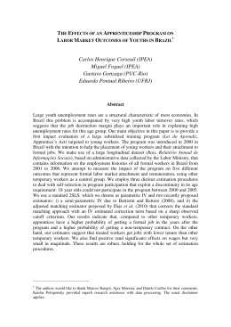
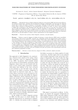
The computing power of a given hardware unit is usually determined by measuring the number of
floating point operations it can perform in a second. Charts on figures 2.1 and 2.2 show the current
measurements of Giga Floating Point Operations per Second (GFLOPS) for single-precision and doubleprecision operations on modern GPUs and CPUs.
From these charts, it is easy to see why GPUs pose such an attraction to programmers needing highperformance applications. A modern high-end GPU can handle around 10 times the GFLOPS of an
equivalent CPU.
However, it is to be noted that these numbers are provided by the GPU vendors. In practice, achieving
such high performance values is immensely difficult (they may even never be reached), as many algorithms
are for instance limited by bandwidth and not by the computing power (being limited by bandwidth means
that the memory cannot provide the data as fast as an execution core would process it).
In our work, we have used a Tesla C2050, which is a workstation card designed specifically for graphics
processing and computing applications (so it is not necessarily suited for video games, which need very
good performance on graphics rendering). Its architecture is further described in Section 2.2.
2.1
Comparing CPUs and GPUs
As seen in the charts in figures 2.1 and 2.2, GPUs are faster on some performance metrics than
CPUs. A few years ago, CPUs increased their performance by increasing their core frequency. However,
increasing the frequency is limited by some physical restrictions such as heat and power consumption.
Nowadays, CPUs’ performance is increased by adding more cores. On computing hardware, the focus is
slowly shifting from CPUs that are optimized to minimize latency towards GPUs that are optimized to
3
Figure 2.1: Comparison of single precision performance between modern CPUs and GPUs.
http://www.feko.info/about-us/News/gpu single precision performance
Figure 2.2: Comparison of double precision performance between modern CPUs and GPUs.
http://www.feko.info/about-us/News/gpu double precision performance
4
augment the total throughput. CPUs that are optimized towards latency use the Multiple Instruction
Multiple Data (MIMD) model, meaning that each of its cores works independently from the others,
executing instructions for several processes.
GPUs on the other hand use a Single Instruction Multiple Data (SIMD) model, where each multiple
processing elements execute the same instruction on multiple data simultaneously.
2.1.1
SIMD Model
The SIMD (Single Instruction Multiple Data) model is suited to the notion that the computation
stages on a GPU are executed sequentially (as in a pipeline) on a flow of data. Each of the computation
stages however, is executed in parallel by the GPU’s processors. In an NVIDIA GPU, processors execute
groups of 32 threads, called warps [5]. Individual threads in the same warp start together, but can then
execute and branch independently (although with some restrictions).
Although threads can generally execute independent instructions, threads belonging to the same warp
can only execute one common instruction at a time. If any thread in a warp diverges, then the threads in
that warp are serially executed for each of the independent instructions, with barriers being inserted after
the execution of such instructions so that threads are then re-synchronized. Thus, efficiency is achieved
when all 32 threads of a warp share the same execution path.
This kind of divergence that forces hardware to serially execute instructions can only exist inside a
warp, as different warps are running on different multiprocessors.
In order to maximize the utilization of a GPU’s resources, thread-level parallelism is needed. Occupancy (the level of threads that are running or ready to run in regards of the total number of possible
threads during the program’s life cycle) is related to the number of warps that belong to a multiprocessor.
Each time an instruction needs to be issued on a multiprocessor, a warp scheduler takes a warp that
is ready to run its next instruction and issues that instruction to the warp’s threads. Some time is needed
for a warp to be ready to execute its next instruction: this is called latency. So thread-level parallelism
effectively targets hiding the latency, and occupancy is essentially a measure of how much latency is
hidden. Maximum occupancy is achieved when the warp scheduler always has an instruction to issue for
some warp at every clock cycle.
2.1.2
Threads
Another main difference between CPUs and GPUs are threads and how they are organized. On a
typical CPU, a small number of threads can run concurrently on a core. On a GPU however, thousands can run concurrently per multiprocessor (our Tesla C2050 card supports up to 1536 threads per
multiprocessor).
Switching between threads on a CPU can also take some significant time, where on a GPU this
switching is done seamlessly and almost instantly. This is due to the fact that on a CPU, the operation
system controls the thread switching behavior. On a GPU, thousands of threads are put into a queue
(in groups of warps). If the hardware must wait on one warp of threads (because for instance it needed
to perform a slow access to memory), then it just swaps that warp with another one that is ready to
execute.
This is mainly possible due to the large amount of registers present on a GPU: separate registers
are allocated to all of the threads, so no swapping of registers or state needs to be done when thread
switching occurs (unlike a CPU, which has less registers and as such their state must be saved in thread
switches).
5
Figure 2.3: The fermi architecture. http://files.tested.com/uploads/0/5/16360-gf100 core.jpg
2.1.3
Memory
Both CPU and GPU have dedicated memory chips available to them. On a CPU, the RAM is
accessible to all code (given that it stays within some boundaries related to processes, boundaries enforced
by the operating system). On a GPU, the RAM is divided virtually (and physically) into several types
(described later in this chapter), each of which has its own characteristics. But mainly the differences are
that the CPU’s RAM is much faster than the GPU’s. The CPU’s RAM has a higher-bandwidth, and it
is supported by multiple, large caches. A GPU’s RAM can be slow depending on the access pattern and
its caches are small, due to being designed for special uses (namely texture filtering) which are related to
the aforementioned types in which the RAM is divided in.
2.2
Hardware Architecture
The Tesla C2050 is an NVIDIA workstation GPU which is based on the Fermi architecture. The Fermi
architecture provides many improvements over previous ones, such as Error-Correcting Code (ECC) across
all of memory types (registers, DRAM, etc) and the ability to execute concurrent processes. The C2050
is composed of 14 shared multiprocessors. A shared multiprocessor is basically a small processor: it has
an execution engine, and plenty of registers. It also has its own small memory and L1 cache. These
14 multiprocessors are then connected to a DRAM memory. In the C2050, this memory has 3GB of
capacity (reduced to around 2.7GB when memory error correction is on). However, its latency is quite
large, so accessing it must be something that programmers must take into consideration when designing
and implementing programs.
In Figure 2.3, we can see an overall look of the architecture present in Fermi GPUs.
6
Figure
2.4:
The
fermi
shared
multiprocessor
http://www.geeks3d.com/public/jegx/201001/fermi gt100 sm.jpg
hardware
architecture.
A Fermi card can have up to 16 shared multiprocessors (our Tesla card has 14), each of which has
capability for 32 cores (or execution units), meaning that at most, 16 x 32 (512) threads can be running
in parallel. They are all inter-connected to a global L2 cache and to memory controllers that are used to
access the GPU’s DRAM. There is also a host interface to communicate with the CPU, and some other
special engines related to graphics operations.
A shared multiprocessor’s architecture is shown in Figure 2.4.
There is a large register file, that is shared between all of the multiprocessor’s active threads. A
multiprocessor also contains a small, fast memory (called the shared memory), and an L1 cache for the
global memory. There is also a special cache, the texture cache. This cache is essentially another cache
for the global memory, but it is optimized for spatial locality and can be populated independently from
the L1 cache.
When it comes to memory, an NVIDIA GPU has different types of physical memory, which can also
be virtually abstracted.There are three main memories on a GPU: device memory, shared memory, and
registers. Device memory is the largest memory (3GB in our Tesla GPU), but also the one with the
largest access latency. It is equivalent to the DRAM of a CPU. Despite being slow, its main use comes
from the fact that it is the only physical memory on the GPU that can be populated by the CPU before
a kernel is launched.
Shared memory is a fast memory that is present on every multiprocessor, and it is shared by all of
7
that multiprocessor’s threads. Its speed comes from the fact that it is present on-chip rather than off
(in other words, shared memory does not need a special bus to be accessed, unlike global memory): no
special buses need to be used to access it. Uncached shared memory latency can be up to 100 times lower
than the global memory’s latency (as long as there are no conflicts in the thread accesses). In order to
achieve such low latency, shared memory is divided into banks. Any memory read or write access made
of some number of memory addresses that are in their own distinct memory banks can therefore be done
simultaneously, effectively increasing the bandwidth. However, if different threads need to access a same
bank, then conflicts arise and accesses need to be serialized (not a big issue as it remains on-chip).
Registers are present on a file in each shared multiprocessor. Every thread has its own set of registers
allocated to it, and register accesses are immediate. Some delays may occur due to read-after-write
dependencies (when an instruction’s operands are not available yet because previous instructions still
need to write them) or bank conflicts, but usually accesses are the fastest that they can be on a GPU.
As for the virtual abstractions, they are all related to the device memory:
• Global memory - Global memory is quite slow, but it can be accessed by 32, 64 or 128 byte transactions. These transactions need to be aligned though: only the first 32, 64 or 128 byte segments
of the global memory that are aligned to their size can be read or written by memory transactions.
When a given warp executes an instruction that accesses global memory, it coalesces the memory
accesses of the threads within the warp into one or more memory transactions, depending on the
size of the word accessed and the requested memory addresses. If requested memory addresses
are far from each other, the warp must effectively perform a single transaction for each memory
address, which causes them to be serialized (and unused words to be transferred). If they however
are completely sequential, then a single transaction can usually be done for all of the addresses: the
hardware performs that transaction and then broadcasts the values to the requesting threads. In a
worst-case scenario with a small number of threads and a very random access pattern, the bottleneck of the execution becomes the global memory: threads are continuously waiting for others to
finish their memory accesses so that they can perform their own.
• Local memory - Local memory space has the same latency and bandwidth as global memory due to
being in the same physical memory. However, this type of memory is organized in such a way that
consecutive 32 bit words are accessed by consecutive threads, and in this way the accesses become
fully coalesced. Local memory, unlike global memory, can not be populated by the CPU or even
the programmer: (large) variables are automatically placed into it by the compiler in the case that
they do not fit into registers.
• Constant memory - This memory space, although residing in device memory, has a small space
allocated to it: 64 KB. But even though it resides on device memory, it is cached on-chip. This
means that a read from constant memory is equal to a read from the cache (which is much faster
than a global memory read). In fact, if threads in a half-warp (which is a group of 16 threads that is
running alongside another one - thus composing a group of 32, a warp - in a shared multiprocessor)
read the same address, that read can be as fast as a read from a register. Reading from different
addresses by threads in a half-warp however, is serialized. Also, this memory is read-only, unlike
global memory.
• Texture memory - The texture memory has basically the same properties as the constant memory,
except that its size is not bound to a fixed value, but the values are that placed into it must respect
some boundaries. It is also optimized for 2-dimensional spatial locality, and it has a dedicated cache.
So threads that read texture addresses close together will achieve good performance. While also
8
read-only, texture memory can be greatly advantageous for algorithms that exhibit spatial locality
in their access patterns.
2.3
Programming Interfaces and CUDA
Developers that want to program GPUs have a choice to make: which application programming
interface to use. The most used ones are:
• Compute Unified Device Architecture (CUDA)[4] - CUDA is a parallel computing architecture
developed by NVIDIA to be used in their GPUs. It provides both a low level and a high level
API, and is composed of simple language extensions for C, as to provide a smaller entry barrier to
developers already used to C or C++. CUDA is also scalable, meaning that it can be seamlessly
applied to NVIDIA GPUs with different characteristics.
• Stream[1] - This architecture is AMD’s response to CUDA. It uses the ”Brook” language, which
is a variant of C designed for parallel computing. CUDA can only be used in NVIDIA cards, and
likewise, Stream can only be used in AMD cards. Stream entered the market later than CUDA, so
its community and environment are significantly smaller than CUDA’s.
• Open Computing Language (OpenCL)[6] - As both CUDA and Stream are proprietary, an open
standard was launched for parallel programming: OpenCL. It can not only be used for GPUs, but
also on every other parallel computing device, be it either a CPU in a server or in a mobile device.
OpenCL is fairly new though, so it is not nearly as mature as the alternatives (especially CUDA).
As we are working with an NVIDIA GPU, our decision of API to use was between CUDA and OpenCL.
CUDA was an easy choice: its developer environment and community were (and still are) much more
mature than OpenCL’s. As programming for GPUs is still relatively recent, challenges related to it are
natural to occur to new programmers , so having an environment with as much support as possible was
important. Also, CUDA provides some much needed performance tools such as a profiler which gives
various data such as occupancy analysis, which helps with getting the maximum performance out of the
GPU.
2.3.1
CUDA Model
The main idea behind CUDA’s model is that it provides abstractions that exist to guide the programmer to partition the problem into sub-problems that can be solved independently by blocks of threads
(which will then be executed on a shared multiprocessor) and each sub-problem into smaller ones, each
of which will be solved by a different thread in a thread block.
Threads and thread blocks are however software entities, while shared multiprocessors are pieces of
actual hardware. Here are the software entities and how they map to the hardware (also shown in Figure
2.5).
• Device - The device is the GPU card that is running the code.
• Host - The host is the CPU that controls the GPU and might also run some code.
• Kernel - A kernel is a function that runs on the device. As mentioned earlier, NVIDIA’s GPUs use
the Single Instruction Multiple Data model. This means that the kernel is executed in parallel by
every thread processor. Recent GPUs have the ability to run multiple kernels concurrently.
9
• Thread and Thread Processor - A thread runs a kernel which is executed on the thread processor
(or CUDA core).
• Thread block and Multiprocessor - Every thread block contains some predefined number of threads.
A multiprocessor executes some thread blocks allocated to it by the GPU, but effectively no more
than a warp of threads (32 threads) can be running on a multiprocessor at a single time.
• Grid - A grid is a set of thread blocks, and a kernel is launched with a given number (specified by
the programmer) of blocks to be run on the device.
Figure
2.5:
Mapping
of
CUDA’s
software
abstractions
http://www.sciencedirect.com/science/article/pii/S1384107609001432#gr1
to
hardware.
By allowing the programmer to specify the number of thread blocks at compile time, programs can
transparently scale to different NVIDIA GPUs with different hardware configurations. The hardware
schedules thread blocks on any shared multiprocessor as long as they are free. However, having the
hardware doing the scheduling also means that we do not have any guarantee if a given thread block has
finished, is executing, or has not begun executing yet.
A kernel’s configuration is an important aspect to consider, as it has an impact on the execution
performance. When a multiprocessor is given one or more thread blocks to execute, it partitions them
into warps that in turn get scheduled for execution by a warp scheduler. A block can have a size up to
a given limit (which depends on the device), but some values are more optimal than others. If a block
has 33 threads, what will happen is that two warps will be created from that block: one with 32 threads,
and one with 1 thread (there are 32 CUDA cores in a shared multiprocessor, thus the scheduler always
builds warps with 32 threads when possible). This will lead to some inefficiency, as at one time only a
single thread will be scheduled for a shared multiprocessor. Blocks should therefore optimally have a size
that is a multiple of 32.
2.3.2
CUDA Workflow
In order to execute a given algorithm in a GPU using CUDA, some steps need to be performed by
the programmer. An example workflow for an algorithm that is to run on the GPU is described:
• First, the programmer implements the algorithm using CUDA’s libraries and C extensions. A kernel
must be defined in order for some work to be performed by the GPU.
10
• The program is then compiled by the CUDA compiler, which translates it into both CPU and GPU
instructions.
• The executable generated in the above step is run.
• Data is read or generated by the CPU and sent to the GPU. The kernel defined in the first step is
then called, which leads to its instructions being sent to the GPU, so it can start executing them.
• The GPU runs the kernel, performing some operations on the data sent by the CPU. When it is
done, the CPU then reads the results back to its memory.
This is a sketch, but it provides a backbone for GPU applications. Even though a small number of
steps is performed, we can see that running a program on a GPU is not as simple as running it on a
CPU: data needs to be sent and read back, which is not an instantaneous process.
2.4
Reflections
As we have seen during this chapter, GPUs have characteristics that set them apart from CPUs:
various memory abstractions, number of cores, differences in threads, etc.
But blindly applying an algorithm to a GPU does not lead to an increase in performance. If for instance
the algorithm needs constant transfers of memory from the CPU, then the performance improvement of
running it in the GPU might be offset by the cost of performing those memory transfers.
The algorithm itself needs to be analyzed as well: if it has highly divergent execution flows between
threads, then the CPU might be a better fit to process it.
GPUs can provide great performance improvements, but some effort is needed in order for them to
do so.
In the following chapter, we will see some examples of pattern matching algorithms which were adapted
to run on GPUs.
11
Chapter 3
Related Work
In this chapter, we present some related work done in the area: standard pattern matching algorithms,
improvements performed on them, and implementing them on GPUs.
3.1
Threat Detection
Threat detection products can be found on a multitude of systems, from personal computers to servers.
Most of them are commercial and require a paid license, having patent-protected algorithms and signature
sets.
SNORT [8] is a widely accepted open-source Intrusion Detection System (IDS). Intrusion detection
systems are a category of thread detection systems designed to scan incoming network packets, as to
detect if an intrusion attempt is underway.
ClamAV [3] is an open-source anti-virus product. Anti-virus solutions scan files instead of packets,
but they also target the detection of possible intrusion or attacks, which might occur if a malicious file
is executed. In order to detect malicious files, anti-virus products employ a plethora of techniques, from
matching a file’s body to a signature set corresponding to known virus footprints, to analyzing their
behavior in run-time.
The fact that they are open-source, together with the support they receive from their parent company
(SourceFire [9]) and their widespread use in the industry, makes them candidate systems adopted for
research in the area.
3.1.1
SNORT
As just mentioned, SNORT is an IDS. Intrusion detection systems work by applying deep packet
inspection techniques to incoming network packets, in order to detect if an attack is being executed.
These deep packet inspection techniques are basically verifying if a given packet matches a signature
from a signature set (taking into account other data such as the protocol that the packet belongs to, for
instance).
Due to being an intrusion detection system, SNORT’s signature set differs from ones from anti-virus
products. While the latter ones are typically just a string (with wildcards or not) that must be matched
on a file, SNORT’s are a little more complex. Also SNORT contains less rules than anti-virus solutions,
but they are a little more complex, as they contain more elements to process.
Each of SNORT’s rules contains an action (or alert), a protocol, a source netmask and port, a
destination netmask and port, and some other options. Of these options, the one named content states
a string that must be matched on the packet. This string, just like regular anti-virus signatures, may
13
alert tcp !$HOME_NET any -> \HOME_NET 80
(msg:"IDS219 - WEB-CGI-Perl access attempt"; flags:PA; content:"perl.exe"; nocase;)
Figure 3.1: Example SNORT rule.
contain wildcards. In contrast, anti-virus signatures usually only contain this string, along with optionally
some other fields such as the offset that the signature must be present in, and the file type in which the
signature must be matched.
There are two main operations needed to be done on each packet to be scanned: packet classification,
and string matching on the packet’s content. According to Roesch [25], the string matching process is
the most computationally expensive one. Thus it is not surprising that research work done with SNORT
typically focuses on improving the performance of this process.
SNORT mainly uses the Aho-Corasick algorithm (described later in this chapter) for pattern matching
purposes. SNORT’s configuration does permit changing the algorithm’s characteristics (such as the type
of the automaton used), but the possible changes in performance due to such different configurations are
not very significant.
Work in the area (also described later on) thus tries to improve SNORT’s pattern matching process,
either by improving the Aho-Corasick algorithm itself, or implementing a new pattern matching algorithm
for SNORT.
3.1.2
ClamAV
ClamAV is an open-source anti-virus engine, used by many people in desktop computers, servers and
mail gateways alike. The signature set of ClamAV contains about one million signatures in total. However, they are not all of the same format. The set is divided in various types, being the most prominent
MD5 hashes and static strings. As of April 2012, the distribution of the signature types was as indicated
by Table 3.1 (the “others” category refers to combinations of signatures, signatures related to archives,
signatures related to spam e-mails, etc).
MD5 Hashes
Basic Strings
Regular
Expressions
Others
Total
1,215,718
88,391
9,421
7,484
1,321,014
Table 3.1: Distribution of signature types in ClamAV.
As we can see, more than 90% of the signatures are MD5 hashes of files. However, MD5 hashes are
calculated by simply applying a hash function to a whole file. Scanning against this type of signatures
does not take a significant amount of time, in contrast to scanning for regular expressions and basic
strings, which must be scanned for inside the file.
This is proven by profiling ClamAV: we did so by scanning a large file (around 600 MBytes), and
found that two functions stood out from the others (considering their execution time). The results are
shown in Table 3.2.
All of the other functions that are not shown in the table had an execution time below 2 seconds
(except for a function related to the database, that took 13 seconds to execute). As such, the biggest
fraction of the running time that we can optimize is the one related to the two functions shown above.
These two functions shown in the table are related to the process of pattern matching, which is done by
14
execution time in
seconds
number of times
called
percentage of
execution time
function name
37.16
2592
38.5%
cli ac scanbuff
36.68
2566
38%
cli bm scanbuff
Table 3.2: Results of profiling ClamAV by scanning a large file.
an anti-virus product in order to determine if a given file contains a known signature (which corresponds
to a virus). As can be seen by their name, are related to ClamAV’s two pattern matching algorithms,
Aho-Corasick and Wu-Manber (the function is actually named “bm”, short for Boyer-Moore; Wu-Manber
is a multi-pattern matching adaptation of Boyer-Moore) - these algorithms will be explained further in
this chapter.
As mentioned, ClamAV’s signature set is quite diverse, but some subset of it needs processing that
is computationally expensive. These signatures can have two different formats (the first of which can no
longer be used to describe new signatures - but old signatures described in it are still valid):
MalwareName=HexSignature
MalwareName:TargetType:Offset:HexSignature[:MinFL:[MaxFL]]
TargetType represents the filetype associated with this signature, Offset represents the location inside a
file where this signature must be present, and MinFL and MaxFL can be used to state that this signature
should be restricted to some detection engine versions.
While the TargetType and Offset parameters represent some computation needed to be done, that
computation is actually only performed if a file matches the hex signature. And it is in this hex signature
that the main complexity of the pattern matching processing lies.
Hex signatures can be split into two different groups: signatures with wildcards, and signatures
without them. Signatures without wildcards are not especially problematic: despite being fairly large
both in number as in length, these can be applied to pattern matching algorithms which don’t have to
worry about matching regular expressions (such algorithms take advantage of that fact to have better
overall runtime complexity). Signatures with wildcards however, can be very problematic: ClamAV’s
wildcards are some of the most complex regular expression characters. Here are some of them:
• ?? - Match any byte. This is equivalent to the “dot” wildcard in POSIX [7] regular expressions.
• * - Match any number of bytes. This is an especially problematic wildcard, as it is equivalent to
the “dot-star” (or “.*”)wildcard conjunction in POSIX. As any number of bytes, and all possible
bytes can be matched here, the regular expression automaton needs to constantly keep considering
the state in which this wildcard is represented.
• {n}, {-n}, {n-}, {n-m} - These are all combinations of repetitions of the ?? wildcard (in fact, {1}
translates to ?? in ClamAV’s internals). While not as problematic as the above wildcard, these
also bring complexity to an equivalent automaton.
Due to the complexity of modern viruses, these wildcards are wildly used in signature sets. In the
ClamAV signature set used (the same as mentioned above), we have found 5,779 “*” wildcards. So not
only are such wildcards highly complex in terms of automaton representation (leading to being expensive
in terms of memory space utilized), but they also exist in a high number. This leads to automata-based
solutions having problems with ClamAV’s signature set, as will be evidenced further along this work.
15
3.2
Pattern Matching
We have already seen earlier in this chapter that pattern matching is the most computationally
intensive task of ClamAV. This is mostly due to the fact that most of the time, every byte of every file (or
packet, in intrusion detection systems) needs to be processed as part of the string searching algorithm.
Pattern matching is the process of finding a string or a set of strings inside a text. Pattern matching
is used widely in variously different applications, from search engines to security solutions.
In order to match a given string ABAB on a text ACABABACAC, we could start by aligning both
of the strings on their first character, and then perform character-by-character comparisons.
Figure 3.2: An example of performing naive string matching.
However, if for instance the text is very long, or if we want to perform matching of several strings
(thus leading to performing the above process for each of the strings), then such a simple process is not
suitable.
For the rest of this work, we will use ClamAV’s notation for wildcards: when a “*” is shown, it is
equivalent to the “.*” wildcard in the POSIX notation regularly used in the industry.
3.2.1
Single-pattern Matching
Single-pattern matching algorithms perform matching of one pattern at a single time. For k patterns
to be matched, the algorithm must be repeated k times.
There are two common single-pattern matching algorithms: Knuth-Morris-Pratt [18] and Boyer-Moore
[12]. Both have a similar backbone idea: that unneeded character comparisons can be skipped by making
use of the information about previously matched characters.
In the Boyer-Moore algorithm, the larger the pattern to search for, the faster the algorithm can match
it. The algorithm compares the pattern to the text from right to left (starting at the rightmost character),
and two rules are used in order to determine how much characters can be skipped when a mismatch occurs
(one is based on the current mismatched character, the other on the number of matched characters before
the mismatch). These rules are dependent on the pattern however, so on each mismatch that occurs, the
distance to be skipped might not be as big as one would hope.
Boyer-Moore can be quite efficient: when the pattern to be searched for does not appear in the text,
its worst-case running time is of O(n + m) (where n is the text length and m is the pattern length).
This is due to the fact that if the pattern does not appear in the text, the algorithm is constantly
skipping characters, without verifying if some possible match exists. When the pattern appears in the
text however, the worst-case running time complexity is O(nm): the algorithm needs to verify possible
matches, and this verification causes the complexity to increase.
3.2.2
Multiple-pattern Matching
Multiple-pattern matching algorithms, in contrast to single-pattern ones, can perform matching of a
set of patterns in a single run. For k patterns to be matched, the algorithm only runs once.
16
Wu-Manber
The Wu-Manber algorithm [33] is very similar to Boyer-Moore, but it can be applied in multiplepattern matching. The main difference is that instead of comparing characters one by one, the algorithm
compares blocks of B characters. In order to do so, it uses three tables: one is analogous to one of
Boyer-Moore’s rules - it is used to determine how many characters in the text can be skipped - and the
other two are used when no shifting, even by a single character, is possible - thus we need to verify which
pattern might be matching at the current position.
A limit m (the length of the smallest pattern) is imposed to the length of each pattern, so that they
all have the same length. A pitfall of this limitation is that if we have small patterns, we can never shift
by a distance greater than the length of the smallest one.
Each possible string in the alphabet is mapped (using a hash function) to an index to the table
that determines the skipping distance (called Shift table). In the scanning phase, there are two possible
situations: either the current string of size B is not a substring of any given pattern (so we can safely
shift m-B+1 characters), or it is. In this latter case, the rightmost occurrence of the string must be found
for all of the patterns, and the shifting distance is then given by the minimum pattern length minus the
greatest of these rightmost occurrences.
As for the other two tables, they are called Hash and Prefix. The Hash table uses the same hash
function as the Shift table, and it maps the last B characters of all patterns. Each entry contains a pointer
that both points to a list of pointers to patterns whose last B characters hash into the corresponding
index of the Hash table. The pointer contained in each entry is also in turn an index to the Prefix table.
This Prefix table maps the first B characters of all patterns into a hash value. It is mainly used to filter
patterns whose suffix is the same as the current string that was matched, but whose prefix is different.
Considering this, the scanning procedure is as follows: a hash value is calculated for the current B
text characters. The value of the Shift table for this hash value is then checked: if it is geather than 0,
then the text is shifted by the given value, and the matching resumes. If not, then the hash value of
the prefix of the text (starting m - the minimum pattern length - characters to the left of the current
position) is calculated.
After this, for each pattern that is pointed to by Hash table for the first hash value that was calculated,
we must check if its entry in the Prefix table is equal to the recently calculated hash value of the prefix.
If they are equal, then the pattern is checked directly (character by character) against the text, in order
to confirm the match.
The Shift table is constructed in O(M) time (where M is the total size of the patterns), and one
hash function takes O(B) (B is the block size - a value that can be defined, but recommended by the
algorithm’s authors to be 2 or 3 for natural language texts) to compute. As such, the total amount of
work in the case of non-zero shifts is O(BN/m) (N is the text size, and m the minimum pattern length).
The algorithm is not only designed to concentrate of typical searches (rather than worst-case behavior),
but also it is designed to be used for natural language texts and queries, so it might not be as efficient
on other applications whose pattern sets might have different characteristics than the ones from natural
language. In Chapter 4, we will show that this holds true: not every application benefits (in terms of
execution time) from using the Wu-Manber algorithm.
Burrows-Wheeler Transform
The Burrows-Wheeler-Transform (BWT) is a reversible transformation that can be performed on
a text, in order to achieve compression. It has been widely used in that area, but its application to
string matching was only discovered in 2000 [14]. In order to do string matching with BWT, one must
do pre-processing on the text (in contrast to other algorithms such as automata-based ones, which do
17
pre-processing on the queries).
The BWT for a given text T is constructed by first appending an “end of string” character (the $
character for instance) to the text (this character should of course not be present in any other position in
the text). Then, all of the cyclic permutations of the text are calculated and sorted. The BWT is then
given by the last character of each of the cyclic permutations, which are arranged in sorted order.
Two additional data structures must also be present: an array, which keeps track of the original
indexes of the permutations before being sorted (called the suffix array), and another one which keeps
the sorted characters of the string.
Searching is done as follows: for each character in the query, we find the corresponding cyclic permutations of the text whose first characters are equal to the one being considered from the query. We
continue on to consider the next character query: we again find its corresponding permutations, but
this time we only consider the first n permutations, where n is the number of times that this character
appeared in the set of last characters from the previously considered cyclic permutations. When we have
done this for all of the characters of the query, the indexes of where the query is present in the text are
given by the suffix array values corresponding to the cyclic permutations who where considered last.
While searching is done in a straightforward manner, BWT-based pattern matching algorithms have
as can be seen, a quite large memory usage: different data structures must be kept in memory, and these
can grow to be quite large depending on the text (around 3.7GB for the human genome [20]). Also,
BWT is more suited for applications which have a fixed text and changing queries (as it applies the
pre-processing on the text).
Finite automata
Other multi-pattern matching algorithms are based on finite automata. Finite automata used in
pattern matching algorithms are either non-deterministic (NFA) or deterministic (DFA). Both kinds are
augmented: directed graphs that have an alphabet, a set of states, and a transition function (that for
each sate, computes a next state, given a character from the alphabet).
Matching is done by, starting at the initial state, computing the value of the transition function for
the current input character, and feed that value to be the next state at the next iteration (where the
transition function is again executed but for the next input character). When one of the states given
by the transition function is final, the algorithm reports that there was a match at the current input
position.
Non-deterministic Finite Automata
A Non-deterministic Finite Automaton (NFA) consists of a finite set of states Q, a finite set of input
symbols Σ called the alphabet, a transition relation ∆ : Q × (Σ ∪ {}) → P (Q) (where P (Q) represents
the set of all the subsets of Q and represents the empty string), a start state q0 ∈ Q and a set of final
states F ⊆ Q. Let a = a1 , a2 , ..., an be an input string over Σ. The NFA recognizes a if in Q a sequence
of states s = s1 , s2 , ..., sn respects the conditions
• s0 ∈ E(q0 ) (the automaton starts in the states reachable by transitions from q0 )
• s0 ∈ ∆(si , ai+1 ) and si+1 ∈ E(s0 ), (i = 0, 1, ..., n − 1) (the next state to transition to is given by
the result of applying the transition relation with the current state and input character, and then
following transitions for the resulting state)
• sn ∈ F (the automaton recognises the input string of any of the states to which it transitions to is
part of the set of final states)
18
Figure 3.3: NFA for the patterns ab*c, c and ad built from applying Thompson’s algorithm. [29]
The execution model of an NFA uses some auxiliary data when processing the input text. As in an
NFA the system may be at more than one state at a single time, usually a vector is kept, which represents
a list of active states. Each time one of the active states is final, the algorithm reports a match for the
possible final states.
An example NFA for the patterns “ab*c”, “bc” and “ad” (where ”*” is the ClamAV wildcard, representing the possibility of zero or more characters being matched) is shown in Figure 3.3. A transition
labeled by Σ represents a group of transitions for all of the characters in the alphabet, which in this case
is Σ = {a, b, c, d}.
Matching on an NFA is a somewhat different (and more complex) process than matching on a DFA:
instead of only following a single transition on each input character, multiple transitions are followed,
which leads to several states being active at any one time.
The process of matching the NFA from Figure 3.3 to the text abc is:
• The only active state at the start of the algorithm is the initial state, state 0.
• On consuming the first character, a, the algorithm marks states 1 and 9 as active.
• The character b is consumed, leading to states 1 and 9 being marked as inactive, and states 2, 3, 5
and 7 marked as active (state 0 is always active, and epsilon transitions are always followed).
• The algorithm finally consumes the character c, which leads to the states 6 and 8 being marked as
active (and states 5 and 7 as inactive). These states are final, so matches are reported on each of
them.
Deterministic Finite Automata
A Deterministic Finite Automaton (DFA) consists of a finite set of states Q, a finite set of input
symbols Σ called the alphabet, a transition function δ : Q × Σ → Q, a start state q0 ∈ Q and a set of final
states F ⊆ Q. Let a = a1 , a2 , ..., an be an input string over Σ. The DFA recognizes a if in Q a sequence
of states s = s1 , s2 , ..., sn respects the conditions
• s0 = q0 (the automaton starts in the state q0 )
• si+1 = δ(si , ai+1 ) (i = 0, 1, ..., n−1) (the next state to transition to is given by the result of applying
the transition function with the current state and input character)
19
a
b
c
d
0
1
2
0
0
1
0
3
0
4
2
0
0
5
0
3
3
3
6
3
4
0
0
0
0
5
0
0
0
0
6
3
3
6
3
Table 3.3: Transition table for the DFA in Figure 3.4
• sn ∈ F (the automaton recognises the input string of any of the states to which it transitions to is
part of the set of final states)
The transition function δ can be represented in different ways, but the standard one is using a 2dimensional table. Each of the table’s cells includes the result of applying the transition function to the
state and input character given by the respective line and column. As an example, for the DFA in Figure
3.4, we can represent its transition function using Table 3.3. All of the cells in the first row represent the
transitions that will occur at state 0 for each of the input characters. Conversely, the cells in the first
column represent the transitions for the input character ‘a’ that will occur at every state. We can see
that the cell given by the first row and first column has the value 1. This means that if the automaton
is on state 0 and the input character is an ‘a’, then the automaton transitions to state 1.
Comparing DFAs with NFAs, a DFA has no transitions by the epsilon character and each state only
has one transition by a given character. This simple model has two main advantages: first, matching
is straightforward and fast, as it requires only a single table lookup (or pointer dereference) per input
character. Second, DFAs are composable, meaning that a set of DFAs can be composed into a single
composite DFA (eliminating the need to transverse multiple DFAs instead of a single one).
Unfortunately, DFAs often do not interact well when combined, yielding a composite DFA whose size
may be exponential in input and often exceeds available memory.
They do however provide a big advantage over NFAs: as computers are deterministic machines, NFAs
are harder to simulate in them (due to the possibility of being in more than one state at the same time),
which causes larger execution times and greater implementation complexity.
Regular expression matching with automata
Regular expressions are gaining widespread use in applications which use searches with expressive
and flexible queries (virus scanning and intrusion detection are examples of such applications). Using
Thompson’s algorithm [29], an NFA can be converted from a regular expression, and then converted to
an equivalent DFA.
As regular expression use becomes more and more common in packet and file scanning applications,
it is imperative that regular expression matching be as fast as possible, as to keep up with line-speed
packet header processing. The inefficiency in regular expression matching is largely due to the fact that
the current matching solutions do not efficiently handle some complex features of regular expressions used
in such applications: many patterns use multiple wildcards (such as ‘.’ and “*”) and some patterns can
contain over ten such wildcards. As regular expressions are converted into NFAs for pattern matching,
large numbers of wildcards can cause the corresponding DFA to grow exponentially. Also, a majority of
the wildcards are used along with length restrictions (such as ‘?’ and ‘+’), and these restrictions can
20
increase the resource needs for expression matching. Finally, groups of characters are also commonly
used in regular expressions (such as one that matches all lowercase characters). Groups of characters can
intersect with one another or with wildcards, causing a highly complex automaton.
Converting an DFA to a DFA
The method to convert an NFA to a DFA is called Subset Construction [24]. Its general idea is that
each state of the DFA corresponds to a set of NFA states. So, when calculating the transition function
for the input, each time the DFA is on a given state, it is also on a set of NFA states.
The algorithm constructs a transition table for the DFA to be built, which will represent for each
state and input character, what will be the next state to transition to. As we are building a DFA from
an NFA, these DFA states will be represented by sets of NFA states. This transition table is built so
that the resulting DFA will end up simulating all of the possible transitions that the NFA can make in a
given input string.
The algorithm defines some operations which effectively give us the resulting set of states that an
NFA has active after performing a transition. Remembering that the NFA can have transitions by the
empty character, which does not consume input, it is clear to define that the set of NFA states that is
active after a given transition is the state s that is given by that transition, plus all of the states given
by epsilon transitions starting from s.
If we repeatedly consider each of these sets of NFA states for the transition table that we want to
build, we end up with a deterministic automaton that for each set of NFA states N and input character
c, gives us another set of NFA states which is composed of states reachable (either by just following a
transition or by following multiple epsilon transitions) by each of the states in N by transitions labeled
by c.
The result of applying the algorithm for the NFA in Figure 3.3 is shown in Figure 3.4 (consider that
the “*” wildcard is the ClamAV one, the equivalent in POSIX would be “.*”).
The conversion algorithm does have a nuance though: it does not give as an automaton capable of
continuous matching (for the situation in which we want to identify all matching patterns in a text, and
not only a single one).
This in turn affects the online complexity of scanning a text using the resulting DFA: if we reach a
given state and the transition for the current input character leads to the initial state, then we must
backtrack on the input (we must re-consider the failed input text). This causes the complexity of the
algorithm to no longer be O(n) on every case - if we need to backtrack, then we must read the input
character that caused the failure transition again; this of course is not ideal (we want an O(n) scanning
algorithm).
However, a simple modification (in implementation terms) can be made to the subset construction
algorithm to make it build a DFA capable of continuous matching. We just add a new transition by
sigma (all of the input characters) from the initial state to itself. What this entails to, is that at each
point in the DFA transition-table building process, we are always considering transitions from the initial
state, and this will propagate throughout the process: we will end up simulating the NFA not just for its
valid input characters, but for every character in the alphabet.
While this allows the algorithm to provide us with an automaton capable of begin used for continous
scanning, it also greatly increases the conversion algorithm’s complexity (there are now many more possible input characters to consider at every state, instead of just the ones present on the NFA transitions).
The resulting DFA can be extremely more complex as well. Figure 3.5 shows a DFA built from this new
version of the algorithm. We can see that considering all of the input characters greatly increased the
DFA’s complexity, namely at the point representing the wildcard (state 3).
21
Figure 3.4: DFA for the patterns ab*c, bc and ad.
Figure 3.5: Complete DFA for the patterns ab*c, bc and ad.
22
To illustrate the advantage, consider what happens when the input is abad. In the first automaton,
the matching gets stuck on state 3 waiting for a c to come in the input, so no match will be reported,
which is incorrect. In the second automaton, if we just follow the transitions, then we see that a match
for ad is actually reported (on state 12). And if afterwards came a c, then the automaton would also
report a match of the ab*c pattern (this would also happen on the first automaton).
What is happening is, at the state that represents the star wildcard, the automaton actually represents
the possibility of every other pattern in the set being present in the input. If our pattern set contains
many wildcards and many patterns (as is the case in ClamAV as in previous sections), we can see how
this becomes a huge problem.
Some approaches have been proposed to counter the state-space explosion that affects DFAs constructed from regular expressions with complex wildcards: HFA [11], hybrid finite automata, split the
DFA under construction at the point where state-space explosion would happen. Lazy DFAs [15] keep
a subset of the DFA that matches the most common patterns in memory; for uncommon strings, they
extend the subset from the corresponding NFA at runtime. This causes the Lazy DFA to be smaller
than the corresponding complete DFA, while providing good performance for common patterns. However, a malicious sender can input widely different patterns into the system, causing it to be dynamically
rebuilding a DFA (and thus slowing down the overall system).
Smith et al. [26] proposed another alternative called XFA, which uses less overall memory than DFA
but requires, for each state, some auxiliary memory (used to track the matching progress) along with
computation. In order to reduce a DFAs memory footprint, they apply the idea that on each state,
instead of having for instance two separate transitions to two different states, they can be grouped into
a single one, which goes into a single state. This state will then have some computation associated with
it, which will differentiate each of the two states that were grouped into this single one. By doing this,
DFAs are effectively compacted, at the cost of some more computation. While the memory cost is greatly
reduced, per-byte complexity is increased, which is not an ideal tradeoff for all applications.
Aho-Corasick
A special automata-based algorithm is the Aho-Corasick algorithm [10]. It uses a DFA in the form
of a trie, which is a data structure just like a tree, except that it is ordered and it is used to store an
associative array. The DFA used in Aho-Corasick is not the classical one: instead of having transitions
for each character of the alphabet on each state, it has transitions for characters that lead to other states
in the same expression (just like a regular DFA), along with failure transitions. These failure transitions
are followed each time a mismatch occurs, and they are designed to keep track of shared prefixes between
patterns (thus allowing the automaton to transition between matches without backtracking).
Using the Aho-Corasick algorithm for string matching consists of (roughly) two steps, like other
automata-based algorithms: first, a single composite automaton is generated from the patten set; afterwards, that automaton is traversed in order to recognize the corresponding patterns in a text. Given a
current state and an input character, the Aho-Corasick algorithm first checks whether there is a valid
transition on the automaton for the next input character. If there is, then that transition is followed;
otherwise, the failure transition is the one followed and the same input character is considered until it
causes a valid transition. In other words, unlike valid transitions, failure transitions do not cause the
input character to be consumed.
Note that in the latter case, the input character is actually read more than once for different reads of
states from the automaton. This means that Aho-Corasick’s complexity is not O(n) as we would hope.
Aho-Corasick cannot also be used for regular expression matching. ClamAV uses it for scanning files
against signatures with wildcards, but it does not actually represent the wildcards in the automaton
23
(which is what would happen in classical automata based algorithms). It splits the signature into parts
divided by its wildcards, and considers each part as an individual pattern. Then, when two patterns
match, ClamAV inspects what occurred between the matches, and compares that against the wildcard
that separates the matched parts. This causes ClamAV to not have the best efficiency in terms of running
time (as if matches occur then further verification is needed), but it also causes it to have a very low
memory footprint. As it is designed to run on headless servers (namely e-mail gateways) which might
have a very small memory footprint, memory efficiency is a bigger concern to ClamAV than raw scanning
performance.
The main reason that ClamAV uses Aho-Corasick is that many parts in the signatures containing
wildcards are short, and thus considering separate small parts in Boyer-Moore would further restrict the
shifting distance, which is already bound by the length of the smallest signature. As for the usage of
Wu-Manber, compared with the sparse automaton representation used by Aho-Corasick, the shift table
present in Wu-Manber is a more compact representation of a large number of signatures that don’t contain
wild cards, leading to lower memory usage.
We have presented the standard industry pattern matching algorithms. For the rest of this section,
we shall describe related work that focuses on improving them.
3.2.3
A Sub-linear Scanning Complexity Algorithm
Huang et. al [17] proposed a pattern matching algorithm which is sub-linear in the scanning time
complexity. It uses a shift table and hash technique (somewhat similar to Boyer-Moore) and inspects
overlaps between pairs of patterns to ensure worst-case performance. Huang et. al calculated the average
pattern length of ClamAV, and like was shown earlier in this chapter, they found that it was lower than
the one on other systems such as SNORT. It was due to that observation that they decided to use a shift
and hash technique (also ClamAV at the time only had used a shift technique in its algorithm). They also
found that the number of long overlaps between suffixes and prefixes of pattern pairs was limited and as
such, their algorithm can shift more bytes after a pattern is matched, ensuring worst-case performance
(where many patterns are present in the text).
The proposed algorithm consists of two phases: an offline preprocessing phase, where the shift table
is constructed like in the Wu-Manber algorithm. Along with each pattern, a list is also stored, composed
of prefixes of other patterns, that overlap with the suffix of the one they are being associated with. This
allows the algorithm to continuously perform matching on the text, and detect multiple patterns that
overlap with each other.
The other phase of the algorithm is the online matching phase, in which a lookup is performed on the
shift table. If the shift value is zero, the prefix hash is calculated and compared with the value present
in the list. If the hash table entry is empty, then the matching continues starting from the prefix’s last
character. Otherwise, exact comparisons are made for each possible pattern (whose prefix hash is the
same as the one that was just calculated) to confirm a possible match.
If a pattern is matched in this phase, then the algorithm checks its data structures to try to find a
consecutive overlapped pattern (and thus match more than one pattern in a single algorithm iteration).
The proposed algorithm was found to have a speed-up of around 6 and 1.5 for the Aho-Corasick and
Boyer-Moore implementations in ClamAV, respectively, while consuming roughly the same amount of
memory.
3.2.4
Rearranging the Aho-Corasick States
When it comes to the Aho-Corasick algorithm, Nishimura et al. [23] proposed speeding it up by
rearranging its states.
24
The Aho-Corasick algorithm consists of two parts: first, a pattern matching automaton is constructed
from the given pattern set; then that automaton is used to search the text. The time complexities of
both parts of the algorithm are, respectively, linear in the total length of the patterns, and linear in the
length of the text.
The pattern matching machine is usually implemented as a two dimensional array (with O(nm) space
complexity, where n is the number of states and m is the alphabet size), which represents a table that
is inspected at each input byte, in order to fund which transition on the state machine should be taken.
The execution time of searching for the patterns in the text depends on the time that it takes to transmit
data from primary or secondary storage. In order to reduce this overhead, data compression can be
used to reduce the text’s and the patterns’ size, therefore decreasing the table’s size and the primary or
secondary storage transmit time. However, a high compression ratio of the patterns and text does not
necessarily lead to a speedup in the matching phase of the algorithm.
In order to make the frequently used states be collected on RAM in order to improve CPU cache
efficiency, Nishimura et al. proposed rearranging them in a breadth-first order: frequently used states
are usually close to the initial state.
Using the rearranging techniques led to a reduction of about 71% in the matching time on a random
text (on an English natural language text, the reduction was of 80%). Such an improvement was possible
due to the pattern set characteristics, causing mismatches to occur often and early. If that was not the
case, the reduction in matching time would not be so significant.
3.2.5
Re-writing some Regular Expression Rules
We have seen earlier in this chapter that some regular expression rules can be quite problematic for
DFA, leading to state-space explosion. Yu et al. [34] tried to optimize DFAs by re-writing some of these
rules. Remembering the problem of regular expressions, a pattern can be matched on the entire input
string or on specific substrings of the input, rather than being only matched on a simple string (of fixed
length). Without a priori knowledge of the starting and ending positions of those substrings, DFA created
for recognizing all substring matches can be highly complex, and such a feature (reporting all matching
substrings) may not be fully necessary for the application being considered. In fact, in payload scanning
applications (intrusion detection systems and anti-virus solutions) we are only interested in knowing if
certain attacks or patterns are present.
Some regular expressions have a special character to indicate that this expression should be matched
only at the beginning of a line. Without this character, there is no prior knowledge of whether or where
a matching substring may appear. To handle these patterns, two types of DFA can be created: repeated
searches or pre-pending ”.*” to each of these patterns (thus explicitly stating that the pattern can occur
anywhere in the input). As the input is scanned from start to end, the DFA can recognize all substring
matches that may start at different positions of the input.
However, patterns that do start with “∧ ” may also bring some problems. If there is a class of characters
that can overlap with the pattern’s prefix (such as for instance the rule “∧ B+[∧ n]” which means matching
at the beginning of a line a positive number of Bs and then anything except a newline), then the resulting
DFA can be quite complex (because in the given example the DFA needs to remember the number of Bs
it has seen and their locations in order to make a correct decision with the next input character).
From an analysis done by the authors, a significant number of patterns in the SNORT rule fell into
this category. In order to solve this issue, they proposed re-writing such patterns. In the example given
above, due to the fact that in payload scanning applications only non-overlapping matches are of interest,
the pattern could be rewritten to “∧ B[∧ n]”.
For patterns targeting buffer overflow attempts (existing on intrusion detection signature sets), that
25
have a length restriction and check if newlines are not present in the pattern, they proposed adding the
“∧ ” character, avoiding state-space explosion.
They also proposed algorithms to efficiently group patterns together, such that patterns in each group
do not adversely interact with each other. Two patterns interact with each other if their composite DFA
contains more states than the sum of the two individual ones. This can clearly happen in our work, as
plenty of patterns contain a wildcard equivalent to “.*”, and we wish to be able to transition between
states of different patterns (as to guarantee O(n) performance).
In order to perform the grouping, they used the notion that if there is no interaction between any
pair selected from three regular expressions, the composite of those regular expressions is not likely to
exceed the sum of the individual ones. Grouping is done for every pair of regular expressions that do not
interact, and until the group dimension is not exceeded (a threshold that is manually set).
Using these re-writing techniques, the authors found that the overall DFA reduction rate in the SNORT
signature set was of about 98%, a large improvement. When it comes to grouping multiple patterns, they
found that the signatures in another intrusion detection system, Bro [2], could all be grouped, so creating
a composite DFA greatly improved the throughput for this signature set. Their implementation was
overall 48 to 704 faster than an NFA implementation. However, the memory usage was still about 3
to 8 times the one used by an NFA-based approach. Another disadvantage is that rewriting patterns is
something that has to be done specifically for each signature set, and as such cannot be automated.
So while in fact this set of techniques does bring benefits in terms of throughput increase and some
memory reduction, this reduction (which might not be sufficient in every application) comes at a cost of
having to be manually implemented, which may not be feasible for huge signature sets, like for instance
that of ClamAV.
3.2.6
Symbolic Finite State Transducers
One of the biggest security threads in the web is (and has been for some years) Cross-Site Scripting
(or XSS). Cross-Site Scripting is possible due to the existance of a flaw in a server, allowing a client to
send data containing malicious code, that will then in turn be sent to and executed by browsers belonging
to other clients. This flaw is usually present on servers due to the non-escaping of some some critical
characters that are specific to code from web pages. If these characters are not modified in any way when
they are sent to other clients’ browsers, then the browsers will interpret them as valid code instead of
data to be viewed. Writing string manipulating functions to handle these specific characters is a hard
problem, as the functions must be efficient and bug-free.
Veanes et. al [22] addressed this issue by using symbolic finite state transducers (which extend classic
transducers - a special automaton allowing for both input and output data on each state - with symbolic
predicates). The key difference between these symbolic finite state transducers and classic finite state
transducers is that each transition, instead of being labeled by a character, is labeled by a formula.
Therefore, if we are at a given state of the transducer, we can only advance to a next state if the current
character respects the formula for the corresponding transition (usually these formulas are like a range
that the character must be in, or a specific value that the character must have).
By having different possible execution flows at each state, the traversal of the transducer is not trivial
for a processor: on each state, instead of simply following the transition, the formula for each transition
must be checked, and if it is satisfied, then we can proceed its corresponding state.
Chapter 2 showed that divergence is one of the main factors that can cause a great loss of performance
in GPUs. As such, symbolic finite state transducers are not at all appropriate for a GPU, as they have
different execution flows on each state.
So far, we have seen standard improvements done to the standard pattern matching algorithms in-
26
troduced earlier in the chapter. We continue to present work that improves them, but doing so by
implementing them in GPUs.
3.3
Pattern Matching on GPUs
With the rising computational power of GPUs, research has been done for their use in several application areas. Many of such areas require pattern matching algorithms, so implementing them in GPUs
is a key factor in improving the overall performance.
Kouzinopoulos et al. [19] performed a comparison of the execution times of parallel versions of
the Knuth-Morris-Pratt [18], Boyer-Moore Horspool [16] (an improvement over the classic Boyer-Moore
algorithm), and Quick-Search [28] algorithms on an NVIDIA GPU. These algorithms were run on several
bacteria sequences, as genome sequencing is one of the areas that benefits the most from GPUs being
used for pattern matching. They also ran a naive string searching algorithm, and they found that the
speedup compared to the CPU-only version, was of 2.4.
The speedup achieved in Knuth-Morris-Pratt, Boyer-Moore Horspool and Quick-Search was of 18, 20
and 19 (respectively), proving that GPUs can be quite efficient on pattern matching. They found that
the speedup could be further improved by only using the GPU’s shared memory (instead of using the
global memory).
They concluded that the GPU can run string matching algorithms in a very efficient manner, outperforming the CPU. However, in order to do so, these algorithms cannot be directly ported from the CPU
to the GPU: they have to be adapted in some way in order to fully use the GPU’s computational power.
3.3.1
Using SNORT Signatures
Extended Finite Automata on the GPU
Smith et al. [27] implemented a pattern matching system on a GPU based on XFA (introduced earlier
in this chapter). While XFA might seem like a good improvement, they introduce serious challenges for
SIMD architectures. Having more variable updates involve memory accesses in a manner different than
the access patterns used for traversing an automaton. In a GPU memory accesses should be as few and
simple as possible, as they pose one of the most common bottlenecks of an algorithm.
In addition, some XFA use offset counters, which are just like standard counters but store the vale in
an offset list. These special counters, while eliminating some increment instructions, require additional
work at each byte read.
Performing matching with a DFA has two levels of control-flow: a function is applied to every input
string, and then that function iterates every character of the input string. XFA have a third level: for
each state, the interpreter must then execute every instruction for that state and then iterate over the
entries in the offset list (in order to increment the respective counters). It is clear that processing these
instructions causes many conditional branches.
XFA thus suffer from large amounts of control flow divergence in their third level: as a statement
must be evaluated on each state, different instructions may be executed after that evaluation.
In their implementation, the authors found that the percentage of SIMD instructions that diverged was
more than 50%. As mentioned on Chapter 2, modern GPUs do support divergence, but at a (sometimes
large) performance cost.
The authors concluded that signature matching requires memories that support efficient regular accesses, some fast accesses to a smaller memory and capabilities to hide the latency of irregular accesses.
These are all characteristics that are present on modern GPUs, so DFA processing (which has a somewhat
predictable control flow) should be efficiently supported.
27
As their proposed XFA alternative exhibits branching that is dependent on the input data, it cannot
be reasonably supported by GPUs. The authors did propose that as they found such branching infrequent
on real traffic, some mechanism could be implemented to deviate from SIMD instructions once data that
could cause divergence was found.
Measurements from their work proved the disadvantages of XFA: their measured speedup with XFA
was of about 6.7, while a DFA implementation reached 8.6.
They proposed caching the XFA on the GPU in order to improve throughput, but this could also be
done for DFA, so the performance issue should not be tackled from an implementation point-of-view, but
rather from a design one.
Porting of Aho-Corasick to the GPU
Vasiliadis et. al proposed a solution in which the Aho-Corasick algorithm was ported to the GPU, in
order to perform high-speed intrusion detection [30].
Section 3.1.1 described the SNORT intrusion detection system, which organizes the signatures in
groups based on the source and destination port numbers of each rule (it therefore groups signatures
based on the protocol that the packets that contain such signatures use).
In the authors’ implementation, a separate detection engine instance is used to match the patterns
belonging to a rule group. In order to improve the CPU to GPU memory transfer throughput, each rule
group is copied using a buffer that was allocated using page-locked memory. The CPU to GPU transfer is
also performed using direct memory access, thus freeing the CPU during this time. They have also used
a double-buffering scheme, so that when the first buffer becomes full, it is sent to the texture memory so
that the GPU can process it. While this processing is in place, the CPU is copying newly arrived packets
in the second buffer.
The processing that the GPU performs is the execution of the Aho-Corasick algorithm. The automaton
used by Aho-Corasick is stored in a traditional two-dimensional array, where each cell contains not only
the information of the next state to move to, but also information regarding whether that state is final
or not. As to improve memory access efficiency, the automaton is stored in the GPU’s texture memory.
Two different parallelization methods were implemented. In the first one, each packet was split into
parts of an equal (and fixed) size. Each thread then searches each part of the packet in parallel. In the
second method, each thread is assigned a whole packet to search in.
Every time a thread matches a pattern inside a given packet, it reports the occurrence by appending
the pattern to an array present in global memory. The reports for each packet will be written in a
separate row of the array, following the order that they were copied to texture memory. This means that
the array will have the same number of rows as the number of packets contained in the batch, which
can grow to be quite large. This array is also copied to the CPU memory when the pattern matching
execution has finished, as for the CPU to report the occurrences of matched patterns.
However, reporting an occurrence is not a simple task, as some corner cases must be handled. Casesensitive patterns (Aho-Corasick is a case insensitive algorithm) must be handled by performing an extra
search, offset-oriented rules (which state a location on the input string where the pattern must be present)
must be explicitly checked, and patterns with a common suffix must be confirmed.
Returning to their proposed parallelization methods as briefly described above, each of them has its
own advantages and disadvantages. In the approach of assigning parts of a packet to each thread (and
assigning a packet to each multiprocessor), all threads are assigned the same amount of work. This causes
the execution to have very little divergence (which as seen would hinder SIMD execution). Moreover, in
this case the texture cache is used entirely for the state tables, as no other data is present on the texture
memory.
28
A drawback of this approach is that extra processing is needed for solving the border detection
problem. What happens is that as each thread is assigned a different part of each packet, there is a
possibility that some patterns are not found, as they could start in a given part and finish in another one
(so a thread would never completely finish the matching of such a pattern). In order to solve this issue,
all of threads must scan a little longer (the largest pattern’s length) than the length of their assigned
part. The authors mention that, as each packet is copied to the shared memory of each multiprocessor,
communication costs between threads are avoided. But if a packet is so large as it cannot fit into the
shared memory (which in our Tesla C2050 card is 48KB), then these costs are no longer avoided.
As for the second approach, assigning a single packet to each thread, its biggest disadvantage is that
different threads have different amounts of work (due to varying packet sizes). This means that threads
of a same warp will have to wait until all of the threads in that warp have finished searching in the packet
that was assigned to them. However, no additional computation will occur since every packet is processed
in isolation.
The authors found that overall, due to the cost of divergence in the execution, the best parallelization
method was assigning chunks of packets to different threads.
They found that the system’s performance was quite good, as it yielded a speedup of 2.4. The CPU
was not completely offloaded though, so this opens up the system to targeted attacks. An attacker could
craft packets that would need to be able to be verified by the CPU (after the GPU processing), thus
slowing down the system.
Lin et al. [21] also proposed a port of the Aho-Corasick algorithm to the GPU, but with a somewhat
different approach than the one by the work described above. As stated, a problem with running the
Aho-Corasick algorithm on a GPU (while dividing the file(s) to be scanned amongst threads, which
is a direct implementation of the algorithm) is boundary detection. This problem can be resolved by
having threads process overlapped computation on the boundaries, but the overhead of such overlapped
computation can degrade the performance.
Due to this issue, the authors opted for another approach: instead of assigning a packet’s chunk to a
thread, they assign each byte of the input stream in order to identify any pattern that may start at the
thread’s starting location.
This idea of allocating each byte of an input stream to a thread to identify any virus pattern starting at
the thread starting location has an important implication on the efficiency. First, in the conventional AhoCorasick automaton, the failure transitions are used to back-track the state machine when a mismatch
occurs, so as to identify the patterns starting at any location of an input stream. Since in the proposed
algorithm a GPU thread only needs to check for patterns starting at a particular location, back-tracking
is not needed. Therefore, the failure transitions of the Aho-Corasick automaton can all be removed. And
also, as each thread is allocated a different input stream byte to search for, there is no need for border
detection.
The authors’ algorithm allocates a large number of threads, and most of these have a high probability
of terminating early. This means that threads will have to wait for others in order to proceed, which can
lead to some overall performance loss.
In the implemention, the authors used the maximum number of threads per thread block. The AhoCorasick automaton was split as to be able to fit into each multiprocessor’s shared memory. The split
was done by dividing all of the patterns into several groups (patterns of a same group have some prefix
similarity), and separately compiling these groups into smaller state machines, leading to lower memory
usage. Due to the fact that all threads of a warp traverse the same state machine (which has no failure
transitions) but start at different bytes on the input stream, it is likely that many threads terminate much
earlier than others. In order to fully utilize the stream processors of the GPU, the authors evaluated
two different ways to assign the threads. A first approach was to equally distribute the bytes of an input
29
stream to each thread of the same block. A second one was to utilize a global variable that assigned new
jobs to threads that have already finished. As this variable can only be accessed by a single thread at
a time, its accesses should be atomic. Atomic accesses in a GPU can lead to a serious degradation in
performance, as threads need to wait for the same resource. The authors decided, based on experimental
results, that equally distributing the bytes of an input stream to each thread was the right approach to
use.
Their results found that the system had an overall 2 to 2.5 speedup over the CPU version (taking into
account memory transfers). Although a nice improvement in performance, the authors’ proposed system
has a simplistic work division, leading to possible uneven work between threads (depending on the input
data).
Regular expression matching
Vasiliadis et al. [32] extended SNORT to support regular expression matching using a GPU. The
proposed system is based on DFA: all of the contained regular expressions of the SNORT signature set are
compiled and converted into DFA using Thompson’s algorithm. Unlike regular DFA-based solutions, in
the proposed work, each regular expression is compiled into a separate automaton (that is then transferred
to the GPU). This work effectively serves as an extension of one described above by the same authors,
but which performed regular expression matching on the CPU. In this one, packets are sent to the GPU
along with an identifier of the regular expression that they need to be matched against. So packets are
not scanned in parallel on the same automaton, but on different ones.
During the search phase, all of the automata reside in the GPU’s texture memory. Using the identifier
of the regular expression, each thread will scan the whole packet in isolation.
The automata used do not support all possible wildcards of a regular expression though (in order
to prevent state-space explosion). So in order to preserve accuracy and precision, all of the regular
expressions that fail to compile into DFA are matched in the CPU using the corresponding NFA.
While the speedup achieved by the authors was quite good in their measurements (about 48), an
alternative could be used: compiling all of the regular expressions int o a single one, effectively increasing
the overall system throughput (although also increasing, potentially exponentially, the memory required).
And as in their previous work, the CPU was also not still offloaded: it had to scan every packet for some
special rules that could not be converted to be processed on the GPU.
Cascarano et al. [13] proposed an approach based on NFA. The adoption of a NFA instead of a DFA
allows the system to efficiently store a very large regular expression set in a limited amount of memory.
Instead of the regular representation of automata (a table which in every cell contains the number of
the next state to transition to), the authors opted for a ”symbol-first” representation: a list of (source,
destination) tuples representing transitions is kept, sorted by their triggering symbol. This list can grow
to be very large, so it must be stored in the GPU’s global memory, along with an auxiliary data structure
that records the first transition for each symbol (in order to allow easy random look-ups).
To reduce the number of transitions to be stored (and also to speed up execution), the system adopts
a special representation for self-looping states (those with an outgoing transition to themselves for each
symbol of the alphabet). These states are marked as persistent in a dedicated bit-vector and, once reached
during a traversal and marked as active, will never be reset. To improve memory access throughput, the
bit-vectors containing current and future active state sets are stored in shared-memory.
As for the work division in the GPU, every thread in each block executes the main scanning algorithm.
After the execution of some instruction, threads explicitly wait for the others to reach the same point
before proceeding. Parallelism is exploited not only because at any given time multiple blocks are active
to process multiple packets, but also because for each packet, each thread examines a different transition
30
among those pending for the current symbol. In this way, a large number of transitions can be processed
in parallel, and if there are enough threads, then the time spent in processing a single symbol will be
effectively equal to what would be required for a DFA.
A comparison of the throughput achieved by the authors’ system was made against the one achieved
by a HFA (Section 3.2.2) solution. If the NFA was multistrided (instead of considering a single character
for a transition, pairs of characters are considered), then the throughput reached far better values.
When it comes to the memory consumption, it was comparable to that of corresponding HFA: multistriding does improve the run-time performance (mainly due to shortened input packets), but it also
results in larger automata (due to increased transition counts).
In the authors’ system, in contrast to other approaches, the bottleneck was not memory bandwidth,
but the processing speed of the execution cores. So as faster hardware arrives, the system’s throughput
increases.
The overall speedup when compared to a CPU execution was not as good as a typical DFA approach,
which can be explained by the fact that NFA still have a higher per-byte processing cost. The proposed
system becomes ideal when signature sets become extremely large (at which point DFA solutions have
their memory usage become too high).
3.3.2
Using ClamAV Signatures
Vasiliadis et al. [31] proposed a solution in which ClamAV was modified to run on a GPU-based
DFA matching engine. As mentioned above in this chapter, DFA are the automata with the highest
performance, being able to guarantee O(n) time complexity. However, they also have a high memory
cost, causing some researches to find alternatives with lower performance.
The proposed system took into account the fact that most approaches rely on fast and accurate
filtering of the ”no-match” case, as usually the majority of network traffic and files are not malicious.
The system contains two major phases: a high-speed filtering engine on the GPU, and a lower speed
verification engine that is run on the CPU.
The system starts by preprocessing the DFA from the signature set of ClamAV. Due to the large size
of the virus signature set of ClamAV, constructing a single DFA is infeasible. In order to overcome this,
they chose to only use a portion from each virus signature.
At the scanning phase, the input data will be initially scanned by the DFA on the GPU. Due to not
using the complete signatures, the DFA may not be able to match an exact virus signature from a data
stream, as in many cases the length of the signature is longer than the length of the prefix used to create
the automaton. This causes the GPU scanning to become a first-level filtering, effectively offloading a
significant portion of work from the CPU. However, the longer the portion taken from each signature,
then the fewer the number of false positives that the CPU will eventually have to scan.
When it comes to assigning input data to each thread, the simplest approach would be to use multiple data streams, one for each thread, and in separate memory areas. However, this would result in
asymmetrical processing for each shared multiprocessor, and would not scale very well (if the sizes of the
input vary, then the amount of work per thread will not be the same). As such, they decided to have
each thread scan a different portion of the input data stream. Using such a strategy means of course that
boundary detection is necessary.
The approach to this problem described in previous works, which is to scan each chunk and continue
on until reaching the length of the largest pattern, would not work in this case. As mentioned in Chapter
2, ClamAV’s signatures may contain wildcards such as ’*’, which means that we cannot determine that
signature’s size. And in that case, we no longer have a ”largest pattern” for which to calculate its length.
As such, the authors found that the best approach was to have each thread scan further from its chunk
31
until it reaches a fail or final-state. This avoids communication between threads regarding boundaries in
the input data buffer.
The measurements done reflect the efficiency of a DFA-based solution: they found that the system
had a maximum throughput of around 20 Gpbs, which constituted a speedup of around 100 over the
CPU-only version.
3.4
Summary
In this chapter we have described relevant work performed in the area. Most of it focused on SNORT,
and as such the algorithmic choices were different than the ones we face. However, one piece of work is
close to ours, using GPUs to speed-up ClamAV. It brought a very important idea: that the GPU can be
used as a high-speed filtering mechanism. Using that idea, we build our system such that most of the
GPUs capabilities are taken advantage of. Our system differs from the one just mentioned in regard to
the work division: the solution by Vasiliadis et al. [31] was only capable of scanning a small number of
files in parallel, due to each thread being assigned to a different portion of a file. Our system however,
has its strength in scanning multiple files in parallel: that is the case when the biggest improvement is
had (if only one file is scanned then our system performs poorly).
Details of our implementation are described in the following chapter.
32
Chapter 4
System Architecture
In this chapter, we will explain our system’s architecture and the decisions behind it, along with some
optimizations done to improve overall performance.
4.1
Algorithm Decisions
ClamAV has a signature set that can basically be divided into basic strings and regular expressions,
and we want to scan files against these two signature subsets. String matching algorithms are varied, but
when it comes to regular expressions, the choice is between an NFA-based solution or a DFA-based one.
As we saw in the previous chapter, NFA-based solutions don’t work as well as DFA-based ones on GPUs:
NFAs need to backtrack each time a mismatch occurs, and as such a stack of states already processed is
needed (as to know to which state to backtrack to). This stack would have as maximum size the length
of the largest pattern, so it can grow to be quite large. Having multiple stacks per thread means that
this approach can be infeasible for GPUs.
Chapter 3 evidenced that the best possible scanning algorithm for regular expressions is a DFA-based
algorithm, as it has a complexity of O(n) (each byte is inspected once). It is also quite simple in its online
scanning phase (the automaton construction is the complex part), and as such its GPU implementation
should be somewhat straightforward.
However, for the signature set with no wildcards (or static strings), the choice is not clear. We can use
fixed-string algorithms like Boyer-Moore, or we can again use an automata-based one. As mentioned in
Chapter 3, ClamAV does use different algorithms for the different signature subsets (Aho-Corasick for the
signatures with wildcards, and Boyer-Moore for the ones without). As we are considering implementing
the system on a GPU, we can not simply blindly apply ClamAV’s techniques: those algorithms were
chosen due to ClamAV’s requirements for memory and speed. Namely, memory usage should be as low
as possible - speed can be sacrificed to keep it low; in our system, we use all of the available GPU’s memory.
Also, as mentioned in Chapter 2, divergence is a big cause for performance loss in GPU programs, so we
need the simplest algorithm possible.
A Burrows-Wheeler-Transform-based algorithm would seem like a good algorithm to be used, but it
also brings some issues. Such an algorithm works by applying the BWT not to the signature set, but to
the text that we want to scan in. In our use case, this would mean that for each and every different file
that we wish to scan, we would have to calculate its BWT, which means spending pre-processing time
that on other algorithms would be used for scanning. Other algorithms also do pre-processing, but they
do it on the signature data, which changes a lot less than the files to be scanned (signature data can
change once a day, which would entail doing the automata pre-processing phase once a day; with BWT,
the pre-processing has to be done for every file).
33
Besides, due to the algorithm that uses BWT, files might end up using much more memory space
(due to the suffix array that has to be kept as mentioned in Section 3.2.2) than what is available on a
GPU. BWT-based algorithms are popular for genome sequencing (due to the way sequencing works by splitting the DNA into small fragments and matching them), but our case is somewhat the inverse
of genome sequencing: we apply pre-processing to the queries, which are fixed (instead of on the text,
which is what BWT-based algorithms do). Due to this, BWT is not the best choice for use in our work.
We have also implemented the Wu-Manber algorithm (in the CPU) in order to compare its execution
time against a DFA-based solution, and we found that despite its complexity being theoretically better, it
actually performed worse on the ClamAV signature set. This might be due to the fact that the algorithm’s
performance is directly related to the length of the smallest signature, and ClamAV contains signatures
with only 3 bytes of length. This means that in the Wu-Manber algorithm, the biggest distance we can
shift by is 3.
Having such small minimum signature lengths effectively limits the values possible for the shift table
(2563 values at most). In our tests, performed with real-world files from the /usr/bin folder of a Linux
distribution, we have found that the algorithm spent most of its time trying to check if a match actually
occurred (the shift value was zero). As this process (checking if a match occurs) involves access to
different data structures, hash calculations and string comparisons, the more times we have to perform
it, the lesser the performance of our process. Given that the algorithm needs to run on a GPU, the thread
divergence caused by this process would be far too great.
Taking this into account, together with the fact that other static string matching algorithms didn’t
prove quite as fast as one would hope, we decided to use the same O(n), DFA-based matching algorithm
for both regular expressions and static strings. We also chose to represent the DFAs as 2-dimensional
transition tables. Other representations (such as adjacency lists) are more efficient in terms of space, but
less so in terms of processing complexity. As we are using GPUs, we want the processing of the state
transitions to be as simple as possible in order to minimize divergence.
4.2
Design Decisions
In this section, we explain some decisions made for our system.
4.2.1
Reducing Memory Space
As we saw in Chapter 3, ClamAV’s signature set can be very problematic for some automata-based
systems (designed for sub-string matching): the existence of a high number of the “*” wildcard, means
that if we are to build a full DFA, then at each point where we must represent the “*” wildcard there will
be a high number of additional states to represent the possibility of all of the other patterns occurring
at that point.
Due to the design choice of using an O(n) scanning algorithm, we found that the above problem was
present on our signature set, and as such we could not include the whole signature set to be scanned,
both in the case of regular expressions and static signatures. In our system we have two available GPUs,
and our total DFA size was larger than the sum of both of the GPU’s available space.
Truncating Signatures
We have thus decided that for each signature, only part of it would be considered as to reduce the
memory requirements. This will lead to occurrences of false-positives, but later in this section we will
describe a mechanism to greatly reduce them.
34
The choice of the signature subset to be considered for use in the scanning is not trivial. Signatures
have semantic meaning, and as such, we can not just consider the greatest possible sub-string of each
signature. As an example, consider the following signature: “ABCDEFGH*.rdata”. In this case, it is clear
that of both signature parts, “ABCDEFGH ” is the greater one, and as such, if there was no semantic
meaning, it would be the one with lesser chance of not happening in a file (if there is no semantic
meaning, the probability of a string with size s being existent in a file is 1/256s ). However, if we are
scanning Portable Executable files, then that same substring has a much greater chance of happening
than “ABCDEFGH ” (in fact, all PE files include the “.rdata” substring in them).
Our process for extracting substrings from signatures was the following:
• For static signatures, we simply chose a string of a given size (detailed later on) that is present in the
middle of the signature. The position in the signature in which to choose the string is the middle:
usually this is the part with the most variance, as both the beginning and the end of signatures
most times contain characters that are present in regular files. For instance, a Portable Executable
signature is very likely to contain the “DOS HEADER” substring in its beginning.
• For regular expressions, we first check if the signature has a substring with no wildcards. If it does,
then we use that string. If it doesn’t, then we try to find the largest substring containing the least
possible amount of wildcards.
This mechanism of extracting smaller parts from signatures still yielded some false positives. In
order to reduce them, we opted to introduce another step in the matching algorithm: note in Chapter 3
that each signature has a given file type associated with it. Instead of reporting all of the occurring
matches of signatures for all of the file types, we check if the current file being matched has the same
type as the signature that was just matched (we have modified ClamAV to expose this file type detection
functionality, and we perform this detection before scanning a file). If it does, then we report the match.
If not, then we carry on with the algorithm.
Even after this optimization to reduce false positives, some were still present. This resulted in we
having manually chosen the subsets of signatures with a low matching rate on a set of test files (corresponding to the /usr/bin folder in a Linux distribution). A more automatic method would be to choose
a set of test files, and for each signature, find all of its subsets. Then, scan the test files for each of
the subsets, and whichever subset has the smallest matching rate, is the one chosen to be used. Such a
process, although automatic, can be very costing in terms of execution time if the signature set is very
large.
False-positives were still not fully eliminated though, due to some signatures being especially problematic: some of them are very small, such as 3 or 4 bytes in length. This means that they have a
very high probability of occurring anywhere in a file. In fact, all of these signatures have a given file
position associated with them, which indicates that their match is only to be reported if they occur at
that position. Constantly checking positions in files is definitely not ideal for a GPU though, as it would
either massively increase the complexity (for each position in a file, check for the signatures associated
with it), or either bring divergence to the algorithm (some signatures can actually be present in intervals
of positions, so checking them would not be a trivial process, causing other threads to be stalled waiting
for such process to complete).
We have decided to keep this small number of remaining false-positives in order to save matching
efficiency. As they are pertinent mainly on Portable Executable files, the fact that these files are present
as an attachment to an e-mail should be seen with some suspicion, so doing a full-verification of them is
not wasted time.
Some even more problematic signatures were discarded for future work. The problem is described in
detail in Chapter 6.
35
Due to not being able to use complete signatures, some false-positive verification mechanism has to
take place: it is possible that a given signature’s part matches, but the whole does not. If a match
occurs, then that signature needs to be verified, and in our system that is done by simply passing the
corresponding file to ClamAV (this means that we only scan up until finding a match in a file). If however
no match occurs, which should be most of time (considering that most of the files are not malicious),
then no further verification is needed. In the case that the files are in fact malicious or are specifically
constructed in order for a match to occur in the pre-filtering phase, then the execution time greatly
increases, as we shall see in Chapter 5.
Splitting the Automaton
The choice of using only a signature’s subset however is not enough to mitigate the memory space
issues (it could be enough, but in order to do so, we would have to consider a tiny subset of each
signature, which would massively increase the false-positive rate, at a point where manual interaction
would not yield less false positives). Another design choice done to resolve this issue was to divide the
final signatures DFA into several smaller DFAs. As these different DFAs are composed of a lesser number
of signatures, the subset construction algorithm doesn’t have to keep track of as many emulated states,
which not only allows it to run faster, but also causes the resulting automatons to be smaller.
In order to further reduce the number of states in each automaton corresponding to a signature subset,
we have decided to group signatures (in order to form a subset) based on shared prefixes. Signatures that
share the same prefix will also share the same DFA states.
A diagram of the overall process is shown in Figure 4.1.
Figure 4.1: Processing the signatures and sending them to the GPUs.
4.2.2
GPU Memory Space for the Files and Work Division
Even though we want to utilize all of the GPUs memory, we cannot simply use all of it for the
automatons. We want to scan files, and if we would to send these files to the GPU on each iteration of
the algorithm (or even read them directly from the CPU’s memory), the execution time would be severely
impacted: memory transfers from the CPU to the GPU can be costly depending on the size of the data
transferred.
It was straightforward to decide that files to be scanned should reside in a GPU for as long as the
matching process takes place. This does limit the size of the automatons that are present on each GPU,
but it is certainly a better option than constantly transferring the files from the CPU (or reading them
from the CPU’s DRAM, which has a large latency when accessed from the GPU).
36
Some space in the GPU’s global memory is therefore allocated to files. However it is possible that the
size of the files to be scanned is larger than this allocated space. In order to overcome this problem, we
chose to divide files into chunks (or parts). Each file to be scanned is divided into several parts, which
will separately be sent to the GPU to be scanned. Having files split into parts means that the GPUs
need to keep track of the states (and results) of the automatons in between the parts. For example, if the
matching process of a given file’s first part ends at state 1, then the next part should start to be matched
at state 1 instead of state 0 (the initial state), as to ensure that possible pattern matches between a file’s
parts are reported.
When it comes to the work division, taking into account our GPU’s (Tesla C2050) characteristics,
we have chosen to assign each of the smaller automata to a different multiprocessor: as they are already
independent from each other, we can exploit that fact to have threads process files in different automata
in parallel. Our GPU has 14 multiprocessors, so there are 14 smaller automata for each of the GPUs.
Assigning each automaton to a different multiprocessor, and taking into account the fact that most
of the e-mail attachments present in e-mail gateways are small files, we have decided to assign each of
the threads in a multiprocessor to a different file. A different work distribution could be had, such as
having multiple threads process different parts of the same file, but this would not be ideal as only a
small number of files could be scanned at a time; this would also mean that memory transfers from the
CPU to the GPU would be an overhead to consider, as they would be done very often. Having multiple
files being scanned at a time leads us to performing less overall memory transfers (performing a single
transfer of the files to memory instead of performing multiple smaller transfers of single files).
In order to reduce possible divergence inside a warp in a multiprocessor, we have decided to order
the files sent to the GPU by their size. This way, if the files to be scanned have similar sizes, warps in a
multiprocessor will scan files with similar sizes, thus reducing the amount of time that threads wait for
the others before completing their work. We also avoid situations in which for instance there is a single
file whose size is bigger than all of the others. This would lead to the thread that is assigned to that
file having a much larger processing time than all of the others (which would have to wait for it before
completing).
Overall, the process of verifying a set of files is:
• 14 Automatons are built for both the static strings signature subset and the regular expressions
signature subset. The process takes around 2 hours for each, so it is expensive. Signatures are not
updated that often though, so this is not a problem. The automatons reside in each of their GPU’s
texture memory, until they are eventually updated with new ones.
• At some point in time, the CPU is given a set of files. If the set’s total size is less than the available
remaining space in the GPU’s memory, then the files are simply sent to the GPU (in groups of
1024 - our GPU supports a maximum of 1024 threads per block, and remember that each block is
processing files for a different automaton). If the set’s size is bigger than the available size, then
files are divided into parts and groups of parts are sent to the GPU.
• Once the GPUs receive the data to be processed, they run the matching algorithm: states are
fetched from the state table resident in texture memory, and checked if they are final. If they
are, their corresponding signature file type is verified against the file type of the file present in the
current thread (these file types are saved in shared memory). If these match, then the current file
is marked as being suspicious and the thread responsible for it stops processing.
• Once all of the threads in both GPUs stop processing, then their results (files marked as suspicious)
are aggregated and sent to ClamAV for a full verification.
Figure 4.2 shows a diagram of the matching process.
37
Figure 4.2: Matching process.
4.2.3
Mapping to the architecture
As each of our GPUs has 2.7 Gigabytes of available memory, we decided that having around 2
Gigabytes for the automatons was a good enough amount of space.
We have found that each of the automatons’ maximum number of states was around 130,000 (recall
that each state has 256 transitions due to the alphabet being 1 byte in size, and each state number is
represented as an integer, which is 4 bytes). The total size of the automatons is in fact less than 2GB,
but it is so because there is another restriction on the automatons’ maximum number of states. That
restriction is related to how the automatons are stored in the GPU’s memory, and it limits the maximum
number of states to 130,000. Details are presented in Section 4.3.2.
The space to allocate the files to is the remaining one, so it amounts to around 700 MB. As the system
was designed to run on an e-mail gateway, which contains mostly small files, this value does not pose any
problems.
We mentioned earlier that in order to choose a substring from each of the static signatures, one was
taken from the middle of each signature. We have found the optimal value for this substring’s size to
be 22 bytes. This is the largest value that we can choose so that our automatons do not exceed the
aforementioned space limit.
For regular expressions, a similar mechanism was performed: if there was a substring with no wildcards
that exceeded a given size, then we chose that substring. That size was found to be 25 bytes: it is the
smallest one that incurred in a small amount - around 3% - of false positives on files from /usr/bin. If
there is no such substring, then we find the largest substring with the least possible amount of wildcards.
We found that in order to respect the size restrictions on the automata, we can only have some “??”
wildcards (around 1600 in a total of around 8500 regular expressions) and “OR” expressions (stating that
at a given position some given characters can be present).
4.3
Optimizations
After implementing our system according to the decisions described in the previous section, we found
that its performance was not satisfactory. Namely, little or no improvement was had over an equivalent
38
CPU version of the algorithm. In order to improve the system’s performance, we implemented some
optimizations, which are described in this section.
4.3.1
Memory Accesses
Automata-based scanning algorithms are quite simple in computational terms: all they do is repeatedly fetch values from the state-transition table, and the values to be fetched depend on previous ones.
But even though it is simple computationally, this does not mean that it cannot pose a problem to some
architectures: a minimum of two memory accesses are required for every algorithm iteration (one to fetch
the next input character, and one to fetch the next state), which can be costly in case the accessed positions are not present in the cache. Also, verifying if a given state is final translates to another memory
access.
As was seen in Chapter 2, the large memory present in a GPU is the slowest and it does not have
the support of a large cache as is the case in CPUs. Performing various memory accesses per algorithm
iteration is quite costly, and effectively becomes the GPU’s bottleneck.
In a first implementation of our algorithm, we performed these such accesses for each iteration, and
we found that the performance while processing 64 files in parallel was actually worse than a serial CPU
version: threads would be constantly waiting for their turn in accessing global memory.
4.3.2
Texture Memory
As also seen in Chapter 2, texture memory has a separate cache, and it is designed to be used in
algorithms with 2D locality. Automata-based algorithms can exhibit such locality (depending on the
input data, the algorithm can be constantly fetching the same states), so the texture memory was a
natural choice to include our automaton in, instead of global memory. Global memory is in fact a bad
choice for the automatons to be present in. Automatons have random access patterns, as the states to be
fetched depend on the input data, which cannot be predicted. Global memory does not work very well
with random access patterns: if two threads request values from two memory addresses that are distant
from each other, then the GPU performs two serial memory accesses. However, if the two memory
addresses are sequenced, then a single memory access is performed, and the two values are broadcast to
each requesting thread. Global memory is therefore a better suit for linear access patterns. We have one
data structure in our algorithm that has such a pattern: the input data. As we will see in a following
section, performing memory accesses to sequenced addresses greatly improves the execution time over
performing them to addresses spaced from each other.
Using texture memory is not trivial though: the data structure to be used has to be bound to a
texture, and thus it must adhere to some restrictions on its dimensions’ size. Namely for 2D arrays, each
of the dimensions (x and y) must not exceed 65,536 elements in size.
Our automata (shown in Figure 4.3) do not adhere to these restrictions: the y dimension is larger
than 65,536.
So some re-structuring of the data is needed: we decided to separate each of the automaton parts
(recall that we have a separate automaton for each multiprocessor in a GPU) into two separate sub-parts,
to adhere to the 65,536 size restriction. This is shown in Figure 4.4.
This however means that we also need to do some re-sizing of each of the automata: if we are only to
have two parts with 65,536 elements each (in a dimension), then we can only have 65, 536 × 2 (131,072)
elements in total for that dimension.
With this re-structuring, the addressing must also be changed. Previously, if we wanted say to fetch
the state pointed to by a transition by the character ‘A’ from state 70,000, we would go to the table cell
with coordinates <65; 70,000> (65 is the decimal value of the ‘A’ character). But now, the table only
39
Figure 4.3: Structure of the automata.
Figure 4.4: Automata after the re-structuring for texture memory use.
has 65,536 values on the vertical dimension. What needs to be done is that, each time we want to access
values from states above 65,536, we must do a change in coordinates: the vertical coordinate is now equal
to the modulo of itself with 65,536, and the horizontal coordinate is added 256.
4.3.3
Final States and Signature Types
At every iteration of the algorithm, we need to check if the state fetched from the automaton is final
or not. Performing this memory access is quite expensive and most times useless, as most files in an
e-mail server (where the system is to be placed) are not malicious.
Also, as described above, we need to keep in memory the types corresponding to each signature in
order to reduce the rate of false-positives. But keeping these values in global memory would not be ideal:
they are only accessed in the case that we have found a final state, and they are not accessed in an orderly
fashion (so no coalescing of accesses could be done).
In order to save these memory accesses, the same idea is applied: due to the choice of using texture
memory, we can only have 130,000 states in each automaton. This means that in each cell of the statetransition matrix, there will not be a number larger than 130,000. However, we still need 4 bytes to keep
this value in, and many bits will be unused (as the value 130,000 does not use them all to be represented).
Taking this into account, we decided to represent final states as negative values. Checking if a state
is final is now a trivial operation, compared to accessing a value in the GPU’s memory.
The type corresponding to a given signature is also embedded in that signature’s final state number:
as ClamAV only has 10 types, from 0 to 9, every time we reach a final state in the NFA to DFA conversion
process, we simply multiply that state’s number by 10, and add the corresponding signature’s type. As
an example, let’s say that state number 100 is associated with a signature whose filetype is 5. That
40
state’s number will now be 100 × 10 + 5 = 1005.
Conversely, checking a type for a given final state is now reduced to getting the remainder of the
division of that state’s number by 10. For the above example, fetching the filetype is done this way:
1005 mod 10 = 5.
This has a limitation however: if a new filetype appears in ClamAV, then we can no longer perform
these operations. A better solution would be to perform a bitwise shift operation: this would ensure that
only the exact number of needed bits would be used. In our current solution, we use all of the 4 bytes.
4.3.4
Coalescing
GPUs benefit greatly from aligned memory accesses. If accesses to global memory in a warp are not
to sequential memory accesses, then the GPU’s hardware will have to perform one separate memory
transaction (occupying the bus) for each access. If they are aligned then a single transaction can be
performed, and the fetched values broadcast to the warp threads.
In our system, as mentioned earlier in the chapter, each thread in a multiprocessor is assigned to a
different file, and naturally they all start processing the file at its beginning. Having each of the threads
accessing contiguous memory locations means that the files can not be stored contiguously: they need
to be interleaved, so that all of threads access the same position at the same time, and in contiguous
addresses. Figure 4.5 shows both of these situations.
Figure 4.5: Contiguous and interleaved files. Blocks marked with an X have no meaningful data in them,
as they are out of a file’s boundaries.
Files are stored contiguously on the disk, so in order to have them interleaved, we need to perform
an operation on them. As a set of files can be represented by a matrix, interleaving them is equal to
performing the transpose of such matrix.
This transpose is not a trivial task to perform though. Having a set of test files totaling 600 megabytes,
this transpose takes around 2 seconds, which is a significant amount of time considering that the GPU’s
processing time was around 9 seconds.
An alternative was studied: the problem with non-coalesced accesses is that the transaction bus is
not fully utilized. Threads must wait for others to use the bus to perform their accesses, which only fetch
4 bytes at a time (in order to reduce the total number of memory accesses, instead of having each access
fetch a single byte, we have grouped 4 subsequent bytes from each file into a single data structure which
is what is fetched on each access). We increased the amount of data that each memory accessed fetched
(so the transaction bus occupation would increase) and found that coalesced accesses were still faster:
having a single memory access broadcast values to every requesting thread provides a great benefit.
41
Figure 4.6: Difference between sending a whole file and sending it in two parts.
4.3.5
Double-buffering
Transposing a non-square matrix takes some time in the CPU. If we were to perform this transposing
every time we want to send files to the GPU, then some inefficiency would be present: the GPU would
be waiting for the CPU to finish the transposing before being able to process the data.
Likewise, sending the data from the CPU to the GPU also takes some time, although far less than
the one needed for the transposing (in our card, sending around 600MB takes around 40 milliseconds).
In order to cut these times, we have chosen to partition the data to be sent: the GPU will effectively
process all of the data as before, but not all at once.
We divide each file into parts, and we only send parts of files at once. The smaller the parts (and
thus the bigger the number of parts of a file), the less time we spend performing the transpose, but the
more launches we perform on the GPU.
Separating the files into parts allows us to perform background execution on the CPU: while the GPU
is processing a given batch of parts of files, the CPU is already transposing them; the CPU even sends
them to the GPU while it is processing the previous batch (this is possible due to the use of page-locked
memory on the CPU).
Once a batch is finished, the GPU then has to wait a very small amount of time (compared to waiting
for a transpose) before it can start processing the next one. This waiting is due to the fact that splitting
files into parts means that we have to keep track of states in between file parts, as not to loose any
possible match information. So each time a batch is finished, the GPU copies the last processed states
and results onto the next batch.
Figure 4.6 shows the overall scanning process this way and how it differs from just sending the whole
files.
As we can see, even though small copies need to be performed in between the processing of parts
(because as mentioned earlier in this chapter we need to keep track of states in between parts), the fact
that the transpose operation on the files can be performed in the background decreases the total execution
time.
The chart on Figure 4.7 shows the improvement over sending several parts of files with double-buffering
when compared to sending the whole file.
The execution times were measured by scanning a set of 3431 test files with various sizes, which
correspond to images, PDF files, videos, audio files and others. The time for sending a single part is our
baseline, and what we wish to improve.
We can see that the optimal time was reached when files were divided into 16 parts: by Figure 4.6, the
execution time of the transpose of the first part decreases as the part’s size also decreases; the rest of the
total time is unchanged. So as we further divide each file into several smaller parts, this initial transpose
42
Figure 4.7: Difference between execution times of sending a single file parts and sending several parts.
time becomes smaller. However, execution times when the number of parts is larger than 16 depend on
the files themselves: it is possible that we divide the files into so many parts that each part contains
only 4 bytes, which is the amount of bytes that each thread requests on each iteration. Thus, having
such small parts can lead to the sending of the states from a previous part to the current one being the
bottleneck of the system: if we have plenty of small parts, then the processing time for each one is very
small, but we need to do more of the aforementioned copies of states in between the processing of parts.
These copies cannot be overlapped with the execution, so the more we do, the bigger the execution time
becomes.
Based on this set of test files, which corresponds to a real-world scenario, we have decided to divide
each of the files into 16 parts, the optimal value found for that set.
4.4
Summary
We have described our system’s architecture, along with the decisions that were behind it: truncating
the signatures and splitting the automaton in order to reduce memory space. We then presented some
implemented optimizations, which allowed the system to have good performance values. In the next
chapter, we will see how it compares to ClamAV’s pattern matching module on sets of test files.
43
Chapter 5
Evaluation
In previous chapters, we have described our related work on the area, along with our system’s architecture. In this chapter, we will present results on how our system performs when running on different
sets of test files.
5.1
Experiment Setup
For our experiments, we use a computer equipped with two NVIDIA Tesla C2050 cards, an Intel i7 950
processor and 12GB of RAM. All of the times for ClamAV were obtained by calling the clamd daemon
and then scanning files using clamdscan. This way, the time used to initialize ClamAV’s data structures
is not counted in the total scan time. Additionally, we could not reliably profile the pattern matching
portion of ClamAV. Thus, considering that, by Table 3.2 the pattern matching portion of ClamAV uses
approximately 80% of its time, we have taken the times given by clamdscan and multiplied them by
0.8 in order to obtain an approximation of the time spent in pattern matching. The execution times
for the GPU are given by the largest execution time of both of the GPUs: if a GPU finishes processing
before the other, then it waits before the verification module is executed. The times for the CPU are
measured with an equivalent version of the algorithms on the GPUs: two threads run in parallel, and
each of them respectively processes files on the automatons for the regular expression signatures and the
static signatures. When they are both done, the verification module is called for any file which matched
a signature.
5.2
Results
Our algorithm is memory-bound, so with less memory accesses, the faster it performs. This means
that performance is highly dependent on the sizes of the files to be scanned.
The chart on Figure 5.1 shows just that. It shows the total execution time for the GPU when scanning
constant-character files, which are composed of repetitions of a single character (so there are no matches
on the sub-signatures by either GPU; the texture cache is also always being accessed, as the algorithm
continuously fetches the same state). The total size of the files is the same (around 670 Megabytes), but
more files were repeatedly added (so each of them has a size smaller than on a previous measurement).
As we can see, having around 1024 files yielded the smallest total execution time: this is because each
of them has a smaller size than any of the others, and as such less memory accesses are performed in
total.
But comparing the execution time of our GPU algorithm with ClamAV in the case where the files
to be processed do not contain any structure does not constitute a realistic scenario: users usually send
45
Figure 5.1: Execution times for random files with the same size.
pictures, documents, archives, and other files which have some structure. ClamAV performs some preanalysis on the files, and as such if they don’t have any structure they will be skipped, leading to a very
small scanning time.
We have thus performed the above comparison, but with real files (with equal sizes - again reducing
each of the file’s size when adding more files to be scanned): images, videos, archives, PDFs, and others
(including one executable).
The chart on Figure 5.2 shows the results.
Like in the files without any structure, the biggest improvement was seen when scanning smaller
files. A nuance happens in this set of test files though: one of the files is a portable executable. As we
mentioned in Chapter 4, some signatures are very small, and occur very frequently in executable files.
Thus, each time a portable executable file is to be scanned, those signatures match, causing the file to
be marked as suspicious and subsequently verified by ClamAV. In our test set only one of the files is
an executable, so the verification process is very fast (ClamAV takes a significant amount of time when
scanning various files, not when scanning a single one).
But this set of test files is still not completely realistic, as all of the files have the same size, thus not
leading to any divergence. We tested our algorithm on a more realistic set of files: files from the /usr/bin
folder of a Linux distribution, which contains files with different sizes. We changed the number of files
that were scanned, along with the total amount of data and the size of the largest file, to see what each
of these characters had an impact on our system’s performance.
Table 5.1 shows the results.
We can see that as expected, the biggest speed-up was had when scanning a large amount of files with
a relatively small size: it appears that ClamAV does not handle a large amount of files very well, but our
system does. Scanning a small amount of files however led to our system having a worse performance
than ClamAV. As such, we can conclude that our system should only execute on situations where many
files have to be scanned, and ideally, these files should have limited sizes. This is the case in e-mail
gateways: they contain many e-mail attachments, and usually e-mail servers limit attachments to a given
size.
In Chapter 4, we mentioned the possibility of false-positives being present in the system, and we
described a mechanism to verify them: we simply use ClamAV itself to verify files that had a given
46
Figure 5.2: Execution times for files with a same size.
Number of
files
Total size
(bytes)
Size of
largest file
(bytes)
GPU (ms)
CPU (ms)
ClamAV
(ms)
Speedup
(vs
ClamAV)
10
114,870
44,552
40
11
34
0.9
100
17,815,178
3,974,440
2,744
660
830
0.3
1000
57,702,247
663,936
956
2,364
1,829
2.7
2000
85,604,681
340,376
674
3,329
10,218
15.1
3431
97,291,831
170,176
527
3,667
14,691
27.8
Table 5.1: Execution times for files with different sizes.
47
Figure 5.3: Execution times for different numbers of false positives.
signature match in them.
This characteristic of our system is in fact one of its weak points, as it can be attacked by a malicious
user constructing specially crafted files. In order to see the impact of such an attack on the system, we
measured the execution time for the above 1024 (real) files, but while continuously adding a signature to
them, so that a match would be reported by the GPU. With an increasing number of files (out of 1024)
having a match, then the most work the verification module (ClamAV) must perform.
The chart on Figure 5.3 shows the results.
In the case where only one false-positive out of 1024 is present, our system performs well as expected
(ClamAV only has to scan a single file, which is a fast process). However, as the number of files needing
to be verified increases, so does our system’s total execution time. At the point where more than 512
files out of 1024 need to be verified, our system’s performance is worse than ClamAV’s, thus eliminating
the purpose of having implemented our system.
Despite being an extreme case (as the vast majority of files is not malicious), this test helps understand
what would happen in the case of a targeted attack.
48
Chapter 6
Future Work and Conclusions
Our system has a good speed-up over the CPU-only ClamAV in some cases. However, in other cases,
our system does not perform as well. In this chapter, we propose future work that could be done to
improve some drawbacks present in our system.
6.1
Problematic Signatures
In our system, some false-positives were manually resolved by choosing a different substring of a
signature then the one that caused the false-positive. However, for some signatures this is not possible.
These signatures are small variations of one such as “62696e{-10}47455420{-50}2e657865{-5}627965 ”.
We cannot include wildcards such as those present in these signatures because the combination of generating a full automaton with the relatively high number of regular expressions leads to state-space explosion.
Including parts from this signature (“62696e” and “47455420 ” are different parts for instance) would be
the natural solution. However, this signature can be matched for any file (it is not restricted to any
file type), and all of its parts had a high occurrence in our test files. Additionally, considering the subsignature “2e657865{-5}627965 ” was not helpful, as it was also present in the test files. This family of
signatures was thus discarded to future work, as at the time focus had to be shifted to implementing and
optimizing our algorithm on the GPU. As for what could be done in regard to including these signatures:
we could either reduce the size of all of the other ones in order to be able to include the wildcards present
in this signature family, or we could have some mechanism that in the matching algorithm, would separately report matches of each of the parts in these signatures. After the processing, we could check if all
of the parts matched, and if yes, further verify the signature with ClamAV.
6.2
Scanning Method for Large Files
Currently, the biggest problem with the algorithm is the way it handles large files. When a large file
is sent to be processed by the GPU, a single thread takes responsibility for it, and scans it in a serial
manner. This causes a great deal of inefficiency, as all of the other threads are idle. This is an extreme
example, but it can happen in some other cases where for instance we have 1025 files needing to be
scanned. Our system scans files in groups of 1024, so it would be possible that a single file would be
scanned in isolation. If this file is large, then our system performs poorly.
As future work, we propose implementing a new manner of scanning such large files: when a large file
is sent to the GPU, instead of a single thread being assigned to it, we should assign several (optimally,
the number of remaining available threads). Each of these threads should then scan its assigned piece
of the file, while respecting some boundary conditions. These conditions relate to the possible occurring
49
patterns: as a pattern might occur between two pieces assigned to two different threads, each thread
should not stop scanning at the end of its assigned piece, but instead continue on until it reaches the
length of the smallest pattern. Doing so, we can guarantee that any pattern that occurs in between pieces
is correctly detected and reported.
This is the approach taken by related work on the area (such as [31]), so it is proven to be effective.
6.3
Incremental Automata Changes
Currently, each time the signature set is changed (such as for instance when a new virus signature
is added), we re-calculate all of the automatons. This means that the propagation of a change in the
signature set to our system can take an hour, as that is the time needed to rebuild the automata.
Alternatively, each time a signature is added, then we could create a DFA for it, and merge it with
one of the existing ones. While this would also take some time (the back-transitions would have to be
re-calculated for that automaton), it would take less time than rebuilding all of the automata.
6.4
Transposing the Files using SSE Instructions
In our system, we use coalesced accesses to global memory as to increase the transaction bus occupation
rate. However, using coalesced accesses means that the files need to be stored in an interleaved manner,
which in turn means that we need to apply a transformation (a transpose) to them in order to have them
interleaved. We have shown in Chapter 4 that this transpose takes a significant amount of time (that
was reduced by splitting the files to be scanned into several parts).
In order to further improve the transpose of the files, we propose that some Streaming SIMD Extensions (SSE) instructions which can be used in modern CPUs be used to optimize the transpose process.
6.5
Verification Mechanism
In Chapter 4, we showed that in our system, the verification process in order to confirm if a given
signature matches in a file was simply to pass that file to ClamAV. This can be inefficient though, as if
a given signature matches, then we only need to verify the file against that signature.
An alternative to our current solution would be to associate all of a signature’s details (file type,
positions in a file where it occurs, etc) to the sub-signature chosen to be used in the automaton building
process.
When sub-signatures matched, then we take their respective details and use the Aho-Corasick algorithm to completely verify if the full signature is present in the file or not (this is what ClamAV does).
However, this means that we can no longer stop scanning when we find a match: if we did, then
some other occurring signature might be lost, as the verification process would only check for the first
signature that matched. We would have to scan the entire file, but this is not an issue: this is effectively
what already happens in our dual-GPU system. Even if all of the files to be scanned have a match in
a GPU, then that GPU still has to wait for the other one to finish its processing before the verification
process can take place.
6.6
Conclusions
We started by showing the problem that we proposed ourselves to solve, along with background on it.
We gave an introduction to general purpose computing on GPUs, and showed how they can be utilized
50
to achieve high performance. We then presented related work on the area, which served as a basis for
our own.
Details were shown for our system, an O(n) algorithm running on two GPUs which pre-processes files
in a high-speed manner in order to detect if possible virus signatures are present in them. It differs from
other related work using ClamAV as it is capable of scanning a high quantity of files in parallel.
The system was found to have a good speed-up on the case that it was designed for: an e-mail gateway
with a large amount of files with limited sizes. A number of optimizations were implemented in order to
achieve this performance, which was not possible with a first implementation.
Our solution did not perform so well on some cases, and it is open to targeted attacks. Future work
was then proposed to mitigate some of these issues and further improve the solution’s performance.
51
Bibliography
[1] Amd stream. www.amd.com/stream.
[2] Bro network security monitor. http://www.bro-ids.org.
[3] Clamav. http://www.clamav.net/lang/en/.
[4] Nvidia cuda. http://www.nvidia.com/object/cuda home new.html.
[5] Nvidia cuda programming guide. http://developer.download.nvidia.com/compute/DevZone/docs/html/C/doc/CUDA
[6] Open cl. http://www.khronos.org/opencl/.
[7] Portable operating system interface. http://pubs.opengroup.org/onlinepubs/9699919799.
[8] Snort. http://www.snort.org/.
[9] Sourcefire. http://www.sourcefire.com.
[10] Alfred V. Aho and Margaret J. Corasick. Efficient string matching: an aid to bibliographic search.
Commun. ACM, 18:333–340, June 1975.
[11] Michela Becchi and Patrick Crowley. A hybrid finite automaton for practical deep packet inspection.
In Proceedings of the 2007 ACM CoNEXT conference, CoNEXT ’07, pages 1:1–1:12, New York, NY,
USA, 2007. ACM.
[12] Robert S. Boyer and J. Strother Moore. A fast string searching algorithm. Commun. ACM, 20:762–
772, October 1977.
[13] Niccolo Cascarano, Pierluigi Rolando, Fulvio Risso, and Riccardo Sisto. iNFAnt: NFA pattern
matching on GPGPU devices. SIGCOMM Computer Communication Review, 40(5), oct 2010.
[14] P. Ferragina and G. Manzini. Opportunistic data structures with applications. In Proceedings of the
41st Annual Symposium on Foundations of Computer Science, FOCS ’00, pages 390–, Washington,
DC, USA, 2000. IEEE Computer Society.
[15] Todd J. Green, Ashish Gupta, Gerome Miklau, Makoto Onizuka, and Dan Suciu. Processing xml
streams with deterministic automata and stream indexes. ACM Trans. Database Syst., 29:752–788,
December 2004.
[16] R. Nigel Horspool. Practical fast searching in strings. Software: Practice and Experience, 10(6):501–
506, 1980.
[17] N.-F Huang and W.-Y Tsai. SHOCK: A Worst-Case Ensured Sub-Linear Time Pattern Matching
Algorithm for Inline Anti-Virus Scanning. In ICC 2010 - 2010 IEEE International Conference on
Communications, pages 1–5. IEEE.
[18] Donald E. Knuthf, James H. Morris, Jr. :l, and Vaughan R. Pratt. Fast pattern matching in strings,
1974.
[19] Charalampos S Kouzinopoulos and Konstantinos G Margaritis. String Matching on a multicore GPU
using CUDA. In 2009 13th Panhellenic Conference on Informatics, pages 14–18. IEEE, 2009.
[20] Heng Li and Richard Durbin. Fast and accurate long-read alignment with burrows&#8211;wheeler
transform. Bioinformatics, 26(5):589–595, March 2010.
53
[21] Cheng-Hung Lin, Sheng-Yu Tsai, Chen-Hsiung Liu, Shih-Chieh Chang, and Jyuo-Min Shyu. Accelerating String Matching Using Multi-threaded Algorithm on GPU. In GLOBECOM 2010 - 2010
IEEE Global Communications Conference, pages 1–5. IEEE.
[22] Benjamin Livshits Margus Veanes, David Molnar and Lubomir Litchev. Generating Fast String
Manipulating Code Through Transducer Exploration and SIMD Integration. Technical Report MSRTR-2011-124, Microsoft Research, 2011.
[23] Fukamachi S. Nishimura T. and Shinohara T. Speed-up of aho-corasick pattern matching machines
by rearranging states. In SPIRE, 2001.
[24] M. O. Rabin and D. Scott. Finite automata and their decision problems. IBM Journal of Research
and Development, 1959.
[25] Martin Roesch. Snort - lightweight intrusion detection for networks. In Proceedings of the 13th
USENIX conference on System administration, LISA ’99, pages 229–238, Berkeley, CA, USA, 1999.
USENIX Association.
[26] Randy Smith, Cristian Estan, and Somesh Jha. Xfa: Faster signature matching with extended
automata. In Proceedings of the 2008 IEEE Symposium on Security and Privacy, pages 187–201,
Washington, DC, USA, 2008. IEEE Computer Society.
[27] Randy Smith, Neelam Goyal, Justin Ormont, Karthikeyan Sankaralingam, and Cristian Estan. Evaluating gpus for network packet signature matching. In Proceedings of the International Symposium
on Performance Analysis of Systems and Software (ISPASS), 2009.
[28] Daniel M. Sunday. A very fast substring search algorithm. Commun. ACM, 33(8):132–142, August
1990.
[29] Ken Thompson. Programming techniques: Regular expression search algorithm. Commun. ACM,
11(6):419–422, June 1968.
[30] G Vasiliadis, S Antonatos, and M Polychronakis. Gnort: High performance network intrusion detection using graphics processors. . . . in Intrusion Detection, 2008.
[31] Giorgos Vasiliadis and Sotiris Ioannidis. GrAVity: a massively parallel antivirus engine. In RAID’10:
Proceedings of the 13th international conference on Recent advances in intrusion detection. SpringerVerlag, sep 2010.
[32] Giorgos Vasiliadis, Michalis Polychronakis, Spiros Antonatos, Evangelos P. Markatos, and Sotiris
Ioannidis. Regular expression matching on graphics hardware for intrusion detection. In Proceedings
of the 12th International Symposium on Recent Advances in Intrusion Detection, RAID ’09, pages
265–283, Berlin, Heidelberg, 2009. Springer-Verlag.
[33] Sun Wu and Udi Manber. A fast algorithm for multi-pattern searching. Technical report, 1994.
[34] Fang Yu, Zhifeng Chen, Yanlei Diao, T. V. Lakshman, and Randy H. Katz. Fast and memory-efficient
regular expression matching for deep packet inspection. In Proceedings of the 2006 ACM/IEEE
symposium on Architecture for networking and communications systems, ANCS ’06, pages 93–102,
New York, NY, USA, 2006. ACM.
54

Download

Detecting Computer Viruses using GPUs Thesis to obtain the Master

Detecting Computer Viruses using GPUs Thesis to obtain the Master

First of all, in order to understand the concepts behind an e

Slide 1 - Nvidia

electronic signatures and court proceedings in brazil - SAS

The Effects of a Youth Training Program on Youth Turnover

Carlos Henrique Corseuil (IPEA) Miguel Foguel (IPEA

PROJECT PORTFOLIO

FAILURE DIAGNOSIS OF TIME-WEIGHTED DISCRETE