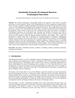
COMPETITIVE PRESSURE: A CHANNEL TO REDUCE THE OUTPUT PER WORKER GAP
BETWEEN COUNTRIES.
Stefânia Grezzana
Sao Paulo School of Economics - Getulio Vargas Foundation
Rafael Vasconcelos1
Sao Paulo School of Economics - Getulio Vargas Foundation
Abstract. Using a industry-country based approach, this study investigates the existence of an optimal
level of competition to enhance economic growth. With that in mind, we try to show that this optimal level is
different from industrialized and under development economies due to the technology frontier distance, the
terms of trade and each economy’s idiosyncratic characteristics. Therefore the difference in competition
level on an industry-country basis is a channel to explain the output per worker gap between countries.
The obtained results imply the existence of an inverted-U relationship between competition and growth.
Controlling for the terms of trade and the industry-country fixed effect, we have that if the industries of the
developing country operated under the same competition levels as that of the industrialized ones there is a
potential increase in output of 0.2-1.0% p.y in the economy.
Key-words: Competition, Economic Growth, Industry Studies.
Resumo. Ultilizando uma análise indústria-país, esse estudo investiga a existência de um nível ótimo
de competição que favorece o crescimento econômico. Com isso em mente, tentamos mostrar que esse
nível ótimo é diferente entre as economias em desenvolvimento e as industrializadas devido a distância
de cada uma relação a fronteira tecnológica, os termos de trocas e as características idiossincraticas de
cada economia. A partir disso, a diferença nos níveis de competição das indústrias-países é um canal para
explicar o gap do produto por trabalhador entre os países. Os resultados obtidos implicam na existência da
relação de U invertido entre competição e crescimento. Controlando pelos termos de troca e os efeitos fixos
sobre indústria-país, nos obtemos que se as indústrias dos países em desenvolvimento operassem ao mesmo
nível de competição das indústrias dos países industrializados o seu produto cresceria 0.2-1.0% a.a.
Palavras-chaves: Competição, Crescimento econômico, Estudos sobre a Industria.
JEL: F43, L60, O41.
Área 4 - Macroeconomia, Economia Monetária e Finanças
1
Thanks to FAPESP by their financial support. E-mail address contact: [email protected]
1
1. I NTRODUCTION
Acemoglu et al. (2006) indicates that there exist strategic alternatives to enhance growth involving
different institution structures and public policies. For these authors, developing countries should focus
their efforts accumulating physical and human capital, imitating and/or adapting technologies developed
by developed countries. These proposals would be attainable even in a situation of restricted economic
competition. The technological progress - the main engine of growth for developed countries -, however,
would be encouraged by a more competitive market structure.
Thus, this study will focus on the relationship between competition and economic growth in the same
fashion as Aghion et al. (2005) relates competition and innovation, that is, in an inverted U format. The
mechanisms which produce this relation, though, are not the same. In one hand, competition discourage
innovations by reducing the firm’s expected profit. On the other hand, competition also tends to encourage
the entry of firms with greater innovative potential2 while also induces the incumbent to innovate to maintain
its leading position. For these reasons, it is possible to obtain benefits from a greater competition level whilst
there are possible negative implications caused by its increase (Bento, 2014).
The industrial organization literature just as the Schumpeterian models argues that a a higher level of
competition would reduce the innovative firm’s profit - rent dissipation effect - in such a way that the
competition would have negative impact over the aggregate innovation rate and consequently over the
aggregate economic growth. It follows from the theoretical models of price competition and horizontal
product differentiation3 that the increase in competition inhibit the entry of new firms4 through the reduction
of post-entry profit to the innovative firm.
The same result is found in models of product differentiation in monopolistic competition environments
as well as in growth models with variety of products Acemoglu (2009). These endogenous growth models
indicate that ex post reduction of the monopoly profit discourages ex ante investments in Research &
Development (R&D). Therefore this reduce the rate of innovation as well as the long run growth of the
economies which in these models is proportional to the aggregate rate of innovation. Going back to the
theoretical models of industrial organization, the models of anticipation and innovation tend to disagree with
the previous ones suggesting a positive relationship between competition and innovation. According to this
literature, if the incumbent and the entrant firms begin an innovation race, it is possible that competition has
positive effects on growth (Aghion et al., 2009). It would depend mostly on the net effect of rent dissipation
effect and replacement effect.
From the replacement effect the entrant firm would have greater incentive to innovate as it would make
possible the transition from zero to a positive profit. Meanwhile, by innovating the incumbent firm replaces
its own profit for the monopoly one. On the other hand, the rent dissipation effect implies that the incumbent
firm would have bigger losses allowing the entry to happen than the entrant firm would if it was to give up
on entry: the incumbent would transition from a monopoly profit to a duopoly situation whilst the entrant
would abstain from getting the duopoly price and would maintain zero profit. Thus, the incentive of the
incumbent to innovate is proportional to the difference between the monopoly and duopoly profits, whilst
the entrant firm’s incentive is proportional to the duopoly profit. That means that in an environment of high
competition levels, the duopoly profit can be reduced such that the difference between the monopoly and
the duopoly profit is greater than the duopoly profit itself (Acemoglu and Akcigit, 2012). For that reason,
the incumbent invests more, ensuring that the market situation will not change and implying a positive
relationship between competition and innovation.
In summary, competition would encourage growth because it would reduce the pre-innovation profit in
a higher magnitude than that of the reduction of its post-innovation profit (Aghion et al., 2005). That is,
the competition increases the incremental profit from the innovation which takes place in order to escape
post-entry market competition, the so called escaping competition effect. The dominant effect - either
the escaping competition or the rent dissipation - will depend on the technological characteristics of each
2
Aghion and Griffith (2008) states that the rate of innovation is higher on entry firms since they must have at least the same
technological level of the incumbent. Thus the search for the technological level of the incumbent generates, on average, a higher
rate of innovation among entry firms.
3
The Hotelling linear model and the circular version of Salop (1977) apud Aghion and Griffith (2008).
4
We take this as having attenuating effects over the technological progress.
2
industry in the economy, which in turn depends on the technology gap between the firms operating in each
sector.
Given this relationship, Aghion et al. (2005) establishes a theoretical relationship between competition
and growth. For this, the authors distinguish the pre and post-innovation profits and argue that an increase
in competition has an ambiguous effect on the aggregate innovation rate and that this effect depends on the
market structure of each industry. This would justify an inverted U relationship between competition and
innovation. There would be a dominant escaping competition effect for low levels of competition and a
dominant schumpeterian effect for high levels of competition. Following the model constructed by Aghion
et al. (2005), within the same industry there are firms with different technological levels, because even the
technological laggards have non-negative profit. Thus, to some extent for each industry we have two states:
(i) the sector is leveled - neck-and-neck - that is, firms have similar cost structures and technologies and
therefore have the same profit; and (ii) the sector is unleveled - Stackelberg competition - where the leading
firm has a higher technological level obtaining greater profit than the follower firms.
The balanced aggregate innovation rate and, as a result, the growth rate of the aggregate output, will
depend on the fraction of time that each sector remains level or unleveled. This is the so called composition
effect. Thus, according to Aghion et al. (2005), if the the fraction of firms in the leveled or unleveled
industry in economy is an exogenous parameter, the higher the fraction of neck-and-neck industries in the
economy, the greater the positive effect competition will have on the aggregate rate of innovation.
Crucially the quest for innovation is the firm’s search for higher profits. So in this study we will show
that the search for greater profits affect the degree of competition. Moreover, the industrialized and the
developing countries’ industries grow differently and, to some extent, their growth depend on the different
levels of competition among them. This relationship would be different because the industries-countries
have different levels of technology as well as because of the fact that the economies have different terms of
trade. Thus, it is reasonable to think that the industry structure of each country has an impact on the rate of
innovation, on competition and on the difference between the economies’ growth rates.
Therefore, the aim of this study is to clarify how the degree of competition and the growth rate of
the product are correlated. This correlation would be distinct and dependent on the distance that the
industry-country is to the technological frontier and the idiosyncrasies of each industry-country. We show
the effect of varying the competition level on the growth of product for the industries in the developing
countries. In other words, we compute what would be the gain in terms of growth if each industry in the
developing countries had on average the same level of competition as that of the respective industry in the
industrialized countries. Thus, the difference in competition industry-country level would be a channel to
explain the output per worker gap between countries.
Our results imply that there is an inverted-U relationship between competition and the growth rate
of output across industries-countries. The same is also distinctive among industrialized and developing
countries. Given that on average the industries in the industrialized countries have higher levels of
competition, with appropriate controls variables if the respective industries in developing countries had
the same level of competition as of the first the growth rate of their product would rise 0.2-1.0% p.y. Note,
therefore, that this study contributes to the literature by presenting an additional channel to explain the
difference between the Gross Domestic Product (GDP) per capita of developed and industrialized countries.
In summary, we state that the difference in the output per capita in these countries can also be related to the
difference in the level of competition in each country and the mechanisms that determines it. Not only it
affects the profitability of each firm but it also affects the incentives to rise the technological level, which
in turns affect the rate of growth between countries. Finally, while keeping the focus on manufacturing
sectors, we predict that the same would happen with other industries.
The rest of the study is divided as: Section 2 presents a theoretical model that relates competition and
growth, while Section 3 describes the dataset used and the method of measurement for the key variables. In
Section 4 we document and interpret the empirical results. The last section concludes this study.
3
2. M ODEL
The model to be presented relates competition and output growth for the industry-country. In general, it
follows the theoretical characterization used by Aghion et al. (2005) but also making use of the Acemoglu
and Akcigit (2012) approach.
There are two important differences in the model we present he as opposite to the one normally presented
in the literature. First, we don’t impose that the intermediary goods used for the domestic production of
final goods are necessarily substitutes. Second, there exists a relationship between economies in terms of
trade that increase the effects of competition on growth. The integration of these components, along with
the interaction between economies should enhance the competitive incentives of firms.
We show that there is an inverted-U relationship between competition and growth. But, this relationship
is differently across firms and industries of industrialized and developing countries and that explains part of
the difference in GDP per capita between these groups of countries.
2.1. Environment. Consider two economies indexed by i = {A, B} with finite horizon and continuous
timing. Each one of them has a continuum of individuals with standard preferences regarding the
consumption of a final good produced domestically, which the utility function is
Z ∞
i
(1)
U C (t), t =
log C i (s) exp − ρ(s − t) ds,
t
where ρ ∈ (0, ∞). Assume that the only relationship between the two economies occur via the trade of
intermediate goods and that has no cost of transaction. Each country produces a final good Yti , which is
consumed only by domestic individuals. For this production, we use intermediate goods of domestic origin
X̃ti and/or intermediate goods of foreign origin X̄ti , whose production functions are given by
1
1 YtA = αA (X̃tA )1− + (1 − αA )(X̄tB )1− −1 ,
(2a)
(2b)
1
1 ε
YtB = αB (X̃tB )1− ε + (1 − αB )(X̄tA )1− ε ε−1 ,
where ∈ (0, ∞), ε ∈ (0, ∞) e αi ∈ [0, 1]. The intermediate good of domestic and foreign origins are not
necessarily complementaries in the production of final goods, in which case ∈ (0, 1) and ε ∈ (0, 1) for
country A and B respectively.
The aggregate production of intermediate goods in each country is then given by Xti = X̄ti + X̃ti . In
other words, the domestic production of intermediate goods divides itself between the share used for the
production of domestic final good and the exported share. We will see that the differences in performance
of the output per worker across countries are correlated with different levels of domestic and international
competition. Not only that but the competition would be correlated with differences in the technological
level, the terms of trade and the degree of substitutability in the production of final good in each economy.
In each country two domestic firms compete with each other as well as with two other foreign firms,
given the possibility of trade of intermediate goods between countries. Each firm j = {1, 2} produces
i
i
intermediate good using technology qjt
and labor ljt
inputs at time t, whose output function is represented
by
(3)
i i
xijt = qjt
ljt .
Assume each firm’s production of intermediate good is perfectly substitute, then Xti = xi1t + xi2t . The
marginal (operating) cost of production of the intermediate good is given by
(4)
i
M Cjt
i
wjt
= i ,
qjt
i
where wjt
is the wage in time period t. Suppose that this wage is identical between firms and countries,
i
wjt
= wt . This means that the difference between prices would be exclusively due to the current
technological level and the terms of trade.
4
Assumption 1. Whenever domestic firms are unleveled, domestically, firm 1 has the highest technological
level, that is
i
i
q1t
≥ q2t
.
(A1)
And so, it assumes the domestic leading position in term of technology.
The technology of each firm is given by
i
i
= λnjt ,
qjt
(5)
where λ ∈ (1, ∞) is an efficiency term identical between countries and nijt denotes the technological level
of firm. Define P̃ti as the price of domestically produced intermediate good used in the production of
domestic final good, and P̄ti as the price of the same good when traded internationally. In addition, with
no trade costs, the price of the domestic good must be equivalent to the price of the imported one in terms
of domestic currency. This is P̄tA = ρt P̃tB and P̄tB = P̃tA /ρt , where ρt summarizes the terms of trade
(exchange rate) between the two economies. The higher ρt the higher the price of the exported good from
country A and the lowest it is from country B. It that means that the profit from country A’s firms increase
with the terms of trade whilst the profit of firms in country B decays. This interaction between the markets
generates a degree of competition in terms of price between the two economies.
2.2. Static Equilibrium. Given the initial setting and equations 2a and 2b, maximizing the final good with
respect to the intermediate inputs, we get that the domestic demand for intermediate goods in each country
is given respectively by
A −
−ε
P̃t
ρt P̃tB
A
A
Xt =
(6a)
Yt +
YtB ,
αA
1 − αB
(6b)
XtB
=
P̃ B −ε
t
αB
YtB
+
P̃tA
ρt (1 − αA )
−
YtA .
Therefore the price of the domestic intermediate good in each country affect their demand for intermediate
goods. The challenge now is to determine the domestic prices for the intermediate goods and how they are
related to the technological level of each economy.
Assumption 1 and the price competition imply that in each country the price of the domestic intermediate
good is given by
wt
(7)
P̃ti = i .
q2t
From the equations 6a and 6b, we have that this level of prices implies that domestic demand for goods,
with domestic or foreign origin, depends mainly on the technological level of the domestic firm that has the
lower technological level. Thus, each firm’s j from country i profit function is given by
i i
i
xjt .
= P̃ti x̃ijt + P̄ti x̄ijt − M Cjt
πjt
We also have that each intermediate good firm can have its production divided between the internal and
external market, that is xjt = x̄jt + x̃jt . So each intermediate good firm’s profit is given by
(8)
i
i
i
= π̃jt
+ π̄jt
,
πjt
i
i
where π̃jt
represents the profit made in the internal market and π̄jt
is the profit made in the external one.
From this we have that the diferent types of profit for each firm in each country are given, respectively, by
A −nA
n
A
1−
A A
(−1)nA
2t − λ 2t
jt ,
π̃jt = wt (α ) Yt λ
A
B
εnB
A
2t −njt ,
π̄jt
= wt1−ε (1 − αB ) YtB ρ1−ε
λ(ε−1)n2t − ρ−ε
t
t λ
εnB
−nB
(ε−1)nB
B
1−ε
B ε B
2t
2t
jt
π̃jt = wt (α ) Yt λ
−λ
,
5
B
π̄jt
=
wt1− (1
A −α )
YtA
−nB
−1 (−1)nA
nA
2t
2t
jt
ρt λ
− ρt λ
.
Note that if αA = αB = 1 and = ε = 1 we fall back in the standard case presented by Aghion et al. (2005)
i
i
i
= Yti [1 − λn2t −njt ].
and so πjt
There are three important point emphasizing as direct results from equation 8 which have distincts
implications to the pattern presented by Aghion et al. (2005), Aghion et al. (2009), among others. First, the
firm j’s profit will not depend only on the technological gap between domestic firms. But also on the gap
between firms from the foreign country. The domestic firm low-tech would have zero profit in domestic
demand for intermediate good. But it could have positive profit by exporting if it had a technological level
sufficiently larger than that of the low-tech firm of the foreign country. This is due to the trade relationship
between the two economies.
Secondly, this gap also depend on the complementarity of the intermediate goods in each economy, e
ε. For example, if = ε = 1, the profit of the intermediate goods firm of the economy A is
1
A
B −nA
−n
nA
n
B
B
A
A A
πjt = α Yt 1 − λ 2t jt + (1 − α )Yt 1 − λ 2t jt .
ρt
However, the higher the substitutability of the intermediate goods in the production of final goods, the
higher the competition. To the extent that the magnitude of the profit is enhanced by this substitutability, and
any technological difference could generate a significant profit gain on selling to the internal and external
markets. Therefore, the greater would be the incentive to increase the intermediate good’s production and
raise the technological level of firms.
Lastly, the third point is that there would be a ratio in the terms of trade that would intensify (or attenuate)
the effect of the technology gap between firms and between economies. It would imply that depending on
the terms of trade and its impact on the relative prices of each intermediate good in the foreign and domestic
market we would have a situation in which the domestic country’s firm has incentive to export. Of coarse,
since it could have positive profit in the external market and despite having zero profit in the domestic
market.
From equation 8, the condition that allows each firm to exports and obtain non-negative profit from
A
B
B
exporting is given by nA
jt − n2t ≥ logλ ρt and njt − n2t ≤ logλ ρt , for firms in country and A and B
respectively5. The higher ρt the higher the price of exported intermediate good from firms in country A.
Also the greater the profit of these firms and as a consequence, the greater their incentive to sell to the
external market vis-a-vis to the firms in country B. But if ρt is sufficiently small only the leading company
in the domestic market could have a significant gain in exporting. Further note that this would not depend
on the degree of substitution between the intermediate good from the domestic or foreign country.
Proposition 1 (Existence of international trade). There will exist trade of intermediate good between two
economies if at least one firm obtains non-negative profit by selling to the external market, thus
(P1)
A
B
B
nA
jt − n2t ≥ logλ ρt ≥ njt − n2t ,
would be satisfied to at least one firm in each time period. Even the is the domestic market is under perfect competition, so there is no technological gap between
the domestic firms, they could have positive profits by exporting. Moreover, the high degree of domestic
competition increases the dynamic incentives to invest in innovation. Because each firm has an incentive to
invest in new technologies to perpetuate the leadership or establish one, in relation to at least one firm in
the foreign market.
When the domestic market is not perfectly competitive, each firm high-tech always have positive profit
by selling to its own domestic market and possibly to the external market. However, the firms obtain distinct
profits depending on the existence and size of the technological gap in relation to the domestic and external
low-tech firm. This higher profit encourages further investment in R&D to maintain the leadership in both
domestic and foreign markets. Thus the replacement effect is intensified. Given the interaction between
5
A
A
B
Curiosily, note that if nB
jt > n2t or njt < n2t then it would be necessary that ρt > 1, otherwise for any condition ρt ∈ (0, 1].
6
markets, the rent dissipation effect would also be higher than in the situation where the economies are
closed because the degree of competition is also higher.
Additionally, let µi1 denote the steady-state probability of being an unleveled and µi0 that it is leveled.
This, together with the fact that µi0 + µi1 = 1. We then define the optimal allocation or static equilibrium.
Proposition 2 (Optimum Allocation). The optimal allocation is a sequence of optimal decisions of each
∞
∗ ∞
firm j in each country i {x∗i
it }t=0 and a sequence of optimal wages {wt }t=0 for a given sequence of optimal
i
prices {P̃t∗i , P̄t∗i }∞
t=0 and an initial distribution {µ0 } of firms in each country i and each time period t. Dynamically, the low-tech firms could have some gain in investing in new technologies to increase the
technological gap in relation to the firms with even lower technological level or to become a high-tech and
thereby achieve greater profitability both domestically and in externally. Moreover, even for the high-tech
firms there is an incentive to create new technologies to further increase the gap against other firms, both
domestically and internationally.
Note that the static equilibrium provides a partial response to our problem. Firms in developing countries
have on average lower technological level, so they have lower profit, on average, than firms in industrialized
countries. This would produce lower profits and incentives to raise the technological level and thus attenuate
the long-run growth of product. Since economies interact in trade and firms in industrialized countries tend
to be more competitive, these firms generate even bigger profits - additional profits from the export market
- coming from the developing countries. This further increases the long-run output growth of firms in
industrialized countries and also increases the gap in output per worker between industries-countries.
2.3. Measure of competition. Before characterizing the equilibrium dynamic of the model, we will define
the measure of competition we used in the model and will also be used in the empirical exercise. Suppose
the two domestic firms previously characterized were in a neck-and-neck situation, if they enter in collusion
i
i
each could get a fraction σ̃t of profit as if there were a domestic leader. So we can set σ̃ti = π̃0t
/π̃1t
,
i
where σ̃t ∈ [0, 1], as a measure of domestic competition among firms, as developed by Boone (2000).
Using the same reasoning for the international market if domestic leaders are in a neck-and-neck situation
internationally and enter in collusion, they would get a fraction σ̄t of the international profit. So we can set
i
i
σ̄ti = π̄0t
/π̄1t
, where σ̄ti ∈ [0, 1), as a measure of international competition among firms. The less diverse
are the profits with and without collusion the higher is the competition which means that competition is
increasing in these measures.
We take that it is be possible to have low competition in the domestic market and high competition in
the international one. The search for export gains could lead the a race for innovation, and as a result, an
i
i
such that the above conditions
/π1t
increase aggregate activity. Define the aggregate competition as σti = π0t
we can construct it as
i
π̃ i
i π̄1t
(9)
σti = σ̃ti 1t
+
σ̄
t i .
i
π1t
π1t
In other words, the aggregate competition is the sum of the competition levels weighted by the share of
net profit obtained in each origin. Thus, the aggregate competition of each country would depend on the
domestic competition as well as the external one weighted by the relative profits obtained in each of the
sources. The higher (lower) the profit obtained with the internal market relatively to total income, the higher
(lower) is the weight of internal competition on aggregate measure. A similar argument is valid for the profit
derived from the external market.
i
2.4. Dynamic Path and Equilibrium. Now we characterize the dynamic equilibrium. Define zjt
is the
i
i
i
innovation rate of the firm such that zjt = F hjt , where hjt is the number of researchers devoted to R&D
i
in each firm. To increase its technological degree each firm incurs a cost of R&D given by wt G zjt
. This
i
firm moving one technological step ahead with a Poisson hazard of zjt . Addionaly, suppose F (·) is an
i
i
i 2
increasing and strictly concave function subject to the Inada conditions and G zjt
≡ F −1 zjt
= (zjt
) /2.
Considering the one-step case if in a period of time ∆t a high-tech firm is successful in innovating, then
i
i
i
i
it ratifies its domestic leadership and its level of technology goes from qjt
= λnjt to qjt+∆t
= λqjt
. On
the other hand, if the low-tech firm is successful in innovating it becomes a high-tech firm domestically
7
i
i
i
i
. Considering the interaction with the
= λn−jt to qjt+∆t
= qjt
and its technological level goes from q−jt
external country, depending on the size of the innovation produced, on the terms of trade and on the degree
of substitutability in the production of final goods, each domestic firm could increase its profit from the
intermediate goods exported through the innovation. This would occur even if the domestic firms are under
perfect competition.
Proposition 3 (Dynamic Equilibrium). The Markov Perfect Equilibrium is given by a optimal sequence
∗i
∗i
∗i ∞
∗i ∞
∗i ∞
{zjt
, P̃t∗i , x∗i
jt , wt , Yt }t=0 such that (i) a sequence of price {P̃t }t=0 and production {xjt }t=0 imply that
∗i
∞
∗i ∞
{zjt
, P̃t∗i , x∗i
jt }t=0 satisfies the equations 6 and 7; (ii) {zjt }t=0 maximizes the expected profit of each firm
∗i ∞
∗i ∞
given the aggregate output {Yjt∗i }∞
t=0 , wages {wt }t=0 and the choice of costs with R&D {zjt }t=0 ; (iii) the
aggregate output {Yjt∗i }∞
t=0 is given by the equation 2; and (iv) the labor market is in equilibrium in every
time period given the sequence of wages {wt∗i }∞
t=0 . We now define Vjti as the steady-state value of each firm of country and rt as the opportunity cost of
production. Specially, V0ti would refer to the situation in which there is no technological gap between
industries in country, that is ni1t = ni2t . Thus, each firm’s decision to innovate for each country can be
summarized by the following Bellman functions
(10a)
i
i
i
i
i
(V1ti − V0ti )
− V1ti ) − z2t
(V1t+1
) + z1t
− wt G(z1t
rt V1ti = π1t
−i i
−i i
ξt (V1ti − V0t−i )
−z1t
ξt (V1ti − V1t−i ) − z2t
(10b)
i
i
i
i
i
rt V2ti = π2t
− wt G(z2t
) + z2t
(V0t+1
− V2ti ) − z1t
(V2ti − V0ti )
−i i
−i i
−z1t
ξt (V2ti − V1t−i ) − z2t
ξt (V2ti − V0t−i )
(10c)
i
i
i
i
rt V0ti = π0t
− wt G(z0t
) + z0t
(V1ti − V0ti ) + z0t
(V2ti − V0ti )
−i i
−i i
−z1t
ξt (V0ti − V1t−i ) − z2t
ξt (V0ti − V0t−i )
where ξtA = ρt and ξtB = 1/ρt . For the domestic leader - equation 10a - the first and second term
represent the operational profit minus the cost with R&D, the third and fourth are the cost of maintaining
its leading position in the domestic and international markets respectively, the last term represents the cost
of maintaining its leadership in the face of the follower in the international market. Note that the ratio value
functions is readjusted by the terms of trade.
For the domestic follower - equation 10b - the intuition is similar. The operational profit minus the
cost with R&D, summing the gains of becoming the domestic leader and the gains of having some sort of
leadership in the international market. Note, however, that for the domestic follower the profit from the
domestic market is zero. Still, the firm may exhibit some positive profit by selling to the external market if
there is a sufficiently high technological gap at least in relation to the foreign country’s follower. Otherwise,
this profit is also zero.
Equation 10c presents the domestic neck-and-neck situation with similar intuition as of the follower
one. It emphasizes that the domestic firms may be in a neck-and-neck situation domestically, but still in
the leadership position facing the foreign companies. Therefore, for them it would be worth increasing
spendings with R&D to maintain the leadership (domestic market) or conquer it in the foreign market. This
would occur even if the neck-and-neck situation was held in the internal market, that is the replacment effect
in the foreign market could be bigger than the effect than the rent dissipation effect in the domestic market.
Assume for simplicity that wt = β = 16. Using the fact that each firm chooses its R&D spendings that
maximize its current value from the system of equations 10 for each country the first order conditions imply
that
(11a)
i
i
z1t
= V1t+1
− V1ti ,
(11b)
i
z2t
= V0ti − V2ti ,
(11c)
i
z0t
= V1ti − V0ti .
6
See Aghion et al. (2005) for more details.
8
From the system of equations in 10 and 11 we have a system with 12 equations. Using our measure of
competition σ we can obtain, recursively,
q
B
A
A 2
A
(12a)
),
+ (z1t
z0t = −Rt + (RtB )2 + 2(1 − σtA )π1t
(12b)
A
z2t
=−
A
z0t
+
A
z1t
q
A 2
A 2
A
A
A
)
) + (z1t
+ (RtB )2 + 2 (1 − σtA )π1t
+ (z0t
− π2t
+ π0t
B
z0t
= −RtA +
(12c)
(12d)
+
RtB )
B
z2t
=
B
−(z0t
+
B
z1t
+
RtA )
+
q
B 2
B
),
+ (z1t
(RtA )2 + 2(1 − σtB )π1t
q
B 2
B 2
B
B
B
),
) + (z1t
+ (z0t
− π2t
+ π0t
(RtA )2 + 2 (1 − σtB )π1t
i
i
)/ρt can be understood as the opportunity cost expanded by the foreign firms’
+ z2t
where Rti = rt + (z1t
spendings with innovation in terms of local currency.
i
The amount spend in the increase of the technological level zjt
is decreasing on the degree of competition
σt , similar to Aghion et al. (2005) and Acemoglu and Akcigit (2012). However, adding the international
competition, the amount spend with innovation will dependent on the amount foreign firms spend with it
i
in terms of the national currency. This is another reason why z1t
tends to be non-null. That is, even if the
firm has the domestic leadership but not the international one there would be some gain in increasing the
technological level. For this reason the lazy monopolist effect tends to be lower in the situation where there
is trade interaction between economies due to the higher degree of competition between firms. Moreover,
even the domestically low-tech firms have a greater incentive to invest in new technologies to profit in
potential foreign markets.
i
+
From what we have showed the aggregate rate of innovation in each economy is given by: Iti = µi1t (z1t
i
i
i i
i
z2t ) + 2µ0t z0t , where µ1t + µ0t = 1. In steady-state the expected value of the spendings with innovation
must be equivalent to the share of leveled and unleveled firms. Which means,
i
i
i
µi1t (z1t
+ z2t
) = 2µi0t z0t
implying on
i
i
i
z1t
+ z2t
2z0t
i
and
µ
=
1t
i
i
i
i
i
i
2z0t
+ z1t
+ z2t
2z0t
+ z1t
+ z2t
and we rewrite the aggregate rate of innovation in each country as:
µi0t =
Iti =
(13)
i
i
i
4(z1t
+ z2t
)z0t
.
i
i
i
2z0t
+ z1t
+ z2t
Note that from system 12 and equation 13 the aggregate rate of innovation is a profit function. It is also,
implicitly, a function of the degree of competition between firms and countries given the optimal allocation
of the production factors (as seen in the above subsection).
2.5. Unbalanced Growth Path. From what has been characterized in the previous sections the growth
rate of each intermediary goods sector is represented as
gXti = ιit gX̄ti + (1 − ιit )gX̃ti ,
(15’)
where ιit = X̃ti /Xti represents a fraction of the intermediary product domestically commercialized. From
equations 3 and 13 we have that this rate is also given by
i
i
i
+ z2t
) + 2µi0t z0t
log λ
(14)
gXti = µi1t (z1t
Thus, the output growth of each firm and industry depends on each firm’s production weighted by the
distribution of leveled and unleveled firms in each country. Moreover, this growth would depend on the rate
of innovation that, by construction, depend on the degree of competition in each industry-country. From
equations 2a and 2b the output growth rate is given by
(15a)
A
A
gYtA = λ−n2t ηtA gX̃tA + [λn2t ρt ]−/ε (1 − ηtA )(1 − αA )gX̄tB
9
(15b)
B
B
gYtB = λ−n2t ηtB gX̃tB + [λn2t /ρt ]−ε/ (1 − ηtB )(1 − αB )gX̄tA
where ηti = X̃ti /Yti represents a fraction of domestic intermediary product used as input to the domestic
production of final goods.
Therefore, there are three components on the growth rate of each country’s final product which depend on
the competitive structure of the industries-countries. The first, the price effect arising from the technological
gap; the higher the domestic gap the higher the output growth rate. In this case, the leading firm would have
higher profitability and thus greater incentives to invest in R&D to further increase its profits. Therefore,
the increase in the domestic level of competition inhibit the aggregate growth because it would reduce the
technological gap, the profits and, dynamically, the firms’ innovative incentives. That means that the search
for rent dissipation effect would increase the domestic production of final goods.
Second, the economic output growth rate i is increasing in the sum of the firms’ technology growth rate
i
weighted by quantity produced by each of them in the total domestic production of the final good, i.e., gX
.
t
The interaction between the economies results in the existence of a spillover effect in terms of economic
growth due to the effect of export growth. Note that the above effects are weighted by each good demanded
fraction in the domestic production of final good, ηti . If ηti = 1, there would be no interaction between
economies and the aggregate output would be similar to that developed by standard literature gYti = gXti .
Finally, the terms of trade, ρt raise the aggregate output growth rate of country A and decrease the
rate of country B. The higher the terms of trade the greater the value received from the exported good
by the intermediate producer of country A, which means that he makes higher profits in the event of any
technological advantage that provides him with non-negative profits.
In summary the competition effect would be implicitly determined in each one of these terms in that
the optimal allocation described in the previous subsection implies the existence of non-negative profits for
high-tech firms. Thus, through prices, terms of trade or dynamic incentives to raise the technological level
(summarized in this quest for profit) competition affects the growth rate of each economy.
Proposition 4 (Existence of unbalanced growth path). The Markovian equilibrium guarantees that there
is a unique unbalanced growth path equilibrium where the different firms of intermediate goods grow at
distinct and constant rates. Proposition 5 (Growht path). Given the optimal allocation established by equations 2, 6 and 7, the system
of equations established by 13, 15’ and 15 trace each country’s economy’s equilibrium path. Unlike the Aghion et al. (2005) the domestic economy’s growth rate of the final product is increased
by an interactive effect with the external market. In short, from equation 14 we estimate gYti = f (σti ),
where f (·) would have an inverted U shape different for each country due to the escape competition and
the Schumpeterian effects. For low levels of competition the escape competition effect would dominate the
relationship, because the expected gains of increase in profits is relatively high. Any increase in competition
- domestic or international - would cause a rise in profits. Thus, each firm has an incentive to invest in
new technologies to further increase its profits. The increased production of intermediate goods and the
increase of technology imply an upward trend in the aggregate output. For high levels of competition,
the Schumpeterian effect tends to dominate because the expected increase in profits is increasingly low or
zero. The increased competition creates a race for production - to meet domestic and international markets
demands - and the generation of new technologies to reduce marginal costs. Thus, profitability decreases in
competition for high levels of competition and of certain technologies saturation.
There are other two important points about the model. The first refers to the degree of substitutability
between goods in the production of final goods for countries A and B. If > ε the greater will be the
positive effect of import variations over country A’s aggregate output vis-a-vis if < ε of country B. If
the production of the final good has greater substitutability (or complementarity ) in inputs for country
A than B then there is an equalization in the prices of inputs such that for the same level of domestic
intermediate production intended to the domestic market, the value of the variation of imports rises. Which
in the proposed substitutability case causes the growth of the aggregate product. The same would occur
if the production in country A was more complementary than the production in country B. If < ε the
10
smaller the positive effect of the changes in imports on the aggregate product of country A vis-a-vis if > ε
of country B. In this case, intuition is similar.
The second point relates to the terms of trade ρt . Although it raises the relative price of the exported good
of firms in country A and, consequently, their profits vis-a-vis of firms in country B, the prices of domestic
goods equalize with imported goods and this implies a reduction of growth in country A and an increase in
country B. In the described situation, although it coexist with the increase of country A’s firm’s profit the
growth would decay because for the same level of competition and technology there would be a reduction
of the value of changes in imports. Moreover, the effect of terms of trade would be enhanced by the degree
of substitution described above.
In summary from the framework presented here, competition and growth would be correlated in a
inverted-U shape mainly due to the interaction of the Schumpetarian and escaping competition effects.
In the following session we will seek to corroborate empirically the proposed inverted-U relationship
between competition and growth, as well as demonstrating that this inverted-U differs between industries
in developing and industrialized countries.
3. DATA AND MEASUREMENT ISSUES
In this section we will describe the data used in our empirical exercise as well as the key variables used
in the analysis.
3.1. Data. For the comparison between industry-country we used two databases of United Nations
Industrial Development Organization (UNIDO).
The Industrial Statistics Database at the 4-digit level of ISIC Code (Revision 3) contains annual time
series data for 1990 to 2010 and for 135 countries. The data is arranged at the 4-digit level of the
International Standard Industrial Classification of All Economic Activities (ISIC) Revision 3 pertaining
to the manufacturing sector, which comprises 151 manufacturing categories. The database contains
information on the number of establishments, employment, wages and salaries, output, value added, gross
fixed capital formation, and number of female employees. The initial capital stock is imputed as the average
of gross fixed capital formation in each sector and country. The data is stored in current US Dollars.
The other database used is the Industrial Demand-Supply Balance Database at the 4-digit level of
ISIC Code (Revision 3) pertains to the manufacturing sector and contains data at the 4-digit level, which
comprises 127 manufacturing industries. These database contains information on imports and exports from
94 countries/areas for the period 1990-2010. It is important to mention that period coverage as well as
item coverage differ from country to country. The database contains annual time-series data on the imports
and exports from industrialized, developing and emerging industrial economies. From these variables we
construct the total exports and total imports for each industry-country.
Taking this two databases we have a panel with annual data from 121 sub-sectors of the manufacturing
sector from 65 countries between 1990 e 2010. Lastly, the nominal variables are deflated by the total
product of the manufacturing sector of each country in 2000 year. For some tests we also use aggregate
data summarized by Feenstra and Timmer (2013) and Botero et al. (2004). We will be explicit about this
additional data as we make use of them throughout the study. It is important to emphasize that we will be
working with a small panel that contains missing data. For that reason, specially in the linear regression
cases, we will make use of methods to mitigate this problem such as the forward orthogonal deviations
suggested by Arellano and Bover (1995).
3.2. Measurement issues.
3.2.1. Growth value added. We define the rate of output growth of firms in the intermediate sectors in the
standard fashion, as the intertemporal difference of the logarithm of value added for each industry-country
i
in time, gti = ln Xti − ln Xt−1
.
3.2.2. Exchange rate. We use two measures of exchange rate. The first is constructed from the output value
in terms of national currency and of U.S. dollars. So we have a measure of terms of trade ranging from
industry-country and also over time. In the second we use the exchange rate provided by the Feenstra and
Timmer (2013) that relates domestic currency and U.S. dollars, but that rages only in the country and time.
11
Our base models are focused on the use of the first measure (terms of trade), whilst the second will be used
to check for measurement error, because the variability of the same industry in different countries could be
due to changes in prices or other unobservable costs and not necessarily in the terms of trade.
3.2.3. Measures of competition. We use two index of competition. The first, from equation 9, establishes
a level of competition that depends on production for the domestic and the external markets. For each
sector and year we calculate the maximum across all countries and measured how far each industry-country
is from the maximum, in terms of profit, in the domestic and external markets. To avoid cases where
a industry-country has an excessively higher profit than the average, we have alternative measurements
calculated based on the 90 and 75 percentile. We also calculate using the U.S. industries as the benchmark7.
The second measure is the Competitive Industrial Performance (CIP) index developed by UNIDO.
Fundamentally this index combines four measures of competition that vary between countries-sectors.
It is noteworthy that in our empirical exercise we expect the results to be better for the full sample when
we use the basic measurement. For the subsample of developing countries, however, we expect the results
to be be better when we use the 90th and 75th percentile as the benchmark to the competition measure.
This is because the profitability of firms in developing countries is low relatively to the profitability in the
developed countries, which would distort our measure of competition. This would also happen when for
some industries there are industries-countries with excessively high profitability, usually associated with
abundance of a commodity/natural resource. When using the 90 or 75 percentile we do not exclude an
excessive number of industries from developing countries and we do not distort competition between them,
which makes these alternative measures fit for use. So we reduce the impact of atypical situations and also
generate greater variability of competition between industries-countries .
In figure 1 we showed a correlation between the average growth rate of the output’s value added of
each industry-country and the average of each competition index. Firstly, the competition in the industries
of industrialized countries is on average higher than the ones in developing countries. Moreover, for the
same level of competition the output growth rate varies mainly in industries of the developing countries8.
i
When we use the basic measure of competition, σjt
, we have a negative relationship between competition
and growth, which suggests that the schumpeterian effect is strong in this correlation. But the inverted-U
appears in the subsample of industries in developing countries only changing the baseline.
4. E MPIRICAL INVESTIGATION
4.1. Econometrics methods and issues. The existence of the inverted-U and the difference in optimal
levels of competition and growth will be tested in this section. Our goal is to show that the industry-countries
have different levels of competition and this have implications on their output growth rates.
i
i
and the competition index σjt
The equation to be estimated relates the growth rate of value added gjt
i
i
i
i
such that gjt = f (σjt , xjt , ujt ). Where xjt is a vector of control variables such as time and industry-country
dummies, and uijt is the error component that has standard properties. In addition, xjt includes observable
variables that affect the output growth rate of industries-countries but are not explicit in the model such
as the logarithm of initial GDP, investment and human capital. Additionally, we will test the effect of
property rights - which would increase the incentive to raise the technological level thus rising competition
-, labor regulation - which enhance profits by making labor less costly -, and the effect of civil rights - which
contribute to control the different institutional structures in addition to serving as proxy for property rights.
Controlling for variables that affect the output growth rate of industry-country and are not related to
competition, we show that there is an inverted-U relationship between competition and growth and that it
is different in developing versus developed countries. We have some challenges on the econometric point
of view such as heterogeneity and nonlinearity of parameters, cross-section dependence, endogeneity and
unobserved and constant-in-time effects for each industry-country (Arellano and Bover, 1995; Bond et al.,
2010; Ciccone and Papaioannou, 2010).
7
Ciccone and Papaioannou (2010) states that normalizing the explanatory variable with respect to an industry-country attenuates
the bias resulting from the variation within each country.
8
Probably due to some comparative advantage in a specific sector. For example, the oil industry in Venezuela.
12
We first estimate the following equation
(16)
2
gist = ασist + βσist
+ γEit + δxist + uist ,
where s = {1, . . . , S} index industries and i = {1, . . . , N } index countries. The variable Eit is the
exchange rate and xist is a vector of control variables that also include industry, country and time dummies.
This vector can include (depending on the specification) the logarithm of the 1990 GDP to control for
the wealth and the economic development of each country. Note that we could index the variables by j
firms instead of s industries for the N countries as presented in the model. Our observation unit will be
on the industry-country level because we are interested in the implication of competition on this level of
aggregation. From the econometric point of view this choice generates a smaller variability in the interest
variables but we will try to attenuate this problem with the methods suggested by Ciccone and Papaioannou
(2010).
We will also introduce a few control variables: (i) an index of human capital per person based on years of
schooling and returns to education (Feenstra and Timmer, 2013) to control for the effect of human capital;
(ii) a measure of flexibility in the labor market (Botero et al., 2004) that would affect the reallocation of
labor and consequently the efficiencies and profits across industries-countries; (iii) and an index of civil
rights to control for the effects of each economy’s institution on the relationship between competition and
growth (Botero et al., 2004).
First, we estimate OLS regressions using each of the proposed competition index for the full sample and
then for each subsample of countries (industrialized vs. developing). We also know that industry-country
output growth and competition are endogenous. We will use the lag of each control variable previously
described as instruments as well as the exchange rate. We use this instruments to estimate a dynamic
panel method as suggested by Arellano and Bover (1995) and Blundell and Bond (1998). Furthermore, the
Arellano-Bond GMM estimator enable the treatment of two other issues: (i) industry-country fixed effects
correlated with the dependent variables, and (ii) the fact that we are working with a small panel. The fact
that we use annual data of industries-countries may cause the result to reflect time-series cyclical behavior
and not that of the long-run which we would like. Therefore, the use of dynamic panel enable the filtering
of high frequency fluctuations.
2
We expect the OLS and GMM estimates of σist to have positive sign and the ones for σist
to have a
negative sign, which characterizes the inverted-U shape. From figure 1, we also expect that for developing
countries this inverted-U has a lower peak and higher positive skewness than the industrialized ones. From
the model, the exchange rate should present a positive sign because the higher the exchange rate the lower
the price of the domestic good in the international market making this good more competitive in terms
of price. This would generate a greater profit expectation and, finally, a higher output growth rate of the
resulting industries-countries.
4.2. Basic results. Table 2 reports the estimates from the panel regression of equation 16 taking into
account the whole sample of countries between 1990 and 2010 not worrying if the country is developing
or industrialized and without controlling for this fact (this will be addressed in the next subsection). We
emphasize that the equations were also estimated in real terms and we obtained the same pattern of results.
In columns (1) we use as explanatory variables only our variables of interest - exchange corresponds to
the terms of trade, competition index e competition index2 are the competition index and the square of the
competition index, respectively. For all specifications the competition index is defined in two fashions: σ
and CPI, as described in the previous section.
The coefficient estimates associated to the variables competition index and competition index2 are
statistically different from zero with positive and negative signs respectively. This correspond to the
inverted-U format described by the model. The effect of variable exchange also meet our expectations.
The rise in the terms of trade (or exchange rate) would have a positive effect on the output growth rate of
each sector-country to the extent that the domestic products would be relatively cheaper abroad and so, for
the same level of competition there would be an increase in the output growth rate of the sector.
In columns (2) we include as control the difference of the logarithm of GDP. This variable control
the economy’s dynamic behavior such as growth of the service and agriculture sectors (Ciccone and
Papaioannou, 2010). Columns (3) controls the effect of changes in the efficiency of the employed worker
13
because of differences in human capital. In columns (4) we include the logarithm of GDP in 1990.
Following the literature, we have that this variable controls the initial differences in the production structure
and economic development of countries. The inclusion of the latter variable affects only marginally the
magnitude of the coefficients of interest for both specifications of the competition index. Columns (5)
contain all controls described previously. These controls are significant, both individually and jointly and
present the expected sign.
The results indicate that the inverted-U relationship between growth and competition exists and persists
the inclusion of several different control variables as well as changes in the estimation method - Panel A and
Panel B. Of the control variables, the log of the initial GDP, variable which capture the country’s economic
development have a strong effect on this relationship. Furthermore, the relationship holds for different
specifications of the competition index. All estimates were also tested using the aggregate exchange rate
and the results also hold the same pattern.
It is noteworthy that these results (for the OLS case) have no causal relationship to the extent that
competition is clearly endogenous. The theoretical model itself establishes it. Therefore, we use the lag of
the explanatory variables in the dynamic panel method. In this method, the obtained autocorrelation is high
in all specifications, especially for the first lags, as stated by the Arellano-Bond test for zero autocorrelation
in first-differenced errors. We also can not reject the Sargan test of over-identifying restrictions. Thus, the
instruments used are strongly correlated with the endogenous variable and, moreover, can not be statistically
rejected, which means that the results from the dynamic GMM panel are also valid.
4.3. Developing versus Industrialized Economies. In order to establish the different impacts of
competition on growth in developing and industrialized countries, we stratified the sample into two groups
according to the countries’ economic development using UNIDO’s classification. We will investigate if
indeed the relationship is maintained in the different groups of countries and also what would be the gain
in terms of growth for the industries in the developing countries if the degree of competition was elevated
to the same level of the respective industries in industrialized countries.
Our hypothesis is that the Schumpeterian effect should occur more rapidly in the industrialized economies
that tend to invest more in developing new technologies than in developing economies whose technological
progress tends to occur via imitation and incorporation of new technologies. This is because the industries
that are more distant from technological frontier tend to benefit more from spillover effects of the technology
available in the global technological frontier.
Columns (1) and (5) of table 3 replicate the specification (5) in table 2 using the competition indexes σ
and CPI respectively, but segregating between developing and industrialized countries. In both subsamples
the results are qualitatively similar, except for the dynamic GMM panel specification of CPI in developing
countries, where the coefficient of interest does not maintain the expected sign. These results corroborate
what was observed on figure 1 and show that, on average, there is an inverted-U relationship for many
measures of competition and it is distinct among industries-countries.
Following Ciccone and Papaioannou (2010), in column (2) we report the estimates for the case in which
the U.S. manufacturing sector is excluded from the regressions and it is used as benchmarks for each
respective industry. The results are significant and as expected for panels A and B, in the case of developing
countries. For the subsample for industrialized countries, however, the number of observations for this
measure of competition drops substantially due to this exclusion of the U.S. industries.
Finally, in columns (4) and (5) we tested two additional specifications for the competition index. We
changed the benchmark of the industry failing to consider it the United States manufacturing sector - usa
columns (3) - or the maximum of each industry - σ columns (1) - substituting it by the 90th and 75th
percentiles of the output distribution of each industry. Note that now the reference country is changing
between industries. In the case of the static panel, we realized that the results remain significant and with
the expected sign. That means that using various measures of competition and control variables there
would exist a relationship between competition and growth and this relationship would differ between the
industries of developing and industrialized countries.
In table 4 we performed a similar exercise as in table 3 adding as a control the employment laws index and
the civil rights index. We expect the industry-country growth to be increasing in both variables to the extent
that the more flexible the labor market the better tends to be the allocation of labor and the better should
14
be the performance of the industry-country output. Moreover, the quality of institutions - summarized by
the civil rights index - should reveal the impact of the existence of property rights which should increase
the dynamic incentives to innovation, and legal soundness in favor of a more competitive market structure
implying that the rent dissipation effect was more blunt. However, this pattern was not significant and
consistent in the estimates. Thus, it is not possible to state conclusively the effect of these variables on the
relationship between competition and growth.
Again the autocorrelation is high in all specifications and subsamples, specially for the first lags, even in
the exercise that we include the employment laws index and the civil rights index as control. We also can
not reject the Sargan test of over-identifying restrictions. Thus, we have that the instruments used for the
subsample are also correlated with the endogenous variable and can not be statistically rejected. Again, the
results used in the dynamic panel remain valid. Furthermore, all of these estimates were also tested using
the aggregate exchange rate and the results showed the same pattern.
In summary, there is an inverted-U relationship between competition and growth and it is different
between developing an industrialized countries. We now verify what would be the gains of economic
growth to the manufacturing sector of the developing countries would have if they had the equivalent level
of competition of the manufacturing sector of the industrialized countries as well as similar economic
conditions (see figure 2). Figure 2 has been parameterized in accordance with the values estimated in the
dynamic panel. Thus, for each given level of competition any difference between the growth rates reflects
how much economic growth would that country gain compared to the other group of countries.
Primarily, as already mentioned the inverted-U appears in all specifications and estimation methods of σ.
Furthermore, the simulations imply that the increase in σ in the industry-countries of developing economies
would not reduce the difference of your output gap in relation to industrialized economies. However, for this
measure of competition we can not affirm that the optimal level of σ in developing countries is higher. This
is so because in the situation where competition results in the greatest growth of value added the difference
between the growth rates would still be -0.6% against the industries in developing countries.
However, when we use relative measures we see significant changes. At the same level of competition
the output growth rate would be higher in the developing countries industries. Thus, when we exclude
some excessively disparate industries (in terms of value added), the increased competition would reduce
the output gap between industries in the developing and industrialized countries. However, the magnitude
of this reduction would have the shape of the inverted-U. Once we control for economic development,
human capital and economic growth as a whole, the figure 2 tells us that for low levels of competition its
elevation would have a greater effect on developing economies than on industrialized ones. Nonetheless, as
the competition increases the gains become more restricted, even though there is still some improvement in
relation to the industrialized countries.
In quantitative terms, the difference between the growth rates across industries-countries when the
competition index takes the value 0.5 is equivalent of 0.224%, 0.585% and 1.035%, to σ usa, σ p(90)
e σ p(90), respectively, in favor of developing countries industries. That means that when we exclude
some outliers industries and we control for economic development, human capital and momentary
growth rate of each country, the increased competition among industries-countries tend to enhance the
industry-country output growth for developing economies in a higher magnitude than the industrialized
economies. Moreover, our results indicate that the optimal level of growth is greater for developing
countries. In table 1, we show the gains in terms of economic growth per year to the manufacturing
sector of the developing countries would have if they had the equivalent level observed of competition
of the manufacturing sector of the industrialized countries as well as similar economic conditions. Thus,
according this table, the manufacturing sector of the developing countries accumulate an increase of about
4-6% between 1990-2011, if they had the equivalent level observed of competition of the manufacturing
sector of the industrialized countries.
5. C ONCLUSION
This study attempted to show how competition and output growth are related. Departing from the
theoretical framework developed here, this correlation would be different and dependent on the distance
that each industry-country is to the technological frontier and on the terms of trade.
15
Our results imply that there is an inverted-U relationship between competition and the growth rate of the
output across industry-countries using a competition index based on relative profits of industry-countries.
We also find that this relationship is distinct among developing and industrialized economies. Since on
average the industries in the developed countries tend to present higher levels of competition even when
we control by the terms of trade and the characteristics of each industry-country, if each industry in the
developing countries had the same level of competition of the respective industry in the developed ones, we
estimate that their product growth would rise substantially.
We present here a channel to explain the difference between output per capita across countries.
Industrialized countries tend to have more competitive markets, so there is greater dynamic incentives to
raise their production. Both by developing new and better technologies that reduce costs and raise profits
and also by searching new consumer markets given the possibility of gains in international trade. However,
in developing countries the low technological level, as well as the productive inefficiencies and idiosyncratic
malfunctioning of the production system would result in less competitive industry-countries and under
determined output growth rates Acemoglu et al. (2006). Lastly, it would contribute to the maintenance of
the gap in the per capita GDP between economies.
Finally, it’s worth to mention that from the point of view of corroboration of the constructed theoretical
framework, we are estimating a linear relationship when the parameters of the theoretical model itself
indicate a non-liner relationship, making this the main focus regarding the next steps on this work. We
plan to estimate a non-linear relation that relates the different measures of competition used here, and thus
ascertain how the results behave.
R EFERENCES
Daron Acemoglu. Introduction modern Economic Growht. Princeton University Press, 1 edition, 2009.
Daron Acemoglu and Ufuk Akcigit. Intellectual property rights policy, competition and innovation. Journal
of the European Economic Association, 10(1):1–42, 02 2012.
Daron Acemoglu, Philippe Aghion, and Fabrizio Zilibotti. Distance to frontier, selection, and economic
growth. Journal of the European Economic Association, 4(1):37–74, 03 2006.
Philippe Aghion and Rachel. Griffith. Competition and growth: reconciling theory and evidence. The MIT
Pres, 2008.
Philippe Aghion, Nick Bloom, Richard Blundell, Rachel Griffith, and Peter Howitt. Competition and
innovation: An inverted-u relationship. The Quarterly Journal of Economics, 120(2):701–728, May
2005.
Philippe Aghion, Richard Blundell, Rachel Griffith, Peter Howitt, and Susanne Prantl. The effects of
entry on incumbent innovation and productivity. The Review of Economics and Statistics, 91(1):20–32,
February 2009.
Manuel Arellano and Olympia Bover.
Another look at the instrumental variable estimation of
error-components models. Journal of Econometrics, 68(1):29–51, July 1995.
Pedro Bento. Competition as a Discovery Procedure: Schumpeter Meets Hayek in a Model of Innovation.
American Economic Journal: Macroeconomics, 6(3):124–52, 2014.
Richard Blundell and Stephen Bond. Initial conditions and moment restrictions in dynamic panel data
models. Journal of Econometrics, 87(1):115 – 143, 1998. ISSN 0304-4076.
Steve Bond, Asli Leblebicioglu, and Fabio Schiantarelli. Capital accumulation and growth: a new look at
the empirical evidence. Journal of Applied Econometrics, 25(7):1073–1099, November/ 2010.
Jan Boone. Competitive pressure: The effects on investments in product and process innovation. RAND
Journal of Economics, 31(3):549–569, Autumn 2000.
Juan Botero, Simeon Djankov, Rafael Porta, and Florencio C. Lopez-De-Silanes. The Regulation of Labor.
The Quarterly Journal of Economics, 119(4):1339–1382, November 2004.
Antonio Ciccone and Elias Papaioannou. Estimating Cross-Industry Cross-Country Models Using
Benchmark Industry Characteristics. CEPR Discussion Papers 8056, C.E.P.R. Discussion Papers,
October 2010.
Robert Inklaar Feenstra, Robert C. and Marcel P. Timmer. The next generation of the penn world table,
2013.
16
F IGURE 1. Growth x Competition
Developing & emerging industrial economy
Industrialized economy.
F IGURE 2. Simulation
(a) sigma
(b) sigma usa
(c) sigma p(90)
(d) sigma p(75)
Developing & emerging industrial economy
Note: Simulations from the parameters of the Dynamic panel.
Industrialized economy.
TABLE 1. Simulation II
Competition index
σ
σ p(90)
σ p(75)
σ usa
Developing & emerging industrial economy
Industrialized economy
Gains in growth rate
.0278
.0865
.1936
.0371
.1244
.3300
.5471
.1438
.1905
.2890
.1418
.1856
Note: Second and third columns show the average between 1990 and 2011 from each competition index and its group of countries. Gains in growth rate
represents how much in terms of economic growth to the manufacturing sector of the developing countries would have if they had the equivalent level observed
of competition of the manufacturing sector of the industrialized countries as well as similar economic conditions.
17
TABLE 2. Basic results
σ
(1)
(2)
18
(5)
(1)
(2)
(3)
(4)
(5)
Panel A: OLS Panel with fixed effect (industry-coutnry) and time effect
competition_index
0.225*** 0.221*** 0.227*** 0.178***
(0.0364)
(0.0363)
(0.0346)
(0.0361)
competition_index2
-0.191*** -0.188*** -0.192*** -0.154***
(0.0360)
(0.0360)
(0.0342)
(0.0357)
exchange
0.333*** 0.339*** 0.302*** 0.171***
(0.0519)
(0.0519)
(0.0521)
(0.0528)
controls:
none
dlGDP
hc
lGDP90
year dummies
yes
yes
yes
yes
Number of id
39,156
39,123
37,267
30,775
Number of groups
3,293
3,290
3,133
2,412
chi2
2495
2576
2495
1802
R2
0.0602
0.0621
0.0631
0.0556
0.177***
(0.0352)
-0.154***
(0.0348)
0.207***
(0.0533)
all
yes
29,607
2,330
2038
0.0648
1.601***
(0.136)
-3.099***
(0.351)
0.147***
(0.0512)
none
yes
41,458
3,294
2632
0.0600
1.651***
(0.136)
-3.251***
(0.351)
0.154***
(0.0512)
dlGDP
yes
41,425
3,291
2763
0.0628
1.737***
(0.132)
-3.331***
(0.338)
0.131**
(0.0513)
hc
yes
39,348
3,134
2683
0.0641
1.138***
(0.144)
-1.958***
(0.368)
0.0752
(0.0532)
lGDP90
yes
32,314
2,413
1910
0.0561
1.073***
(0.141)
-1.834***
(0.357)
0.142***
(0.0536)
all
yes
30,928
2,331
2186
0.0664
Panel B: GMM Dynamic Panel
competition_index
0.568***
(0.0245)
competition_index2
-0.444***
(0.0261)
exchange
1.158***
(0.0516)
controls:
none
year dummies
yes
Number of id
31,124
Number of groups
3198
chi2
18721
Number of instruments
619
Arellano-Bond test order 1
-5.239
Arellano-Bond test order 2
-1.875
Sargan test
1328
0.992***
(0.0395)
-0.730***
(0.0347)
1.342***
(0.0575)
all
yes
23,583
2323
38121
621
-3.556
-1.462
1123
1.441***
(0.0481)
-4.418***
(0.149)
0.489***
(0.0247)
none
yes
32,804
3200
13916
619
-5.162
-1.939
1820
1.658***
(0.0495)
-5.033***
(0.153)
0.438***
(0.0255)
dlGDP
yes
32,771
3197
14481
620
-5.123
-1.878
1812
2.797***
(0.0688)
-7.019***
(0.177)
0.171***
(0.0248)
hc
yes
31,037
3040
17624
620
-4.335
-1.970
1785
1.047***
(0.0416)
-2.007***
(0.0986)
0.536***
(0.0248)
lGDP90
yes
25,824
2407
23989
619
-4.231
-1.822
1484
1.409***
(0.0486)
-2.668***
(0.102)
0.460***
(0.0240)
all
yes
24,617
2325
29339
621
-3.786
-1.799
1444
0.567***
(0.0243)
-0.442***
(0.0259)
1.133***
(0.0513)
dlGDP
yes
31,091
3195
18710
620
-5.198
-1.866
1325
(3)
CPI
0.676***
(0.0280)
-0.516***
(0.0281)
1.329***
(0.0563)
hc
yes
29,486
3038
21162
620
-4.408
-1.723
1323
(4)
1.037***
(0.0397)
-0.808***
(0.0358)
1.006***
(0.0482)
lGDP90
yes
24,662
2405
30281
619
-3.920
-1.711
1103
Note: Standard errors in parentheses. ∗ ∗ ∗p < 0.01, ∗ ∗ p < 0.05, ∗p < 0.1. dlGDP is a Growth rate of GDP, hc is an index of human capital and lGDP 90 is a GDP in 1990.
TABLE 3. Basic results for countries
Developing & emerging industrial economy
σ
σ usa
19
CPI
σ
σ usa
σ 90th
σ 75th
CPI
Panel A: OLS Panel with fixed effect (industry-coutnry) and time effect
competition_index
0.913***
0.547***
0.449***
0.232**
(0.178)
(0.157)
(0.117)
(0.0993)
competition_index2
-1.387*** -0.637*** -0.487***
-0.220**
(0.238)
(0.161)
(0.119)
(0.0930)
exchange
0.0977
0.0849
0.135
0.114
(0.113)
(0.109)
(0.112)
(0.112)
controls:
all
all
all
all
year dummies
yes
yes
yes
yes
Number of id
7,400
5,616
7,691
7,691
Number of groups
670
623
671
671
chi2
310.3
268.6
292.4
280.2
R2
0.0411
0.0467
0.0373
0.0358
2.379***
(0.668)
-6.002***
(2.294)
-0.0707
(0.118)
all
yes
7,691
671
296.6
0.0379
0.142***
(0.0248)
-0.109***
(0.0238)
0.429***
(0.0622)
all
yes
22,207
1,660
3968
0.153
0.136***
(0.0304)
-0.136***
(0.0287)
0.791***
(0.103)
all
yes
15,185
1,431
2978
0.165
0.0967***
(0.0208)
-0.0831***
(0.0184)
0.420***
(0.0616)
all
yes
23,235
1,660
4045
0.149
0.0526**
(0.0211)
-0.0303*
(0.0175)
0.410***
(0.0615)
all
yes
23,235
1,660
4035
0.149
1.186***
(0.115)
-1.759***
(0.260)
0.324***
(0.0620)
all
yes
23,237
1,660
4198
0.154
Panel B: GMM Dynamic Panel
competition_index
2.283***
(0.00173)
competition_index2
-2.033***
(0.00174)
exchange
0.657***
(0.00150)
controls:
all
year dummies
yes
Number of id
5628
Number of groups
668
chi2
1.690e+11
Number of instruments
615
Arellano-Bond test order 1
-2.426
Arellano-Bond test order 2
-1.539
Sargan test
580.7
0.501***
(0.0155)
2.845***
(0.0456)
0.0353***
(0.00288)
all
yes
5799
670
3.170e+09
616
-2.667
-1.940
640.7
0.576***
(0.0259)
-0.295***
(0.0226)
1.276***
(0.0545)
all
yes
17955
1655
25045
621
-10.66
-0.387
1001
1.018***
(0.0840)
-0.977***
(0.0798)
0.569***
(0.100)
all
yes
13726
1425
5894
280
-14.40
-0.331
554.9
0.407***
(0.0290)
-0.344***
(0.0256)
1.132***
(0.0532)
all
yes
18818
1655
13745
621
-11.50
-0.690
991.1
0.271***
(0.0279)
-0.177***
(0.0223)
1.010***
(0.0494)
all
yes
18818
1655
13268
621
-11.52
-0.541
954.3
1.673***
(0.0376)
-2.685***
(0.0691)
0.538***
(0.0250)
all
yes
18818
1655
27103
621
-11.21
-0.515
1233
2.146***
(0.139)
-2.247***
(0.139)
0.870***
(0.0643)
all
yes
4583
622
7418
280
-7.508
0.0325
349.6
σ 90th
2.047***
(0.0256)
-2.065***
(0.0258)
0.687***
(0.0200)
all
yes
5799
670
1.426e+06
616
-2.571
-1.831
610.6
σ 75th
Industrialized economy
1.131***
(0.0366)
-0.985***
(0.0344)
0.694***
(0.0239)
all
yes
5799
670
1.124e+06
616
-2.535
-1.629
607.9
Note: Standard errors in parentheses. ∗ ∗ ∗p < 0.01, ∗ ∗ p < 0.05, ∗p < 0.1. The controls are: a Growth rate of GDP, an index of human capital and a GDP in 1990.
TABLE 4. Basic results for countries II
Developing & emerging industrial economy
σ
σ usa
20
CPI
σ
σ usa
σ 90th
σ 75th
CPI
Panel A: OLS Panel with fixed effect (industry-coutnry) and time effect
competition_index
0.894***
0.557***
0.451***
0.241**
(0.185)
(0.164)
(0.122)
(0.104)
competition_index2
-1.371*** -0.647*** -0.486***
-0.226**
(0.246)
(0.168)
(0.123)
(0.0968)
exchange
0.0749
0.0757
0.108
0.0870
(0.117)
(0.113)
(0.115)
(0.115)
employment laws index
-0.432
0.415
-0.698
-0.845
(1.105)
(1.271)
(1.068)
(1.068)
civil rights index
-2.361
2.662
-4.350
-5.606
(7.359)
(8.580)
(7.085)
(7.086)
controls:
all
all
all
all
year dummies
yes
yes
yes
yes
Number of id
6,922
5,233
7,210
7,210
Number of groups
625
580
626
626
chi2
302.2
258.8
286.0
275.1
R2
0.0427
0.0483
0.0389
0.0375
2.286***
(0.713)
-5.796**
(2.432)
-0.0877
(0.121)
-0.709
(1.066)
-4.673
(7.078)
all
yes
7,210
626
287.2
0.0391
0.141***
(0.0243)
-0.109***
(0.0233)
0.405***
(0.0620)
0.178***
(0.0326)
-0.292
(0.204)
all
yes
21,703
1,616
4905
0.161
0.140***
(0.0293)
-0.137***
(0.0277)
0.747***
(0.105)
-0.00349
(0.255)
0.0837
(0.358)
all
yes
14,713
1,389
3176
0.179
0.0991***
(0.0205)
-0.0847***
(0.0181)
0.398***
(0.0614)
0.149***
(0.0312)
0.00541
(0.198)
all
yes
22,697
1,616
4926
0.157
0.0537***
(0.0208)
-0.0307*
(0.0172)
0.387***
(0.0614)
0.152***
(0.0311)
-0.0519
(0.197)
all
yes
22,697
1,616
4914
0.156
1.165***
(0.113)
-1.728***
(0.256)
0.301***
(0.0619)
0.0811***
(0.0312)
-0.366*
(0.198)
all
yes
22,699
1,616
5082
0.162
Panel B: GMM Dynamic Panel
competition_index
2.173***
(0.00160)
competition_index2
-1.956***
(0.00157)
exchange
0.644***
(0.00163)
employment laws index
0.510***
(0.0143)
civil rights index
0.964***
(0.0152)
controls:
all
year dummies
yes
Number of id
5242
Number of groups
623
chi2
1.660e+11
Number of instruments
615
Arellano-Bond test order 1
-2.424
Arellano-Bond test order 2
-1.577
Sargan test
547.1
0.418***
(0.00653)
3.102***
(0.0183)
0.0310***
(0.00176)
0.154***
(0.00139)
0.0868***
(0.00234)
all
yes
5410
625
6.260e+09
616
-2.659
-1.898
601.9
0.601***
(0.0260)
-0.303***
(0.0225)
1.294***
(0.0555)
0.0502**
(0.0199)
-0.0201
(0.0298)
all
yes
17536
1611
25352
621
-10.13
-0.472
1016
0.905***
(0.0849)
-0.873***
(0.0804)
0.756***
(0.110)
0.0745
(0.0457)
0.172**
(0.0817)
all
yes
13310
1383
5927
280
-13.82
0.287
558.0
0.425***
(0.0286)
-0.357***
(0.0250)
1.186***
(0.0553)
0.0632***
(0.0196)
0.101***
(0.0299)
all
yes
18377
1611
14506
621
-10.95
-0.520
974.4
0.307***
(0.0283)
-0.204***
(0.0223)
1.143***
(0.0536)
0.157***
(0.0201)
0.0398
(0.0316)
all
yes
18377
1611
13735
621
-10.95
-0.391
942.6
1.664***
(0.0393)
-2.711***
(0.0734)
0.544***
(0.0252)
-0.00226
(0.00563)
0.0948***
(0.0115)
all
yes
18377
1611
28832
621
-10.62
-0.522
1245
2.247***
(0.147)
-2.367***
(0.146)
1.173***
(0.0863)
3.039***
(0.192)
1.409***
(0.171)
all
yes
4286
579
8624
280
-7.393
0.188
337.7
σ 90th
2.030***
(0.0177)
-2.044***
(0.0177)
0.642***
(0.0149)
-0.0152
(0.0220)
0.129***
(0.0228)
all
yes
5410
625
3.821e+06
616
-2.552
-1.807
586.5
σ 75th
Industrialized economy
1.150***
(0.0245)
-0.992***
(0.0229)
0.622***
(0.0178)
-0.475***
(0.0323)
-0.602***
(0.0289)
all
yes
5410
625
2.795e+06
616
-2.526
-1.587
576.7
Note: Standard errors in parentheses. ∗ ∗ ∗p < 0.01, ∗ ∗ p < 0.05, ∗p < 0.1. Note: Standard errors in parentheses. ∗ ∗ ∗p < 0.01, ∗ ∗ p < 0.05, ∗p < 0.1. The controls are: a Growth rate of GDP, an index of human capital
and a GDP in 1990. Employment laws index measures the protection of labor and employment laws as the average of: Alternative employment contracts; Cost of increasing hours worked; Cost of firing workers; and Dismissal
procedures. Civil rights index measures the degree of protection of vulnerable groups againts employment discrimination as the average of the preceding five variables.