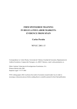
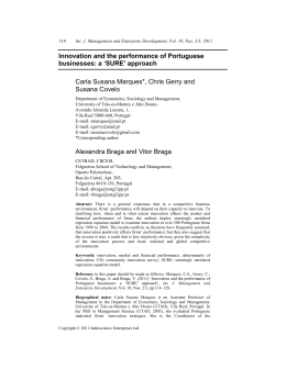
The impact of minimum wages on youth
employment in Portugal
Sonia Cecilia Pereira
Research Memorandum 0004
OCFEB
Research Centre for Economic Policy
P.O. Box 1738
3000 DR Rotterdam
The Netherlands
e-mail: [email protected]
telephone +31 10 408 2430/2446
telefax +31 10 408 9173
The impact of minimum wages on youth
employment in Portugal
1
Sonia Cecilia Pereira*
Abstract
From January 1, 1987, the legal minimum wage for workers aged 18 and 19 in Portugal
was uprated to the full adult rate, generating a 49.3% increase between 1986 and 1987
in the legal minimum wage for this age group. This shock is used as a “natural
experiment” to evaluate the impact of the minimum wage change on teenagers’
employment by using a large firm level micro-data set. It is shown that by comparing
the employment growth of 18-19 year old workers with their 20-25 year old
counterparts one can identify the employment effects of the minimum wage hike. The
same comparisons are done with 30-35 year old workers. This study finds that the rise
in the minimum wage significantly reduced employment. This conclusion is reinforced
by evidence showing that these employment effects are concentrated in firms more
likely to be affected by the change in the law.
*
Economics Department, University College London, Gower St, WC1 London.
1
I am very grateful to Stephen Machin and Jonathan Thomas for their encouragement and
stimulating guidance. I am also grateful to seminar participants at the University College
London, Sociedade Portuguesa de Investigadores em Economia 1998 Conference,
European Society of Population Economics 1999 conference, European Economic
Association 1999 conference, and International Institute of Public Finance 1999
conference. Thanks are also due to the Statistics Department of the Ministry of
Qualification and Employment and in particular to Luís Silva for excellent work in data
collection, to Eduarda Ribeiro and Miguel Gouveia for fruitful discussions, and to
PRAXIS XXI Programme for financial support.
I would like to express my deep gratitude to Idalina, Fernando, Luís, Maria, Fernanda and
Alfredo for their unconditional support.
Corresponding author, Email: [email protected]
JEL classification: J23; J30.
Keywords: Minimum wages; Youth employment; Natural Experiment
Table of Contents
Abstract .......................................................................................................................... 2
Foreword ........................................................................................................................ 4
1. Introduction ............................................................................................................... 6
2. “The Quasi-Experiment” .......................................................................................... 8
3. The data.................................................................................................................... 11
4. Minimum wages and wage changes ....................................................................... 12
5. Difference in differences: estimates of employment effects.................................. 19
6. Difference in differences: second experimental design......................................... 25
7. Firms’ entries and exits ........................................................................................... 28
8. Conclusion ................................................................................................................ 33
References .................................................................................................................... 34
Appendix I.................................................................................................................... 37
Appendix II .................................................................................................................. 40
Appendix III................................................................................................................. 42
Foreword
One of the most challenging and at the same time still controversial topics in labor
economics is the effect of the minimum wage on labor market outcomes. This research
memorandum was presented at a workshop organized by OCFEB and the Tinbergen
Institute in April 2000. The focus was on recent developments in the analysis of the
minimum wage. A mix of theory and empirical papers were presented at this workshop.
The theory papers show that frictionless Walrasian models are not able to explain the
stylized facts. Instead, we need modern economic theories which deal with imperfect
information and other market imperfections to derive novel insights into these effects.
The empirical papers show how a careful empirical analysis can shed new lights on the
magnitudes of the effects. Below we give a short overview of all the papers that were
presented at the workshop.
The Research Memorandum 0004 by Sonia Pereira (University College London), "The
impact of minimum wages on youth employment in Portugal", is about a natural
experiment in Portugal. From January 1, 1987, the legal minimum wage for workers
aged 18 and 19 in Portugal was raised to the full adult rate, generating a 49.3% increase
between 1986 and 1987 in the legal minimum wage for this age group. This shock is
used to evaluate the impact of the minimum wage change on teenagers' employment.
Her conclusion is that the rise in the minimum wage significantly reduced employment.
The Research Memorandum 0005 of Chris Flinn (New York University), "Interpreting
minimum wage effects on wage distributions: a cautionary tale", argues that welfare
effects of minimum wage effects can only be drawn by using empirical evidence on
employment changes, the wage distribution and a formal model in which welfare can be
defined in a meaningful and rigorous way. Flinn shows that negative employment
effects by itself do not tell us much about the aggregate welfare effects of the minimum
wage.
The Research Memorandum 0006 of Francis Kramarz and Thomas Philippon
(University of Paris I, CREST, and MIT respectively), "The impact of differential
payroll tax subsidies on minimum wage employment", uses changes in compensation
costs and minimum wages, to get observations of up- and down- variation in real
minimum wages. They get up-and down-movements in minimum wages in the US, with
differentiation by state, and in France an equivalent-minimum is defined, which
normalizes on the compensation cost in a base year and looks at variations in the
underlying minimum and payroll taxes to get up- and down-variation in the equivalent
minimum in France. They find no significant effects in the United States but strong and
significant effects in France.
In the Research Memorandum 0007 by Pieter Gautier and Coen Teulings (Erasmus
University Rotterdam, Tinbergen Institute, OCFEB), "A large piece of a small pie:
minimum wages and unemployment benefits in an assignment model with search
4
frictions", an assignment model with search frictions is offered that is consistent with
the following stylized facts: a spike at the minimum wage, compression of wage
differentials at a large interval above the minimum wage and small employment losses.
The introduction of a minimum wage in their model makes some matches at the lower
segments no longer profitable. In addition it leads to a redistribution of rents from firms
to low skilled workers. A minimum wage fulfills a potential useful role in this model in
the sense that it prevents low skilled workers from accepting jobs for which they are ill
suited.
Finally, Research Memorandum 0002 by Gerard van den Berg (Free University
Amsterdam, Tinbergen Institute, CEPR, OCFEB), "Multiple equilibria and minimum
wages in labor markets with informational frictions and heterogeneous production
technologies", discusses an equilibrium search model in which imposition of a
minimum wage affects wages even though, after imposition, the lowest wage in the
market is strictly larger than the minimum wage and there is no spike, so that it seems
that the minimum wage is irrelevant. The minimum wage effects are a consequence of
the fact that the model has multiple equilibria. This, in turn, is because the reservation
wage of the unemployed and the lowest production technology in use affect each other.
He shows that multiplicity is an empirically relevant phenomenon, using data from
Denmark and the United States. A minimum wage policy can be fruitfully applied to
single out the desirable equilibrium.
Gerard J. van den Berg
Pieter A. Gautier
5
1. Introduction
This paper evaluates the employment impact of the abolishment of minimum wage
st
reductions for teenagers that took place in Portugal on the 1 of January 1987. With this
minimum wage policy, workers aged 18 and 19 became entitled the full adult rate,
instead of the previous 75%. This represented a 49.3% increase between 1986 and 1987
in the legal minimum wage for this age group. This large change in the minimum wage
of a particular group of workers offers very good conditions for a “natural experiment”
in which employment variations of 18 and 19 year olds (treatment group) can be
compared with those of older workers (control groups).
This methodology is not new in evaluating the impact of minimum wages (MW) on
employment. Early studies on MW by Richard Lester (1946) and others used “natural
experiments” to study the effect of the introduction of the federal minimum wage in the
US. This approach has been revived by Card (1992a), Card and Krueger (1994) using
MW cross state variations in the US and by Card (1992b), Katz and Krueger (1992) and
Schmitt and Bernstein (1997) to look at the effect of changes in the US federal law.
Given the nature of the problem, the “natural experiment” approach has a clear
advantage over other most common methodologies: it makes use of a large exogenous
variation in the minimum wage. In fact, very often, MW do not vary much over time or
across regions or groups of workers. Adding to the fact that both in time-series and
cross-section studies the measures of MW variation mostly used are the ratio of MW
over average wage and the Kaitz index (H. Kaitz, 1970), these studies face the problem
of using a variable of interest exhibiting relatively little variation and in which most of
that variation may not come from the minimum wage itself. Moreover, the minimum
wage variation may be endogenous, as it depends on political decisions and the timing
and extent of any change may be correlated with employment expectations. This has the
potential to seriously bias employment effect estimates.
The problem of the impact of minimum wages on employment is of particular
importance given the intense debate that is taking place both on the empirical and on the
theoretical grounds. In fact, the existing evidence fails to give a clear-cut answer about
the employment effects of minimum wage policies. In Brown, Gilroy and Kohen’
survey (1982) they concluded (mainly based on time-series studies using US data before
the 1980s) that a 10% increase in the minimum wage reduces teenage employment by 1
to 3%, though with no identifiable effect on the adult labour market. This apparent
consensus has been challenged by subsequent research well represented in Card and
Krueger (1995). By using different datasets and methodologies as well as reinterpreting
and re-examining previous studies they concluded that “the new evidence points
towards a positive effect of the minimum wage on employment; most shows no effect at
all” (page1).
6
However, their work has been strongly criticised (see the reviews of Card and Krueger
in the Industrial and Labor Relations Review, 1995; papers on the minimum wage in the
American Economic Review, 1995; Neumark and Washer, 1995; Schmitt and Bernstein,
1997) and has been followed by a resurgence of work on this topic.
The most recent studies using new datasets and methodologies have failed to reconcile
the existing conflicting results. The OECD Employment Outlook for 1998 has an
assessment of the literature on this topic and states: “while differences in methodology
may account for some of the widely differing results which have emerged, it is more
difficult to reconcile the contradictory results which have arisen even when similar data
and estimation techniques have been used” (page 45).
There are nevertheless two hypotheses that seem to be supported by existing evidence.
First, if there is in fact a negative employment effect this is stronger among youths
(Brown et al., 1982, Dolado et al., 1996, Abowd et al., 1997, OECD Employment
Outlook, 1998). Second, employment effects of minimum wage changes may depend
strongly on the particular context in which they are implemented, namely the ratio of
minimum wage to average wages, the share of workers paid at the minimum, the point
in the economic cycle.
This is why it is of particular interest to evaluate the employment impact of the big
minimum wage shock that took place in Portugal in the mid 80s that was aimed directly
at teenagers: if it exists anywhere, this is the kind of situation where one can expect to
observe a rather strong employment effect. In the period from 1984 to 1986 the average
ratio of minimum wages to average wages in Portugal was still 56%. In the US this ratio
was already below 50% during the 70’s, and went well below 40% during the 80s.
(Source: OECD, Minimum Wage database). Moreover, the share of workers under 20
paid close to the minimum in that period is considerably high (see section 4 below). A
third reason for a potentially strong negative employment impact is the fact that
Portugal is a small open economy with little possibility of adjusting to such a shock via
product price increases. In fact, not only Portugal was already part of the European
Union but also the secondary sector had still strong importance when compared to the
services sector. It is well known that in general only services have any chance of
insulating from international competition.
The existence of an administrative dataset covering the universe of the Portuguese firms
makes it possible to use a highly representative sample of firms for Portugal. Also, the
results will prove robust to using different identification assumptions and specifications.
Namely the crucial hypothesis that the employment of the different age groups would
evolve similarly if there has not been the MW change will be tested.
This study concludes that in Portugal the impact of eliminating MW reductions for
teenagers was rather harmful for teenagers’ employment. The estimated elasticity is
between –0.2 and –0.4 for teenagers. From what has been said, these values are
7
unsurprisingly at the top of the range (in absolute terms) of values usually found in the
literature. Moreover, what is at stake is the impact of an extremely large change in the
MW (35.5% in real terms)2. There is also evidence of some substitution towards older
workers, ie, young adults’ employment seems to have risen slightly with this MW
policy.
The structure of this paper is as follows: the next section summarises the institutional
aspects of minimum wages in Portugal, namely the conditions under which the change
in the law took place. Section 3 describes the dataset used. Section 4 inspects the wage
distributions of the various age groups of workers before and after the MW change.
Section 5 presents the difference in differences analysis which is extended by using
firms as control groups in section 6 and by including firm entrants and exitors in section
7. Section 8 concludes.
2. “The Quasi-Experiment”
Statutory minimum wages were introduced in Portugal in 1974 following the
democratic revolution in the same year. Nowadays called RMMG (Remuneração
Mínima Mensal Garantida), MW have undergone several transformations over the
years3. This study uses a particular change that took place in January of 1987. Up to that
date, the total amount of RMMG was due to workers at least 20 years old. Workers
aged 18 and 19 years old were entitled 75% of RMMG. From then onwards, the latter
were entitled the complete RMMG4.
Changes in RMMG levels were then expected to occur every January, as since 1983 this
had been the common practice5. They would be published in the press, as soon as they
2
3
4
5
8
Given the particular setting of this study, its results are not too dissimilar from the
existing literature for Portugal. Ribeiro (1993) and Pimentel (1995) regressed
employment to population ratios against several MW measures and found elasticities
close to zero for adults and elasticities around –0.1 for male teenagers and male young
adults. Female teenagers and female young adults seemed to have much higher
elasticities of -0.2 and -0.47.
A detailed description of the Portuguese minimum wage institutional setting and
historical evolution is given in the appendix I.
Some exceptions were allowed: for handicapped workers reductions for up to 50%, for
apprentices 20% reductions for no more than two years and only in exceptional
circumstances. Finally, firms with less than 5 workers could pay the agricultural RMMG
(88% of the nonagricultural RMMG in 1987). This was already possible since the late
70’s, although the bureaucratic process was made simpler in 1987. Still, these small firms
were now required to pay the full agricultural minimum wages to workers aged 18 or
more and not 20 or more as before.
The minimum wage levels were revised on a year basis to take into account the evolution
of inflation and average wages.
were approved by the parliament in December. In particular, the new law in which we
are focusing was publicly discussed during December of 1986, and was announced in
the daily papers on the last day of that year, to be applicable from the first of January
1987.
This study will look at the short and medium term impact of this change. In order to do
that, it uses a five year panel of firms since 1985 to 1989. The information in each wave
refers to the month of March. Being so, 1986 corresponds to the situation 9 months
before the change and 1987 refers to 3 months later. However, by using data from 1985,
1988 and 1989 it will possible to evaluate the immediate as well as the medium term
impacts. 1985 and 1986 waves will be considered as qualified to represent the state of
art before the experiment, while the remaining years will be considered as having
occurred after the change in the RMMG. The time elapsed between March 1986 and the
change in the law is long enough to ensure that no anticipated adjustments were made.
In fact, August 1986 is the first time that there was any news in the Portuguese papers
about a claim to change the starting age for being entitled the full RMMG.
The analysis will be mostly centred on the periods 1986 and 1988. Using these two
years corresponds to using information of 9 months before the change and 15 months
after the change. From the several alternative combinations of years, this is by far the
one considered the most adequate. 1987 allows for only 3 months of adjustment, and it
is well known that replacing the workforce has adjustment costs of hiring and firing that
translate into time lags. By using 1989 one uses as means of comparison the
employment situation 27 months after the change in the law. It is perhaps too naive to
believe that the ceteris paribus condition that will be required for this study will hold
for such a long period.
Turning now to the methodology used in this work, the basic idea underlying a “Natural
experiment” is the same as the one of the experimental method, at the core of natural
sciences’ empirical research. The latter consists of randomising a representative sample
of “individuals” in two groups, the treatment group and the control group, maintaining
both groups under similar conditions except that one receives the treatment and the
other does not. The impact of the treatment is given by the difference between the two
groups’ outcomes.
As long as the samples are large, the fact that the two groups were randomly generated
gives no reason to believe that in the absence of the experiment the treatment group
should behave differently from the control group. Put another way the control group
provides the counterfactual for what would have happened to the treatment group, had it
not received the treatment.
“Natural experiments” like the method just described, examine the measured outcome
of a relevant variable in treatment groups and comparison groups. However, these
groups are not randomly assigned. Instead, they are in most cases the result of policy
9
changes (they can also be generated by government randomisation). As opposed to an
ideal experiment, one cannot control for the changes one is using as a source of
variation. They can however create conditions for a “natural experiment” as long as they
generate transparent exogenous variation in the explanatory variables that determine the
treatment assignment” (Meyer, 1995).
In practice, a first requirement for a “natural experiment” is the occurrence of an
exogenous shock that should be at once unanticipated and large. As has already been
said, the shock we are concerned with was clearly unanticipated. It was also an
exogenous shock. The logic behind the new law had to do with legal rights and
citizenship and not with employment concerns. In the past, for legal matters an
individual was considered an adult at 21. During the eighties it had been already
established that 18 years old was the age at which an individual was entitled to full
rights and duties in the legal system. This law generalised this principle to the statutory
minimum wage. One could argue that the timing of the decision may have been related
with the positive trends in the economy and in particular in the labour market during the
period. In any case, that will be taken into account for external validity considerations6.
Finally, the minimum wage change was remarkably large. Between December 1986 and
January 1987, the younger workers saw their MW increased by 49.3%, while workers
aged 20 or more experienced an increase in their MW of only 12%. The corresponding
percent increases in real terms are 35.5% for the former group and 1.6% for the latter
one.
In this case the “quasi experiment” evaluates the employment impact on workers aged
18 and 19 years old by making use of the unexpected and large variation in the MW for
this particular range of young workers. The two control groups consist of two older
groups of workers in the same firm, namely those aged 20 to 25 (young adults) and 30
to 35 years old (older adults). The treatment group, i.e., those aged 18 and 19, will be
referred to as teenagers in the rest of the paper. Teenagers will experience an exogenous
percent increase of the applicable real MW that exceeds the one of the control groups by
33.9 points.
To avoid relying solely on age groups as control groups and as a means to test their
adequacy as controls, the analysis will be extended by grouping firms according to their
likelihood of being affected by the new law. In particular if there is an employment
effect resulting from the MW increase, this should be stronger among firms that were
previously taking advantage of the possibility of paying lower wages to their teenagers
than in the remaining firms.
6
10
Meyer (1995) divides the conditions for validity of a “natural experiment” into the ones
that ensure internal validity – whether valid inference can be drawn from the particular
“natural experiment” – and external validity – to which extent the conclusions can be
generalized.
Given the fact that the available data is aggregated at the age group and firm levels, it is
hard to determine precisely which firms were most likely to be affected. Perfect
information could only be gathered if one knew how many workers were being paid
wages below the adults’ minimum and by how much. As there are workers not covered
by the MW law, either because their apprenticeship status or because of noncompliance, it was established that firms most likely to suffer an impact from the
abolishment of the teenagers MW reduction were those that in 1986 were paying their
18 and 19 year old workers average monthly wages at or above the MW due to this
workers, but below the adults’ statutory MW7.
In practice the difference between the employment variation of teenagers minus the
employment variation of older workers in firms considered more likely to be directly
affected by the new minimum will be compared with similar variables in firms less
likely to be directly affected by the new legislation.
3. The data
The data used in this work was computed from an extensive data source, Quadros de
Pessoal (QP), produced by the DEMQE (Statistics Department of the Ministry of
Qualification and Employment). All firms established in Portugal (Azores and Madeira
Islands are included) with paid workers are legally required to report to this database.
Being so, very small firms with only self employed people or family workers are not
accounted for. A thorough evaluation of the coverage of QP through the comparison
with Census data reveals that QP covers more workers than the Census itself, despite
the fact that very small firms are underrepresented8.
The data is gathered annually and refers to the situation of firms and workers in March
of each year (for the years under analysis). A random sample was drawn to obtain 30
per cent of the Portuguese firms in19869. The panel was then constructed by following
these firms from 1985 to 1989.
In order to maintain the representativeness of the sample for the period 1986 to 1988, a
random sample was drawn of 30 percent of the firms that started activity in 1987, and
these firms were followed until 1988. Similarly, a random sample was drawn of 30
percent of the firms that started activity in 1988. This panel gives track of the firms
which died between 1986 and 1987, as they are in the survey in 1986 but are not present
7
8
9
For obvious reasons, this criterion is likely to suffer from measurement error of different
sources. First because of the average effect mentioned, then because it assumes that
workers paid monthly wages in this range work full time and finally also because there is
nothing ensuring that these firms will not change the status of their young workers in
order not to increase wages, or that they will comply with the law.
This comparison has been done by Cardoso, 1997.
30% of the population corresponded to 32031 firms in 1986. See Table 1 in annex.
11
in the following years. Firms that died between 1987 and 1988 can be identified
likewise10. This study will also use a random sample of the firms born in 1986 by
selecting those that did not exist yet in 1985. Finally, for the analysis with firms’ entries
and exits, a random sample of 30% of the firms that died from 1985 to 1986 was also
collected.
Firm level data was gathered for three age groups. The treatment group comprises
workers aged 18 and 19 years old. The control groups were those aged between twenty
and twenty-five and between thirty and thirty-five, all closed intervals. For each of these
groups the following variables were collected: the total number of workers with ages in
that interval employed by the firm (in the payroll of the firm), average monthly hours
and overtime hours worked per individual, same for overtime hours, total wages for
normal hours and total wages for overtime. The following set of firm characteristics11
was also collected: size, district and industry. Size is the number of workers that have
worked or provided any service as self employed for the firm during March of that year.
Contrary to the age groups employment variables, which just include those workers in
the payroll of the firm, size comprises temporary contracts as well as long-term
contracts and self-employed workers providing services to the firm. The regional index
at the distrito level divides Inland Portugal in 18 area locations. They were re-ordered
into 7 larger regions believed to give a good picture of the economic regional
differences across the country12. Firms’ economic activity classification (CAE 6Digit)
was rearranged into 18 broader groups, defined according to National Institute of
Statistics (INE) criteria.
For the purpose of the present study firms located in the islands were dropped, as they
have regional governments, with autonomous policies. Public administration firms were
also excluded, for their employment policies are probably in many respects insulated
from market considerations, and I am primarily concerned with what happens to the
private economy. Finally, firms belonging to the primary sector or whose economic
activity is domestic work were dropped as they have specific minimum wage regimes.
4. Minimum wages and wage changes
The occurrence of an exogenous shock that is at once unanticipated and large may not
be enough for a valid “experiment”. In fact, a policy change may fail to have a real
10
11
12
12
Firms were considered dead if they were not in the survey in the next two following
years.
For the panel, this information refers to the year of 1986, for entries and exits, refers to
the relevant years. Date of creation of the firm was not available in the survey in those
years, and other financial and ownership indicators were information not disclosed
because of confidentiality concerns.
The country is partitioned into Northern Coastal region, Northern Inland region, Central
Coastal region, Central Inland region, Lisbon and Tagus Valley, Alentejo and Algarve.
impact on the restrictions faced by the economic agents. Being so, the first requirement
for internal validity of this “quasi-experiment” is that there is actually a treatment
group, i.e., the impact of the change in the minimum wage of workers aged 18 and 19
on their wage distribution is much heavier than the one of the new MW value for older
workers.
The wage distributions of the various groups of workers confirm that this is indeed the
case. Figure 1 depicts the wage distributions for the 3 age groups in 1986 and 198713.
For the workers aged 18 and 19 (figure 1a) there are two spikes in 1986: one at the
interval 16-18 and the other one at the interval 22-24 thousand escudos. The former
corresponds to the minimum wage enforced by law with respect to this age level
employees (16875 escudos)14. The latter corresponds to the general compulsory
minimum wage for non-agricultural workers aged 20 or older (22500 escudos). The
second spike is larger than the first: 15% of the workers lie in the 16-18 interval, while
20% lie in the 22-24 interval. This indicates that the particular minimum wage for 18-19
year old workers imposes a binding restriction on their wage distribution, although part
of these workers are already paid at least the full MW.
13
14
These wage distributions have some inprecisions introduced by the inclusion of part time
workers. As what is depicted is the monthly wage, the relationship between these
workers’ wages and the minimum wage is lost. Not all workers with wages below the 1819 year old minimum need to be part timers, however. There are partial minimum wage
exemptions for handicapped , apprentices and very small firms.
This value is obtained by: 22500x0.75.
13
Fig. 1 (a-c). Wage distributions in 1986 and 1987. (a) 18-19 year old workers; (b) 20-25
year old workers; (c) 30-35 year old workers.
Number of workers
20000
15000
1986
10000
1987
5000
60
50
40
36
32
28
24
20
16
12
8
0
0
Thousand escudos
(a)
Number of workers
60000
50000
40000
1986
30000
1987
20000
10000
60
50
40
36
32
28
24
20
16
12
8
0
0
Thousand escudos
(b)
Number of workers
30000
25000
20000
1986
15000
1987
10000
5000
Thousand escudos
(c)
Source: Quadros de pessoal, DEMQE.
14
60
50
40
36
32
28
24
20
16
12
8
0
0
In 1987 however, a very sharp spike can be observed at the 24-26 interval, which
encloses the new minimum (25200). Twenty nine percent of the workers will receive
wages within this interval15. It is worth noting that for workers receiving 16875 escudos
in 1986 and the new minimum in 1987 (25200 escudos) the jump in the minimum wage
is huge (49.3%). These 49.3% correspond to a 35.5% increase in real terms.
Looking at the wage distributions for the 20-25 years old workers (figure 1b) it is clear
that the compulsory minimum wage cuts the wage distribution in 1986, so that there are
no doubts that it is imposing a binding restriction on these workers’ wages. In 1987
however, the renewed statutory minimum seems to have lost most of its bite. In fact,
while in 1986, 23% of 20 to 25 year old workers had wages in the 22-24 interval, in
1987 only 17% had wages between 24 and 26 thousand escudos. The wage distribution
seems to have moved up independently of the minimum wage change. Note that the
change in the value of the statutory minimum for these workers corresponded to no
more than 1.6% increase in real wages.
Figure 1c displays the evolution of 30-35 year old workers wage distributions. Again,
the statutory minimum wage seems to have been more restrictive in 1986 than in 1987.
The wage distribution was sharply cut at the 22-24 interval in 1986, although many
workers were already receiving wages in the interval immediately after. In 1987, the
number of workers at the statutory minimum interval falls quite dramatically, and one
can observe a fairly even distribution with peaks at round numbers (30 and 40 thousand
escudos).
From a simple observation of the relevant age groups’ wage distributions, it is possible
to conclude that the shock in the statutory minimum applied to those aged 18 and 19
years has had a clear impact on the wage distributions of these workers. Moreover the
new value of the minimum wage for adults failed to maintain its importance in terms of
representing an active restriction on low wages. In fact, the new minimum hardly
compensated for price increases and fell behind average wages.
The same conclusion is drawn if one uses the wage data available in the sample. The
average proportional wage change of each of the 3 age groups of workers is compared
with the one of the remaining groups. The formulation used is similar to the one of
difference in differences regressions, carefully explained ahead, in section 5. Basically,
the proportional wage variation between the year before the change and the year after
the change in the MW is computed for each age group. This measure is then compared
for every combination of two age groups, so that one can check whether the average
wage of the treatment group (those aged 18 and 19) has had a sizeable proportional
increase relatively to the control groups. The relative wage changes between the two
control groups will also be compared.
15
20000 out of 63578 workers are at the interval close the minimum wage. Note that 25200
is not in the beginning of the interval, as it was with the previous values
15
The equation estimated is the following:
∆Wijt = α + βd i + γXijt + ε ijt
∆Wijt = (Wijt
where
t =1
− Wijt
t =0
) Wijt t =0 ,
(1)
is the proportional change in the
hourly real wage
of workers of age group i in firm j between time t=0 (before the treatment) and time t=1
(after the treatment). j=1,2,3.....,J, where J is the number of firms in the sample. Xijt is
a vector of the characteristics of the units under study at time t (before the treatment).
Given the data available, in the present study this vector only has variables that change
across firms so that Xijt= Xjt. The dummy variable di is 1 for observations belonging to
the treatment group and 0 for observations belonging to the control group (when
comparing the two control groups, di is 1 for the younger group).
β is the parameter of interest and captures the difference between the proportional
change in the treatment group’s average real hourly wage and the proportional change
in the control group’s average real hourly wage16. The β estimated corresponds to the
difference in differences estimator which is given by:
β DD
=
∆Wijt
i=1
-
∆Wijt
i=0
,
the difference between the time differences of the
sample means of the treatment and the control group.
As the new law was enforced from January 1987, the average wage of the treatment
group is expected to rise markedly between 1986 and 1987 (the survey data refers to
March of each year). In this way, in the period before the treatment (March 1986) the
new law was completely unforeseeable, while in t=1 (March 1987) 3 months had
elapsed since the new statutory MW, time enough to adjust wages, before major
adjustments in employment levels. Note that although this study is perhaps focusing on
the most flexible part of the workforce, the Portuguese labour market is known for
being rather rigid in terms of employment, and considerably flexible in terms of wages.
(Cardoso, 1997).
16
16
Note that this difference is computed by using firms that have workers of the relevant age
group both before and after the treatment, so that a value for the average wage is given.
For example, in a regression using the two younger groups, β gives the difference in the
average proportional wage change of the 18 and 19 year old workers in those firms that
had these young workers before and after the treatment, with the same measure for 20 to
25 year old workers in the firms that had those older workers before and after the
treatment.
The first row of table 1 shows the difference between the proportional wage17 change of
the 18 and 19 year old workers and the one of 20 to 25 year old workers. From 1986 to
1987 the very young workers had a percent wage increase that exceeded the one of
young adults by 7.2 points. If this was a general trend of those years, one would expect
that by extending the time lag to two or three years, this number would increase18.
Instead, and coherent with my claim that teenagers’ wages experienced an exogenous
shock between 1986 and 1987, the difference does not increase, on the contrary, it
amounts to no more than 5.8 points for a two year lag and 5.7 points for a 3 year lag.
The second row repeats the analysis for the older control group. Again, the proportional
wage increase of the target group is higher when just one single year interval is
considered, the one that encloses the MW change. From a percent increase 6.6 points
higher than the one of workers aged 30 to 35, this value fades away to 6 and 4.5 points
when two and three year lags are used.
It is also reassuring to observe that between the two control groups, there are no
significant differences in their percent wage changes, whatever the time interval
considered. In this way, the evidence points to a particular proportional wage increase
circumscribed to the 18 and 19 year old workers only and exactly between the two time
periods between which the MW change took place19.
17
18
19
Real hourly average wages were obtained by summing up the total monthly real wages
for normal hours with the total monthly real wages for overtime and dividing this number
by the sum of average monthly hours with overtime hours.
I actually estimated the difference between the proportional wage change for the various
combinations of groups of workers for the intervals 1987 to 1988 and 1988 to 1989.
None of the coefficients obtained was insignificantly different from zero, except the one
that compared teenagers with young adults’ proportional wages for the period 1987 to
1988. This difference was estimated to be 0.0165 (with a standard error of 0.005), and so
was very low when compared to the one of the 1986 to 1987 interval.
Similar regressions were run using as dependent variable the differences in log wages.
The results were similar to the ones of proportional wage changes. The same exercise
was done using as dependent variable difference in wage levels. In this case, one could
observe that the target group’s wages suffer a sharp rise from 86 to 87 in its average real
hourly wage level, when compared to any of the other groups, and this rise diminishes if
the time elapsed is extended. When the two control groups wages are compared the
young adults’ wages fall behind the ones of older workers, and this gap increases as time
considered is extended. This result is not surprising, as both groups have similar percent
increases in wages, which means that more experienced workers, with higher wages,
would have higher absolute variations.
17
Table 1: Differences in the proportional wage growth
Age groups pooled:
(Dummy is 1 for first group pooled)
18-19 and 20-25
18-19 and 30-35
20-25 and 30-35
1986 and 1987
1986 and 1988
1986 and 1989
0.072**
(0.005)
0.066**
(0.006)
-0.005
(0.004)
0.058**
(0.013)
0.060**
(0.013)
0.001
(0.005)
0.057**
(0.010)
0.045**
(0.011)
-0.010
(0.007)
Note: Robust standard errors in parenthesis. All regressions use as control variables the following
firms' characteristics: size, 19 industry dummies and 7 region dummies. The dependent variable is
20
the time difference in the average hourly wage.
* - Significant at 5% level., ** - Significant at 1% level.
There is enough evidence supporting the assumption that the MW change with respect
to the 18 and 19 year old workers at the centre of this study, has had a sizeable and real
impact on this workers’ wage distributions, representing therefore a binding restriction.
The two control groups exhibit similar percent wage variations which is of particular
relevance in this work. In fact, by using older workers in the firm as a control group,
one risks using spurious variation due to ripple effects. By ripple effects here I mean the
spillovers of an exogenous shock on some workers’ wages on the remaining workers’
wages. According to internal labour market theories, the structure of wages inside the
firm may be rather insulated from market wages. Jobs that are filled with workers
outside the firm are more likely to have competitive wages, while wages in jobs that are
only reached through the promotion ladder, are probably designed to provide effort
incentives, or to prevent high quit rates, leading to steeper career wage profiles. As
such, the relative position of a job’s wage on the wage structure of the firm may result
from the firm’s wage policy and the whole wage structure of the firm may change if
there is an exogenous shock on the pay of a particular group of workers. Moreover, one
would expect that the closer in the promotion ladder are the jobs to the ones that
experienced the wage change, the more likely they are to be affected. In the particular
case of this experiment, young adults’ wages are more likely to be affected by this
spillover effect than the older adults’. This could of course invalidate their use as a
control group, as they would be prone to experience similar (though probably smaller)
employment effects. This in turn would introduce a downward bias in the estimated
20
18
Number of Observations According to Groups Pooled and Years Used
Groups Pooled
1986 and 1987
1986 and 1988
1986 and 1989
18-19 and 20-25
18-19 and 30-35
20-25 and 30-35
15642
14172
20962
13386
12198
18584
12237
10982
16655
impact of MW on teenagers employment, as the methodology used is based on
comparing the outcomes in the control and treatment groups.
However, table 1 shows that the difference of teenagers wages’ percent growth seems
not to be lower with respect to the young adults group than with respect to the older
control group. This evidence goes against the possibility that the spillover effect just
described is of great importance21.
From the comparison of the proportional wage variations in the three age groups over
time, not only it was possible to gather convincing evidence of the restrictiveness of the
law change, but it also reinforced my claim that the control groups chosen are adequate,
namely, that wage spillovers are probably of minor importance.
5. Difference in differences: estimates of employment effects
The econometric analysis will be based on the straightforward difference in differences.
This is the name given to the before and after design with an untreated comparison
group. Basically, the difference between the “after treatment” outcome and the “before
treatment” outcome is computed for both the treatment and the control groups. The
difference in differences is then the difference between these two measures. This
technique has the clear advantage of differencing out all permanent individual
characteristics of each group (through the “first difference”), as well as all other shocks
or macroeconomic trends that affect both groups similarly (“second difference”). Firms’
characteristics which are time invariant are differenced out by any of the differences.
The result is the net impact of the treatment on the outcome for the treatment group.
The formulation used is the following:
21
One must keep in mind nevertheless, that similarly to other countries, a well documented
wage inequality increase took place in Portugal during the eighties, favouring skilled
workers (Cardoso, 1997). This means that the older group’s wage variations, (even if age
is not a perfect proxy for skill), may be affected by a time trend.
Given what has been said, it would still be possible that the wage estimates could suffer
from downward bias as young adults wages could be inflated due to the spillover effect,
and still the wage growth of teenagers against the one of young adults would not be much
higher than when compared to older workers as the older group’s wages growth would be
persistently higher.
Being so, the fact that the third row of table 1 comparing the wage growth of the young
adults with the one of 30 to 35 year old workers shows no evidence of statistically
significant differences, would not give unambiguous information. It could be the result of
similar wage growths with different sources: spillover effects for young adults and skill
biased wage growth for older workers. However, the fact that whatever the time lag
considered (1 to 3 years), the coefficients are persistently insignificant give no support to
such interpretation as the spillover effect should fade away, while the older group’s wage
growth should be persistent.
19
∆Yijt = α + βdi + γX jt + ε ijt
(2)
where ∆Yijt is the change in the number of workers of age group i in firm j between
time t=0 (before the treatment) and time t=1 (after the treatment). j=1,2,3.....,J, where J
is the number of firms in the sample. Xjt is a vector of the firm characteristics at time
t=0 (before the treatment). The dummy variable di is 1 for observations belonging to the
treatment group and 0 for observations belonging to the control group. β is the
parameter of interest and captures the difference between the change in the treatment
group’s average employment and the change in the control group’s average
employment. The difference in differences estimator is given by:
β DD
=
∆Yijt
i=1
-
∆Yijt
i=0
,
the difference between the time differences of the sample means of the treatment and
the control groups. The key identifying assumption of this model is that in the absence
of the treatment, the average employment change in both groups would be the same:
β DD
=0 or E
[ε d ] = 0 .
ijt
i
In practice the same regression was performed twice, one for each control group, using
as dependent variable a pool of the employment changes in the treatment and one of the
control group. As a robustness check the same regression was run for the 2 control
groups, as if one of them was a treatment group. In this case, β is expected to be
insignificantly different from zero.
The dependent variable of equation (2) will be in separate regressions, the difference in
the number of workers at specific age intervals and the difference in the total time
worked by those workers.
As the above specification implies that in each regression there are 2 observations for
each firm, the OLS standard errors are corrected by allowing nonindependence between
the two observations of the same firm. A random effects model is used which allows for
a correlation coefficient different from zero constant across firms.
With respect to the time difference, the following intervals will be investigated:
[1986;1987], [1986;1988], [1986;1989], [average 1985 and 1986; average 1988 and
1989], [average 1985 and 1986; average 1987, 1988 and 1989].
Table 2 shows the difference in differences’ coefficients for different age groups and
time periods. The dependent variable is the difference in the total number of workers in
the payroll of the firm for the age groups and time intervals considered. Each cell
corresponds to a separate regression.
The sign of the coefficients in the first two rows clearly suggests a negative impact on
the target group’s employment. For all time intervals considered, the relative
20
employment of 18-19s decreased when compared to 20-25s. Moreover, this effect
seems to have persisted up to 1989. When the older control group is used, the
coefficients are still estimated to be negative, though they only remain significant for
the difference between 1986 and 1988.
Table 2:
Impact on the Number of workers
Age groups
1986
(Dummy is 1 for 1st group) 1987
18-19 and 20-25
-0.087**
(0.020)
18-19 and 30-35
-0.025
(0.020)
20-25 and 30-35
0.063**
(0.023)
1986
1988
-0.196**
(0.033)
-0.107**
(0.033)
0.089**
(0.037)
1986
1989
-0.223**
(0.041)
-0.010
(0.056)
0.212**
(0.059)
1985/86
1988/89
-0.202**
(0.041)
-0.100
(0.062)
0.102
(0.064)
1985/86
1987-89
-0.173**
(0.036)
-0.087
(0.055)
0.086
(0.057)
Number of Firms
Number of Observations
22014
44028
20895
41790
16685
33370
15993
31986
23879
47758
Note: Robust standard errors in parenthesis. Other regressors are: size, 19 industry dummies and 7
region dummies. Region dummies are in most cases not significant, while other controls are. Firm
controls just reduce slightly standard errors, not affecting the coefficients (see appendix I). With
differences inside the firm, one should not expect these controls to change the difference in
differences estimates.
* - Significant at 5% level.
** - Significant at 1% level.
For the 1986-1988 interval the employment growth of the group affected is smaller than
the one of any of the control groups, so that there seems to be a clear negative
employment impact. On average, the teenagers employment growth per firm was 0.196
workers less than the young adults’ employment growth. Comparatively to the older
group, however, teenagers’ employment grew on average less 0.107 workers.
rd
Turning to the difference in differences with the two control groups presented in the 3
row, the group of young adults had experienced a continuous employment increase
compared to the older group of workers over the 1986-1989 period.
For the moment I will assume that the different age groups of workers do not follow
different employment trends, so that all the changes observed are due to the change in
the statutory minimum wage. That is to say that in the absence of the MW change, all
coefficients would not have been significantly different from zero.
With this assumption, the fact that the young adults had an employment boost against
any of the other groups would have been the result of a direct employment substitution
effect. I argue that employment substitution effects are likely to occur between rather
21
similar workers, in this case teenagers and young adults, and unlikely to occur between
teenagers and workers aged 30 or more22.
The employment effect given by the difference in differences between the two younger
groups would then be overestimated in absolute terms23, while the employment effect
suggested by the older control group results would be a good approximation for the true
employment effect.
nd
Focusing on the interval 1986-1988 (2 column), the third coefficient would give the
size of the substitution effect towards young adults in terms of average growth in the
number of workers. The coefficient in the first row would then have to be corrected by
deducting the substitution effect. By construction, the value obtained would be the one
nd
shown in the 2 row: –0.107, and this would measure the true MW impact. That
employment effect would correspond to a –0.4 employment-minimum wage elasticity
for 18 and 19-year-old workers. A ten percent increase in this group of workers
22
23
22
Young adults (from 20 to 25 years) in the same firm as teenagers (aged 18 and 19) are
likely to provide good controls, as they are not much different in terms of education,
experience, tenure and skills. However, as we are clearly not dealing with independent
labour markets, this will imply a large degree of substitutability between the two groups
which may in turn introduce an element of bias. In fact, once the law enforces the same
minimum wage for both groups of workers, it may be profitable to switch to the older
group, as they have an advantage in terms of education, experience and tenure, though
marginal it may be (note that wage profiles are quite steep in the begining of individuals’
carrers, one hypothesis being the rapid accumulation of human capital, Borjas, 1996).
This would imply a downward bias in the difference in differences estimates.
It has been mentioned in the previous section that the existence of wage spillovers (ripple
effects) could underestimate the employment effect generated by the difference in
differences regression between the two younger groups. I argued that these ripple effects
did not seem to be of sizeable importance. The same does not seem to be true with
respect to substitution effects. The debate will therefore be centred on the bias generated
by employment substitution effects across age groups. However, as wage spillovers
would lead to a smaller employment difference in differences between the target group
and the younger control group, they would “smooth” the substitution effect. As it is,
wage spillovers would bias the employment-minimum wage elasticity on the opposite
direction of the substitution effect. The present analysis can be seen as considering the
substitution effect from teenagers to young adults “net” of the impact of the potential
wage spillover.
statutory real minimum wage would generate a four percent decrease in this group’s
employment24.
The gross elasticity of substitution between young adults’ employment and teenagers
MW is 0.0925. So, in the present experiment a 10 percent increase in 18 and 19 year old
workers minimum wage has generated a 0.9 percent increase in the young adults’
employment, and a 4.0 percent decrease in teenagers’ employment26.
The pattern of evolution suggested by the coefficients for different time intervals does
not offer a clear-cut picture. If one looks at the results with the younger control group
the treatment group’s employment seems to fall until 1989. However, if one focus on
the older control group, it seems to fade away after 1988. Various potential reasons
could be put forwarded as to explain the dynamics of these employment effects.
In a before and after analysis however, the exact time periods chosen as period “before”
and period “after” are crucial, and I acknowledge that if one allows for long intervals,
not only is the ceteris paribus condition less likely to hold, but also spurious variation is
likely to be amplified. Being so, at this point, the analysis will be restricted to the period
considered the most adequate for the experiment.
Just as the possibility of occurrence of an employment substitution effect between
groups of workers, an “income-type effect” might as well have taken place. The firm
not only faced and exogenous change in the relative “price” of different workers, but it
also suffered an exogenous increase in the total wage bill. The impact of the MW
change on the treatment group employment that one ideally would like to estimate is the
total impact, which includes both substitution27 and income effects. It is possible,
however, that by the wage-bill effect alone the firm may reduce its whole workforce,
either homogeneously or asymmetrically across different types of workers. As all
variations that are homogeneously extended to the entire workforce will not be captured
24
25
26
27
The elasticity was calculated using the ratio given by –0.107 over 18-19 year old workers
average employment in 1986 (for the firms used in the regression: 0.785) and the percent
variation in the real minimum wage for the same group of workers, to which I subtracted
the percent change in the real MW for other workers: –0.004 = (0.107/0.785)/(35.5-1.6).
If we did not subtract the change in the real statutory MW for other workers, and simply
used the percent variation in the teenagers real minimum wage the elasticity would be –
0.38.
Calculations similar to the ones of direct elasticity: 0.0009 = (0.089/2.798)/(35.5-1.6).
Given that we are using a quasi experiment it is obviously beyond the scope of this study
trying to measure any kind of impact on the total employment.
Substitution effect is the one resulting from different relative prices for different types of
workers. Note that the income effect as it is defined, may generate a labour-capital
substitution effect
23
by the present quasi experiment, the wage-bill effect could give rise to an
underestimated employment elasticity.
Table 3 displays the coefficients for the impact on the number of hours worked by the
total workforce of the relevant age groups. The conclusions derived before are entirely
reinforced by these results. In fact, table 3 mimics table 2 in terms of both the
significance and sign of the estimated coefficients.
Using alternatively each of these two measures of labour input (number of workers and
number of hours worked) may generate different results. In fact, if there is an
employment effect, for instance, a negative one, firms may either adjust mainly through
firing and (not) hiring or may prefer to keep most of their workers and reduce their
working time, introducing more part-time positions, etc. This is especially relevant for
young workers, as there seems to be a considerable high share of part-timers, and
usually part time work is associated with more flexible contract forms.
Table 3:
Impact on the number of hours worked
Age groups pooled:
1986
(Dummy is 1 for first group) 1987
18-19 and 20-25
-17.82**
(3.53)
18-19 and 30-35
-5.22
(3.90)
20-25 and 30-35
12.60*
(4.29)
1986
1988
-46.86**
(5.82)
-29.38**
(6.36)
17.48*
(6.95)
1986
1989
-47.81**
(7.21)
-8.45
(10.45)
39.36**
(10.72)
1985/86
1988/89
-45.25**
(7.28)
-25.54*
(11.75)
19.70
(11.87)
1985/86
1987-89
-37.44**
(6.36)
-20.30*
(10.45)
17.14
(10.58)
Number of Firms
Number of Observations
22014
44028
20895
41790
16685
33370
15993
31986
23879
47758
Note: Robust standard errors in parenthesis. Other regressors are: size, 19 industry dummies and 7
region dummies.
* - Significant at 5% level.
** - Significant at 1% level.
Both adjustments (through hours worked per individual and through number of
individuals) will be captured by using hours worked as dependent variable, but one will
not be able to distinguish between them. On the other hand, when one uses changes in
the number of employed people instead, one just estimates employment adjustments
through hiring and firing.
Being so, table 3 not only provides some robustness check on the previous results, but
can also bring some additional information. It is possible to compare the coefficients in
similar positions in tables 2 and 3 by resorting to simple calculations. Table 2 showed
that between 1986 and 1988 the average growth of the number of teenagers per firm
24
was 0.196 workers lower than the growth of young adults’. These workers would have
to be working 239 hours per month to generate an average loss of 46.86 in the number
of hours if all employment adjustment had been made through hiring and firing. For the
results obtained with the older control group this number is even higher (273.5 hours a
month). As it is, there seems to be some evidence that teenagers’ average working time
suffered a reduction so that the employment impact is not completely captured by
changes in the number of people working.
6. Difference in differences: second experimental design28
The second experimental design groups firms according to their likelihood of being
affected by the MW change. If there is indeed an employment impact from the change
in the MW, then it should be larger among those firms. A firm is more likely to be
affected if the average wage paid to teenagers in 1986 is at or above the MW due to
teenagers in 1986 and below the MW for adults in 1986. A dummy variable Ai is
introduced which takes the value 1 for firms more likely to be affected by the MW
change and 0 otherwise.
The estimated regression also requires an interaction dummy variable di.Ai:
∆Yijt = α 0 + α 1 Ai + α 2 d i + βd i . Ai + γX ijt + ε ijt
(3)
The indexes i j and t have the same meaning as before. ∆Yijt is the change in the
number of workers of age group i in firm j between time t=0 (before the treatment) and
time t=1 (after the treatment). Xjt is a vector of firm controls. As before, di is 1 for
observations in the treatment age group and 0 otherwise. The parameter α1 captures the
difference in employment changes that are common to both age groups between firms
more likely to be affected and firms less likely to be affected by the MW change. α2
summarises the way in which the difference in employment change between the two age
groups is common to the two groups of firms. The parameter of interest, β tests whether
the difference in differences done before with the two age control groups is different for
firms more likely to be affected by the MW change and firms less likely to be affected
by the MW change. The identifying assumption is that if the difference between the
employment time differences of teenagers and older workers is not related with the
change in the law, then β=0. That is to say that assuming that certain firms are more
likely to be affected by the change in the law than others, then if there is a negative
impact on teenagers’ employment as suggested by the previous results, this impact
should be stronger in those firms.
28
The second experimental design tests whether the former different groups’ employment
were being driven by asymmetric omitted trends or variables. Still, the different age
groups’ employment evolution is depicted in Appendix II.
25
One can also test whether different trends may be affecting asymmetrically the control
groups’ labour markets. Suppose one could separate firms in two groups: those affected
by the MW change and those not affected. If α2=0, then all employment changes
between two age groups would only take place in firms affected by the MW change.
This would give a clear indication that the asymmetric behaviour between the control
groups was due to the spillover effects and not to the existence of omitted variables or
trends affecting the two control groups differently. In fact, the underlying assumption is
that if these asymmetries arise because of omitted variables or trends unrelated with the
MW change, then they should occur homogeneously across both types of firms.
Table 4:
Impact on the Number of workers using firms as control group
Dependent variable: difference in number of workers between:
age groups: 18-19 and 20-25
age groups: 18-19 and 30-35
1986
1986
1986
1986
1986
1986
Dummy variables:
1987
1988
1989
1987
1988
1989
di (1 if teenagers)
0.020
-0.035 -0.073
0.025
-0.011 0.090
(0.020) (0.033) (0.042)
(0.022) (0.036) (0.063)
Ai
0.434** 0.585** 0.377*
-0.004
0.134
0.146
(0.090) (0.139) (0.183)
(0.067) (0.106) (0.174)
di. Ai
-0.886** -1.278** -1.196**
-0.411** -0.762** -0.803**
(0.081) (0.121) (0.143)
(0.062) (0.089) (0.114)
Number of Firms
Number of observations
Number of observations
if Ai=1
23879
47758
5786
22014
44028
5544
20895
41790
5228
23879
47758
5786
22014
44028
5544
20895
41790
5228
Note: Robust standard errors in parenthesis. All regressions include the three dummies. Other
regressors are: size, 19 industry dummies and 7 region dummies.
* - Significant at 5% level.
** - Significant at 1% level.
Table 4 presents the results of the difference in differences when firms are used as a
control group, instead of relying solely on age group comparisons. Each column
corresponds to a separate regression. The dependent variable is the difference in the
number of workers between the relevant years for two of the age groups (as before, the
two groups are pooled).
The coefficients are shown for the dummy variables. Again, the results point to a
negative employment effect. Only di.Ai has a significant negative coefficient for all
time intervals and for any of the two age groups. The fact that the di coefficient is
persistently not significant seems to indicate that the previous estimated employment
impact which compared two age groups’ employment variation is not a general problem
being instead concentrated in those firms most affected by the new MW. Given these
results, it seems rather unlikely that the initial estimations could have been seriously
26
biased by possible exogenous trends affecting asymmetrically the various age groups’
employment.
With this formulation it is now possible to decompose the difference in differences
estimated before in two parts. The first one is the one that takes place in firms less likely
to suffer the MW impact and the other one is the one that takes place in firms more
likely to suffer the MW impact. The total difference between two age groups’
employment change will be given by a weighted average of this two parts, where the
employment changes in the two groups of firms is weighted by the proportion of firms
belonging to each of the groups:
β DD = ∆Yijt
=α2
i=1
- ∆Yijt
i=0
=
n1
n2
+ (β + α 2 ) where n1 is the number of firms less likely to
n
n
be affected by the MW change, n is the total number of firms and n2=n-n1.
Table 5 gives the average employment effects in the two groups of firms using the
results from table 4. The last row is a weighted average of the two previous rows in
which the weights are the proportion of firms (or observations) belonging to the relevant
groups. As expected, these numbers are exactly the same as the ones displayed in table
2.
Table 5:
Net employment effects
Employment difference in differences between:
18-19 and 20 –25
18-19 and 30-35
1986
1986
1986
1986
1986 1986
Group of Firms
1987
1988
1989
1987
1988 1989
A1=1 (β+α2)
-0.866 -1.313 -1.269 -0.386 -0.773 -0.713
A1=0 (α2)
0,020 -0,035 -0,073 0,025 -0,011 0,090
weighted average -0.087 -0.196 -0.223 -0.025 -0.107 -0.010
20-25 and 30-35
1986 1986 1986
1987 1988 1989
0.480 0.540 0.556
0.005 0.024 0.163
0.063 0.089 0.212
Table 5 provides us with rather interesting results. Firstly, the first 6 coefficients of the
first row confirm that the bulk of the negative impact on teenagers’ employment takes
place mostly in the firms considered more likely to suffer with the change in the law.
Secondly, the last 3 coefficients of the first row indicate that the increase in the
employment of young adults with respect to older adults also seems to be concentrated
in the same group of firms. This gives strong support for the initial hypothesis of a
substitution effect towards young adults.
Finally, from the employment difference in differences between teenagers and older
adults, the relative employment fall of the former is observable up to 1989, as it is when
comparisons are made with the younger control group. The “fade away” phenomenon
27
observed in the initial results occurs only in firms less likely to be affected by the MW
change. This phenomenon is therefore probably driven by some omitted variable
changing between 1988 and 1989, which is affecting the employment of young adults
and is unrelated with the minimum wage change.
7. Firms’ entries and exits
The fact that difference in differences is entirely based on firms that were observed
before and after the change in the law may be a source of possible bias. In fact, by
excluding from the analysis firms that died or were born after 1986 one risks to miss
part of the picture of the employment evolution of the different age groups. New firms
are very likely to absorb a disproportionately high share of younger workers, as there
are no tenure gains associated with its workforce. Moreover, as it can be observed in
table 2 in the appendix, entry and exit of firms is an important phenomenon in the
Portuguese economy. Adding to that the simple fact that the working population inside
the firms belonging to the panel is likely to get older, one has reasons to believe that the
previous estimates were downward biased29.
As an attempt to deal with the problem just mentioned, the previous analysis will be
extended to a representative sample of firms before the treatment and the outcomes will
be compared with the ones of a representative sample after the treatment. The difference
in differences has been defined as:
β DD
=
∆Yijt
β DD
=
Yijt
i=1
i =1,t =1
-
∆Yijt
-
Yijt
i= 0
, which is the same as:
i = 0 ,t =1
- [ Yijt
i =1,t = 0
-
Yijt
i = 0 ,t = 0
],
where the first difference is taken between groups in the same time period and only then
time differences are taken between these two measures.
The same measure is now calculated using representative samples for t=0 and t=1. The
period t=0 corresponds to the year of 1986 and the sample randomly selected includes
firms remaining in subsequent years, which are the ones used so far in difference in
29
28
Further problems arise when omitting entrants and exitors from the analysis. In particular
there may be an attrition bias as firms’ destruction may not be an exogenous
phenomenon. Firms may face unbearable wage pressure arising from the new minimum
wage which forces them to shut down. In this case difference in differences would give
upward biased estimates. Similarly, firms’ creation may be endogenous. There may be
less new firms after 1986 than otherwise would have been without the wage change.
Unfortunately, it will not be possible to correct for these biases as there is no suitable
instrumental variable to provide identifying restrictions to model attrition.
differences, but also includes firms that will die after the treatment, exitors. The sample
used for t=1 is made of the firms that survive until t=1 (in our study, t=1 will correspond
to 1987 and 1988 in separate regressions) together with all the firms that were born
meanwhile.
Now the difference in differences estimator for the representative sample is:
βˆ EED = Y ijtP
i =1,t =1
− Y ijtP
− Y ijtP
{
i =1,t = 0
− Y ijtP
i = 0 ,t =1
+ Y ijtIN
+ Y OUT
ijt
i = 0 ,t = 0
i =1,t =1
i =1,t = 0
− Y ijtIN
− Y OUT
ijt
i = 0 ,t =1
i = 0 ,t = 0
−
}
In practice zeros are given to exitors’ employment of any age group in t=1, and to
entrants’ similar variables in t=0 and regressions similar to (1) and (2) are estimated.
With this “difference in differences”, permanent group (treatment and control groups)
characteristics are still differenced out by taking differences between entrants and exitors
(Y
IN
ijt i =1,t =1
− YijtOUT
i =1,t = 0
)
. The same is true for macroeconomic trends that affect
both groups similarly:
( y ijtIN
i =1,t =1
− y ijtOUT
i =1,t = 0
) − ( y ijtIN
i = 0 ,t =1
− y ijtOUT
i = 0 ,t = 0
Also permanent firm characteristics are differenced out
)
(Y
IN
ijt i =1,t =1
− YijtIN
i = 0 ,t = 0
)
.
However, the impact of variables that are both firm and group specific is not eliminated,
as for entrants and exitors this method fails to take differences between two periods for
the same group of workers inside each firm. Finally, if the number of entrants and
exitors is not balanced, then group specific variables are not completely differenced out
and additional spurious variation is introduced. In both time intervals considered there
was a higher number of new firms being created than firms shutting down. As firms
entering the market have on average more workers of any of the older age groups than
workers in the treatment group, their contribution to the difference in differences
estimator has a negative sign. In this case, not differencing out group specific variables
would result in a negative bias in the difference in differences coefficient.
As a robustness check, a 2-step methodology is used to proxy the “missing employment
values” in the representative samples. The basic idea is to produce a counterfactual for
what would have been the various age groups’ employment of an entrant or an exitor if
it could have existed as such before the treatment.
The two-step procedure makes use of two samples of firms, one with firms which exit
the market between 1985 and 1986 and the other with firms born in 1986. For each of
these samples the employment of each of the age groups is regressed on a set of firm
characteristics. The predicted values are then used to compute the employment levels,
29
used in the difference in differences for entrants and exitors. This alternative way of
obtaining employment values for the “blank years” reduces the impact of unobserved
variables that are both firm and group specific as well as the effect of group specific
variables coming from the difference in the number of entrants and exitors.
In both methods of proxying the employment differences for entrants and exitors, a
similar equation to the previous ones is estimated:
∆Yijt = α 0 + βˆ RDD d i + γX ijt + ε ijt
(4)
where βˆ RDD gives the difference in differences for the representative samples.
Table 6:
Impact on the Number of workers: panel of firms and representative samples’ results
compared
Age Groups
panel
representative samples
original
zeros for
2-step
results
counterfactual
procedure
1986
1986
1986
1986
1986
1986
1987
1988
1987
1988
1987
1988
18-19 and 20-25
-0.087** -0.196** -0.083** -0.204** -0.075** -0.144**
(0.020) (0.033) (0.016) (0.022) (0.016) (0.021)
18-19 and 30-35
-0.025
-0.107** 0.013
-0.036
-0.012 -0.056**
(0.020) (0.033) (0.016) (0.022) (0.016) (0.022)
20-25 and 30-35
0.063* 0.089*
0.096** 0.168** 0.063** 0.088**
(0.023) (0.037) (0.018) (0.025) (0.018) (0.025)
Number of Firms
23879
Number of Observations 47758
22014
44028
32871
65742
37461
74922
32871
65742
37461
74922
Note: Robust standard errors in parenthesis. Other regressors are: 8 size dummies, 19 industry
dummies and 7 region dummies.
* - Significant at 5% level.
** - Significant at 1% level.
Table 6 compares the results with the ones obtained when only the observations
belonging to the panel were used. The signs of all but one coefficient remain the same.
The coefficient comparing the employment growth of teenagers with the one of young
adults does not change when zeros are used for the counterfactual, but is significantly
lower in the 2-step procedure. When older adults are used as control group, while the
coefficient referring to the period between 1986 and 1987 remains insignificant across
all specifications, the one corresponding to the 1986-1988 period decreases significantly
for the representative samples.
30
As 1986-1988 is probably the right time interval to consider, this result suggests that
excluding exitors and entrants overstates the employment effects.
By estimating the following equation it is possible to have a more detailed picture of the
separate contributions of entrants and exitors to the final result:
∆Yijt = α 0 + α 1 d iIN + α 2 d IN + α 3 d iOUT + α 4 d OUT + βd i + γX ijt + ε ijt
The dummy variable d
interaction dummy di
IN
IN
(5)
takes the value 1 if the firm is an entrant and 0 otherwise. The
is 1 if the difference in employment refers to the control group
of an entrant and 0 otherwise. di
OUT
and d
OUT
are similar dummy variables for exitors.
The parameters α2 and α4 capture the extent to which entrants and exitors’ average
employment changes of both age groups are different from the remaining firms. The
coefficients α1 and α3 summarise the way in which the difference in employment
change between the two groups among entrants and exitors is dissimilar to the one of
firms in the panel. β captures the MW impact on the treatment group employment in the
panel of firms as the different impacts of entrants and exitors is picked up by the other
dummy variables. Therefore, β is the same coefficient as the one estimated in (1).
β RDD
can be decomposed as follows:
m1
m2
m3
βˆ RDD = β
+ (β + α 1 )
+ (β + α 3 )
m
m
m
where m1 is the number of firms in the panel, m2 is the number of entrants, m3 is the
number of exitors and m is the total number of firms.
Table 7 displays the decomposition of the employment impact among firms in the
panel, exitors and entrants. The coefficients in first row (panel of firms) are the same as
the ones shown before in table 2. Last row shows the difference in differences estimates
for the representative sample. When zeros are used for the counterfactual (table 7a),
exitors contribution to the relative employment of teenagers has a positive sign, while
entrants’ contribution has a negative sign. In practice this simply means that both new
firms and firms close to leaving the market employ less teenagers than any of the older
groups of workers. As the difference between teenagers’ and young adults employment
is similar for both exitors and entrants, the impact of these groups of firms cancel out.
However, if one uses older workers as control group, teenagers are outnumbered by
older workers to a much larger extent among exitors than among entrants30. This drives
30
One expects that to happen as older firms are more like to have an older workforce, for
the reasons already mentioned.
31
the coefficient corresponding to period 1986 to 1988 down from –0.107 to –0.03631. In
the 2-step procedure exitors’ contribution to the employment effect has a negative sign,
although it is less negative than the one of the panel. This implies that the average
employment difference between teenagers and any of the older groups is larger than it
was in firms that exited in 1986. Also, the coefficients corresponding to the new-born
firms is never as negative as the one of the panel.
Table 7:
Net employment effects
(a) zeros for counterfactual
Group of Firms
Panel β
Entrants (β+α1)
Exitors (β+α3)
weighted average
(b) 2-step procedure
Group of Firms
Panel β
Entrants (β+α1)
Exitors (β+α3)
weighted average
18-19 and 20-25
1986-1987 1986-1988
-0.087
-0.196
-0.706
-0.846
0.698
0.804
-0.083
-0.205
18-19 and 30-35
1986-1987 1986-1988
-0.025
-0.107
-0.160
-0.225
0.441
0.538
0.013
-0.036
18-19 and 20-25
1986-1987 1986-1988
-0.087
-0.196
0.007
-0.065
-0.101
-0.075
-0.075
-0.144
18-19 and 30-35
1986-1987 1986-1988
-0.025
-0.107
0.055
0.029
-0.021
-0.004
-0.013
-0.056
Representative sample results provide the lower boundaries for the employment impact
resulting from the teenagers minimum wage increase. Focusing on the interval between
1986 and 1988 and at the regressions using older adults as control group, the
employment elasticity32 is –0.2 when zeros are used as counterfactual and –0.26 in the
2-step methodology. Given the possibility of selective attrition, the true employment
31
32
32
One must be careful about the validity of the control groups under this circumstances.
Indeed, it is difficult to argue that the magnitude of the employment difference in
differences between 1986 and 1988 for the two adult groups, 0.168 (table 6, row 3,
column 4) is due to the substitution effect.
When zeros were given to the counterfactuals, the elasticity was calculated using the ratio
given by –0.036 over the average number of 18-19 year old workers average employment
in 1986 (because of the zeros introduced, the mean is smaller than the one in previous
calculations: 0.519) and the percent variation in the real minimum wage for the same
group of workers (35.5), to which we subtracted the percent change in the real MW for
other workers (1.6): –0. 2 = (-0.036 /0.519)/(35.5-1.6)x100. The same calculations give
the following result for the two-step methodology:
–0. 26 = (-0.056 /0.627)/(35.5-1.6)x100.
elasticity is expected to lie somewhere in the interval between –0.2 and the original
value, –0.4.
8. Conclusion
Portugal offers extraordinary conditions to evaluate the impact of Minimum Wages
(MW) on teenagers’ employment following a “quasi-experiment” analysis. First, the
change in the law in the MW of the 18 and 19 years old workers in January of 1987
proved to have had a clear binding effect on these workers’ wages. Secondly, the use of
older workers as control groups seems to have given good results. Thirdly, the
possibility of using a large dataset of microdata gives this study a comparative
advantage with respect to previous studies.
The estimated results show that the abolition of 25% of the MW reduction for teenagers
had a significant and negative impact on teenagers’ employment. This impact seems to
have persisted for more than 2 years. It was also provided evidence of a substitution
effect towards workers aged 20 to 25 years old. These results are rather robust to two
experimental designs which hinge on different assumptions. There is some indication
that employment adjustment is done both by reducing the number of teenagers
employed and the time worked by those who remain employed.
The results obtained point to an elasticity among the highest (in absolute terms) found
in the literature. The values found were in the range –0.20 to –0.40. I believe that this
might be the case because what is at stake is the impact of a very large change in the
MW, because the study focus on very young workers (expected to be among those with
lowest productivity) and also because Portugal during the 80’s had a rather high MW
average wage ratio. The economic conditions of the period are unlikely to have been
responsible for the negativity of estimated elasticity, as Portugal was experiencing a
period of economic recovery and employment expansion.
This work supports the idea that negative employment effects are probably higher
among teenagers than among adults and that some substitution effect towards workers
with higher marginal productivity is likely to occur.
33
References
Abowd, John M., F. Kramarz, T. Lemieux and D. Margolis, 1997. Minimum Wages and
Youth Employment in France and the United States. National Bureu of Economic
Research, Working Paper 6111.
Bazen, S., Skourias, N., 1997. Is There a Negative Effect of Minimum Wages on Youth
Employment in France?. European Economic Review 41, 723-732.
Belman, Dale, Wolfson, Paul, 1996. A Time Series Analysis of Employment and the
Minimum Wage. Mimeo.
Blanchard, Olivier, and Jimeno, Juan, 1995. Structural Slumps and Persistent
Unemployment - Structural Unemployment: Spain Versus Portugal. American
Economic Review 85, 212-18.
Brown, Charles, C. Gilroy and A. Kohen, 1982. The Effect of the Minimum Wage on
Employment and Unemployment. Journal of Economic Literature 10, 487-528.
Card, D., 1992a. Do minimum wages reduce employment? A case study of California,
1987-1989. Industrial and Labour Relations Review 46, 38-54.
______, 1992b. Using regional variation in wages to measure the effects of the Federal
minimum wage. Industrial and Labour Relations Review 46, 22-37.
______, 1994. Do Minimum Wages Reduce Employment? A case Study of the Fast
Food Industry in New Jersey and Pennsylvania. American Economic Review 84,
772-93.
Card, D., Katz, L., and A. Krueger, 1994. Comment on David Neumark and William
Wascher, Employment Effects of Minimum and Subminimum Wages: Panel Data
on State Minimum Wage Laws. Industrial and Labour Relations Review 47, 48797.
Card, D. and Krueger, A., 1998. A reanalyses of the effect of the New Jersey minimum
wage increase on the fast food industry with representative payroll data. National
Bureau of Economic Research, working paper 6386.
______, 1995. Myth and Measurement - The New Economics of the Minimum Wage.
(Princeton University Press, Princeton, NJ).
Cardoso, Ana Rute, 1994. Regional Wage Inequality. Mimeo.
______, 1995. Workers or Employers: Who is Shaping Wage Inaquality?. Mimeo.
______, 1997. Earnings Inequality in Portugal: the Relevance and the Dynamics of
Employer Behaviour. European University Institute, Florence. PhD Thesis.
Dickens, Richard, Machin, Stephen, Manning, Alan, Wilkinson, David, 1995. What
Happened to Wages and Employment After the Abolition of Minimum Wages in
Britain?. Mimeo.
Dickens, Richard, Manning, Alan, 1995. After Wage Councils. New Economy, 223-27.
Dolado, Juan, F. Kramarz, S. Machin, A. Manning, D. Margolis and C. Teulings, 1996.
The Economic Impact of Minimum Wages in Europe. Economic Policy, October,
319-72.
Dolado, J., Felgueroso, F., Jimeno, J., 1997. The effects of minimum bargained wages
on earnings: evidence from Spain. European Economic Review 41, 713-721.
34
Evans, W. and Turner, M., 1995. Employment Effects of Minimum and Subminimum
Wages: Comment. The Urban Institute, Washington. Mimeo.
Guimarães, P., Portugal, P., 1996. The Influence of Local Labor Market Conditions on
the Entry and Exit of Plants. Mimeo.
Kaitz, Hyman, 1970 Experience of the Past: the National Minimum, Youth
Unemployment and Minimum Wages, Bulletin 1657, U.S. Department of Labor,
Bureu Of Labor Statistics.
Katz, L. and Krueger, A., 1992. The Effect of Minimum Wage in the Fast Food
Industry. Industrial and Labour Relations Review 46, 6-21.
Lang, K. and Kahn, S., 1998. The Effect of Minimum-Wage Laws on the Distribution
of Employment: Theory and Evidence. Journal of Public Economics 69, 67-82.
Linneman, Peter, The Economic Impacts of Minimum Wage Laws: A New Look at an
Old Question. Journal of Political Economy 90, 443-69.
Machin, S. and Manning, A., 1994. The Effects of the Minimum Wages on Wage
Dispersion and Employment: Evidence from the U. K. Wages Councils. Industrial
and Labour Relations Review 47, 319-329.
______, 1996. Employment and the Introduction of a Minimum Wage in Britain. The
Economic Journal 106, 667-76.
______, 1997. Minimum wages and economic outcomes in Europe. European
Economic Review 41, 733-742.
Meyer, B., 1995. Natural and Quasi-Experiments in economics. Journal of Business and
Economic Statistics 13, 151-206.
Ministério do Emprego e da Segurança Social, Departamento de Estudos e
Planeamento, unpublished information.
Neumark, D. and Wascher, W., 1992. Employment Effects of Minimum and
Subminimum Wages: Panel Data on State Minimum Wages. Industrial and
Labour Relations Review 46, 55-81.
______,1994. Employment Effects of Minimum and Subminimum Wages: Reply to
Card, Katz and Krueger. Industrial and Labour Relations Review 47, 497-512.
______, 1996. “The Effect of New Jersey’s Minimum Wage Increase on Fast-Food
Employment: A Re-Evaluation Using Payroll Records”. Michigan State
University. Mimeo,
OECD Employment Outlook, June 1998.
Pimentel, Pedro, 1995. O Salário Mínimo em Portugal. Universidade Nova de Lisboa,
faculdade de Economia. Tese de Mestrado.
Portuguese legislation: Diário da República.
Quarterly Bulletins of Bank of Portugal, 1985-1988.
Review Simposium on “Myth and Measurement: The New Economics of Minimum
Wage”, 1995. Industrial and Labour Relations Review 48, 827-849.
Ribeiro, Eduarda, 1993. Le Salaire Minimum au Portugal: Les Incidences Sur
L’Emploi. Employment Ministry, Portugal.
Schmitt, John and J. Bernstein, 1997. Three Tests of the Employment Impact of the
October 1996 Increase in the U. S. Minimum Wage. Economic Policy Institute,
Washington. Mimeo.
35
Wellington, A. The Effects of the Minimum Wage on the Employment Status of
Youths: An Update, Journal of Human Resources 26, 27-46.
Zavdony, Madeline, 1996. Correcting for the Endogeneity of Minimum Wages. Mimeo.
36
Appendix I
Minimum Wages in Portugal: institutional setting and historical development
Statutory minimum wages were introduced in Portugal in 1974 following the
democratic revolution in the same year. Nowadays called RMMG (Remuneracao
Minima Mensal Garantida), MW have undergone through several transformations. By
the end of the 70’s there were three different RMMG - for domestic work, agriculture
and other activities - established at the national level33. Moreover, these levels were
supposed to be revised on a year basis. In fact, with the exception of 1982 and 1989 this
has been the case.
Every year, an interministerial team proposed the new levels that would then be
discussed in the parliament. From 1984, these values were submitted to the Economic
and Social Council appreciation (ESC). Its members were the Government, the two
workers confederations34 and the three employers’ confederations. In this manner, the
various social factions would have a word to say, even though the final decision was
carried by the government.
According to approximate estimates, the percentage of non-agricultural workers paid
close to the RMMG followed a decreasing trend during the eighties attaining a value
close to 9% in 1987.
33
34
There are also minimum wages established by collective bargaining contracts or
agreements between the various possible bargaining levels: one or several unions of
workers, federations (base-unions associated by economic activity) or “unioes” (baseunions associated by geographical area) with firm(s) or employers’ unions. They have,
nevertheless to comply with the RMMG, having the freedom to set higher minimums for
particular regions, industries, set of firms or occupations. In spite of that, and as will be
made clear in the empirical analysis section, the RMMG are a major constraint on the
wage distribution of workers. In fact, as negotiations for bargaining contracts or
agreements often begin before the establishment of the RMMG, it is not unusual that they
end up by being set below the national minimum, which becomes a binding restriction.
Being so, for the relevance of the present study there is no great loss in not taking into
account the RMMG.
Confederations are national associations of base-unions. There are two workers’
confederations in Portugal, CGTP comprising 150 base unions (and an estimated number
of 1 million workers) and UGT gathering 49 unions (and an estimated number of just
over 1 million workers) , (Pinto, 1990). There are three employers’ confederations
(national level associations) defined according to the broad economic sectors: agriculture,
industry and trade.
37
For the purpose of the study at hand, the various partial exemptions of the RMMG and
their changes through time were thoroughly scanned. These have been related with
teenage workers, apprentices, small firms and, in some cases, handicapped workers.
Reductions for handicapped workers remained valid up to now. Partial exemptions to
apprentices suffered changes both in the maximum age applicable and in the percentage
of exemption. However, these variations do not seem promising in terms of providing
conditions for a natural experiment because of the small number of apprentices at the
minimum wage level for those ages. Though for different reasons, the same applies to
agricultural firms for which a specific RMMG ceased to apply in 1991. First of all, the
main data source (described below) hardly covers the agricultural activity. Additionally,
the gap between the agriculture RMMG and the non-agricultural one has been
diminishing gradually until its abolishment. Though not crucial, one final motive would
be related with the measurement of agricultural wages in Portugal, which is known as
imprecise due to the generalised use of non-monetary payments.
Also firms with 5 or less workers or firms with less than 50 workers who claimed to be
subject to an unbearable rise in labour costs were partially exempted, for they would
just be enforced to pay the agricultural RMMG (a lower wage). From these, the later do
not offer an opportunity for a before/after analysis: they simply cannot be identified.
The small firms can be studied under this perspective. We will nevertheless chose other
change in the minimum wage law because this change is not as large as it would be
desirable as the agricultural RMMG has been gradually pushed towards the general
RMMG, as mentioned above. In fact, when in 1991 the agricultural RMMG was
abolished, this was already 98.6% of the non-agricultural RMMG.
Finally, from the exemptions related with young workers, the change occurred in
January of 1987 with respect to 18 and 19 years old workers was certainly the most
appropriated for a “natural experiment”35. Up to that date, the total amount of RMMG
was due to workers with at least 20 years old. From then onwards, workers aged 18 and
19 years old were entitled the complete RMMG instead of the 75% received before36.
35
36
38
The 17 year old workers reduction in the statutory minimum wage was changed as well:
before 1987 it was 50% and from that time on was 25%.
Some exceptions were allowed: for handicapped workers reductions for up to 50%, for
apprentices 20% reductions for no more than two years and only in exceptional
circumstances. Finally, firms with less than 5 workers could pay the agricultural RMMG
(88% of the non-agricultural RMMG in 1987). This was already possible since the late
70’s, although the bureaucratic process was made simpler in 1987. Still, these small firms
were now required to pay the full agricultural minimum wages to workers aged 18 or
more and not 20 or more as before.
Economic Setting
The year of 1986 corresponds to the beginning of the economic expansion following the
harsh times that took place in Portugal during the first half of the decade. In fact,
inflation had been almost 30%, the public deficit had been absorbing 10% of GDP and
there had been persistent current external deficits. The GDP growth rate was negative in
1984 and the investment component of GDP reached -17% in that same year. This
scenario is partially explained by the second oil shock impact as well as the economic
policy followed from 1980 to 1982 under the influence of the political electoral cycle.
Portugal had to go through its second IMF stabilisation programme and the
macroeconomic results of the restrictive measures were rather successful. By 1986 a
trend of economic expansion had just started, helped by the loosening of the restrictive
economic policies.
The period 1986-1988 was also characterised by a series of favourable events in the
international arena. These are mainly the fall in oil prices, the depreciation of the dollar,
the reduction of the international interest rates and the substantial net inflow of transfers
from the EEC. EEC membership from 1986 also had a positive impact on exports,
investment and consumption through expectations of a rise in permanent income. The
recovery of economic activity, already noticeable throughout 1985 has been sustained
during 1986 , 1987 and 1988 with a positive impact on the labour market. In fact, a
significant downward trend in the unemployment rates started in 1986. Note
nonetheless that during the period 1983-1986 both the active population and the
employment decreased. The explanation put forward is that there might have been a
discouraged worker effect (OECD, 1986: 37; Cardoso, 1997: 7). Only in 1989 the active
population rise to 1986 levels, while employment in 1988 had already gone just over its
1983 value.
Given what has been said, in the period of analysis there is an expansion of the active
population, possibly with workers re-entering the labour market. It is however a period
of high growth in investment, exports and economic activity, so that the employment
growth is enough to generate a fall in the unemployment rate.
Related with the general economic conditions of the period under analysis, recent
literature has suggested that the timing of implementation of policies affecting the
labour market may be determinant to both short run and long run impacts (Blanchard,
1985). The conclusions of the present study have to be framed accordingly.
39
Appendix II
Employment evolution by age groups
In order to investigate possible omitted trends underlying the different age groups’
employment one can look at employment evolution (figure 2) and total employment
changes (figure 3) by age intervals. Note that unfortunately it has not been possible to
get data on exactly the same age intervals of the present study. In particular, the younger
group is much broader as it includes workers as young as 15.
Total Employment
Figure 2: Total employment by age groups37.
300000
280000
260000
240000
220000
200000
180000
160000
140000
120000
100000
1984
15 to 19
20 to 24
25 to 29
30 to 34
35 to 39
1985
1986
1987
1988
1989
Years
Source: Quadros de pessoal, DEMQE.
From figure 2 we can see that in general the different age groups have rather
approximate evolution with a few differences, better captured by figure 3 which gives
employment changes by age groups. It becomes clear that the younger group of workers
experiences stronger employment fluctuations. It is also apparent that the two younger
groups have a quite approximate evolution. Indeed, the two younger groups
employment seems to vary independently from the older groups’ one.
One can guess that if it would possible to gather separate data for the group of 18 and
19 year old workers, these similarities with the 20 to 24 years old workers would be
even stronger, as the employment of the very young workers is likely to be the less
stable, being related with getting in and out of the education system.
37
40
Total employment is defined as total number of workers in the payroll of all Portuguese
firms.
From 1986 to 1987 the younger group’s employment falls sharply, while the older
groups employment remains stable for people in their twenties and increases for people
in their thirties. The subsequent teenagers employment increase in 1988 fails to fully
compensate the previous fall. It will be difficult to argue against the possibility that the
this slump is due to the 1997 increase in the statutory minimum wage for workers aged
between 18 and 19 and also workers aged 1738.
variation in number of workers
Figure 3: Variation in total employment by age groups.
30000
20000
15 t o 19
10000
20 to 24
0
84 to 85
-10000
85 to 86
86 to 87
87 to 88
88 to 89
25 to 2 9
30 to 34
35 to 3 9
-20000
years
Source: Quadros de pessoal, DEMQE.
From the above figures it seems that while the evolution of adults’ employment is closer
to the one of younger adults, the individuals aged 30 to 34 experience smaller
fluctuations. As it will be mentioned below, there is probably a trade off between using
one group or the other, as the most similar group is also the group whose evolution is
most likely to be associated with spillover and substitution effects. We would further
argue that this slight divergence may enhance robustness if comparisons using each of
control groups turn out to reach similar results.
38
17 years workers were entitled 50% of the adults’ minimum until 1986 and 75% since
January 1997.
41
Appendix III
Table1:
Panel of the Firms Sampled in 1986
Number of firms
Average size
Average n. workers 18-19 years old
Average n. workers20-25 years old
Average n. workers 30-35 years old
Average n. women 18-19 years old
Average n. women 20-25 years old
Average n. women 30-35 years old
Average monthly hours by 18-19s
Average monthly hours by 20-25s
Average monthly hours by 30-35s
Average hourly wage of 18-19s
Average hourly wage of 20-25s
Average hourly wage of 30-35s
Number of firms with 18-19s
Number of firms with 20-25s
Number of firms with 30-35s
Number of firms with 18-19s & 20-25s
Number of firms with 18-19s & 30-35s
Number of firms with 18-19s & 20-25s
42
1985
1986
1987
1988
1989
25868
20.12
0.79
2.78
2.97
0.27
1.08
1.046
49.5
94.01
80
97.7
122.3
148.19
7295
14029
11880
5689
4792
8162
32031
17.24
0.675
2.43
2.54
0.236
0.983
0.941
45.15
89.5
76.11
117.5
147
177.79
8353
16832
14217
6383
5330
9498
26032
19.97
0.75
2.81
2.98
0.276
1.131
1.11
47.57
94.77
83.47
139.03
168.06
205.86
7068
14303
12575
5653
4814
8595
23941
21.18
0.805
2.97
3.19
0.304
1.217
1.21
50.84
99.67
91.48
154.79
187.8
227.4
6761
13406
12295
5466
4799
8532
22655
22.7
0.84
3.155
3.29
0.314
1.307
1.24
50.69
99.03
89.08
178.98
215.7
270
6396
12693
11397
5270
4532
8018
Table 2:
Impact on the Number of workers
1986
1987
18-19 and 20-25
-0.069**
(0.026)
18-19 and 30-35
-0.032
(0.022)
20-25 and 30-35
0.037
(0.032)
18-19 and 20-25
-0.069**
(0.024)
18-19 and 30-35
-0.032
(0.022)
20-25 and 30-35
0.037
(0.031)
1986
1988
-0.133**
(0.059)
-0.113**
(0.035)
0.019
(0.066)
-0.133**
(0.051)
-0.113**
(0.035)
0.019
(0.058)
1986
1989
-0.189**
(0.052)
-0.029
(0.059)
0.160**
(0.075)
-0.189**
(0.052)
-0.029
(0.059)
0.160**
(0.074)
1985/86
1988/89
-0.140**
(0.068)
-0.108*
(0.062)
0.032
(0.089)
-0.140**
(0.059)
-0.108*
(0.061)
0.032
(0.080)
1985/86
1987-89
-0.119**
(0.060)
-0.094*
(0.055)
0.026
(0.078)
-0.119**
(0.051)
-0.094*
(0.054)
0.026
(0.070)
Includes
1
Controls
No
Number of firms
26032
Number of observations 52064
23944
47887
22655
45310
18023
36046
17278
34556
-
No
No
Yes
Yes
Yes
Table 3:
Firm entries and exits
Period t-1:
Period t:
Number of firms (t-1)
Share of entrants (t-1, t)
Share of exitors (t-1, t)
1984
1985
89550
11.9
9.0
1985
1986
93988
13.1
10.2
1986
1987
98027
15.2
10.5
1987
1988
101485
20.1
9.7
1988
1989
111970
9.4
10.2
Source: Quadros de Pessoal, DEMQE, published by same institution in Demografia das
Empresas, 1994.
Note: Values for newborn firms and firms' deaths are estimated values correcting for panel
attrition and fluctuation, and mergers.
43
44