Eigen analysis and gray alignment for shadow detection
applied to urban scene images
Tiago Souza, Leizer Schnitman and Luciano Oliveira
Intelligent Vision Research Lab, CTAI
Federal University of Bahia
Salvador, Bahia, Brazil
{tiago.souza,leizer,lrebouca}@ufba.br
Abstract— Urban scene analysis is very useful for many intelligent transportation systems (ITS), such as advanced driver
assistance, lane departure control and traffic flow analysis. All
these systems are prone to any kind of noise, which ultimately
harms system performance. Considering shadow as a noise
problem, this may represent a critical line between the success
or fail of an ITS framework. Therefore, shadow detection
usually provides benefits for further stages of machine vision
applications on ITS, although its practical use usually depends
on the computational load of the detection system. To cope
with those issues, a novel shadow detection method, applied
to urban scenes, is proposed in this paper. This method is
based on a measure of the energy defined by the summation
of the eigenvalues of image patches. The final decision of an
image region to contain a shadow is made according to a
new metric for unsupervised classification called here as gray
alignment. The characteristics of the proposed method include
no supervision, very low computational cost and mathematical
background unification, which turns the method very effective.
Our proposed approach was evaluated on two public datasets.
I. INTRODUCTION
While we need light to see the world, shadows come to
our eyes as an inevitable effect. When light casts shadow
over objects in a scene, shadow projections (umbra and
penumbra) on an image plane can bring either useful or
useless information. In the field of intelligent transportation
systems (ITS), as the aim is to develop advanced machine vision applications, such as video surveillance, advanced driver
assistance or traffic flow analysis, shadow detection usually
provides benefits for further stages of ITS frameworks. Just
to cite an example, object detection systems (ODS) rely on
features and classifiers in order to say where an object is
located in an image [1]; in this case, shadows can harm ODS
work, leading them to take shadows of objects as objects of
interest.
Recognizing image shadows still remains an open and
extremely challenging problem. In ITS field, we can cite
that Prati et al. [2] have classified existing approaches to
detect shadows in images as statistical and deterministic,
according to the nature of the classification algorithms. After
[2], algorithms which rely solely on statistical methods can
still be categorized as parametric [3] or non-parametric [7],
while the deterministic ones are based on model [8] or
non-model [9]. Although in [2], the goal was to compare
This work was supported by Fundação de Amparo à Pesquisa do Estado
da Bahia (FAPESB), Brazil, under the grant 6858/2011.
shadow detection methods based on moving techniques (i.e.,
applied on videos, and taking the temporal information in
favor), the proposed taxonomy fully spans all the categories
of classification methods used so far, whether on video or
still images. There are two points worth noting here: we are
particularly interested on still natural scene images, exploring
spatial information rather than temporal one; and, although
our method was conceived by means of a non-supervision
framework, (and, then, it would be classified as a non-model
based, deterministic approach), it cannot be seen as a learning
driven method. Conversely, the proposed method described
here can be described as a unified mathematical-grounded
method to recognize shadows, in a very fast way. Particularly
in traffic flow analysis, interests go to moving cast shadows,
since it can aid in a more accurate vehicle detection; this is
the case of Hsieh et al. [4], who tackle the problem of vehicle
occlusions, detecting and removing moving cast shadows.
For a survey of moving shadow algorithms, refer to [5].
For generic shadow detection systems, recent methods
pervasively use learning to classify shadow and non-shadow
image pixels, trying to tackle the problem as a composition
of many different features and classifiers. For example, Zhu
et al. [10] proposes a conditional random field (CRF) based
system to detect cast shadow in natural scenes; there, CRF
is integrated to boosted decision tree classifiers, and its
parameters are learnt by a Markov random field (MRF);
all classifiers run over a set of feature types, with the
goal of capturing all possible shadow information in grey
level images. Guo et al. [11] presents a shadow detection
method based on statistics of pair-wise regions; the proposed
method relies on computing illumination components from
color (using LAB and RGB color spaces) and texture in
each region, and comparing similar and different illumination
pairs; the inference over the image regions are accomplished
by means of a graph-cut based optimization. Lalonde et al.
[12] describes a method which explores the local cues of
the image shadow; local features are used to reason over
boundaries and edges, and to create a set of shadow cues
to be classified by a CRF and a decision tree. All of these
works use color images, but Zhu et al. and our work.
Differently from all, our work does use neither special
features, nor any learning method to decide between shadow
and non-shadow. Instead, our energy-based proposed method
represents a unified view which detects shadows at a glance,
1
0.9
0.8
0.7
0.6
0.5
0.4
0.3
0.2
0.1
0
(a)
(b)
1
1
0.9
0.9
0.8
0.8
0.7
0.7
0.6
0.6
0.5
0.5
0.4
0.4
0.3
0.3
0.2
0.2
0.1
0.1
0
(c)
0
(d)
Fig. 1: Eigenvalue-based energy function. (a) Original image. (b) Heat map of the original image. (c) Heat map of the entropy
of the original image. (d) Heat map of the summation of the eigenvalues of image patches. Note that the heat map of the
eigenvalues (d) highlights shadow region in the same way that the heat map of the entropy (c) does, which demonstrates
the characteristics selected by the eigenvalue-based energy function.
just using algebraic operations over image eigenvalues. For
that, we compute the summation of the eigenvalues on image
patches, making decisions if a pixel is shadow or nonshadow based on the similarity of its color channels. After
[6], pixels owing to cast shadow regions have its RGB
components inside a symmetry axis corresponding to the
background; such analysis leads to a geometric interpretation
to the problem and represents a weak classifier. As in [6],
we have adopted a geometric analysis, which searches for
similarities in the color channels in regions of low energy in
the scene. We call this task as gray alignment. Following this
approach, we have achieved a state-of-the-art performance
over a subset of [11]’s dataset with urban natural scenes,
and over a subset of [5]’s dataset (Highway I).
The motivation to use eigenvalues is twofold: i) darker
objects usually have high entropy than lighter objects, however shadowed objects (which is dark for our view) present
low entropy, which distinguishes them as a shadow; ii) on
the other hand, entropy filters are computationally heavy,
and, by computing the eigenvalues, we can save time in a
robust shadow detection. In conclusion, with an eigenvaluebased energy function, one has lighting intensity and gradient
analyses all at once in a unified method to spatially detect
shadow. Figure 1 illustrates these ideas; in Figs 1b-1d,
the lighter objects represents shadows, while hotter objects
represents the rest of the image. Shadow regions is best
selected in Fig. 1d.
II. E IGENVALUE - BASED ENERGY FUNCTION
A. Definition of the proposed energy function
Let M be the normalized gray-level image from the RGB
image I. We can state that shadow areas of M present low
light intensity, small spatial gradients and low entropy, that is,
they present low magnitudes with small spatial fluctuations
if compared to lit image regions. Our goal is to find a
function which measures the energy distribution over the
image according to the characteristics above. Using that
function, we will be able to segment shadow regions of M by
means of the eigenvalues of the image subregions (patches).
For that, we will use the Gerschgorin’s circles theorem [13]
below.
Theorem 1: The eigenvalues of Q ∈ Cn×n are contained
in the union of the n Gerschgorin’s circles defined by
|z − qii | ≤ ri , where
ri =
n
∑
Q(i, j)
j=1
j̸=i
for i = 1, 2, ..., n.
After Gerschgorin[13], if a matrix presents small magnitude elements and small fluctuations in these magnitudes, so
its eigenvalues also present small magnitudes if compared
to a same size matrix which contradicts those preconditions.
Thus, if we find relatively small subregions in M , we are
able to classify such small regions as shadow or non-shadow,
without the need of a spatial analysis of texture, color or
50
100
150
200
250
300
350
400
100
200
300
400
500
600
(a)
(b)
(c)
Fig. 2: Color intensity over the white line in the original image (a). Note the approximation among R, G, B intensities in
the shadow areas in contrast to lighter image regions (c)
gradients. This is possible since we are measuring, all-atonce, the light intensity and spatial variation of that small
image region. Next, we present how we define our energybased function based on the aforementioned ideas.
Let us define S as a matrix whose elements will be
calculated as
Sij = f (λ1 (AT A), λ2 (AT A), ..., λn (AT A)) ,
(1)
where A, of order n, is a square submatrix of M , whose
central element is located on the coordinates (i, j), and f is
a function of the eigenvalues λk , k = 1, ..., n, of AT A (the
product AT A was used to avoid complex eigenvalues that
could turn complex the computation of f ). It is noteworthy
that n is odd (further, this constraint will be relaxed).
If we define f as a multiplication operator among the
eigenvalues of AT A, then we have Sij = det(AT A). In
this case, if any eigenvalue of AT A is nil, Sij is also nil.
Furthermore, Sij will have a nil value if rows or columns are
equals in AT A. In practice, shadows regions can imply nil
eigenvalues, but it does not suffice to say that nil eigenvalues
imply shadow areas. This is a common situation in very
light image regions, and hence f cannot be considered as
a multiplication operator.
Even knowing that the eigenvalues of AT A are all real, it
is impossible to guarantee that all values are not nil, and
thus Sij cannot simply be a division relation among the
eigenvalues of AT A. A simple and coherent choice for f is a
summation, since Sij will be nil if and only if all eigenvalues
of AT A is nil. Because of all elements of A is non-negative,
the result of the summation will never be negative. According
to that, we can redefine S as
Sij =
n
∑
solve this problem, let us define An×n = (v1 v2 . . . vn )
where vk = (a1k a2k . . . ank )T ∈ Rn and k = 1, 2, . . . , n.
Then, we have
T
v1 v1 v1T v2 . . . v1T vn
v2T v1 v2T v2 . . . v2T vn
AT A =
(3)
.
..
..
..
..
.
.
.
.
vnT v1
vnT v2
...
vnT vn
From (3), we can write S as
Sij
(
)
= T race AT A
n
∑
=
vkT vk
=
k=1
n
∑
∥vk ∥22 .
(4)
k=1
Following this approach, let A be a subregion of M ,
centered in a pixel located in (x, y) and Q = AT A (with
that, we guarantee that all eigenvalues of Q are real). In order
to increase the precision of our detector, we have associated
the summation of the eigenvalues of Q to a temporary matrix
E, defined as
Exy
=
=
n
∑
k=1
n
∑
λk (Q)
λk (AT A)
(5)
k=1
B. Gray alignment-based unsupervised classifier
T
λk (A A) .
(2)
k=1
Note that this new S can have a high computational cost
to be computed, since all operations are pixel-wise over M .
This high cost becomes inevitable for high values of n. To
Figure 2 illustrates the phenomenon of shadow occurrence
on a surface. Note that each RGB channel over a pixel
becomes closer to the mean of RGB intensities, that is, there
⃗ and mean color
is an alignment between the color vector (C)
(⃗
p) defined as
(a)
Fig. 3: Determining the best threshold in function of the filter
order (point A, threshold = 0.39 and matrix order of 5).
Fig. 5: ROC curves on a subset of [10]’s dataset. There is no
significant impact on the detection performance by varying
the filter order. In FAR = 7%, HR = 89%.
(a)
Fig. 4: Geometric interpretation of gray alignment. Any point
out of the cylinder of radius equal to T⃗ is automatically
deemed as non-shadow.
Fig. 6: ROC curves on a subset of [5]’s dataset (Highway I).
The operating point corresponds to 80.91% of hit rate (HR)
and 25.97% of false alarm rate (FAR).
|R · G · B − µ3 | < |T⃗ | ,
⃗ = Rr̂ + Gĝ + B b̂
C
(6)
p⃗ = µ(r̂ + ĝ + b̂) ,
(7)
where
R+G+B
.
(8)
3
This is equivalent to a saturation reduction of the color in
badly lit regions. Figure 4 depicts the geometric interpretation of the gray alignment principle, indicating a cylinder
around the line R = G = B, where out of that, no
combination of colors indicates that a pixel belongs to a
shadow area. Still according to Figure 4, we have that I(x, y)
belongs to a shadow area if, and only if, the associated color
to I(x, y) is contained inside the cylinder of radius equal to
|T⃗ |. Algebraically, it is given by
µ=
⃗ | = |C
⃗ − p⃗| < |T⃗ |
⃗cshadow =⇒ |V
(9)
In order to minimize the computational load of Eq. (9),
we rewrote it as
(10)
where the operation in the equation is pixel-wise.
For a pixel to be considered within a shadow area, it
needs to attend the required conditions of the gray alignment
classifier, and must have its energy level bellow a certain
value, according to the eigenvalue-based energy function.
Based on our experimental analyses, the best threshold for
the eigenvalue-based function was found to be 0.39 and |T⃗ |
was 0.005.
III. R ESULT ANALYSIS
Our method requires just two parameters: the order n of
the sub-matrices and the threshold to binarize the image as
shadow or non-shadow. To determine the best threshold to
our classifier, the surface in Figure 3 was built by varying
the filter order (equivalent to the size of the image patch to
calculate the eigenvalues) and the threshold, in the interval
[0, 1], of the classifier defined in 10. This is found in point
A in the figure.
To evaluate the performance of the proposed system, two
datasets were used: a subset of [10]’s dataset with 39 images
of urban scenes, and a subset of [5]’s dataset with 80 images.
(a)
(b)
(c)
(d)
(e)
(f)
(g)
(h)
(i)
(j)
(k)
(l)
(m)
(n)
(o)
(p)
(q)
(r)
Fig. 7: Detection examples. (a-i) near perfect detections: First line (a-c), original images; second line (d-f), detection
results; third line (g-i), ground truth. (j-r) bad detections: First line (j-l), original images; second line (m-o), detection
results; third line (p-r), ground truth.
Shadow detection
Shadow (GT)
Non-shadow(GT)
Shadow
0.7498
0.2502
Non-shadow
0.0838
0.9162
TABLE I: Confusion matrix of the detector with approximately 75% of shadow detection and 92% of non-shadow
detection.
Figure 5 shows the ROC curve of our shadow detector
over [10]’s dataset. It is noteworthy that even varying the
eigenvalue matrix order (filter order), there was no significant
improvement in the detection performance. It indicates that
a lower matrix order can be more suitable in terms of
computation speed, since it reduces significantly the number
of operations to compute the summation of the eigenvalues.
Table I summarizes the confusion matrix with approximately
75% of shadow detection and 92% of non-shadow detection
over the [10]’s dataset.
Figure 6 shows the ROC curve of the proposed method
over a subset of [5]’s dataset (Highway I). The annotation
was remade since we did not find the original one. In view
of that, only the cast shadows (or those ones completely
projected on the ground) were considered. One important
fact which came with that choice was the method to make
mistakes over the shadows detected over the vehicles (see
Fig. 8). Even though, it was achieved approximately 81% of
hit rate.
In Figure 7, there are some examples of the resulting
images after the detection over [10]’s dataset: Figures 7 (d)(f) show some near perfect results, while Figures 7 (m)-(o)
show bad results. The bad results can be explained by the
detection of some penumbras in some sparse regions of the
image which were not annotated. In Figure 8, some resulting
images after performing the method over the subset of [5]’s
dataset are depicted. Annotation of the images of Highway
I’s dataset was performed considering only the cast shadow,
and it is noteworthy that shadows on the cars (form shadows)
represent detection mistakes (in practice, it is something
should also be removed as shadow).
IV. C ONCLUSION
This paper has presented a novel method for image shadow
detection, based on eigenvalue-based energy function and
gray-level alignment classification. The motivation of the use
of eigenvalues over a matrix of the kind AT A, where A is an
image patch, is grounded on the fact that: i) darker objects
usually have high entropy than lighter objects, although
shadowed objects (which is dark in the image) presents low
entropy, which distinguishes them as a shadow; ii) entropy
filters are computationally heavy, and, by computing the
eigenvalues, we can save time in a robust shadow detection;
an eigenvalue-based energy function presents then a clear
distinction between lighting intensity and gradient information all at a time, providing a unified method to spatially
detect shadow. Our proposed method have demonstrated to
own very low computational cost, to be unsupervised, and
to perform very efficiently over a subset of a public dataset.
(a)
(b)
(c)
(d)
Fig. 8: Results on [5]’s dataset (Highway I). First line (a-b),
shows detection results, while second line (c-d) shows the
annotations.
Future work goes toward the integration of the method in a
temporal framework.
R EFERENCES
[1] Oliveira, L.; Nunes, U.; Peixoto, P., On exploration of classifier
ensemble synergism in pedestrian detection. IEEE Transactions on
Intelligent Transportation Systems, pp. 16–27, 2010.
[2] Prati, A.; Mikic, I.; Cucchiara, R.; Trivedi, M. M., Comparative
evaluation of moving shadow detection algorithms. In: IEEE CVPR
workshop on Empirical Evaluation Methods in Computer Vision, 2001.
[3] Mikic, I.; Cosman, P. C.; Kogut, G. T.; Trivedi, M. M., Moving shadow
and object detection in traffic scenes. In: International Conference on
Pattern Recognition, vol 1, pp. 321-324, 2000.
[4] Jun-Wei, H.; Shih-Hao, Y.; Yung-Sheng, C.; Wen-Fong, H., Automatic
traffic surveillance system for vehicle tracking and classification, In:
IEEE Transactions on Intelligent Transportation Systems, vol. 7, issue
2, pp. 175–187, 2006.
[5] Prati, A.; Mikic, I.; Trivedi, M.; Cucchiara, R., Detecting Moving
Shadows: Algorithms and Evaluation. In: IEEE Transactions on Pattern Analysis and Machine Intelligence, vol. 25, issue 7, pp. 918–923,
2003
[6] Huang, J-B; Chen, C-S, Learning Moving Cast Shadows for Foreground Detection, In: International Workshop on Visual Surveillance,
2008.
[7] Haritaoglu, I.; Harwood, D.; Davis, L. S., W4: Real-time surveillance
of people and their activities. IEEE Transactions on Pattern Analysis
and Machine Intelligence, pp. 809–830, 2000.
[8] Onoguchi, K., Shadow elimination method for moving object detection. In: International Conference on Pattern Recognition, vol. 1, 583–
587, 1998.
[9] Stander, J.; Mech, R.; Ostermann, J., Detection of moving cast
shadows for object segmentation. IEEE Transactions on Multimedia,
65-76, 1999.
[10] Zhu, J.; Samuel, K.; Masood, S.; Tappen, M., Learning to recognize
shadows in monochromatic natural images. In: IEEE Conference on
Computer Vision and Pattern Recognition, pp. 223–230, 2010.
[11] Guo, R.; Dai, Q.; Hoiem, D., Single-image shadow detection and
removal using paired regions. In: IEEE Conference on Computer
Vision and Pattern Recognition, 2011.
[12] Lalonde, J. F.; Efros, A. A.; Narasimhan, S. G., Detecting ground
shadows in outdoor consumer photographs. In: European Conference
on Computer Vision, pp. 322-335, 2010.
[13] Gerschgorin, S., Über die abgrenzung der eigenwerte einer matrix, In:
Bulletin de l’Académie des Sciences de l’URSS. Classe des sciences
mathématiques et na., no. 6, pp. 749–754, 1931.
Download