Getting Started with Rcell (Version 1.2-5)
Alan Bush
October 7, 2013
1
Introduction
Rcell provides functions to load, manipulate and visualize microscopy-based cytometry datasets in R.
It was originally designed to work with Cell-ID (Colman-Lerner et al. (2005), Bush et al. (2012)), but
can also load datasets from other segmentation softwares. These datasets can contain hundreds of different
variables (columns) and thousands of registers (rows). An analysis of the dataset usually includes filtering it
for spurious or badly found cells, creating new (normalized) variables from existing ones and creating plots
and images to visualize the data. You can download the latest version of Rcell (and the required dependency
EBImage) by typing in R
> install.packages('Rcell')
> source("http://bioconductor.org/biocLite.R")
> biocLite("EBImage")
Once installed you can load the package
> library(Rcell)
Note that installing and loading a package are two different things, and you have to load the package
using library at the begging of every session, even if you have just installed it.
In this document I will guide you through a standard analysis of a dataset.
2
Load Cell-ID Data to R
Cell-ID creates a series of folders named “Position”, in which one can find the “out all” file containing
the dataset for the given position. Cell-ID also creates some other files containing information about the
image files used for each channel and time frame, and the parameters with which the program was run. The
load.cellID.data function can be used to load this data into R. This function searches for the “Position”
folders in a specified directory. The default is the working directory, but this can be modified with the path
argument. If you have your Cell-ID analyzed images in the directory “C:\microscopy-data\my-experiment”
you can first set it as your working directory, and then execute load.cellID.data
> setwd("C:\\microscopy-data\\my-experiment")
> X<-load.cellID.data()
Note the use of the double backslash (\\) when setting the working directory. This is required because
the backslash (\) is a reserved character in R. You can also use a single forward-slash (/) instead of the double
backslash. load.cellID.data returns a object of class cell.data that has to be assign (<-) to a variable.
Throughout this tutorial will call this object X. If you don’t have a experiment to analyze you can still go
through the tutorial with the example dataset (Colman-Lerner et al. (2005)) included in the package. To
load this dataset just type
1
> data(ACL394)
This function loads the example dataset into the X object, and replaces the previous content of X if it
existed.
3
Inspect the Data
A quick way to look at the content of your dataset is to use the summary function.
> summary(X)
Cell-ID data object summary
loaded on: Fri Oct 07 20:09:41 2011
loaded from: C:/Program Files/R/R-3.0.2/library/Rcell/img
vars channels: CFP, YFP
image channels: CFP, YFP, BF, CFP.out, YFP.out, BF.out
positions: 1-3,8-10,15-17,22-24,29-31
time frames: 0-13
id vars: pos, t.frame, cellID
morphological vars: xpos, ypos, a.tot, fft.stat, perim, maj.axis, min.axis,
a.vacuole, a.local.bg, a.local, a.local2.bg, a.surf, sphere.vol
channel specific morphological vars*: a.nucl
channel specific fluorescence vars*: f.tot, f.nucl, f.vacuole, f.bg, f.local.bg
*append channel postfix (.c, .y) to obtain variable name
select keywords: id.vars, id.vars.deriv, morpho, fluor, QC, as.factor,
all, CFP, YFP
This function returns a brief description of the cell.data object, including the path from where it was
loaded, the positions and time frames, the available variables and channels. You can see that the example
dataset is a time course and has the positions 1-3,8-10,15-17,22-24,29-31. (Some positions where deleted from
the original experiment to save space). To learn more about the experiment you can read the documentation
of the dataset.
> help(ACL394)
For a description of the variables and features calculated by Cell-ID, read the following vignette
> vignette("Cell-ID-vars")
Once loaded, we can use R’s plotting features to visualize our data (Wickham (2009)). For example to
plot the total YFP fluorescence of position one (pos==1), type in the following command (Figure 1).
> cplot(X, f.tot.y~t.frame, subset=pos==1)
cplot function is used to plot your cell data. As all the functions of the Rcell package, its first argument
is a cell.data object as returned by load.cellID.data. The second argument specifies what variables
should be plotted in the “x” and “y” axis. It uses a formula notation, in the form y~x. The subset argument
is used to subset or filter the dataset before plotting, in this case we specify that only the registers in which
the pos variable equals 1 should be included. Note the use of the “is equal to” operator (==). A common
mistake is to use the assignation operator (=) in logical conditions of the subset argument.
To see all the positions at a glance we can use faceting (i.e. sub-pots), specifying a formula to the facets
argument of cplot (Figure 2).
> cplot(X, f.tot.y~t.frame, facets=~pos)
2
4e+06
●
●
●
●
●
●
●
●
●
●
●
●
f.tot.y
●
●
●
●
●
●
●
●
●
●
●
●
●
●
●
2e+06
1e+06
●
●
●
●
●
●
●
●
●
●
●
●
●
●
●
●
●
●
●
●
●
●
●
●
●
●
●
●
●
0e+00
●
●
●
●
●
●
●
●
●
●
●
●
●
●
●
●
●
●
●
●
●
●
●
●
●
●
●
●
●
●
●
●
●
●
●
●
●
●
●
●
●
●
●
●
●
●
●
●
●
●
●
●
●
●
●
●
●
●
●
●
●
●
●
●
●
●
●
●
●
●
●
●
●
●
●
●
●
●
●
●
●
●
●
●
●
●
●
●
●
●
●
●
●
●
●
●
●
0
●
●
●
●
●
●
●
●
●
●
●
●
●
●
●
●
●
●
●
●
●
●
●
●
●
●
●
●
●
●
●
●
●
●
●
●
●
●
●
●
●
●
●
●
●
●
●
●
●
●
●
●
●
●
●
●
●
●
●
●
●
●
●
●
●
●
●
●
●
●
●
●
●
●
●
●
●
●
●
●
●
●
●
●
●
●
●
●
●
●
●
●
●
●
●
●
●
●
●
5
●
●
●
●
●
●
●
●
●
●
●
●
●
●
●
●
●
●
●
●
●
●
●
●
●
●
●
●
●
●
●
●
●
●
●
●
●
●
●
●
●
●
●
●
●
●
●
●
●
●
●
●
●
●
●
●
●
●
●
●
●
●
●
●
●
●
●
●
●
●
●
●
●
●
●
●
●
●
●
●
●
●
●
●
●
●
●
●
●
●
●
●
●
3e+06
●
●
●
●
●
●
●
●
●
●
●
●
●
●
●
●
●
●
●
●
●
●
●
10
t.frame
Figure 1: f.tot.y vs t.frame for pos==1
1
2
3
8
9
1.5e+07
1.0e+07
5.0e+06
0.0e+00
●
●
●
●
●
●
●
●
●
●
●
●
●
●
●
●
●
●
●
●
●
●
●
●
●
●
●
●
●
●
●
●
●
●
●
●
●
●
●
●
●
●
●
●
●
●
●
●
●
●
●
●
●
●
●
●
●
●
●
●
●
●
●
●
●
●
●
●
●
●
●
●
●
●
●
●
●
●
●
●
●
●
●
●
●
●
●
●
●
●
●
●
●
●
●
●
●
●
●
●
●
●
●
●
●
●
●
●
●
●
●
●
●
●
●
●
●
●
●
●
●
●
●
●
●
10
●
●
●
●
●
●
●
●
●
●
●
●
●
●
●
●
●
●
●
●
●
●
●
●
●
●
●
●
●
●
●
●
●
●
●
●
●
●
●
●
●
●
●
●
●
●
●
●
●
●
●
●
●
●
●
●
●
●
●
●
●
●
●
●
●
●
●
●
●
●
●
●
●
●
●
●
●
●
●
●
●
●
●
●
●
●
●
●
●
●
●
●
●
●
●
●
●
●
●
●
●
●
●
●
●
●
15
●
●
●
●
●
●
●
●
●
●
●
●
●
●
●
●
●
●
●
●
●
●
●
●
●
●
●
●
●
●
●
●
●
●
●
●
●
●
●
●
●
●
●
●
●
●
●
●
●
●
●
●
●
●
●
●
●
●
●
●
●
●
●
●
●
●
●
●
●
●
●
●
●
●
●
●
●
●
●
●
●
●
●
●
●
●
●
●
●
●
●
●
●
●
●
●
●
●
●
●
●
●
●
●
●
●
●
●
●
●
●
●
●
●
●
●
●
●
16
●
●
●
●
●
●
●
●
●
●
●
●
●
●
●
●
●
●
●
●
●
●
●
●
●
●
●
●
●
●
●
●
●
●
●
●
●
●
●
●
●
●
●
●
●
●
●
●
●
●
●
●
●
●
●
●
●
●
●
●
●
●
●
●
●
●
●
●
●
●
●
●
●
●
●
●
●
●
●
●
●
●
●
●
●
●
●
●
●
●
●
●
●
●
●
●
●
●
●
●
●
●
●
●
●
●
●
●
●
●
●
●
●
●
●
●
●
●
●
●
●
●
●
●
●
●
●
●
●
●
●
●
●
●
●
●
●
●
●
●
●
●
●
●
●
●
17
●
●
●
●
●
●
●
●
●
●
●
●
●
●
●
●
●
●
●
●
●
●
●
●
●
●
●
●
●
●
●
●
●
●
●
●
●
●
●
●
●
●
●
●
●
●
●
●
●
●
●
●
●
●
●
●
●
●
●
●
●
●
●
●
●
●
●
●
●
●
●
●
●
●
●
●
●
●
●
●
●
●
●
●
●
●
●
●
●
●
●
●
●
●
●
●
●
●
●
●
●
●
●
●
●
●
●
●
●
●
●
●
●
●
●
●
●
●
●
●
●
●
●
●
●
●
●
●
●
●
●
●
●
●
●
●
●
●
●
●
●
●
●
●
●
●
●
●
●
●
●
●
●
●
●
●
●
●
●
●
●
●
●
●
●
●
●
●
●
●
●
●
●
●
●
●
●
●
●
●
●
●
●
●
●
●
●
●
●
●
●
●
●
●
●
●
●
●
●
●
●
●
●
●
●
●
●
●
●
●
●
●
●
●
●
●
●
●
●
●
●
●
●
●
●
●
●
●
●
●
●
●
●
●
●
●
●
●
●
●
●
●
●
●
●
●
●
●
●
●
●
●
●
●
●
●
●
●
●
●
●
●
●
●
●
●
●
●
●
●
●
●
●
●
●
●
●
●
●
●
●
●
●
●
●
●
●
●
●
●
●
●
●
●
●
●
●
●
●
●
●
●
●
●
●
●
●
●
●
●
22
1.5e+07
f.tot.y
●
1.0e+07
●
5.0e+06
0.0e+00
●
●
●
●
●
●
●
●
●
●
●
●
●
●
●
●
●
●
●
●
●
●
●
●
●
●
●
●
●
●
●
●
●
●
●
●
●
●
●
●
●
●
●
●
●
●
●
●
●
●
●
●
●
●
●
●
●
●
●
●
●
●
●
●
●
●
●
●
●
●
●
●
●
●
●
●
●
●
●
●
●
●
●
●
●
●
●
●
●
●
●
●
●
●
●
●
●
●
●
●
●
●
●
●
●
●
●
●
●
●
●
●
●
●
●
●
●
●
●
●
●
●
●
●
●
●
●
●
●
●
●
●
●
●
●
●
●
●
●
●
●
●
●
●
●
●
●
●
●
●
●
●
●
●
●
●
●
●
●
●
●
●
●
●
●
●
●
●
●
●
●
●
●
●
●
●
23
●
●
●
●
●
●
●
●
●
●
●
●
●
●
●
●
●
●
●
●
●
●
●
●
●
●
●
●
●
●
●
●
●
●
●
●
●
●
●
●
●
●
●
●
●
●
●
●
●
●
●
●
●
●
●
●
●
●
●
●
●
●
●
●
●
●
●
●
●
●
●
●
●
●
●
●
●
●
●
●
●
●
●
●
●
●
●
●
●
●
●
●
●
●
●
●
●
●
●
●
●
●
●
●
●
●
●
●
●
●
●
●
●
●
●
●
●
●
●
●
●
●
●
●
●
●
●
●
●
●
●
●
●
●
●
●
●
●
●
●
●
●
●
●
●
●
●
●
●
●
●
●
●
●
●
●
●
●
●
●
●
●
●
●
●
●
●
●
●
●
●
●
●
●
●
●
24
●
●
●
●
●
●
●
●
●
●
●
●
●
●
●
●
●
●
●
●
●
●
●
●
●
●
●
●
●
●
●
●
●
●
●
●
●
●
●
●
●
●
●
●
●
●
●
●
●
●
●
●
●
●
●
●
●
●
●
●
●
●
●
●
●
●
●
●
●
●
●
●
●
●
●
●
●
●
●
●
●
●
●
●
●
●
●
●
●
●
●
●
●
●
●
●
●
●
●
●
●
●
●
●
●
●
●
●
●
●
●
●
●
●
●
●
●
●
●
●
●
●
●
●
●
●
●
●
●
●
●
●
●
●
●
●
●
●
●
●
●
●
●
●
●
●
●
●
●
●
●
●
●
●
●
●
●
●
●
●
●
●
●
●
●
●
●
●
●
●
●
●
●
●
●
●
●
●
●
●
●
●
●
●
●
●
●
●
●
●
29
●
●
●
●
●
●
●
●
●
●
●
●
●
●
●
●
●
●
●
●
●
●
●
●
●
●
●
●
●
●
●
●
●
●
●
●
●
●
●
●
●
●
●
●
●
●
●
●
●
●
●
●
●
●
●
●
●
●
●
●
●
●
●
●
●
●
●
●
●
●
●
●
●
●
●
●
●
●
●
●
●
●
●
●
●
●
●
●
●
●
●
●
●
●
●
●
●
●
●
●
●
●
●
●
●
●
●
●
●
●
●
●
●
●
●
●
●
●
●
●
●
●
●
●
●
●
●
●
●
●
●
●
●
●
●
●
●
●
●
●
●
●
●
●
●
●
●
●
●
●
●
●
●
●
●
●
●
●
●
●
●
●
●
●
●
●
●
●
●
●
●
●
●
●
●
●
●
●
●
●
●
●
●
●
●
●
●
●
●
●
●
●
●
●
●
●
●
●
●
●
●
●
30
●
●
●
●
●
●
●
●
●
●
●
●
●
●
●
●
●
●
●
●
●
●
●
●
●
●
●
31
●
1.5e+07
●
●
●
●
●
●
●
●
●
●
●
●
●
●
●
●
●
●
●
●
●
●
●
●
●
●
●
●
●
●
●
●
●
●
●
●
●
●
●
●
●
●
●
●
●
●
●
●
●
●
●
1.0e+07
5.0e+06
0.0e+00
●
●
●
0
●
●
●
●
●
●
●
●
●
●
●
●
●
●
●
●
●
●
●
●
●
●
●
●
●
●
●
●
●
●
●
●
5
●
●
●
●
●
●
●
●
●
●
●
●
●
●
●
●
●
●
●
●
●
●
●
●
●
●
●
●
●
●
●
●
●
●
●
●
●
●
●
●
●
●
●
●
●
●
●
●
●
●
●
●
●
●
●
●
●
●
●
●
●
●
●
●
●
●
●
●
●
●
●
●
●
●
10
●
●
●
●
●
●
●
●
●
●
●
●
●
●
●
●
●
●
●
●
●
●
●
●
●
●
●
●
●
●
●
●
●
●
●
●
●
●
●
●
●
●
●
●
●
●
●
●
●
●
●
●
●
●
●
●
●
●
●
●
●
●
●
●
●
●
●
●
0
●
●
●
●
●
●
●
●
●
●
●
●
●
●
●
●
●
●
●
●
●
●
●
●
●
●
●
●
●
●
●
●
●
●
●
●
5
●
●
●
●
●
●
●
●
●
●
●
●
●
●
●
●
●
●
●
●
●
●
●
●
●
●
●
●
●
●
●
●
●
●
●
●
●
●
●
●
●
●
●
●
●
●
●
●
●
●
●
●
●
●
●
●
●
●
●
●
●
●
●
●
●
●
●
●
●
●
●
●
●
●
●
●
●
●
●
●
●
●
●
●
●
●
●
●
●
●
●
10
●
●
●
●
●
●
●
●
●
●
●
●
●
●
●
●
●
●
●
●
●
●
●
●
●
●
●
●
●
●
●
●
●
●
●
●
●
●
●
●
●
●
●
●
●
●
●
●
●
●
●
●
●
●
●
●
●
●
●
●
●
●
●
●
0
●
●
●
●
●
●
●
●
●
●
●
●
●
●
●
●
●
●
●
●
●
●
●
●
●
●
●
●
●
●
●
●
●
●
●
●
●
●
●
●
●
●
●
●
●
●
●
●
●
●
●
●
●
●
5
●
●
●
●
●
●
●
●
●
●
●
●
●
●
●
●
●
●
●
●
●
●
●
●
●
●
●
●
●
●
●
●
●
●
●
●
●
●
10
●
●
●
●
●
●
●
●
●
●
●
●
●
●
●
●
●
●
●
●
●
●
●
●
●
●
●
●
●
●
●
●
●
●
●
●
●
●
●
●
●
●
●
●
●
●
●
●
●
●
●
●
●
●
●
●
●
●
●
●
●
●
●
●
●
●
●
●
●
●
0
●
●
●
●
●
●
●
●
●
●
●
●
●
●
●
●
●
●
●
●
●
●
●
●
●
●
●
●
●
●
●
●
●
●
●
●
●
●
●
●
●
●
●
●
●
●
●
●
●
●
●
●
●
●
●
●
●
●
●
●
●
●
●
5
t.frame
Figure 2: f.tot.y vs t.frame faceted by position
3
●
●
●
●
●
●
●
●
●
●
●
●
●
●
●
●
●
●
●
●
●
●
●
●
●
●
●
●
●
●
●
●
●
●
●
●
●
●
●
●
●
●
●
●
●
●
●
●
●
●
●
●
●
●
●
●
●
●
●
●
10
●
●
●
●
●
●
●
●
●
●
●
●
●
●
●
●
●
●
●
●
●
●
●
●
●
●
●
●
●
●
●
●
●
●
●
●
●
●
●
●
●
●
●
●
●
●
●
●
●
0
●
●
●
●
●
●
●
●
●
●
●
●
●
●
●
●
●
●
●
●
●
●
●
●
●
●
●
●
●
●
●
●
●
5
●
●
●
●
●
●
●
●
●
●
●
●
●
●
●
●
●
●
●
●
●
●
●
●
●
●
●
●
●
●
●
●
●
●
●
●
●
●
●
●
●
●
●
●
●
●
●
●
●
●
●
●
●
●
●
●
●
●
●
●
●
10
4
Adding Metadata and Creating New Variables
Once the data is loaded in R it is a good idea to add metadata to the dataset. By “metadata” I mean
variables that describe the experiment, and are not calculated by Cell-ID. For example, in the ACL394
dataset positions 1-3 correspond to well 1, positions 8-10 to well 2, etc. Wells 1 to 5 were stimulated with
α-factor at concentrations 1.25, 2.5, 5, 10 and 20 nM respectively. To add this information to the dataset
we can use the load.pdata function. This function searches for a file named “pdata.txt” in the working
directory1 . “pdata.txt” should be a tab delimited file with a description of each position as shown in Table 1.
Note that the first column should be named “pos” (lowercase) and contain the position number. You can
create such file in Excel (Save As > Tab Delimited File). Make sure to create this file before proceedig with
the example2 .
pos
1
2
3
8
9
10
15
16
17
22
23
24
29
30
31
well
1
1
1
2
2
2
3
3
3
4
4
4
5
5
5
AF.nM
1.25
1.25
1.25
2.50
2.50
2.50
5.00
5.00
5.00
10.00
10.00
10.00
20.00
20.00
20.00
Table 1: example pdata.txt file
> X<-load.pdata(X)
merging by pos
merged vars:
well: integer w/values 1, 2, 3, 4, 5
AF.nM: numeric w/values 1.25, 2.5, 5, 10, 20
Adding metadata makes the code easier to read, as you can subset and plot by biologically relevant
variables instead of having to use (and remember) each position.
The transform function can be used to create new variables from the existing ones. For instance, we
could create a variable of total fluorescence corrected for background fluoresce (i.e. fluorescence from pixels
not associated with any cell).
> X<-transform(X, f.total.y=f.tot.y-f.bg.y*a.tot)
We call this new variable f.total.y. Note that f.bg.y is the mode (most often value) fluorescence of
background pixels, so we need to multiply it by the area of the cell a.tot.
For more details on how to transform your dataset and create new variables see the “transform” vignette
> vignette('transform')
1 You
2 If
can change the working directory with setwd("C:/my-folder/")
you loaded the example dataset with data(ACL394) you can obtain the same result with X<-merge(X,pdata)
4
count
3000
2000
1000
0
0.0
0.5
1.0
1.5
2.0
fft.stat
Figure 3: fft.stat histogram
Figure 4: Cells with fft.stat > 0.5
5
Quality Control
The datasets produced by Cell-ID normally contain spurious or badly found cells. This cells have to
be removed from the dataset or marked to be ignored, as they add noise and complicate interpretation
of the data. To this end the functions QC.filter, QC.undo and QC.reset are provided. QC.filter adds
cumulative filters to the dataset, meaning that every time you call this function you make the resulting filter
more stringent. Each filter adds on the previous one. All of Rcell functions by default ignore the registers
that don’t pass these filters. In this way you can ignore in your analysis the registers that correspond to
spurious or badly found cells. The decision of which filters to apply is not a trivial one and will depend on
your particular dataset. For example, if all your cells are approximately spherical you can apply a filter over
fft.stat, a measure of circularity (small fft.stat indicates very circular boundaries). To define at what value
of fft.stat to do the cut we can take a look at an histogram of this variable (Figure 3).
> cplot(X, ~fft.stat, binwidth=0.05)
Note that when only the right term of the formula is defined, cplot creates a histogram. From this
histogram we can see that very few cells have fft.stat larger than 0.5. We can see what these cells look like
using the cimage function (Figure 4).
> cimage(X, channel="BF.out", subset=fft.stat>0.5 & t.frame==11 & pos%in%c(1,8,15,22,29), N=5)
For more details on cimage read the vignette.
5
1000
●
●
●
●
●
● ●
● ●●
●
●
●
●
● ●●
●
●
● ● ●
●● ● ●
●
●
●
●
●
●
●
●
●● ●
●● ●
● ●● ●
●●
●
● ● ●●●
● ●
●
●
●
●● ●● ●
●
●
●
●
●
●
●
●
●
●
●
●
●
●●●
● ● ●
●
●
●● ●
●
●●● ● ● ●●● ●● ● ●● ● ● ●●
●
●●●● ●
● ●●
● ●
●●
● ●● ● ● ●
● ●
● ● ●●●
●
●● ●
●●●● ●●
●●
●● ● ● ● ●
● ●
● ●●●
●
●
●●
●
●●
●● ●
●
●
●
● ● ●● ●● ●
●
●●
●●●●●●●●
● ●●
●
●●
●●
●● ●●● ● ●
● ●● ● ● ●● ● ● ●●
●●
●
● ●
●
●
● ●
●●● ● ●
● ●
●
●
●● ●
●
●●
●●●●●●●
●
●
●● ● ● ● ●
●
●
●
●
●●●
●● ●
● ●●
●●●● ●●
●●●●● ● ●●
●●
● ●
●
●
●
●●●●●
●
●
●
●●●
●
●●●
●●●
●
●●
●
● ● ●●
●
●
●
●●●●●● ● ●
●
●
●●●
● ● ●●●
●
● ●●
●
●
●
●
●●
●
●
●●
●●●● ● ●
●●●● ●●
●
●●●
●●
●● ●
●
●● ●
● ●●
●●
● ●●
●
●● ● ● ● ●
●●●●●
●●●
●●
●
●
●
●● ● ●
●
●
●
● ●
●
●
●
●●
● ● ●●
●●
●●●
●
●
● ●●●● ●
●●
●● ● ●
●
●
● ●●
●●
●●
●
●●●
●
●●● ●●
●●●●●
●
●
●●
●
●●
●
●
●
●
●
●
●
●
●
●
●
●
●
●
●
●
●
●
●
●
●
●
●
●
●
●
●
●
●
●
●
●
●
●
●
●
●
●
●
●
●
●
●
●
●
●
● ●● ●
●●●
●●
●
●
●
●● ●
●●●●● ●
●●
●●●●●
●●
●●
●●
●●
●
●
●
● ●●
●
●●
●●
●●
●
●● ●●
●
●
●●
●
●●
●
●
●
●●●
●
●●●
● ●
●●
●●
●
●
●●
●● ●
●●●
●●●
●
●●
●
●●
●
●●
●● ●●●
●
●●
●
●
●●
●
●
●●
●●
●
●
●
●
●●
●
●●●●
●
●●
●
●
●
●●
●●
●
●
●●●
●●
●
●● ●
●
●
●
●
●●●●●
●
●
●
●
●
●
●
●●
●
●
●
●●●
●●
●
● ● ● ●●
●
●●
●●
●
●●●
●● ●●
●●
●
●●
●
●
●
●
●
●
●
●●
●●
●
●
●
●●
●
●●
●
●
●
●●
●
●
●
●●
●●
●
●●
●
●●
●●●
●
●
●●
●●
●
●●●
●
●
●
●●
●
● ●●●
●
●
●
●
●
●
●
●
●
●
●●●
●
●
●
●
●●
●
●
●
●
●
●
●●
●
●
●
●
●
●●
●
●
●
●
●
●
●
●
●●
●
●
●
●
●●
●
●
●
●
●
●
●
●
●
●
●
●
●
●
●
●
●
●
●
●
●
●
●
●
●
●
●
●
●
●
●
●
●
●
●
●
●
●
●
●
●
●
●
●
●
●
●
●●
●
●
●
●
●
●
●
●
●
●
●
●●
●●
●
●
●
●
●
●
●●
●●
●
●
●
●
●
●
●
●
●●
●●
● ●
● ●
●
●●
●●●
●● ●
●
●
●●
●●
●
●
●●
●
●
●
●●
●
●●●
●
●
●
●
●
●
●
●●●●
●
●
●
●●
●
●
●
●
●●●●
●
●●●
●
●
●
●●
●
●
●
●●●
●
●
●
●●
●
●●
●
●
●
●
●●●●
●●●
●
● ●●● ● ●
●
●
●●
●
●
●●
●●
●
●●
●
●
●
●●●
●
●
●●
●
●
●
●
●
●
●
●●●
●
●
●
●
●
●
●
●
●
●
●
●
●
●
●
●
●
●
●●
● ●●●
●
●
●
●●●
●
●
●
●
●
●
●
●
●
●
●
●●
●
●
●
●●
●
●
●
●
●
●
●
●
●●
●
●
●
●
●
●
●
●
●
●●
●●
●
●
●
●●
●
●
●
●●●
●
●
●
●●
●
●
●
●
●
●●
●
●
●
●
●
●
●
●
●
●
●
●●
● ●● ● ●
●
●
●
●
●
●
●
●●
●●
●●
●
●
●
●
●
●
●
●
●
●
●
●
●●
●
●●●
●●●●
●
● ● ●●
●
●
●
●
●
●
●
●●
●
●
●
●
●
●●
●
●●
●
●
●
●●
●
●
●
●
●
●
●
●
●
●
●
●
●
●
●
●
●
●
●
●
●
●
●
●
●
●
●
●
●
●
●
●
●
●
●
●
●
●
●
●
●●
●
●
●
●
●
●
●
●
●
●
●
●
●
●
●
●
●
●
●
●
●
●
●
●
●●●
● ●
●
●
●
●
●
●
●●
●
●
●
●●●
●
●
●
●●●
●
●
●
●
●
●
●
●
●
●●
●
●●●●●●
●
●
●
●
●
●
●
●
●
●●
●
●
●
●
●
●
●●
●
●
●
●●
●●
●
●●●
●
●
●
●
●
●
●
●
●
●
●●
●
●
●●●● ●
●
●
●
●
●
●
●
●
●
●
●
●
●●
●
●
●
●●●
●
●
●●
●
●●
●
●●
●
●
●
●
●
●
●
●
●
●
●
●
●
●
●
●
●●
●
●
●
●
●
●
●
●
●
●
●
●
●
●
●
●
●
●
●
●
●
●
●
●
●
●
●
●
●
●
●
●
●
●
●
●
●
●
●
●
●
●
●
●
●
●
●
●
●
●
●
●
●
●
●
●
●
●
●
●
●
●
●●
●
●
●
●
●
●
●
●
●
●
●
●
●
●
●
●
●
●
●
●
●
●
●
●
●
●
●
●
●
●
●
●
●
●
●
●
●
●
●
●
●●
●
●
●
●
●
●
●
●
●
●
● ●●●
●
●
●
●
●
●
●
●
●
●
●
●●
●
●
●
●
●
●
●●
●●●
●
●
●
●
●
●
●●
●●
●
●
●
●
●
●
●
●
●
●●●●●● ●● ●
●
●
●●
●
●
●
●
●●
●
●
●
●●●
●
●●
●●●
●
●
●
●●
●
●
●
●
●
●
●
●
●
●
●●
●
●
●
●
●
●
●
●●
●
●
●
●
●●
●
●
●
●
●
●
●
●
●
●●
●
●
●
●
●
●
●
●
●
●
●
●
●●
●● ●
●●
●
●
●
●
●
●
●
●
●
●
●
●
●
●
●
●
●●
●
●
●
●
●
●
●
●
●
●
●
●
●
●
●
●
●
●
●
●
●
●
●
●
●
●
●
●
●
●
●
●
●
●
●●
● ●●●●●●
●
●
●
●
●
●
●
●
●
●
●
●
●
●
●
●
●
●
●
●
●
●●
●
●
●
●
●
●
●
●
●
●●●
●
●●
●
●
●
●
●
●
●
●
●
●
●
●
●
●
●
●
●
●●
●
●
●
●
●
●
●
●
●
●
●
●
●
●
●
●
●
●
●
●
●
●
●
●
●
●
●
●
●
●
●
●
●
●
●
●
●
●
●
●
●
● ● ● ● ●●
●
●
●
●
●●
●●
●
●
●
●
●
●
●
●
●
●
●
●
●
●
●
●
●
●
●
●
●
●●
●
●
●
●
●
●
●
●
●
●
●
●
●
●
●
●
●
●
●●●
●● ●●
●
●
●
●
●●
●●
●●
●
●
●
●
●
●
●
●
●
●
●
●
●●
●
●
●
●
●
●
●
●
●
●
●●
●
●
●
●
●
●
●
●
●● ●
●
●
●
●
●
●
●
●●
●
●
●
●
●
●
●●
●
●
●
●
●●
●
●
●
●
●
●
●
●
●
●
●
●
●●●● ●●
●
●
●
●
●
●
●
●
●
●
●
●
●
●
●
●
●●
●
●
●
●
●
●
●
●
●
●
●
●
●
●
●
●
●
●
●
●
●
●
●
●
●
●
●
●
●
●
●
●
●
●
●
●
●
●
●
●
●
●
●
●
●
●
●
●
●
●
●
●
●
●
●●
●
●
●
●
●
●
●
●
●
●
●
●
●●
●●
●
●
●
●
●
●
●●
●
●
●
●
●
●● ●
●
●
●
●
●
●
●
●
●
●
●
●
●
●
●
●
●
●
●
●
●
●
●
●
●
●
●
●
●
●
●
●
●
●
●
●
●
●
●
●
●
●
●
●
●●
●
●
●
●
●
●
●
●
●
●●
●●
●●●
●
●
●
●
●
●
●
●
●
●
●
●
●
●
●
●●
●
●
●
●●
●
●
●
●
●
●
●
●
●
●
●●
●
●
●
●
●
●
●
●
●
●
●
●
●
●
●
●●●
●●
● ● ● ●●
●
●
●
●
●
●
●
●
●
●
●
●
●
●
●
●●
●
●
●
●
●
●
●
●●
●
●
●
●
●
●
●
●
●
●
●
●
●
●
●
●
●
●
●
●
●
●
●
●
●
●●
●
●
●●
●
●
●
●
●
●
●
●
●
●
●
●●●
●
●
●
●
●
●
●
●
●
●●
●
●
●
●
●
●
●
●
●
●
●
●
●
●
●
●
●● ●
●●●● ●●●●
●
●
●
●
●
●
●
●
●●
●
●
●
●
●
●
●
●
●
●
●
●
●
●
●●
●
●
●
●●●
●
●
●
●
●
●
●
●
●
●
●
●
●
●
●
●
●●
●
●
●
●
●
●
●●
●
●
●
●
●
●
●
●
●
●●
●
●
●
●
●●
●
●
●
●
●
●
●
●
●
●
●
●
●
●
●
●
●
●
●
●
●
●
●
●
●
●
●
●
●
●
●
●
●
●
●
●
●
●
●●
●
●●
●
●
●
●
●
●●
●
●
●
●
●
●
●
●
●
●
●
●
●
●
●
●
●
●
● ●
●
●
●
●
●
●
●● ●
●
●
●
●
●
●
●
●
●
●
●
●
●●
●
●
●●
●
●
●●
●
●
●●
●
●
●
●
●
● ●● ●
●
●
●
●
●
●
●
●
●
●
●●●
●
●
●
●
●
●
●
●
●
●
●
●
●
●
●
●
●
●●●
●
●
●
●
●
●
●
●
●
●
●
●
●
●
●
●
●
●
●
●
●
●
●
●
●
●
●
●
●
●
●
●
●
●
●
●
●
●
●
●
●
●
●
●
●
●
●
●
●
●
●
●
●
●
●●
● ●●
●●●
●
●●
●●
●
●
●
●
●
●
●
●
●
●
●
●
●
●
●
●● ●
●
●
●
●
●
●
●
●●●
●
●
●
●
●●
●
●
●
●
●
●
●
●
●
●
●
●●
●●
●
●
●
●
●
●●
●●● ●
●
●
●
●
●
●
●
●
●
●
●
●
●
●
●
●
●
●
●
●
●
●
●
●
●
●
●●
●
●
●
●
●
●
●
●
●
●
●
●
●
●
●
●●
●
●●
●
●
●
●
●
●
●
●
●
●
●
●
●●
●
●
●
●
●
●
●
●
●
●●● ●
●
●
●
●
●
●
●
●
●
●
●●
●
●
●
●
●
●
●
●
●
●
●
●
●
●
●
●●
●
●
●
●
●
●
●
●
●
●
●
●
●
●
●
●●
●
●
●
●
●
●
●
●
●
●
●
●
●
●
●
●
●
●
●
●
●
●●
●
●
●
●
●
●
●
●
●●
●
●
●
●
●
●
●
●
●
●
●
●
●
●
●
●
●
●
●
●
●●
●
●
●
●
●
●
●●
●
●
●
●
●
●
●
●
●
●
●
●
●
●
●
●
●
●●
●
●
●
●
●
●
●
●
●
●
●
●
●
●
●
●
●
●
●
●
●
●
●
●
●
●
●
●
●●
●
●
●
●
●
●
●
●
●
●
●
●
●
●
●
●
●
●
●
●
●
●
●
●
●
●
●
●
●
●●
● ●
●
●●
●●●●● ●●
●
●●
●
●
●
●
●
●
●
●
●
●
●
●
●
●
●●
●
●
●
●●
●
●
●
●
●
●
●
●
●
●
●
●
●
●●
●
●
●
●
●
●
●
●
●
●
●
●
●
●
●
●
●
●
●
●●
●
●
●
●
●
●
●
●
●
●
●
●
●
●
●
●
●
●
●
●
●
●
●
●
●
●
●
●
●
●
●
●
●
●
●
●
●
●
●
●
●
●
●
●●●● ●
●
●
●●
●
●●
●
●
●
●
●
●
●
●
●
●
●
●
●
●
●
●
●
●
●
●
●
●●
●●
●
●
● ●● ●
●●
●
●
●
●
●
●
●
●
●
●
●
● ● ●
●
●
●
●
●
●
●
●
●●
●
●
●
●
●
●
●
●
●
●
●
●
●
●
●
●●
●
●
●
●
●
●
●
●
●
●
●
●
●
●
●●
●
●
●
●
●●
●
●
●
●●
●
●
●
●
●
●●
●
●
●
●
●
●
●
●
●
●
●
●●
●● ●●
●
●●
●
●
●
●
●
●
●
●
●
●
●
●
●
●
●
●
●
●
●
●
●
●
●
●
●
●
●
●
●
●
●
●
●
●
●
●
●
●
●
●
●
●
●
●●●
●
●
●●
●
●
●
●
●
●
●
●
●●
●
●
●
●
●
●
●
●
●
●
●●
●
●
●
●
●
●
●
●
●
●
●
●
●
●
●
●
●●
●
●●
●
●
●
●
●
●
●
● ●●●● ●
●
●
●
●
●●
●
●
●
●
●
●
●
●
●●
●● ● ●● ●
●
●
●
●
●
●
●
●
●
●
●
●
●
●
●
●
●
●
●
●
●
●
●
●
●
●
●
●
●
●
●
●
●
●●
●
●
●
●
●
●
●
●
●
●
●
●
●
●
●
●
●
●
●●●
●●
●
●
●
●
●
●
●
●
●
●
●
●
●
●
●
●●
●●
●
●
●
●
●
●
●
●
●
●
●
●
●
●
●
●
●
●
●
●
●
●
●
●
●
●
●●
●
●
●
●
●
●
●
●
● ● ● ●
●
●
●
●
●
●
●
●
●
●
●
●●
●●
●
●
●
●
●
●
●
●
●
●
●
●
●
●●
●
●
●
●
●
●
●
●
●
●
●
●
●
●●
●●●●
●
●
●
●
●
●●●●
●
●
●●
●
●
●
●
●
●
●
●
●
●
●
●
●●
●
●
●●
●
●● ●
●
●
●
●
●●
●
●
●
●
●
●
●
●
●
●
●
●
●
●
●
●
●● ●
●
●
●
●
●
●
●
●
●
●
●
●
●
●
●
●
●
●
●
●
●
●
●
●●
●
●
●
●
●
●
●
●
●
●
●
●
●
●
●
●
●
●
●
●
●●
●
●
●
●
●
●●
●
●
●
●
●
●
●●
●
●
●
●
●
●●
●
●
●
●●
●
●
●
●
●
●
●
●
●
●
●●● ●
●
●
●
●
●
●
●
●
●
●
●
●
●
●
●●
●
●
●
●
●
●
●
● ●● ● ●
●
●
●
●
●
●
●●
●●
●
●
●
●●●●
●
●
●
●
●
●
●●
●
●
●
●
●
●
●
● ●●
●
●
●
●●
●
●
●
●
●
●
●
●
●●
●
●
●
●
●
●
●
●
●
●
●
●
●
●
●
●
●
●
●
●
●
●
●
●
●
● ● ●●●
●
●
●
●
●
●
●
●
●
●
●
●
●
●
●
●
●
●
●
●
●
●
●●
●
●●●
●
●
●
●
●
●
●●
●
●
● ●●
●
●
●
●
●
●
●●●
●
●
●
●
●
●
●
●
●
●
●
●●
● ●●●
●●
●
●
●
●
●
●
●
●
●
●
●●
●
●
●
●
●
●
●
●
●●
●
●
●
●
●
●
●
●
●
●
●
●● ●● ● ●
●
●
●
●
●
●
●
●
●
●
●
●
●
●
●
●
●
●
●●●
●
●
●
●
●●
●
●
●
●
●
●
●
●
●
●●
●●
●
●
●
●
●
●
●
●
●
●
●
●
●
●
●
●
●
●
●
●●●
●
●
●
●
●
●●
●
●
●
●
●●
●
●
●
●
●
●
●
●
●
●
●
●
●●
●
●
●
●
●
●
●
●
●
●
●
●
●
●
●
●
●
●
●
●
●●
●
●
●
●
●
●
●
●
●
●
●
●
●
●
●
●
●
● ●● ●●●
●
●
●
●
●●
●
●
●
●
●
●
●
●●
● ●●●
● ●
●
●
●
●
●
●
●
●
●
●●
● ●● ●
●
●
●
●
● ●●
●
●
●
●●
●
●
●●
●
●
●
●
●
●
●
●
●●●
●
●
●
●●
●
●
●
●
●
●
●
●
●
●
●
●
●
●
●
●
●
●
●
●
●
●●●
●
●
●
●
●
●
●
●
●
●
●
●● ●
●●●
●
●
● ●
●●
●
●
●
●
●
●
●
●
●
●
●
●
●●
●
●
●
●
●
●
●
●
●
●
●
●
●●
●●
●
●
●
●
●
●
●
●
●
●
●
●
●
●
●
●●
●
●
●
●● ●
●
●
●
●
●
●
●
●
●
●
●
●●
●●
●
●
●
●
●
●
●
●
●
●
●
●
●
●●●
● ●
●●●●
●●
●●
●
●
●
●
●
●
●●
●
●
●
●
●
●●
●
●
●●●
●
●
●
●
●
●
●
●●●●
●
●
●
●
●
●
●
●
●
●
●
●
●
●
●
●
●●
●
●●
●
●
●
●
●
●
●
●
●
●
●
●
●
●
●
●
●
●
●
●
●
●
●
●●
●
●
●
●
●
●●
●
●
●
●
●
●
●
●
●
●
●
●
●
●
●
●
●
●
●
●
●
●
●
●
●
●
●
●
●
●
●
●
●
●
●
●
●
●
● ●●●
●●●
●● ●
●
● ●● ●
●
●
●
●
●
●
●
●● ●●
●
●
●
●
●●
●●●
●●
●
●
●●●●
●
●
●
●
●
●
●●●●●
●
●
●
●
●
●
●
●
●
●
●
●
●
●
●
●
●
●
●
●
●
●
●●
●
●
●
●
●
●
●
●
●
● ●
●●
●
●
●
●
●
●●
●●
●
●
●
●●
●
●
●
●●● ●●●●
●
●
●●●
●● ● ● ●
●
●●
●●
●
●●
●●●●●●● ●
●
●
600
●
●
500
250
0.1
0.2
0.3
0.4
400
count
a.tot
750
200
0
0.5
0
fft.stat
250
500
750
1000
a.tot
Figure 5: Left: Scatter plot of area (a.tot) vs non-circularity (fft.stat). Right: Histogram of cell area (a.tot).
> vignette('cimage')
You can see in Figure 4 that cells with fft.stat > 0.5 are badly found cells that we want to eliminate
from our dataset. The QC.filter function applies the filter and informs us how many registers were excluded
by ALL the QC filters applied until now.
> X<-QC.filter(X,fft.stat<0.5)
cumulative row exclusion: 1.1%
Another useful way to filter a time courses experiment is by n.tot, the total number of time frames in
which a given cell appears. Spurious cells usually only appear in a single time frame. First we will use
update_n.tot to update this variable, and then QC.filter to apply it.
> X<-update_n.tot(X)
> X<-QC.filter(X,n.tot==14)
cumulative row exclusion: 21.5%
If you are not sure on the filter to apply on n.tot you can plot a histogram of this variable with
cplot(X, ~n.tot) . If you don’t like a filter you just applied you can undo it with QC.undo(X), or you can
reset all filters with QC.reset(X).
6
Plotting the data
Using Rcell you can obtain complex plots with a single line of code. We can creating scatter plots and
histograms with the following code (Figure 5)
> cplot(X, a.tot~fft.stat)
> cplot(X, ~a.tot, binwidth=25)
Next, I will show a couple of useful examples. First we will plot the mean YFP fluorescence against time,
indicating the pheromone doses by color (Figure 6 left).
> cplotmean(X, f.total.y~t.frame, color=factor(AF.nM), yzoom=c(0,5.6e6))
6
6e+06
●
5e+06
●
●
f.total.y
4e+06
●
●
250
●
500
●
factor(AF.nM)
●
●
●
●
●
●
3e+06
●
●
●
750
●
1.25
●
2.5
●
5
●
10
1.25
●
20
2.5
●
●
●
●
a.tot
9e+06
1000
f.tot.y
●
●
●
●
●
6e+06
factor(AF.nM)
●
●
●
●
2e+06
●
5
●
●
●
●
●
1e+06
●
●
●
●
●
●
●
●
●
●
●
●
●
●
3e+06
20
●
●
●
●
0e+00
●
0e+00
●
0
10
●
5
10
1e+06
t.frame
2e+06
3e+06
f.tot.c
Figure 6: Left: Mean YFP total fluorescence (f.total.y) vs time (t.frame) for different doses of pheromone
(AF.nM). Right: Scatter plot of YFP vs CFP fluorescence, colored by AF.nM and size proportional to cell
area.
The function cplotmean calculates the mean and standard error of the mean for “y”, at each level of the
“x”. Note that to assign a color to each level of AF.nM we just have to assign this variable to the argument
color. The factor function is used to indicate that AF.nM takes discrete levels and can be used to partition
our data. By default cplotmean uses the entire range of the data for the plot. To zoom in a region you can
use the yzoom and xzoom arguments as shown in the example.
We can also study the correlation between YFP, the pheromone reporter gene, and CFP, constitutive
under the Act1 promoter (Figure 6 right).
> cplot(X, f.tot.y~f.tot.c, color=factor(AF.nM), size=a.tot, alpha=0.5, subset=t.frame==13)
Note that we have mapped color to AF.nM and size to a.tot. We also use semi-transparency with
alpha=0.5 to avoid over-plotting. With the subset argument we select the last time frame.
For more details on cplot and other plotting functions read the vignette.
> vignette('cplot')
References
Hadley Wickham. ggplot2: Elegant graphics for Data Analysis Springer 2009
Colman-Lerner, Gordon et al. (2005). Regulated cell-to-cell variation in a cell-fate decision system. Nature,
437(7059):699-706.
Bush, Chernomoretz et al. (2012). Using Cell-ID 1.4 with R for Microscope-Based Cytometry Curr Protoc
Mol Biol., Chapter 14:Unit 14.18.
7
Download