Artur Jorge de Oliveira Feio
Inspection and Diagnosis of Historical Timber
Structures: NDT Correlations and Structural Behaviour
Inspecção e Diagnóstico de Estruturas Históricas de
Madeira: Correlações com Métodos Não Destrutivos
e Comportamento Estrutural
UM | 2005
Artur Jorge de Oliveira Feio
Inspection and Diagnosis of Historical Timber Structures: NDT Correlations and Structural Behaviour
Inspecção e Diagnóstico de Estruturas Históricas de Madeira: Correlações com Métodos Não Destrutivos e Comportamento Estrutural
Universidade do Minho
Escola de Engenharia
Dezembro de 2005
Acknowledgements
The research reported in this thesis was carried out at the Civil Engineering Department of
University of Minho, Portugal, at the Timber Structures Division of National Laboratory
for Civil Engineering, Portugal, and at the DISTAF of University of Florence, Italy. This
research has been supported by the Portuguese Foundation for Science and Technology
(FCT) under grant SFRH/BD/6411/2001, since March 2002.
I would like to express my deep gratitude to my supervisors, Paulo B. Lourenço and
José S. Machado, for their invaluable guidance, teaching, patience and support during these
years and for the creative and stimulating atmosphere in our frequent discussions. I would
like also to thanks for having responded swiftly to ideas and masses of writing material
giving constructive feedback and suggestions that directed this work forward.
Prof. Luca Uzielli deserves many thanks for his inspiration and participation in this
work and for the time I was able to spend in Italy. Special thanks are also due to Marco
Togni for making my stay in Florence so pleasant.
There are many important contributors that have made possible to achieve this work. I
am grateful to all the staff of the Civil Engineering Department of University of Minho and
of the Structures Division of National Laboratory for Civil Engineering, especially António
Matos, José Louro and Manuel Ferreira, for the stimulating and intense discussions,
advices and laboratory assistance. Thanks also to António Silva, César Leite, Nuno
Silvestre and Paulo Marques. I am also indebted with José Pina-Henriques and Miguel
Ferreira for generously taking the time to read a draft of my thesis.
My special thanks also go to Lina Nunes and Helena Cruz. I learned a great deal and
was honoured to work with them.
My grateful acknowledge to Foundation for Science and Technology (FCT), for PhD
grant SFRH/BD/6411/2001. I am also grateful to the support of Augusto de Oliveira
Ferreira Lda. (compression and tension specimens preparation and supply), and the support
of Domingos da Silva Teixeira, S. A. (mortise and tenon joint specimens preparation and
supply).
To my friends Alexandre Antunes, Ângela do Valle, Francisco Fernandes, Jorge
Branco, José Pina-Henriques, Luís Neves, Miguel Fernandes, Pedro Lança, Ricardo Brites
Tânia Nobre and Tiago Miranda, I am forever grateful.
Special thanks to Adriano Borges, Bertinho, Calinhos, Catarina, Charinha, Dú Paraíba,
Guida, Helena, Ivan, Lambes, Lastrincha, Nelinha, Palmeirinha, Piri, Portela, Ramoa,
Nóquio, Rosinha, Súsú, Tirinha, Tita and Turiz, for being unconditional friends.
I would like to thank all my wonderful family who have always encouraged and
inspired me, despite having no real interest in my research subject.
iii
Finally, I would like to dedicate this thesis to you Rute for your smile and for having
supported me with care, time and energy while I completed this thesis. Thank you for
being always there when I need you: I finish this thesis!
iv
Abstract
The work presented in this thesis was carried out at the Civil Engineering Department of
University of Minho, Portugal, at the Timber Structures Division of National Laboratory
for Civil Engineering, Portugal, and at the D.I.S.T.A.F of University of Florence, Italy.
In order to assess the safety of old structures and preserve their original essence as
much as possible, in situ inspection and evaluation of actual mechanical properties
represent a first step towards diagnosis, structural analysis and the definition of possible
remedial measures. The objective of this research is to contribute to the present state of
knowledge in these fields, providing novel correlations between destructive and nondestructive testing (ultrasounds, Resistograph and Pilodyn) for chestnut wood (Castanea
sativa Mill.) and for a typical traditional wood-wood connection. For this purpose, it was
decided to consider specimens from recently sawn timber, which is now available on the
market for structural purposes, and specimens from old wood, obtained from structural
elements belonging to ancient buildings.
In a first phase, an experimental investigation has been conducted on a total of 342
specimens of clear wood, with no visible chemical, biological or physical damage, which
included standard compression tests, parallel and perpendicular to the grain, and standard
tension tests, parallel to the grain. These specimens have been tested in a destructive and
non-destructive way. The possibility of predicting wood properties by application of nondestructive techniques is discussed based on simple linear regressions models. Application
of the regression models obtained from recent cut wood to the results obtained from old
timber beams is also analyzed.
In a second phase, the strength capacity of wood-wood mortise and tenon connection
(typology often found in historical Portuguese timber structures) is characterized,
investigating the static behaviour of real scale old timber connections and characterizing
the ultimate strength capacity, the global deformation of the joint and the failure patterns.
Taking into account the need for practical assessment of existing wood-wood mortise and
tenon joints, the results of the destructive tests are combined with non-destructive tests of
the connections, in order to produce novel linear regressions for the connection.
Finally, a finite element non-linear analysis of the mortise and tenon joint tested is
presented. The multi-surface plasticity model adopted comprehends a Rankine type yield
surface for tension and a Hill type yield surface for compression. Sophisticated non-linear
anisotropic models are becoming standard in several finite element based programs, but the
issue of their validation remains under discussion. In the present study, the validation of
the non-linear model is performed by means of a comparison between the calculated
numerical results and experimental results, showing an excellent agreement and stressing
the relevance of the interface properties in the global response.
v
vi
Resumo
O trabalho apresentado nesta tese foi desenvolvido no Departamento de Engenharia Civil
da Universidade do Minho, Portugal, no Núcleo de Madeiras do Laboratório Nacional de
Engenharia Civil, Portugal, e no Departamento de Ciência e Tecnologia Ambiental e
Florestal da Universidade de Florença, Itália.
Tendo por objectivo a determinação da segurança estrutural dos edifícios históricos, e a
preservação, tanto quanto possível, da sua traça original, a inspecção e a avaliação in situ
das suas actuais propriedades mecânicas, representam um primeiro passo na abordagem ao
diagnóstico, análise estrutural e definição de possíveis medidas preventivas e/ou de
reforço.
O objectivo deste trabalho é contribuir para o actual estado de conhecimento neste
domínio, determinando, através de ensaios destrutivos e não destrutivos (Ultrasons,
Resistógrafo e Pilodyn), as propriedades de um lote de madeira recentemente serrada (que
estaria disponível no mercado para fins estruturais) e aquilo que foi designado por
“madeira antiga”, madeira de castanho (Castanea sativa Mill.), obtida de elementos
estruturais pertencentes a edifícios antigos.
Numa primeira fase, foram realizados uma série de ensaios num conjunto de 342
provetes de madeira livres de defeitos, sem aparentes danos químicos, biológicos ou
físicos, que incluíram ensaios de compressão standard, paralelamente e
perpendicularmente às fibras, e ensaios de tracção standard, paralelos às fibras. Estes
provetes foram ensaiados de forma destrutiva e não destrutiva. A possibilidade de prever as
propriedades da madeira através da aplicação de técnicas e métodos não destrutivos é
discutida com base em modelos simples de regressão linear. A extrapolação dos modelos
de regressão linear obtidos entre os dois grupos de madeiras considerados, “madeira nova”
– NCW – e “madeira antiga” – OCW, é analisado.
Numa segunda fase, a capacidade resistente de uma ligação tradicional madeiramadeira, traduzida numa ligação de respiga e mecha (tipologia frequentemente encontrada
nas estruturas históricas de madeira portuguesas), é caracterizada investigando-se o
comportamento de ligações à escala real e caracterizando-se a capacidade resistente última,
a deformação global da ligação e os diferentes modos de rotura. Os resultados são
apresentados e discutidos tendo em atenção a aplicação prática dos mesmos na avaliação
de estruturas existentes: os resultados dos ensaios destrutivos são combinados com os dos
não destrutivos, e novas regressões lineares são propostas.
Finalmente, uma análise não-linear, com recurso a elementos finitos, da ligação
ensaiada é apresentada. O modelo de plasticidade em superfícies múltiplas adoptado
apresenta uma superfície de cedência de Rankine para tracção e uma superfície de cedência
de Hill para compressão. De facto, sofisticados modelos anisotrópicos têm vindo a ser
incorporados com frequência em diversos programas de cálculo baseados em elementos
finitos, sendo que a sua validação ainda está em discussão. No presente trabalho, a
vii
validação do modelo não-linear é feito através da comparação entre os resultados
numéricos e os resultados experimentais, realçando a excelente correlação entre ambos e
demonstrando o papel preponderante das propriedades dos elementos de interface na
resposta global.
viii
Contents
1 INTRODUCTION ........................................................................................................................... 1
1.1
A brief introduction to chestnut wood................................................................................. 2
1.2
The Portuguese wooden tradition in construction ............................................................... 3
1.3
The role of research on timber structures ............................................................................ 5
1.4
Objectives and scope of this study ...................................................................................... 5
1.5
Outline of the thesis............................................................................................................. 6
2 BRIEF REVIEW OF NON-DESTRUCTIVE EVALUATION OF TIMBER................................ 9
2.1
Introduction ......................................................................................................................... 9
2.2
Global test methods (GTM)............................................................................................... 11
2.3
Local test methods (LTM)................................................................................................. 17
2.4
Case studies: in-situ assessement of wood structures........................................................ 20
3 ADOPTED TESTING EQUIPMENT AND PROCEDURES ...................................................... 21
3.1
Density determination ....................................................................................................... 21
3.2
Ultrasonic pulse velocity method ...................................................................................... 21
3.2.1
Compression perpendicular to the grain.............................................................. 24
3.2.2
Compression parallel to the grain........................................................................ 26
3.2.3
Tension parallel to the grain ................................................................................ 27
3.3
Resistograph method ......................................................................................................... 28
3.4
Pilodyn 6J method ............................................................................................................. 29
4 CHESTNUT IN COMPRESSION PERPENDICULAR TO THE GRAIN.
EVALUATION BY NON-DESTRUCTIVE METHODS ................................................................ 31
4.1
Background........................................................................................................................ 33
4.1.1
Influence of wood characteristics ........................................................................ 33
4.1.2
Influence of testing procedure ............................................................................. 35
4.1.3
4.2
4.3
4.1.2.1
Full versus partial loading test standards.................................... 36
4.1.2.2
Stress-strain diagrams and ultimate strength .............................. 39
4.1.2.3
Specimen size ............................................................................. 41
Conclusion........................................................................................................... 42
Experimental set-up........................................................................................................... 42
4.2.1
Material................................................................................................................ 42
4.2.2
Test set-up and equipment................................................................................... 44
Results ............................................................................................................................... 46
ix
4.4
4.3.1
Density determination ..........................................................................................46
4.3.2
Destructive tests ...................................................................................................47
4.3.3
Ultrasonic pulse velocity method.........................................................................55
4.3.4
Correlations based in the NDE methods ..............................................................57
4.3.4.1
Correlations with density ............................................................57
4.3.4.2
Correlations with the elasticity modulus.....................................61
4.3.4.3
Correlations with the strength .....................................................64
Conclusions ........................................................................................................................67
5 CHESTNUT WOOD IN COMPRESSION PARALLEL TO THE GRAIN.
EVALUATION BY NON-DESTRUCTIVE METHODS.................................................................69
5.1
5.2
5.3
Experimental set-up............................................................................................................70
5.1.1
Material ................................................................................................................70
5.1.2
Test set-up and equipment....................................................................................71
Results ................................................................................................................................74
5.2.1
Density determination ..........................................................................................74
5.2.2
Destructive tests ...................................................................................................75
5.2.3
Ultrasonic pulse velocity method.........................................................................81
5.2.4
Correlations based in the NDE methods ..............................................................82
5.2.4.1
Correlations with density ............................................................82
5.2.4.2
Correlations with the elasticity modulus.....................................85
5.2.4.3
Correlations with the strength .....................................................88
Conclusions ........................................................................................................................91
6 CHESTNUT WOOD IN TENSION PARALLEL TO THE GRAIN. EVALUATION BY
NON-DESTRUCTIVE METHODS ..................................................................................................93
6.1 Experimental set-up................................................................................................................95
6.1.1
Material ................................................................................................................95
6.1.2
Test set-up and equipment....................................................................................96
6.2 Results ....................................................................................................................................99
x
6.2.1
Density determination ..........................................................................................99
6.2.2
Destructive tests .................................................................................................100
6.2.3
Ultrasonic pulse velocity method.......................................................................106
6.2.4
Correlations based in the NDE methods ............................................................106
6.2.4.1
Correlations with density ..........................................................106
6.2.4.2
Correlations with the elasticity modulus...................................108
6.2.4.3
Correlations with strength .........................................................109
6.3 Conclusions ......................................................................................................................... 110
7 EVALUATION OF LOAD CARRYING CAPACITY OF A TRADITIONAL TIMBER
JOINT .............................................................................................................................................. 113
7.1
The mortise and tenon joint ............................................................................................. 115
7.2
Description of test specimens .......................................................................................... 116
7.2.1
7.3
Destructive tests............................................................................................................... 119
7.3.1
7.4
7.5
7.6
Density determination ....................................................................................... 118
Test set-up ......................................................................................................... 119
Non-destructive tests ....................................................................................................... 121
7.4.1
Pilodyn and Resistograph tests .......................................................................... 122
7.4.2
Ultrasonic tests .................................................................................................. 123
Experimental results and observations ............................................................................ 125
7.5.1
Load-displacement diagrams............................................................................. 128
7.5.2
Correlations with ultimate load and stiffness .................................................... 133
Ccnclusions...................................................................................................................... 136
8 MODELLING OF A TRADITIONAL TIMBER MORTISE AND TENON JOINT
UNDER COMPRESSION .............................................................................................................. 137
8.1
Adopted finite elements and solution strategies .............................................................. 139
8.2
The adopted anisotropic failure criteria........................................................................... 141
8.2.1
Rankine type yield criterion .............................................................................. 142
8.2.2
Hill type yield criterion ..................................................................................... 143
8.3
Adopted material parameters........................................................................................... 145
8.4
Numerical vs. experimental results ................................................................................. 146
8.5
Effects of the material parameters ................................................................................... 151
8.6
8.5.1
Normal stiffness of the interface ....................................................................... 151
8.5.2
Tangential stiffness of the interface................................................................... 152
8.5.3
Elastic modulus ................................................................................................. 153
8.5.4
Compressive strength ........................................................................................ 153
Conclusions ..................................................................................................................... 154
9 CONCLUSIONS ......................................................................................................................... 157
9.1
Future work ..................................................................................................................... 159
REFERENCES ................................................................................................................................ 161
ANNEX 1: Research conducted on the use of non-destructive techniques for in situ
evaluation of wood members........................................................................................................... 173
xi
ANNEX 2: Compression tests perpendicular to the grain ...............................................................179
ANNEX 3: Compression tests parallel to the grain .........................................................................189
ANNEX 4: Tension tests parallel to the grain..................................................................................193
A.4.1 Full bridge system ............................................................................................................194
A.4.2 Relations between the ultrasonic pulse velocity methods................................................196
A.4.2.1
Correlations with the elasticity modulus .......................................................197
A.4.2.2
Correlations with the strength .......................................................................199
ANNEX 5: Evaluation of load carrying capacity of a traditional timber joint ................................203
A.5.1 Load-displacement diagrams............................................................................................204
A.5.2 Test set-up details.............................................................................................................207
xii
Chapter 1
1
Introduction
Wood, together with masonry and stone, is the material most uninterruptedly used by Man, being
since the oldest civilizations until nowadays developed where novel applications and uses for the
material. Thus, the heritage of timber structures is immense and the oldest examples date back to
millennia ago, some of them still in good shape and performing their duties. Several and wideranging structural typologies and functions are assigned to these structures. The geometry is defined
by elements that occupy a limited and well defined part of the tri-dimensional space, with a clear
evidence of the hierarchy of the components, see Figure 1.1. Timber elements are often visible,
which allows easier conservation, identification of the wood species, characterization of details and
evaluation of deterioration.
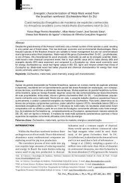
Figure 1.1 – The complexity and extraordinary space between roof (timber carpentry of the XIII c.)
and false ceiling (timber carpentry of the XVIII c.) of the Saint Mark’s church in
Florence, Italy.
Complex timber structures, such as those belonging to the roofs of large monuments, are often
not easy to understand in a expedite way. As the coverings of monuments as cathedrals, public
buildings, mansions or villas show very complicate features, not easy to be understood during the
first inspection. This is not only due to the fact that the system is very elaborate and to the large
number of members but also due to continuous changes and repair past works, mostly with
additional stiffening or propping. The typical result of the history of the construction is the increase
in the number and the heterogeneity of the members, together with a multiplicity of connections and
diversity of supports. This means that the original must be distinguished from the additions and the
2
Chapter 1
replacements. This complexity makes the field of conservation of historical timber structures not
only a challenge but a field much in need of modern research.
1.1
A BRIEF INTRODUCTION TO CHESTNUT WOOD
Chestnut wood will be used in the present study due to its wide use in Portuguese historical
timber structures. Chestnut is the name used for any species of the genus Castanea, deciduous trees
of the family Fagaceae. They are characterized by thin-shelled, sweet, edible nuts borne in a bristly
bur. Chestnuts are classified in the division Magnoliophyta, class Magnoliopsida, order Fagales.
The leaves are simple, ovate or lanceolate, 10-30 cm long and 4-10 cm wide, with sharply pointed
and widely-spaced teeth, incorporating shallow rounded sinuses between. The flowers are catkins,
produced in mid summer. The fruit is a spiny cupule 5-11 cm diameter, containing 2-7 nuts, see
Figure 1.2.
(a)
(b)
Figure 1.2 – Chestnut tree: (a) tree, and (b) detail of the fruits.
Being largely propagated in the past for nut harvesting, chestnut tree (Castanea sativa Mill.),
represents today one of the most diffuse species in the European Mediterranean area. In Portugal,
about 32,000 ha are pure chestnut forests (Fioravanti and Galotta, 1998). During some historical
periods, in various regions of Europe the cultivation of chestnut became so dominant and
indispensable for the survival of mountain populations that some authors do not hesitate to identify
these cultures as “chestnut civilizations” (Gabrielli, 1994). Therefore, several studies and
monographs have been dedicated to the study of chestnut.
The wood of chestnut is considered as moderate shrinking and not easy to dry. It shows high
natural durability and it is therefore well suited for different uses. In the North of Portugal, besides
roof and floor structures, windows and doors have also been manufactured of chestnut wood for
Introduction
3
centuries. The results of investigations (Fioravanti and Galotta, 1998) showed that chestnut sawntimber is also very well suited for glue-laminated timber. Chestnut wood is porous, but it is very
durable in contact with soil and it has been popular for fence and electrical posts, railway ties, and
beams.
In the European standards EN 350-1 (CEN, 1994) and EN 350-2 (CEN, 1994) chestnut wood is
classified as durable and suitable for all applications with and without contact with soil, except of
some particular cases of very extreme conditions. Deppe and Schmidt (1998) assessed the
mechanical properties for different species after nine years of weathering exposure: chestnut wood
showed the smallest decrease of bending strength (about 20%) in comparison with Robinia, Oak,
and Larch.
1.2
THE PORTUGUESE WOODEN TRADITION IN CONSTRUCTION
There are several relevant time periods to point out the importance of wood in Portuguese
traditional construction. The end of the Middle Age was a period of creative energy, where a
changing society tried to keep and to revive tradition based on paradoxes and controversy. In this
context, religious manifestations and profane events occurred with great apparatus and
spectacularity. Wood played also a role in the collective life of medieval societies, in relation with
architecture of the buildings needed for the festive events, and also with military constructions
associated to the effort that the maritime expansion required, during the XV century.
The relevance of carpenters was also stressed during the period of the reconstruction of
downtown Lisbon, after the disastrous 1755 earthquake. The new constructions were based on a
composite wooden structure of plummets, crosspieces and diagonal lines, filled by masonry,
constituting a three-dimensional frame of very high ductility and with an excellent anti-seismic
behaviour. This, so-called “Pombaline” system, represents a genuine Portuguese structural typology
especially conceived to enhance the seismic performance and following the experience in timber
construction. Here “Pombaline” is the term coined after the Marquis of Pombal, the prime minister
at the time of the 1755 earthquake, who took most of the decisions regarding the reconstruction of
Lisbon. Figure 1.3 shows an internal timber wall arrangement example for downtown Lisbon, see
Cóias e Silva et al. (2001) for detailed information.
The traditional usage of wood takes into consideration the local predominance of species but
also its structural or ornamental function. Noble wood, as chestnut, oak and pitch-pine (coming
from the commercial exchange between Portugal and North America in the century XVI), was used
in palaces, in castles or in the interior of churches. This use of noble wood could be combined with
pine or the cypress for wood laths. However, in the North of Portugal the use of oak and chestnut is
predominant in most buildings. In the rest of the country the use of pine predominates.
Wood has been traditionally used in the construction as piles for ground consolidation and for
indirect foundations in case of poor soil conditions, particularly in regions close to water lines and
high ground water level.
4
Chapter 1
Figure 1.3 – Internal timber wall arrangement for downtown Lisbon: example of a composite
timber-masonry wall.
Floors and stairs were frequently made by a system of beams up to 6-7 m of length, with a
spacing around 400 mm up to 600 mm, see Figure 1.4. The dimensions and the transversal sections
vary taking into account the wooden species. For spans larger than 7 m, after the XIXth century and
following the development of the iron industry in the industrial revolution, it was common to use
metallic beams and composite floors as an alternative to the traditional wooden solutions.
(a)
(b)
Figure 1.4 – Typical floor typologies.
The roofs of monumental and historical wooden buildings are probably the most emblematic
structural systems and incorporate the larger structural complexity. The multiplicity of joints and
constructive solutions varies taking into account the evolution of techniques and materials. The
most typical timber roof structures in traditional constructions are the wooden trusses. The trusses
Introduction
5
were mostly made of main roof beams, which received the purlins that supported the rafters, which,
in turn, received the laths that supported the roofing tiles.
1.3
THE ROLE OF RESEARCH ON TIMBER STRUCTURES
In the past, timber structures were erected using traditional methods and rules-of-thumb passed
from one generation to the other. Without mathematical or predictive methods, but with experience
and great skill, an impressive empirical wisdom was obtained.
Presently, prejudices persist against timber structures in several countries, based on the claim
that it is expensive, fragile, burnable, and dependent on unreliable workmanship and unknown
quality. At the present state of knowledge, rational design rules, based on a thorough material
description and a proper validation by comparison with a significant number of experimental results
is available. However, safety assessment of existing structures and characterization of traditional
wooden building techniques remain a true challenge. This means that experimental research in the
behaviour of large-scale timber specimens and in-situ testing are needed. Inspection and evaluation
of the in-situ structural properties represent an important part of the conservation of historical
timber structures, and non-destructive evaluation methods are excellent to achieve a good level of
knowledge in the structural analysis, diagnosis and inspection of ancient constructions
In addition, the introduction of sophisticated numerical tools, capable of predicting the
behaviour of timber structures from the linear stage until complete loss of strength, based on
nonlinear finite element analyses, will always be helpful to better understand the structural
behaviour and to perform parametric studies. In particular, computations beyond the limit load
down to a possibly lower residual load are needed to assess the safety of the structure.
1.4
OBJECTIVES AND SCOPE OF THIS STUDY
The general aims of the present work are: (a) to quantify the strength capacity of wood-wood
mortise and tenon joint by physical testing of full-scale specimens; (b) to evaluate the reliability of
different non-destructive techniques (NDT) for determining mechanical data and joint properties;
(c) to propose adequate correlations between NDT and mechanical data or joint properties for
chestnut wood.
For this purposes, old (OCW) and new (NCW) chestnut wood is used in the experimental
campaign. It is further noted that the strategy adopted has a broad application in other timber joint
typologies.
Other specific objectives of this study are:
− to characterize the elastic and inelastic properties of chestnut wood under compression and
tension parallel and perpendicular to the grain, using destructive and non-destructive
methods. Three non-destructive methods (ultrasonic testing, Resistograph and Pilodyn) are
6
Chapter 1
proposed and the possibility of their application is discussed based on the application of
simple linear regression models;
− to investigate the static behaviour of real scale old timber connections (wood-wood
connections) and to characterize the ultimate strength capacity, the global deformation of
the joint and the failure patterns;
− to validate the adopted nonlinear model by comparing the predicted behaviour with the
experimental behaviour. The adopted model should be able to predict the failure mode and
the ultimate load with reasonable accuracy. Moreover, a parametric analysis should
indicate the most relevant parameters for the structural response.
1.5
OUTLINE OF THE THESIS
Chapter 2 addresses the criteria and methods mostly used to evaluate the residual cross section
of timber elements, and the technological and mechanical characteristics of structural wooden
elements.
Chapter 3 presents a brief introduction to non-destructive evaluation of timber structures and
deals with the most relevant issues concerning the experimental use of the non-destructive
techniques used later in this study to characterize mechanical properties, namely micro-drilling
(Resistograph®), needle penetration (Pilodyn®) and ultrasounds (Pundit®).
Chapter 4 characterizes the compressive properties of chestnut wood under compression
perpendicular to the grain, using destructive and non-destructive methods. The chapter includes also
a proposal to define the ultimate strength value, aiming at an adequate design value. An overview of
testing apparatus and results relevant for practical purposes is also presented. In addition, the
performance of different NDT for assessing strength and stiffness is also evaluated. Extrapolation
of regression models obtained from recently cut wooden material to that obtained from old timber
beams is analysed.
Chapter 5 and Chapter 6 present the compressive and tensile properties of chestnut wood
parallel to the grain, respectively. Again, the performance of different NDT for assessing strength
and stiffness is evaluated, and a comparison between new and old wood is evaluated.
Chapter 7 characterizes the strength capacity of wood-wood mortise and tenon joint,
investigating the static behaviour of real scale old timber connections (wood-wood connections)
and characterizing the ultimate strength capacity, the global deformation of the joint and the failure
patterns.
Chapter 8 presents a finite element nonlinear analysis of the mortise and tenon joint tested in
Chapter 7. The multi-surface plasticity model adopted comprehends a Rankine type yield surface
for tension and a Hill type yield surface for compression. Anisotropic elasticity is combined with
anisotropic plasticity, in such a way that totally different behaviour can be predicted along the
material axes, both in tension and compression. Validation of the model is performed by means of a
comparison between the calculated numerical results and experimental results.
Introduction
7
Chapter 9 presents the summary and final conclusions that can be obtained from the present
study.
8
Chapter 1
Chapter 2
9
Brief review of non-destructive evaluation of timber
This chapter addresses the criteria and non-destructive methods frequently used to evaluate the
residual cross section of timber elements, and the technological and mechanical characteristics of
structural wooden elements.
2.1
INTRODUCTION
Structural evaluation of ancient or recent timber structures present particular problems (related
to inherent wood material properties) and difficulties. In-situ evaluation (without damaging) of
timber structural elements represents an initial and crucial step for the success of the rehabilitation
process. Support for non-destructive inspection works includes nowadays a variety of tools (without
damaging the structures) offering valuable information about the quality and biodeterioration status
of timber elements.
Appraisal and repair of ancient timber structures has become a major topic of interest in the last
decades. In the recent years this renewed interest considerably increased the number of technical
interventions and design developments in Portugal. Conservation or rehabilitation of existing timber
structures imply extensive knowledge about the properties of materials from which the structure is
made. This knowledge constitutes the support for short-term structural behaviour assessment as
well as to foresee the continuous adaptation and capacity of response of the material under longterm actions.
Due to the high variations intra and inter species, a large volume of wooden material is needed
to be tested to characterize its mechanical properties with a minimum level of confidence. Quality
control and preservation of artistic value were considered important issues leading to the
development of some non-destructive test methods for wood which were used in the evaluation of
the mechanical and physical properties of other materials (composite, metals, etc…). The nondestructive evaluation methods are an excellent alternative to achieve a good level of reliability in
the structural analysis, diagnosis and inspection of ancient constructions.
Ross et al. (1998) defined non-destructive materials evaluation as “…the science of identifying
the physical and mechanical properties of a piece of material without altering is end-use
capabilities and using this information to make decisions regarding appropriate applications…”. A
10
Chapter 2
wide variety of tests can be performed with selection dictated by the test performance or property of
interest, depending on the nature and geometry of the object under study.
The efficiency and reliability of NDE (non-destructive evaluation) can be increased if
laboratorial tests are used to study the variability of the mechanical characteristics of the wooden
elements (Uzielli, 1992a; Cruz et al., 1994; Bonamini et al., 2001). For this it will be necessary that
result well coordinate and conduct all the plural-disciplinary activity, which is composed by the
execution, design, safety verification and the retrofitting design of structures. This work should be
coordinated with laboratorial tests providing important information for the evaluation process.
Therefore, laboratorial tests represent a vital role in NDE because they are a mean to explain
properties and characteristics of wood and to validate NDE results.
In particular, the last decades witnessed developments in the testing techniques and equipments
diminishing the subjectivity and increasing the accuracy of structural analysis, diagnosis and
inspection of historical constructions. NDE, which is a term that encompasses a much broader range
of activities than NDT (non-destructive testing) has an own special interest due to the fact that its
use does not affect the present structural integrity and safety of the structure (Bodig, 2000).
In-situ diagnosis of ancient timber structures has been described by several authors (Ceccotti
and Uzielli, 1989; Uzielli, 1992b; Tampone, 1996a; Tampone, 1996b; Ross et al., 1998; Tampone
et al., 2002). All the authors state that an initial visual inspection of the entire structure and of the
singular elements is required in order to determine the original timber characteristics and the
changes suffered due to service conditions. This survey follow several steps, beginning with the
purpose of a general prediction of mechanical properties and ending in a thorough examination
using NDE. But an important characteristic of several ancient timber structures is that they can
effectively bear higher loads than expected (Togni, 1995), which stresses the need of adequate
procedures for diagnostic and assessment of the real bearing capacity, which can not be obtained
with a simple visual inspection. Otherwise, the increasing interest in cultural heritage and
restoration projects can also cause the loss of part of a common European cultural memory.
NDE can be classified in two distinct groups: Global Test Methods (GTM) and Local Test
Methods (LTM) (Bertolini et al., 1998; Ceraldi et al., 2001). The former includes e.g. the
application of the ultrasonic and vibration methods. The latter, being the Resistograph (Rinn, 1994)
and the Pilodyn (Görlacher, 1987) the most common techniques, plays usually a major role in the
support of visual inspection of wooden elements and structures.
Usual applications of LTM are related with the prediction of the element residual section by
analyzing abnormal density variations in the element generally associated with mass loss, which
could be due to biological degradation (Machado and Cruz, 1997).
Other NDE methods can be applied to wood and wood composites namely: thermography
(Bonamini, 1995; Tanaka, 2000; Berglind and Dillenz, 2003), sonic stress waves (Ross et al., 1999;
U. S. Forest Products Laboratory, 1999; Divós, 2000), X-Ray (Lindgren et al., 1992; Bucur et al.,
1997, Bergsten et al., 2001), sniffer dogs (used to identify dry rot fungus in wood), isotope method
(Madsen, 1994; Feinberg, 2005) and endoscopic methods. The development of these and other
Brief review of non-destructive evaluation of timber
11
NDE methods is in fast progress, however, owing to safety concerns, high costs involved, technical
issues, etc., there use has been quite limited in structural timber evaluation.
A semi-destructive method based on testing of small non-standard samples taken from historic
timber structures was developed by Kasal et al. (2003). Two kinds of samples were proposed: i)
thin tension test specimens and ii) the core drilling specimens. Kasal (2005) concluded that a more
reliable estimation of mechanical properties and density was possible since the strength and
elasticity parameters were obtained directly from destructive tests of the material.
Core drilling has been also used in the dendrochronological chronology, analysis of wood
structures and objects and determination of density (Lexa and Tokosova, 1983; Romagnoli et al.,
2004; Bernabei, 2005; Romagnoli et al., 2005). Cores of approximately 12 mm diameter have been
used to determine shear strength of glue lines in the laminate timbers in service (Selbo, 1962).
Other use of the core drilling includes determination of strength characteristics of standard and core
specimens. Theoretically, the mapping between the core strength and standard prismatic specimen
should yield a correlation coefficient close to unity (Kasal, 2003) because sampling corresponds to
conservation requirements concerning limited intervention and it does not influence the load
carrying capacity of a tested element.
2.2
GLOBAL TEST METHODS (GTM)
Visual Inspection and Species Identification – this is the most simple and oldest NDE
method. The visual evaluation consist in examining directly, and preferably at close distance,
checking and registering wood features, signs of damage or deterioration, sometimes with the help
of simple instruments (knife, chisel, hammer, etc.), providing a rapid means of identifying areas that
may need further investigation. This is an essential part of diagnosis but the results depend severely
on the experience of the person carrying out the task. The following aspects should be addressed:
− evaluation of the wood original quality (species and main characteristics of the element,
natural defects such: as spiral grain, knots, ring shakes, discoloration). Small samples of
wood can be removed from the timber members for identifying wood species. This
identification is accomplished by examining the anatomical features of the wood under a
light microscope. Wood species identification restrains the variability of properties
(density and mechanical) and allows the application of models (often regression) obtained
in laboratory for specific wood species. Also it is essential for deciding on the historical
importance of a particular wood element;
− identification and evaluation of biodeterioration through the presence of biological agents
(fungi, insects, etc.) or recognition of damage (bore-holes, wood surface changes, bore dust
near the damaged element);
12
Chapter 2
− global location and relative position, structural function, dimensions, accessibility,
cleanness of the surfaces of the element, light conditions, existence of survey drawings and
their agreement with the actual structural conditions;
− location of the relative position of the attacked zones and problems related with the loading
conditions;
− evaluation of the residual section.
However, the estimation of the serviceability properties of new and/or reconstructed timber
constructions by means of the visual grading method is not entirely reliable due to the many factors
influencing the mechanical properties of timber and, further, the biased influence of the human
factor. Moreover, the information is mostly qualitative.
Ultrasonic Stress Wave – coupled with a thorough visual examination, this technique can add
significantly to the quality of an inspector’s evaluation by providing information on the internal
condition of members and their residual load-carrying capacity (Sandoz, 1989; Machado et al.,
1992; Lemaster et al., 1997; Ross et al., 1997; Ross et al., 1998; Zombori, 2000). Most of these
studies do not show an effective relation between ultrasonic method and the residual load-carrying
capacity of the elements. This can be explained by the wavelength that is generally larger than the
dimensions of the localized defects (knots, slope of grain or other local defect). However, this
method could also be used, with an extraordinary accuracy, to determine some local effect that
could be explored and could allow a good interpretation of the local properties of the elements in
situ.
It is well known that stress waves velocity can be directly related to the elastic properties of
timber since impedance contrasts in the material cause scattering of elastic waves. The propagation
velocity of the longitudinal stress waves in an elastic media depends essentially on the stiffness and
the density of the media itself. On the other hand, it is normally possible to measure the propagation
time of a set of elastic waves in the axial direction of the wooden elements or in the perpendicular
directions to this (it is stressed again that the propagation time is an average time obtained from the
measurement of the faster elastic waves). Presently, different standards emerged to measure the
ultrasonic properties of materials with a particular reference to ASTM E494-89 (1989).
Evaluation of the complex wave-sequence transmission and propagation is a very difficult task
to analyze and interpret: the early portion of the arriving signal is a p-wave; slower components
(mostly composed by shear and surface waves) and reflected waves are not present at this stage,
being the interpretation of the slower components of the wave (Yasutoshi, 2000) one of the most
complex problems. One of the most important advantages of the ultrasonic method is that the wave
is affected solely by the material in-between the two receivers (permitting a relatively
straightforward evaluation).
The last few decades have witnessed extensive research aimed at finding a hypothetical
connection between the propagation of elastic waves in a material and its ultimate strength (Berndt
et al., 1999). Several approaches have been assumed:
Brief review of non-destructive evaluation of timber
13
− the global belief and assumption that material failure results from pre-existing
inhomogeneities in the material (Patton-Mallory and Cramer, 1987; Bodig and Jayne,
1993). These local inhomogeneities change the local elastic properties of the material and
create impedance contrasts which cause scattering of elastic waves, and are usually
interpreted and analyzed by mechanics of composite materials (Kachanov, 1993). The
scattering behaviour is used for mapping unusual reflections in metals, one of the oldest
non-destructive evaluation methods;
− the assumption that the control of the energy dissipation properties and mechanisms are the
same that determine the static behaviour of wood materials (Jayne, 1959; Ross and
Pellerin, 1994), which allows the statistical evaluation of correlations between wave
propagation characteristics (velocity and waveform parameters such as damping,
maximum amplitude, contained energy and spectral parameters of the signal) and wood
strength parameters, such as modulus of elasticity and ultimate strength;
− the acoustic-ultrasonic (combination of conventional ultrasonic test and acoustic emission)
evaluation which was originally developed as a means to assess flaw distribution and the
mechanical properties of wood and wood composites (Vary, 1991; Biernacki and Beall,
1993), but today is used in other applications such as material anisotropy of composites,
high-resolution imaging of wood (Berndt et al., 1999) and detection of decayed wood
(Patton-Mallory and De Groot, 1989).
For prismatic, homogeneous and isotropic elements and for those with a section width smaller
than the stress wavelength, the relation:
E din = V 2 ⋅ ρ
(2.1)
holds, where E din represents the (elasto)dynamic modulus of elasticity (N/mm²); V is the
propagation velocity of the longitudinal stress waves (m/s) and ρ is the density of the specimens
(kg/m³).
For practical purposes, the relation between the dynamic modulus of elasticity and the static
value is particularly relevant ( E din ≥ 0.90 ⋅ E sta ). This relation is explained by the viscous-elastic
behaviour of wood (Bonamini et al., 2001). Generally a linear relation is adequate (U.S. Forest
Products Laboratory, 1999; Bonamini et al., 2001):
E sta = a × E din + b
where a, b are constants depending on the material.
(2.2)
14
Chapter 2
The propagation of elastic waves is affected by local elastic properties of the material.
Depending on the wavelength and element dimensions, the measured properties are averaged over
differently sized regions. Thus, the propagation velocity of elastic waves in a particular mode,
together with the material density, show immediately information on the stiffness coefficients of the
material. Finite element modelling showed how a wave propagates in an orthotropic material in
various directions with respect to the fiber orientation (Lord et al., 1988).
These and other fundamental efforts, coupled with advances being made in the evaluation of
connections (Pollock et al., 1996) and structural systems, suggest this method as one of the most
used in timber evaluation (see Figure 2.1).
Figure 2.1 – Ultrasonic stress wave method (parallel to grain emission).
The ultrasonic method, which is very similar to the sonic stress wave method but uses higher
frequencies (20 kHz-100 MHz), is often used in homogeneous, non-porous materials. In wood and
wood composites materials it is less effective due to the porous and inhomogeneous nature of the
material (Beall, 1987). Low frequencies (20 kHz-500 kHz) are often used in wood because of high
wave attenuation (Zombori, 2000).
The velocity of ultrasonic stress wave travelling through a solid is dependent on its elastic
properties. In high dispersive materials as wood, while travelling inside the material the wave
suffers a series of reflection events originating new waves with different polarizations and each
having a characteristic velocity. Most of ultrasonic equipments available considers only the fastest
wave (showing a minimum of energy – generally defined by a volt threshold limit) to arrive at the
receiver probe. It is expected that this wave travels through the highest quality zones of a wood
element bypassing weaker zones (showing, knots, decay, slope grain) and therefore not allowing the
local characterisation of that wood element, see Figure 2.2.
Brief review of non-destructive evaluation of timber
15
Figure 2.2 – Ultrasonic stress wave propagation and influence of defects.
If the signal is deviated, the transit time increases. Despite of their inhomogeneity, anisotropy
and natural patterns of variability (inter and intra specie), it is possible to correlate the efficiency of
wave propagation with the physical and mechanical properties of wood: high propagation velocities
are associated with greater fracture resistance and absence of material defects.
Excellent results have been obtained using the velocity of propagation (both in longitudinal or
transversal direction) for the estimation of the (elasto)dynamic modulus of elasticity and to quantify
and locate decayed wood (Togni, 1995; Ross et al., 1997; Machado, 2000).
Coupling of the transducers to the specimen surface is a major problem of the ultrasonic
method. The presence of air is an inhibitor of the transmission velocity (different acoustic
impedance), so it is necessary that the transducers are adequately coupled to the specimen surfaces
during testing. Good coupling between the transducers and surfaces is guaranteed by a proper
grease and pressure.
Another relevant issues regarding ultrasonic inspection of timber elements comprises the
dimensions of the elements which often limits the choice of wave frequency (due to the high
attenuation of the wave) and therefore the size of the defects able to be detected and the
impossibility of getting free access to opposite faces of the elements which limits the method
(transmission or shadow). Since high frequency stress waves attenuate significantly over relatively
short distances in wood (particularly for wave propagation across the grain), the ultrasonic method
is primarily effective in relatively small regions of wood members (Szymani and McDonald, 1981;
Ross et al., 1996; Emerson et al., 1998; Ross et al., 1998; Bonamini et al., 2001; Tampone et al.,
2002). The requirements for access to opposite faces of timber members has been partially
overcome with the development of techniques for introducing critically refracted longitudinal wave
energy into wood (Dickens et al., 1996).
Other open questions are the influence of environmental factors and wood characteristics in the
ultrasonic method. For instance, ultrasound velocity increases as the moisture content of wood
decreases. Due to the high hygroscopicity of wood the moisture content represents an important role
when one is analysing the mechanical and physical properties of the material. For Red-Fir, Sandoz
16
Chapter 2
(1989) proposed a reduction of 0.8% in the velocity of propagation for each 1% increase of
moisture content, in a range between 5-30% of moisture content. This author reported also that the
velocity of propagation is sensitive to grain direction. For Maritime Pine (Pinus Pinaster Ait.),
Machado (2000) concluded that increasing the moisture content decreases the longitudinal and
transversal velocity of propagation.
The ultrasonic wave velocity is around three times faster in longitudinal direction than in
transversal direction, which enables sometimes this method to efficiently detect defects that evolves
changes in grain direction, such as knots and spiral grain (Zombori, 2000). Discontinuities in the
cells anatomy or the presence of surface decay caused by insects reduce the ultrasonic wave
velocity. The velocity of propagation in decayed wood is slower because of its anatomic properties,
which can include sometimes holes provoked by biological agents.
Finally, another factor that can be of relevance is the loading condition of the elements. Bucur
(1995) observed, in the three directions of propagation of small specimens of Red-Fir, a small
increase of the velocity of propagation for low stresses (up to one-fifth of the ultimate strength). For
higher stresses this author observed a fast decrease with load increase.
In most of the recent studies involving this method the aim was to control the wood quality as a
final product or as raw material (Machado, 2000) and to inspect historic structures (Sandoz, 1989;
Ross et al., 1996; Ross et al., 1999; Ross and Hunt, 2000). Some of the studies try to focus on the
distinction between clear wood and decayed wood, comparing the results and creating “evaluation
maps”, with experimental results in clear wood that could be adopted in future interventions (Shaji
et al., 2000). Other authors tried to determine residual strength of structural elements that were used
in ancient constructions or that were attacked by biological agents (De Groot et al., 1998), or tried
to determine qualitative properties by modelling wood as a homogeneous isotropic material,
assuming that the clear and the defected wood can be modelled as a fluid, neglecting bending
stiffness (Fransson and Nilsson, 2001).
Among the NDE methods special attention seems to be paid to the ultrasonic technique due to
its fast execution, efficiency, precision, relative simplicity of use and transportation. However, the
technique requires an experience operator and coupling between probe and specimens.
Density Method – density is a current classification criterion of wood due to the relation
between density and mechanical strength values. Correlations between mechanical properties and
density were reported by several authors (Kollmann and Coté, 1968; Bodig and Jayne, 1993;
Giordano, 1999; U. S. Forest Products Laboratory, 1999) for different species, even if often only
weak correlations could be found.
The density determination can be done laboratorially in small dimension specimens extracted
from the elements or can be determined using non-destructive methods (local test methods) in situ
that could be constrained by various factors: firstly, measurements are costly in terms of manpower
and money because they involve extraction and processing of cores. Another important factor is
that, in many situations, density determination has to be restricted to few samples due to the
Brief review of non-destructive evaluation of timber
17
destructive testing performed to obtain the test pieces. This restriction affects the representative of
the sample.
2.3
LOCAL TEST METHODS (LTM)
Drill Resistance (Resistograph Method) – the drill resistance measure by the Resistograph
device is based on the resistance offered by the material to the advance of a small diameter drill bit.
Rinn et al. (1996) found that the mean resistance levels of the Resistographic profiles closely
correlate with the gross density of dry wood from X-ray density profile (with the Resistograph
resolution being smaller than the X-ray resolution). Helms and Niemz (1994) previously related the
resistance profile with member density and radiographic analysis.
In the past, core sampling using conventional drills (φ = 10 to 40 mm) was used to determine
density properties of wood products. But these methods are hardly suited for determining density
variations of structural timber due to the large boreholes.
The Resistographic method is considered a quasi-non-destructive method because the size of the
hole in the specimen after testing does not have any weakening effect. This test allows to obtain the
density profile of specimens/elements, which is the graphical representation of the values of the
drill resistance versus the penetration depth (up to 50 measuring points per mm). The profiles reveal
variations in the density of earlywood and latewood layers thus indicating decayed wood. From
drops in the profiles it is possible to define different stages of deterioration. Also it allows the
detection of discontinuities (for instance fissures).
The equipment used in the present work, see Figure 2.3, measures the resistance of a small
drilling needle (φ = 3 mm) through the power consumption of the drilling device.
Figure 2.3 – Resistograph equipment.
Since the electronic resolution of current equipments is 12 bit (effective signal resolution of 10
bits), the ordinate values of the Resistographic chart vary from 0 to 4095 (Rinn et al., 1996). The
18
Chapter 2
stroke of the needle is constant and the needle rotates continuously (Rinn, 1993; Rinn, 1994a; Rinn,
1994b; Rinn et al., 1996). The needle design eliminates the excessive drill energy consumption
through friction in deeper penetrations: shaft diameter is 1 to 1.5 mm and maximum length is
1500 mm (maximum drilling depth is 950 mm). The tip of the needle has a special geometry and
grinding. The drill resistance concentrates at the tip because its width is double the width of the
shaft (2 to 3 mm). The device contains two engines: one for constant feed and one for the rotation
of the needle. The needle shaft is stabilized continuously inside the drilling device by a special
telescope.
This evaluation method provides information about conservation of the structural elements and
(indirectly) about their structural capacity, such as beam cross section (when it is not possible to
directly measure the dimensions), the residual cross section (decayed wood ≈ lower penetration
resistance of wood), the distribution pattern of annual growth rings (Wang et al., 2003; Frattari and
Pignatelli, 2005), the presence of natural defects and decayed wood not externally visible
(important in architectural details such as beam butts). Some advantages of the method are the
graphical resolution, the simplicity of storing data, of transporting the equipment and performing
the tests (Machado and Cruz; 1997).
Some studies reveal limitations of this method, namely related to the difficulties in carrying out
some inspections/tests due to the location of the element (difficulty in positioning the device
perpendicularly to the element), the testing procedure itself (requires usage of both hands and the
drill must be perpendicular to the surface), the measurements of only local characteristics of the
elements and the invasive nature of the drill resistance technique (Bonamini, 1995a; Emerson et al.,
1998). Therefore, the resistographic method may be best employed if used in conjunction with NDE
methods and techniques that provide qualitative condition assessment or more global condition
assessment.
Some researchers (Görlacher and Hättich, 1990; Isik and Li, 2004) reported relatively moderate
correlation between drilling resistance and wood density (r² ≈ 0.21-0.69), showing that this
correlation has not yet been adequately developed for use in in situ quantitative evaluation. It is
noted that moisture content of wood has a large influence on the density values and Machado and
Cruz (1997) observed that the drilling resistance decreases as moisture content increases. Works
show that the resistance drilling data correlate well with the X-ray densitometry measurements
(Rinn et al., 1996).
Nowadays, the resistographic method is one of the most used methods and several campaigns
were carried out using this technique (Tampone et al., 2002; Augelli et al., 2005a; Meade and
Anthony, 2005; Branco et al., 2005).
Pilodyn Method – similarly to the Resistograph the Pilodyn wood tester is an alternative for
fast and non-destructive estimate of wood density (Hoffmeyer, 1978). The Pilodyn method using
the Pilodyn 4JR, or similar equipment, can be understood as an adaptation and evolution of the
soil’s dynamic penetration test (Giuriani and Gubana, 1993; Ronca and Gubana, 1998) or the
concrete sclerometer (Malhotra, 1984). The Pilodyn wood tester was originally developed in
Brief review of non-destructive evaluation of timber
19
Switzerland to obtain quantitative data on the extent of soft rot in wooden telephone poles, and was
used with the aim of correlating the density of each specimen/element with the depth reached with
the pin of the device. Density is a parameter well related to wood hardness, as it is fairly related
with all the wood properties (Panshin and De Zeeuw, 1980; Bonamini et al., 1995b). The method is
widely used today for evaluating pole decays, or standing trees or sawn lumber density. It is noted
that only the surface hardness or resistance to superficial penetration is measured, which represents
a disadvantage.
There are several versions of this device, more powerful or simply with a different testing
philosophy, that can be used in the evaluation or diagnostic inspections of wood species showing a
high resistance to superficial penetration or in particular situations. These devices like the Pilodyn
12J and the Pilodyn 18J, which possess a spring with a higher stiffness (increasing strike force), or
like the Pilodyn 4JR, which allows a repeating shot, are used to measure parameters related to
density of the specimens. These are dynamic devices based on the action of a calibrated spring able
to drive a flat-head steel pin into the surface of the specimen.
The Pilodyn model 6J for single shot (see Figure 2.4) and model 4JR for repeated shots are
devices that allow to measure the penetration of a metallic pin with 2.5 mm of diameter into wood,
through the release of a spring-loaded pin that transforms the elastic potential energy into impact
energy. This dynamic impact is responsible for the penetration of the pin in the surface of the
specimens, allowing to register the depth penetrated. The density of the wood or the degree of decay
in the wood can be assessed by the different spring energy absorbed by the specimen (Zombori,
2000).
Figure 2.4 – Pilodyn 6J.
A possible broad application of Pilodyn is to sort logs into broad density classes, making the
prices based not only on log size and visual grading but also on density characteristics (Graves et
al., 1996; Watt et al., 1996). In standing trees pin penetration is likely to vary according to normal
density variations patterns present in annual ring of Softwoods and ring-porous Hardwoods (Sprage
et al., 1983). Other applications are the genetic control of species (Aguiar et al., 2003), however
20
Chapter 2
there is the need to monitor some field trials for a longer period of time to confirm and support the
results.
Watt et al. (1996) found that the Pilodyn is able to predict mean outerwood density values with
reasonable accuracy, and offer an alternative to the slower and more costly core sampling. These
authors calibrated the Pilodyn results in specimens of different size against X-ray densitometer
values. Görlacher (1987) obtained good correlation coefficients between density and depth of
penetration of the Pilodyn 6J, taking into account that the number of measurements for each
specimen must be large. This author proposed empirical relations between the depth of penetration
and density, showing that these empirical relations are affected by moisture content. The correlation
coefficient varied from 0.74 to 0.92, and depended on number of measurements and species,
therefore, species-based calibrations are required.
Studies were also carried out to define correlations with mechanical properties. Relations
between resistance to superficial penetration and a three point loading test were found but more
studies are needed to corroborate these results, due to its empirical nature and to the local and
superficial character of the results obtained (Togni, 1995).
For the determination of the modulus of elasticity, Turrini and Piazza (1983) proposed an
empirical relation correlating impact force and modulus of elasticity. The authors proposed also the
adoption of a reduction factor of the modulus of elasticity based on a visual grading of the elements:
80% for non-defect elements and 50% for elements presenting knots, spiral grain, shakes or small
decay portions. Again, it is noted that the penetration depth is highly affected by the moisture
content (Bonamini et al., 2001).
2.4
CASE STUDIES: IN-SITU ASSESSEMENT OF WOOD STRUCTURES
Non-destructive evaluation has been used to examine structures for over 100 years. Methods
used alone, or at the same time with other NDE techniques allow to understand wood structural
behaviour. Ross and Pellerin (1994) prepared a report reviewing pertinent laboratory investigations
designed to explore fundamental concepts and presented several examples of how to apply these
concepts to in-situ assessment of wood members. Machado (2000) also presented some work in this
field.
Table A.1, presented in Annex 1, summarizes some research conducted on the use of several
non-destructive techniques for in situ evaluation of wood members.
Chapter 3
21
Adopted testing equipment and procedures
The present section presents relevant issues about the experimental utilization of the non-destructive
techniques used in this thesis to assess mechanical properties.
3.1
DENSITY DETERMINATION
Wood density is of key importance in the evaluation and characterization of the mechanical and
physical behaviour of wood. Density is correlated with strength properties and its value is
determined by the ratio cell wall to cell cavity, which in turn is function of the relative proportion of
different cell types present in Softwoods and Hardwoods species.
Density was measured according to EN 408 standard (CEN, 2000). Given the conditioning of
the specimens, the average density ρ m is determined for a moisture content of 12%, given by:
ρ12% =
m12%
V12%
(3.1)
Here, m indicates the mass and V indicates the volume.
3.2
ULTRASONIC PULSE VELOCITY METHOD
The methodology followed was based on the transmission method (or shadow method), which is
based on two transducers located in two opposite faces, one as transmitter and the other as receiver.
As mentioned in Machado (2000) this is the best method for wood due to the high roughness
generally associated with wood surfaces and the high attenuation coefficients.
During the tests, the ultrasonic equipment Pundit Plus (Portable Ultrasonic Non-destructive
Digital Indicating Tester Plus) was used (CNS Electronics, 1995), with cylinder-shaped transducers
of 150 kHz composed by piezoelectric ceramic crystals involved in a steel box. Machado (2000)
found that the frequency is lower than the value indicated by the manufacturer because the final
frequency response of the probe function is not only a function of the crystal resonance frequency
(150 kHz) but from the assemble of steel box and crystal (as mentioned by the manufacturer).
22
Chapter 3
In all tests, coupling between the transducers and specimens was ensured by a conventional hair
gel. A constant pressure was applied by means of a thick (2 mm) soft rubber spring, allowing
adequate transmission of the elastic wave between the transducers and the specimen under testing,
and transmitting the coupling force without loading the transducer.
Conventionally wet couplants have been used (glycerine, silicone grease and water) since they
assure an efficient wave transmission energy between the probe and the specimen under inspection.
However, wet couplants penetration on the specimens could damage or contaminate the specimens.
Dry couplants (usually elastomeric materials) and air couplant have been tested more recently with
some degree of success (Machado, 2000). Still the need for a constant and controlled contact
pressure (dry couplants) and field operation restrictions have limited the use of these coupling
solutions. Therefore in the present research a gel is used as couplant since it assures a reliable time
of flight readings (less sensible to contact conditions) and it can be easily used in practice (easy to
be removed without staining the wood).
The rubber spring used allows adequate coupling pressure eliminating micro-gaps ad promoting
a satisfactory coupling interface (wood/transducer) making a more uniform stress distribution
within the coupling interface. Theoretically and practically the increase in the surface pressure does
not significantly improve coupling after a certain level (Biernacki and Beall, 1993; Divós et al.,
2000). Machado (2000) referred that the velocity of propagation of the ultrasonic wave is not
significantly affected by the level of pressure applied (since it is merely dependent on an amplitude
value – trigger – that determines the propagation time), affecting mostly wave shape-related
parameters (total energy, amplitude, etc…).
Transducers lack of alignment can be a possible disturbance factor on repeatability of readings.
Most specimens show a surface waviness or roughness that can easily affect that alignment. To
avoid misalignments two wooden guides were used to set the transducers in the wood specimens
surface and align them, see Figure 3.1.
The tests were conducted on samples sufficiently large, perpendicularly to the propagation
direction, to avoid sample edge effects on wave propagation. Since generally the behaviour of
elastic waves scales with the wavelength, sizes relate to the respective wavelengths in the direction
of interest. Ideally, the dimensions perpendicular to the propagation direction would be an order of
magnitude larger than in the propagation direction.
Adopted testing equipment and procedures
(a)
23
(b)
Figure 3.1 – Test set-up and alignment of the transducers: (a) front view, and (b) top view.
One correction is imperative when the dimensions of the section of the specimens are smaller
than the wave length (λ). In the present work the wave frequency (f) was 150 kHz, the maximum
velocity of propagation (V) was 5859.4 m/s (Direct Method, parallel to grain) and using the
following relation:
⎛1⎞
⎟⎟
⎝f ⎠
λ = V ⋅ ⎜⎜
(3.2)
one can obtain the wave length of 39 mm, which is smaller than all the specimens dimensions
(50 mm). This can spatially be interpreted as a spherical surface, in comparison with the specimens’
dimensions, which represents the shape of the front wave. In this situation one must use the follow
relation:
E din = V 2 ⋅ ρ ⋅
(1 + ν ) ⋅ (1 − 2ν )
(1 − ν )
(3.3)
where Edin represents the (elasto)dynamic modulus of elasticity (N/mm²); V is the propagation
velocity of the longitudinal stress waves (m/s), ρ is the density of the specimens (kg/m³) and ν is
the coefficient of Poisson. However, the simplified relation:
E din = V 2 ⋅ ρ
(3.4)
24
Chapter 3
was used due to the difficulties of characterizing each one of the six coefficients of Poisson. Since
results obtained by this research program (reported in Chapters 4, 5 and 6) and other authors show
that no significant variation of these coefficients exists within the same wood species, the equation
parcel related with these coefficients can be envisage as a constant dependent only on the type of
wood species.
3.2.1 Compression perpendicular to the grain
Although three methods were used in the framework of a more general approach, see Figure 3.2,
(Indirect Method; Direct Method parallel to the grain, and Direct Method perpendicular to the
grain), the Indirect Method was the only method correlated with the principal mechanical
characteristics of the specimens, since it is the most appropriate in practical cases. The Indirect
Method can be used for evaluating different zones of the element (global or local evaluation) and
only needs a face of the element to be accessible.
Figure 3.2 – Ultrasonic pulse velocity: all the used methods.
The transmission technique of elastic waves based on the Indirect Method was used in all the
faces, for the case of diagonal and diffuse tests specimens, see Figure 3.3a. For the case of radial
and tangential tests specimens, the transducers were used in two opposite faces, depending on the
orientation of annual growth rings. In all cases average values were considered in all measurements
and two readings per specimen were generally made but a third one was added if the two first
readings differed significantly, see Figure 3.3b.
Adopted testing equipment and procedures
(a)
25
(b)
Figure 3.3 – Compression perpendicular to the grain: (a) annual growth rings orientation along the
direction of the load, and (b) Indirect Method test set-up.
Regarding the Direct Method parallel to the grain, it requires access to the ends of the elements
(in most cases not possible) and allows only a global evaluation of the material (it is not possible to
evaluate weak or critical zones in the element), see Figure 3.4a.
Finally, the Direct Method, perpendicular to the grain, only gives a local evaluation of the
element and it needs access to two opposite faces. In this method contiguous sections of the same
specimen were used (the distance between each section was 6 cm), see Figure 3.4b. The results of
these two last methods are presented in Annex 2.
(a)
(b)
Figure 3.4 – Test set-up: (a) Direct Method, parallel to the grain, and (b) Direct Method,
perpendicular to the grain.
26
Chapter 3
3.2.2 Compression parallel to the grain
In the specimens tested in compression parallel to the grain, the ultrasonic tests were carried
with two types of signal transmission: i) Direct Method, parallel to the grain, and ii) Indirect
Method, see Figure 3.5. In this case, only the transmission technique of elastic waves based on the
Direct Method, parallel to the grain was used. The elastic properties of wood were estimated by the
measurement of stress wave propagation time and average values of the propagation velocity of the
longitudinal stress wave were considered in all measurements. At least two readings per specimen
were generally made but a third one was added if the two first readings differed significantly. The
results of the Direct Method, parallel to the grain, are presented in Annex 3.
(a)
(b)
(c)
Figure 3.5 – Test set-up: (a) Direct Method, parallel to the grain, (b) Indirect Method, and (c) the
two distinct methods used.
Adopted testing equipment and procedures
27
3.2.3 Tension parallel to the grain
Finally, in the specimens tested in tension parallel to the grain three different kinds of emission
tests were realized: i) Indirect Method (d = 20 cm); ii) Indirect Method (d = 45 cm) and iii) Direct
Method, parallel to grain, see Figure 3.6.
Figure 3.6 – Ultrasonic tests: the three distinct methods used.
The transmission technique of elastic waves based on the Indirect Method (d = 20 cm and
d = 45 cm) was used in both faces, see Figure 3.7a and Figure 3.7b. In all methods average values
were considered. In the Direct Method, parallel to grain, the measurements were made as
represented in the Figure 3.8, and once more average values were considered.
(a)
(b)
Figure 3.7 – Ultrasonic tests: (a) Indirect Method (d = 20 cm), and (b) Indirect Method (d = 45 cm)
and comparison between the two specimens (the standard and the adopted).
28
Chapter 3
Figure 3.8 – Ultrasonic tests: Direct Method, parallel to grain.
3.3
RESISTOGRAPH METHOD
The use of the Resistograph allowed to obtain the density profile of the used tests specimens,
see Figure 3.9. The Resistograph is usually adopted to obtain density profiles and, in the present
testing program, drilling was made on planes TL or LR, which, in real cases, represents the
accessible faces of timber elements. For each specimen, three independent profiles have been
carried out and the results shown represent the average of the readings. Here, R, T and L are
respectively the radial, transversal and longitudinal directions, where the grain corresponds to the
longitudinal direction.
(a)
(b)
Figure 3.9 – Resistograph device: (a) global view of the equipment, and (b) drilling a specimen.
For all the specimens, as a function of the obtained graphs with the Resistograph, a
resistographic measure (RM) was calculated. The ordinate of the Resistograph profiles reveals a
Adopted testing equipment and procedures
29
relative measure for the power consumption of the drilling equipment, which cannot be controlled
by the user. This is acceptable in most applications because scaled values are sufficient, for
detection of tree rings and decayed wood. For structural or mechanical usage, quantitative and
absolute values are required.
The adopted resistographic measure represents the ratio between the integral of the area of the
diagram and the height of the tests specimens (see Eq. 3.5), which is an average value. Using this
quantity, the Resistograph results can be compared with the values of density and the strength
values, even if the value remains scaled.
The RM value is given by:
h
RM =
∫ Area
(3.5)
0
h
where h is the height (drilling distance) of the specimens.
A workbench and a tripod were used to execute the drills reducing the possibility of error, by
accurately controlling the specimen position and execution time.
3.4
PILODYN 6J METHOD
The dynamic impact provided by Pilodyn 6J is responsible for the penetration of the pin in the
surface of the specimens, see Figure 3.10. The penetration depth is recorded while the Pilodyn 6J is
still pressed against the tree. The penetration is read in millimetres (0-40 mm, without decimals) on
the scale on one side of the instrument.
(a)
(b)
Figure 3.10 – Pilodyn 6J device: (a) global view of the equipment and parts, and (b) specimen under
testing (the depth reached can be read from the scale).
30
Chapter 3
The Pilodyn 6J was used with the aim of correlating the density of each specimen with the depth
reached with the pin of the device (surface hardness or resistance to superficial penetration).
As in the case of Resistograph the tests were made on planes TL or LR, which, in most real
cases, represents the accessible face of timber elements. The shot was made at an angle of 90º
between the direction of penetration and the tangent to annual growth rings. This way undesirable
variability of the results due to the orientation of annual growth rings is eliminated. Occasionally, it
was necessary to select shot locations so that local defects would be avoided.
For each specimen, the average value of the four faces was considered. Three readings per
specimen were made but a fourth one was added if the four first readings differed by more then
2 mm. Apart from regularly cleaning and occasional calibration, the pin was replaced every 500
shots. In the entire testing campaign, bending or crushing of the pin was never observed.
Chapter 4
31
Chestnut wood in compression perpendicular to the
grain. Evaluation by non-destructive methods
In traditional timber framed buildings the structural system is usually designed in such a way that
load is transferred perpendicular to the grain using joints between walls and floors that are easy to
produce and assemble (Blass and Görlacher, 2004), see Figure 4.1.
Figure 4.1 – Timber frame building.
The primary effect of compression perpendicular to the grain is compaction of the wood fibers.
With higher fibers compaction, load carrying capacity increases due to density increase.
Compressive stresses may be self-imposed, as in seasoning (shrinkage forces perpendicular to the
axis of the tree), in drying and in pulping, or mechanically imposed, as in production of wood
composites products. But such compressive stresses can generally be found in timber structures
such as trusses, where tie beams, also referred to as crossbeams, anchor-beams, ties and lower
chords, are transverse horizontal members that span from wall to wall, resisting the outward thrust
of roof planes. Where a tie beam meets the wall framing, a tying joint is formed. Some of these
joints are “mysterious” since their configuration and method of assembly are a mystery until they
are disassembled. Because truss spans are often large, very substantial forces can develop in
elements and mainly in joints.
32
Chapter 4
Compression perpendicular to the grain is often critical in different situations of timber design.
It is usually most severe at the ends of deep, narrow beams, and in the connecting members at the
ends of short, heavily-loaded columns. In most cases, these compressive stresses are usually low but
this does not apply to large and heavy timber beams and timber truss rafters (Korin, 1990). These
stresses can occur concentrated over a portion or distributed over the surface of a specimen.
Examples of concentrated loads are a post resting on a sill, sills continuously loaded in compression
perpendicular to grain sliding sideways or a rail on a crosstie (which is the basis for standard tests).
A final example is the intermediate support of a continuous beam, where compression perpendicular
to the grain can lead to bending failure.
But there are situations where elements are transversely loaded along all its length, e.g. in
mining timber, foundation elements or frame wooden (see Figure 4.2). It is then necessary to fully
understand the strength capacity of these timber elements or systems in order to design adequate
strengthening solutions and to eliminate possible original design misconceptions.
(a)
(b)
Figure 4.2 – Timber structural systems transversely loaded along their length: (a) wooden mining
vault, and (b) wooden frame.
From an engineering point of view one of the most important questions is that structures are
usually designed to respect simple execution, economy, adequate structural behaviour and safety of
the occupants. In theory it is possible to design joints so that load transfer perpendicular to the grain
is avoided, but this is not feasible considering all other aspects of the design.
When a uniaxial compressive stress is applied to a specimen, the following types of deformation
may take place: elastic or plastic shortening in ductile materials, crushing and fracture in more
brittle materials, sudden out-of-axis instability (buckling) in long, slender bars, or combination of
all these. A material such as wood commonly fails along a diagonal plane that is not the plane of
maximum compressive stress, but rather one of high shear stress, which accompanies uniaxial
compression. Deformation perpendicular to grain is crucial in joints, especially for multi-storey
timber frame buildings, where displacements at each level can add up to substantial movements
over the building height.
Chestnut wood in compression perpendicular to the grain. Evaluation by non-destructive methods
33
It is easy to understand that these large displacements have adverse consequences in structural
systems as excessive deformation damages non-structural elements such as windows, doors and
renderings. In general, this situation can be controlled by imposing limits to ultimate stress but
Thelandersson and Mårtensson (1997) defend a more sophisticated philosophy for the design of
wood loaded perpendicular to grain.
4.1
BACKGROUND
4.1.1 Influence of wood characteristics
From the studies aiming to characterize the physical-mechanical properties of wood when
loaded in compression perpendicular to the grain, some factors seem particularly relevant for the
interpretation of results.
Density is one of the main factors that influence the wood behaviour. When loading parallel to
grain occurs, strength tends to be linearly dependent on density. However, if loading is
perpendicular to grain, it is frequent to adopt a nonlinear relation given by:
f c ,90 ≈ ( ρ )α
(4.1)
Here, f c ,90 is the transversal compressive strength, ρ is the density and α is a constant ranging
between 1.5 and 2.3. This value depends on growth rings orientation, specimen dimensions and
criteria for definition of failure. In the absence of more information, a value of α equal to 1.7 is
recommended (Gehri, 1998).
A criterion for definition of failure assumes a major role due to the different approaches of
structural behaviour on wood constructions. Figure 4.3 shows typical stress-strain diagrams for
radial and tangential compression. The letters in the graph represent notable diagram points that
correspond to: A and A’ – specimens after the accommodation load; B and B’ – first failure at a
strain around 3%; C and C’ – for a strain around 10% and D and D’) for a strain around 20%.
As frequently happens, the behaviour of elements with structural dimensions, when loaded in
direction perpendicular to grain, is extrapolated from the behaviour of wood specimens without
defects. Understanding the influence of annual ring patterns on the mechanical properties of wood,
and knowing that the behaviour is characterized by a total absence of a clear failure of the material,
three deformation levels may occur and be easily identified when, for example, a radial specimen is
loaded: i) initial elastic deformation; ii) plastic level (buckling of cellular walls and failure) and
iii) densification (Bodig, 1965; Tabarsa and Chui, 2000; Tabarsa and Chui, 2001). This failure
mode is associated with relatively high displacements on wood.
34
Chapter 4
Figure 4.3 – Typical stress-strain diagrams (up to 20 percent compressive strain) of a ring porous
wood in transverse compression (Bodig, 1965).
Characterization of physical-mechanical behaviour in compression perpendicular to grain, as a
function of the orientation of the annual growth rings, becomes a fundamental step from a structural
point of view. Taking into account the load direction towards the annual growth ring orientation,
Youngs (1957) showed that normal to the grain tension behaviour of pieces with 0 to 45º
inclinations (relatively to the annual growth rings) was similar, only differing for 90º angles. In
compression, the behaviour it is not exactly the same, namely on the differences between failure
mechanisms for orientations mentioned above. For 45º inclinations, strength is lower than in radial
and tangential loads situations.
The stress-strain diagram shape can be justified by wood’s anatomy. Load alignment with the
three principal wood axis is mainly responsible for the different patterns found in stress-strain
diagrams obtained from compression perpendicular to grain tests. This variable can be more
important than differences between wood species (Bodig, 1965; Bodig, 1969).
Kollman (1959) showed that the annual growth rings properties are crucial on the transversal
compression control. Porosity ratio in the hardwood rings or contrast of density between
summerwood/springwood on coniferous are determinant factors on the characterization of
transversal compression. Intermediate orientation of the growth rings and wood rays, between the
tangential and radial position were also been identified as influence factors on the mechanical
characterization process. This author concluded that strength in transversal compression was
reduced to a minimum value for approximately 45º of the annual growth rings and wood rays
inclination, in relation to the load direction, which is corroborated by the general composite
materials elastic theory. Ethington et al. (1996) shown that compressive strength perpendicular to
the grain depends and is related, in an approximately quadratic form, with the orientation of the
annual growth rings.
Hall (1980) concluded a study in which the influence of the orientation of the annual growth
rings on several species was evaluated. The author obtained the strength values of the different
resinous species, as well as the correspondent modulus of elasticity, adopting a criterion based on
Chestnut wood in compression perpendicular to the grain. Evaluation by non-destructive methods
35
an extension of 0.2%. Madsen (1989) corroborated these results and presented more detailed
correlations.
However, in practical situations, the influence of the annual growth rings along the direction of
the load is not so clear; this is due to the absence of wooden elements with sections showing a
particular orientation. Therefore, tests should be made using randomized growth orientations, taking
into account that the failure mode observed for 45º inclinations (which provides lowest strength
values for transversal compression), which is common in prismatic standardized specimens without
apparent defects, is rarely observed when structural dimensions specimens are used and in real-life
situations.
Schniewind (1959 in Bodig, 1965) determined the elastic properties of selected microscopic
wood components – such as the wood ray – and concluded that the cause of lower modulus of
elasticity in the tangential direction could not be explained only by the annual growth rings
arrangement but rather by the presence of wood rays. Kunesh (1968) also justified the differences in
tangential and radial inelastic behaviour of yellow poplar by the presence of wood rays, based on
their influence in the increase of elastic and inelastic properties.
Depending on shape and dimensions, thickness and stressed area, different relations between
strength and elastic properties of wood may be obtained. Bodig (1963) found that nearly all
mechanical properties of Douglas-fir in radial compression were affected significantly by the
thickness of specimens. Kunesh (1968) observed that, in radial compression for western hemlock
and Douglas-fir wood, the maximum stress decreased with increasing thickness and moisture
content. This author concluded that there will always be a weak portion of rays located in an
earlywood layer in any specimen and with increasing thickness the probability of occurrence of an
extremely weak ray, or several of them, is increased. Other elastic properties such as modulus of
elasticity were also influenced by the specimen geometry, (Bodig, 1963; Bodig, 1965; Kunesh,
1968) increasing with thickness and decreasing with moisture content and stressed area.
Some authors pointed out that wood behaviour in radial compression is strongly dependent on
its anatomical features (Alexiou, 1994; Tabarsa and Chui 2001; Müller et al., 2003). But others
authors believe that elastic behaviour is more dependent on density than on anatomical
characteristics (Kennedy, 1968; Beery et al., 1983). Defects as number of knots, its location and
kind, grain inclination, variations on width and spacing between growth rings and presence of
reaction wood, influence to great extent wood behaviour in compression perpendicular to grain.
However, values given in technical standards and literature for strength and stiffness properties do
not usually consider reduced sections taking into account the presence of defects. Also important
factors are the long-term behaviour and moisture ratio.
4.1.2 Influence of testing procedure
Different issues are usually taken in consideration in experimental investigations in wood,
namely mechanical and physical characteristics. As a result of the knowledge gathered it is widely
36
Chapter 4
accepted that structural responses cannot be dissociated from its physical and mechanical
properties. For instance, strength and stiffness, for compression parallel to the grain are severely
influenced by wood density (Gindl, 2002).
Wood structural design is based on the hypothesis of a relatively fragile material, with strength
influenced by natural defects that often initiate failure and might cause the collapse of the element.
Experimental tests which used wood elements with structural dimensions confirmed the hypothesis
of linear elastic behaviour up to failure, where it is possible to distinguish a more sensitive
behaviour on higher quality wood (without apparent defects or with short term known load history)
that, in compression parallel to the grain or bending, might show a stiffer behaviour.
Softwood and porous or semi-porous hardwood show a distinctive compression strength and
stiffness behaviour as a function of the angle between direction of loading and annual rings.
Structural differences between latewood and earlywood layers lead to significant different strength
and stiffness between these layers. In the case of softwood the difference relies on the thickness of
the tracheids cell walls and in the case of hardwood the difference relies on the degree of porosity
(Bodig and Jayne, 1993; Damkilde et al., 1998).
Technical limits imposed on wood design are not only directly associated to its high degree of
anisotropy and heterogeneity but are also the result of an association of failures while trying to
understand and evaluate the real properties and strength of wooden materials. As a consequence,
admissible values for wood structural design are normally 10 to 15 times lower than the real
strength of the material (Gehri, 1997b).
Gehri (1997b; 1998) referred that several tests were made trying to solve the issue of supplying
a better understanding about wood materials behaviour. However, the global process of wood
characterization as a construction material is becoming a hard task due to:
− technical reasons, related with test execution, such as the definition of clearly and
consensual criteria for definition of failure;
− normative difficulties, related to the definition of a standard tests and testing procedures;
− lack of incentive, related with the preconception idea of using wood as a construction
material.
For instance, and in contrast with several studies that were made with the goal of investigating
the main physical and mechanical properties in compression parallel to the grain, and their relations
with structural characteristics, there are not enough studies or efforts in the understanding of
compression perpendicular to the grain.
4.1.2.1
Full versus partial loading test standards
Since the beginning of the XX century that investigations about the stress-strain relationship of
wood in compression perpendicular to the grain are made, reporting how the stress-strain
relationship in transverse compression is influenced by the anatomy of wood (Bodig, 1965;
Chestnut wood in compression perpendicular to the grain. Evaluation by non-destructive methods
37
Kennedy, 1968; Kunesh, 1968; Bodig, 1969). Presently, one of the questions that add more
complexity to the problem is that several normative possibilities for the experimental tests of
compression perpendicular to grain co-exist, namely:
− full load test surface: EN 408 (CEN, 2000), NBr7190 (1997);
− partially loaded test surface: ASTM D 143-94 (1994).
The results obtained by the full-surface and partial plate compression tests are quite different,
due to the added edge effect of the latter, resulting in a shear effect along the perimeter of the
compression plate (Bodig, 1969; Blass and Görlacher, 2004). The resistance to the shearing force is
due to the bending of fibers along the edges of the compression plate, which is additional to the
compressive resistance of wood. Kunesh (1968) reported a 39% increase for western hemlock and a
29% increase for Douglas-fir for the maximum strength. Stress distribution in transverse
compression is very complex even with full-surface compression. Bodig (1969) suggests that
multiple strip bearing-plates increase the load carrying capacity over full surface and over ASTM
D143-94 (1994) values, but the increase is even better with square bearing-plates.
It is obvious that there are advantages in partial-plate compression to produce higher loadcarrying capacity, so the edge effect contribution can be utilized in many engineering applications
where the bearing strength of wood across the grain is required to carry load.
In practical situations, if the load is applied only to a portion of the upper surface, the bearing
plate or post indents the wood, crushing the upper fibers without affecting the lower part of the
member. Under this loading condition, the projecting ends of the member increases the strength of
the material directly beneath the compressing weight by introducing a beam-action which helps to
carry the load; however, this situation is exerted for a short distance only, as is referred in the
literature.
Bodig and Jayne (1993) claim that results obtained using ASTM D143-94 (1994) are not able to
be used as a definition of the compression perpendicular to grain strength. Its use has a minor
interest and only for comparison between different wood species.
Staüdatcher (1936 in Gehri, 1997b) carried out an intense experimental campaign using green
wood specimens with small dimensions and defect free, showing unequivocally the difficulties in
defining a consensual value that characterizes strength in transversal compression. This author,
using two different specimens (one with dimensions of 50 × 50 × 50 mm³ and other of
50 × 50 × 200 mm³) defined two limits: a failure limit or elastic limit (specific deformation of failure
rate of 1%/2 min) and an ultimate limit (coinciding with the intersection point of both tangential
straight lines), see Figure 4.4.
On the other hand, this author also verified the influence of the orientation of the annual growth
rings along the direction of the load beyond the influence of specimen length influence by using
partial loading, similarly to ASTM D143-94 (1994). Depending on the specimens’ sizes, different
stress-strain ratios were obtained. In a partial loading situation, the author compared results of two
different kinds of specimens: 50 × 50 × 150 mm³ and 50 × 50 × 200 mm³, three and four times the
38
Chapter 4
dimension of the partially loaded central area of 50 mm, and where it was observed a light increase
on the resistant capacity of the specimens with 50 × 50 × 200 mm³ dimensions, when compared to
the first specimens. Another factor investigated was the influence of the moisture content.
Figure 4.4 – Staudatcher’s experimental campaign: stress-strain diagram interpretation (in Gehri,
1997b).
Rothmund (1949 in Gehri, 1997b) proposed as ultimate strength criteria a total deformation of
1% in wood specimens tangentially loaded, as show in Figure 4.5, obtaining the following relation
between compression strength and density:
f c ,90 = 18 ⋅ ρ 1.7 ( N/mm 2 )
with ρ (g/cm³).
Figure 4.5 – Rothmund’s specimen and experimental procedure (in Gehri, 1997b).
(4.2)
Chestnut wood in compression perpendicular to the grain. Evaluation by non-destructive methods
39
Blass and Görlacher (2004) observed significantly different load-deformation behaviour
according to the loading conditions. These authors, inspired on Madsen’s work (1989), derived a
mechanical model (from tests with glulam specimens) and presented a reliable and economic design
method for partial loading situations in compression perpendicular to the grain adopting four
different loading situations leading, obviously, to four different stress distributions.
EC5 (1998) enables an increase of design strength values depending on contact member length,
calculated from the equation:
σ c ,90 ≤ kc ,90 ⋅ f c ,90
(4.3)
where k c ,90 is a factor to adjust the load application length.
4.1.2.2
Stress-strain diagrams and ultimate strength
In most cases, it is possible to define a linear segment on the stress-strain diagram at lower
stress-levels, and also to associate this behaviour a tangent straight line on the graphic area (Bodig
and Jayne, 1993). It is in this region, where it is assumed that linearity between stress and strain
exists, that Hooke’s law is applicable for practical purposes (Bodig, 1965). The point where the
stress-strain diagram deviates from the maximum slope fitted to that diagram (tangential straight
line) is defined as proportional limit (Y), as proportionality between stress and strain is lost after
this point. Stress corresponding to this point is defined as proportional stress ( σ y ) and the
corresponding strain is called proportional strain ( δ y ) (Bodig and Jayne, 1993), see Figure 4.6.
Figure 4.6 – Typical continuously recorded stress-strain diagram for wood (Bodig, 1965).
40
Chapter 4
Proportional limit in radial compression is lower on softwood (generally higher on hardwood,
mainly on those that have diffuse porosity) than in tangential compression (Bodig, 1963; Bodig,
1965; Kunesh, 1968). The proportional limit in radial compression is determined only by
springwood, although, in tangential compression, summerwood is the control factor. Not only the
proportional limit but also the modulus of elasticity behaves differently in radial and tangential
compression or tension (Bodig, 1965; Bodig and Jayne, 1993).
Korin (1990) referred that the test method preconized by ASTM D143-94 (1994) does not
include a clear definition of failure in compression perpendicular to grain due to the difficulties on
the exact definition of the proportional limit in the stress-strain diagram. This author, who based his
work on the extensive performed tests with small contact areas performed by
Madsen et al. (1982), clarifies that the collapse of some cells walls may occur on the presence of
low stress values, leading then to a substantial deviation from the straight imaginary line
corresponding to a pure elastic behaviour. As a consequence, it is often very difficult to define a
straight-line in the elastic zone, and the stress-strain diagram is nonlinear in all its length,
expressing a combination of elastic behaviour of some cells with collapse of other cells.
Generally, the characteristic strength and stiffness are calculated by assuming a linear relation
between stress and strain until failure, as Figure 4.7 shows. For example, characteristic strength
values are normally based on random criteria of percentual extension values, which do not
correspond to a real failure criterion, used for checking ultimate limit states. For Gehri (1998), a
criteria for definition of failure with the goal of characterizing strength in transverse compression
may be made following several perspectives. On Figure 4.7 it is possible to identify some of those
approaches.
Figure 4.7 – Criteria for definition of failure: (a) pronounced plastic stage; (b) deformation criteria
based on the plastic deformation ε pl ; (c) excessive deformation, with imposed value
of global deformation (e.g., 10%) (Gehri, 1998).
In usual design situations, it is unusual to observe complete structural failures. The observation
of shakes, grain inclination or any kind of failure mechanism is always avoided by safety and
comfort reasons adopting deformation criterion and taking into account foreseen actions and other
design questions which are considered by the engineer taking into account the global structure
Chestnut wood in compression perpendicular to the grain. Evaluation by non-destructive methods
41
behaviour, see Figure 4.7c. These physical-mechanical properties are also influenced by moisture
content and its variation along time, and by viscous-elasticity of the material.
The attempt of achieving an ultimate strength criterion, and, overall, its definition as a truth
design value, has been very complex. On an early stage, the issue focused on the concept of
materials densification; however this can only be used for non-porous materials and it is not
applicable to wood. In fact, this definition depends mostly on the used criterion and more
specifically on the plastic deformation adopted as an ultimate failure criterion. A nominal limit of
2.5% of the verified extension (based on the original size of the specimens) was used in the past on
the characterization of the proportional limit (Youngs, 1957).
But the attempt to define a strength criterion unanimously accepted is still facing difficulties.
Following EC5 (1998), failure by excessive deformation or loss of stability are recommended as a
failure criteria; EN 1193 (CEN, 1997) recommends a plastic deformation value of 1%. In terms of
total deformation, proposed values are around 2% to 5% (Bodig and Jayne, 1993).
The high anisotropic behaviour of wood at different structural levels is generally not considered
and due to the lack of a clear failure of wood transversally loaded, different European standards
have introduced the yield point as an easily quantifiable strength (Müller et al., 2003).
4.1.2.3
Specimen size
According to the different kinds of approach, and depending on the goals of the investigation,
different procedures have been used. Those differences begin on the specimens’ standard type
definition, for example, Bodig (1965) used 127 mm specimens with tangential and radial growth
rings orientation, while DIN 52192 (1979) requires 20 mm specimens. In this standard and due to
the densification effect on wood, it becomes difficult to define a characteristic strength that can only
be expressed in function of a global deformation value. The strength values obtained with this
standard shall not be used as design values. These considerations about DIN 52192 (1979) are also
applied for ISO 3132 standard (Gehri, 1997b). Some proposes were made on CIB-W18A. One of
them was made by Larsen (1987) that proposed the use of prismatic specimens, as shown on
Figure 4.8.
Figure 4.8 – Larsen’s proposal (Larsen, 1987).
42
Chapter 4
4.1.3 Conclusion
The definition of an appropriate strength model that defines the real resistance capacity based on
material properties, involved actions and geometric conditions must be developed. In practical
situations this criterion may be obtained based on: i) excessive deformation criterion, e.g., 10% of
total deformation; ii) a random value based on the slope that the stress-strain diagram presents on
the elastic domain or iii) based in an evident plastic behaviour.
Gehri (1991; 1997b) criticizes the incomprehensible situation growing with the inexistence of an
uniform criterion able to represent a reliable support to the structural design: “...it is irresponsible to
create standards without a retrospective knowledge of the problem…”.
EN 384 (CEN, 1995) standard proposes the following characteristic strength value in
compression normal to grain:
f c ,90,k = 0.015 ⋅ ρ k ( N / mm 2 )
(4.4)
with ρ k (kg/m³). According to Gehri (1991), this value, frequently used as a design basis, doubles
the real resistant capacity of wood in the direction perpendicular to grain, and points its inclusion on
EN 338 (CEN, 1995) as the continuous cause for an incorrect use since the test method for the
compression strength perpendicular to the grain in EN 1193 (CEN, 1997) was changed from a
partial area to a full area loading test.
4.2
EXPERIMENTAL SET-UP
4.2.1 Material
The sample consisted of specimens of chestnut wood, 5 × 5 × 30 ± 0.2 cm, each taken from a
clear, straight-grained portion. The ultrasonic tests were made on these original specimens and
subsequently, each specimen was cut in three samples of 5 × 5 × 10 ± 0.2 cm: two for destructive
testing and one for non-destructive testing (Pilodyn and Resistograph), see Figure 4.9.
In total, 164 specimens of chestnut wood were tested. The specimens were divided in two
groups: new chestnut wood (NCW), which was never used structurally even so it comes from logs
that could be used as such, and old chestnut wood (OCW), which was already used in structural
elements from ancient constructions (date and precise origin unknown).
The two groups comprise clear wood specimens (reducing variability due to defects and
allowing a better comparison of differences between samples) from the same provenance: North of
Portugal.
Chestnut wood in compression perpendicular to the grain. Evaluation by non-destructive methods
43
The visual grading and inspection of the groups was carried out and in every specimen the
number and dimension of knots, the slope of the grain and the colouring of the timber were
investigated, being the worst specimens discarded.
The visual grading and grouping of the specimens, taking into account the orientation of the
annual growth rings along the direction of the force, was not a simple task due to difficulties in
visually grading all the specimens and including them in a specify group. Sometimes the orientation
of the annual growth rings was not well defined, inducing an error on the grouping process. Some
specimens were rejected to avoid a dual criterion. For example, it was difficult to find “truly”
tangential and radial specimens for the OCW group.
The specimens were also divided in different groups taking into account the orientation of the
annual growth rings in the RT plane with respect to the direction of the applied force. Therefore,
four groups were considered: (a) diffuse, (b) diagonal, (c) tangential and (d) radial, as shown in
Figure 3.3a (see Chapter 3).
Figure 4.9 – Used specimens: nominal dimensions.
All the specimens were previously conditioned in a climatic chamber capable of keeping a
temperature of 20 ± 2ºC and a humidity of 65 ± 5%. The tests specimens were considered
conditioned when the density variation is smaller than 0.5% in a period of two hours, as
recommended by the EN 408 standard (CEN, 2000). The weight was measured through an
electronic weighing machine with a precision of 0.01 g.
44
Chapter 4
4.2.2 Test set-up and equipment
The experimental research was carried out at the Structural Testing Laboratory of the National
Laboratory for Civil Engineering, using a universal testing machine Baldwin, with a load cell of
300 kN (maximum) and a minimum strength of 6 kN. A power supply Schenk equipment was used,
together with a HBM system (Spider 8) for data acquisition, see Figure 4.10a.
(a)
(b)
Figure 4.10 – Test set-up for destructive tests: (a) general view and (b) instrumented specimen.
The tests were carried using the NBr7190 (1997) standard with a rate of loading of
6 × 10 −3 mm/s in the cyclical phase, and 6 × 10 −2 mm/s in the last step (during the failure phase),
being the stress-strain diagrams recorded continuously (see Figure 4.11). the loading rate applied
was different from the value stated in the normative, because the tests were performed under
displacement control and not under force control, as prescribed by the standard (testing machine
limitation imposition). During testing, photographs were taken at different loading stages.
Figure 4.11 – Destructive testing procedure.
Chestnut wood in compression perpendicular to the grain. Evaluation by non-destructive methods
45
The adoption of a Brazilian standard is due to the lack of a Portuguese standard. On the other
hand, European standards addressed the determination of characteristics values of mechanical
properties of structural timber with defects.
Previously, a series of calibration tests of the apparatus was carried out, for the purpose of
verifying the agreement between the vertical displacements in the faces of the tested specimens,
measured using mechanical strain gauges, and the vertical displacements between the test machine
platens, measured by LVDT's. Four mechanical strain gauges (one in each side of the faces) were
used to measure the horizontal displacements and two additional LVDT's were placed in the arms of
the test machine for measuring the vertical displacements, see Figure 4.12. Given the limitation on
the strain gauges available at the laboratory, as shown in Figure 4.10b, three mechanical strain
gauges from HBM (DD1 type) and one from Schenck were used. Problems related with insufficient
adhesion made the readings from the latter not always effective.
Figure 4.12 – Destructive tests apparatus.
The normal compressive strength ( f c ,90 ) is the conventional value determined by the residual
specific deformation of 2‰, according to the NBr7190 standard (1997). The modulus of elasticity
is equal to the slope of the linear part on the stress-strain curve (Figure 4.13), defined by the points
( σ 10% ; ε 10% ) and ( σ 50% ; ε 50% ) corresponding respectively to 10% and 50% of the conventional stress,
in compression perpendicular to the grain, and it is given by:
E c ,90 =
σ 50% − σ 10%
ε 50% − ε 10%
(4.5)
where σ 10% and σ 50% are the normal stresses corresponding to 10% and 50% of the conventional
stress ( f c ,90 ), and ε 10% and ε 50% are the specific strains corresponding to the values of σ 10% and
σ 50% .
46
Chapter 4
The relative moisture and the temperature during the tests were registered by an electronic
device. During the tests, the average values of temperature and relative moisture were 24 ± 2ºC and
52 ± 12%, respectively.
Figure 4.13 – Stress-strain relationship: definition of the normal compressive strength ( f c ,90 )
following the NBr7190 (1997) standard.
4.3
RESULTS
4.3.1 Density determination
Table 4.1 shows the results obtained, where CV is the coefficient of variation.
Table 4.1 – Average and limit values of density (forty one specimens for each group).
Average
Max.
Min.
CV (%)
Density (kg/m³)
NCW OCW
586.2
596.2
682.7
653.7
532.6
530.2
7
6
Table 4.2 presents the results for the characteristic and average density and the coefficient of
variation organized according to two group types (loading orientation and age). The sample 5percentile density ρ k was calculated from the equation:
Chestnut wood in compression perpendicular to the grain. Evaluation by non-destructive methods
47
ρ k = ( ρ − 1.64s ) (kg / m 3 )
(4.6)
where ρ and s are the mean and standard deviation, in kilograms per cubic metre, of all specimens
in the sample.
On average and for the complete 160 specimens sample, the densities of OCW and NCW groups
are similar (differences smaller than 2%). Density differences between the smaller groups defined
by loading orientation are larger, but still with a maximum of 5%: the maximum average density of
a group is 607.9 kg/m³ for radial OCW and the minimum density of a group is 567.9 kg/m³ for
tangential NCW. This indicates that, optimally, a larger sample would be required in each group.
Table 4.2 – Characteristic and average density (kg/m³).
Radial
Diagonal
Tangential
Diffuse
Total
NCW OCW NCW OCW NCW OCW NCW OCW NCW OCW
no. specimens
19
12
22
30
19
12
20
26
80
80
ρ k (kg/m³) 566.0 599.4 581.3 576.7 557.1 592.3 593.0 583.6 574.2 587.9
ρ m (kg/m³) 579.8 607.9 593.8 587.2 567.9 599.8 600.2 594.1 585.4 597.2
CV (%)
8.4
5.2
7.6
6.4
6.6
4.6
4.4
6.4
6.8
5.7
4.3.2 Destructive tests
The results of the destructive tests are presented taking into account the orientation of the annual
growth rings along the direction of the force. Table 4.3 to Table 4.6 provide the values obtained for
all groups and summarize the test statistics.
Table 4.3 – Radial specimens: NCW and OCW.
E c ,90
Radial (NCW)
Poisson
(N/mm²) ν RL ν TR ν LT
Average 783 0.04 0.33 0.13
1015 0.06 0.39 0.18
Max.
518 0.03 0.21 0.10
Min.
19
No.
15
17 11 13
CV (%)
f c ,90
E c ,90
(N/mm²) ν RL ν TR ν LT
(N/mm²)
7.45
10.84
3.77
22
Radial (OCW)
Poisson
Average
Max.
Min.
No.
CV (%)
794
1059
538
19
0.05 0.32 0.16
0.08 0.45 0.22
0.04 0.23 0.11
12
27 18 18
f c ,90
(N/mm²)
7.74
12.11
5.17
28
48
Chapter 4
Table 4.4 – Diagonal specimens: NCW and OCW.
Diagonal (NCW)
Poisson
E c ,90
(N/mm²) ν RL ν TR ν LT
Average
Max.
Min.
No.
CV (%)
612
752
516
0.06 0.36 0.18
0.08 0.44 0.22
0.04 0.30 0.11
22
16 9
13
12
Diagonal (OCW)
Poisson
f c ,90
E c ,90
(N/mm²) ν RL ν TR ν LT
(N/mm²)
6.99
9.93
3.69
19
Average
Max.
Min.
No.
CV (%)
601
712
505
9
0.06 0.35 0.17
0.08 0.43 0.24
0.04 0.29 0.11
30
17 8 16
f c ,90
(N/mm²)
6.67
8.74
3.73
16
Table 4.5 – Tangential specimens: NCW and OCW.
Tangential (NCW)
Poisson
E c ,90
(N/mm²) ν RL ν TR ν LT
Average
Max.
Min.
No.
CV (%)
526
695
383
14
0.05 0.28 0.19
0.07 0.39 0.25
0.04 0.22 0.16
19
18 13 13
Tangential (OCW)
Poisson
f c ,90
E c ,90
(N/mm²) ν RL ν TR ν LT
(N/mm²)
6.58
8.62
5.17
14
Average
Max.
Min.
No.
CV (%)
569
688
483
10
0.06 0.33 0.17
0.06 0.38 0.18
0.05 0.29 0.14
12
8
9
7
f c ,90
(N/mm²)
7.47
9.20
6.39
10
Table 4.6 – Diffuse specimens: NCW and OCW.
E c ,90
Diffuse (NCW)
Poisson
(N/mm²) ν RL ν TR ν LT
Average
Max.
Min.
No.
CV (%)
552
673
466
11
0.04 0.26 0.16
0.05 0.32 0.19
0.02 0.13 0.11
20
22 16 13
f c ,90
E c ,90
(N/mm²) ν RL ν TR ν LT
(N/mm²)
6.22
7.34
5.23
10
Diffuse (OCW)
Poisson
Average
Max.
Min.
No.
CV (%)
607
911
422
21
0.04 0.27 0.15
0.05 0.32 0.22
0.02 0.21 0.09
26
22 12 18
f c ,90
(N/mm²)
6.81
10.10
3.39
21
The CV values can be interpreted optimistically. The large heterogeneity of wood does not
allow usually a good statistical interpretation of the results: the variations between the elastic and
strength properties are sometimes considerable, but taking into consideration the obtained results
(average CV of 16% and large samples), the values do seem representative. Higher values of CV,
Chestnut wood in compression perpendicular to the grain. Evaluation by non-destructive methods
49
for the elastic and strength properties, are obtained for Radial (OCW) orientation due the few
number of specimens tested.
In general, the OCW group shows higher values, for the elastic and strength properties, than the
NCW group, i.e., the mechanical characteristics of old wood are slightly higher than the new wood
(4-11%). A reason for this it not clear but it is likely that old specimens have been obtained from
larger trees. But a firm conclusion is that time, acting alone, did not change the mechanical and
physical properties of wood. The design of new timber structures and rehabilitation projects can be
done in the same way, using similar mechanical data for new and old wood. These conclusions have
been reported earlier by Kuipers (1986) and Togni (1995).
As a first approach, wood’s microstructure in the radial direction can be regarded usually as a
sandwich construction consisting of alternating layers with completely different mechanical
properties (Müller et al., 2003). From the results it is easy to infer that transverse compressive
strength decreases to a minimum in the diffuse orientation for the NCW group, followed by the
tangential and diagonal orientations. For the OCW group, diagonal specimens present the lowest
values of compressive strength; followed by the diffuse and tangential specimens. In both cases the
radial specimens present higher values indicating that perpendicular to the grain compressive
strength decreases to a minimum at an annual ring orientation of 45º with respect to the direction of
loading that is corroborated by the OCW group. However the compressive strength perpendicular to
the grain is minimal in NCW group when loaded “diffusely”.
The radial behaviour can be explained by the relations between earlywood and latewood
percentages: higher radial strength corresponds to a low properties of latewood layers. These layers
have a supporting effect in the radial direction and a weakening effect when stressed across their
long axes. In the OCW group the percentage of latewood layers is higher (working tangentially as
continuous parallel elements that transfer the force between layers) the radial stress ratio decrease.
In radial compression, in which the dense latewood layers are arranged in series between weak
earlywood bands the limiting factor is the “weak-layered” earlywood. The initial failure is caused
by this earlywood “weak-layer” and follows by others with increasing load, decreasing the cross
section height, see Figure 4.14. As a limit, and as a result of the large compaction of the earlywood
layers, the final aspect of the specimen can be compared to a “thin” global layer.
Due to the early collapse of these layers when compressed perpendicularly, some precautions
will have to be carried out concerning the evaluation of the earlywood/latewood percentage ratio in
specific design situations or industrial manufacturing of wood products. Nevertheless, the
differences observed between radial and tangential compressive strength are small (13% in NCW
and 3.5% in OCW).
50
Chapter 4
(a)
(b)
Figure 4.14 – Typical radial behaviour: (a) unloaded test specimen, and (b) test specimen at failure.
The diagonal behaviour can be classified as an intermediate situation: i) the initial failure is
caused by an initial earlywood “weak-layer” and follows by others with increasing load, decreasing
the cross section height, similar to the radial behaviour (see Figure 4.15), and ii) failure is caused by
the early bond failure between earlywood and latewood layers. With increasing load, separation
(slope) between these layers can be observed, similar to the tangential behaviour.
(a)
(b)
Figure 4.15 – Typical diagonal behaviour: (a) unloaded test specimen, and (b) test specimen at
failure.
The tangential behaviour can be explained by the early bond failure between earlywood and
latewood layers. With increasing load one can observe a separation (slope) between these layers,
see Figure 4.16. Also, buckling failure can be observed as a result of the low slenderness that
individual earlywood and latewood layers show along their axes.
Chestnut wood in compression perpendicular to the grain. Evaluation by non-destructive methods
(a)
51
(b)
Figure 4.16 – Typical tangential behaviour: (a) unloaded test specimen, and (b) test specimen at
failure.
The diffuse orientation must be considered as an attempt to simulate what would happen in real
structures, in which load is often not aligned with the annual growth ring orientation. The arbitrary
distribution of the annual growth ring orientation can make the task of property identification rather
complex due to the ilimited possible failures modes. In the tests, a diffuse specimen could have an
orientation and a failure mode similar to the radial direction but also similar to the tangential or
diagonal directions.
Experimental measurements of Poisson’s ratios for wood have traditionally been tedious and
difficult, partly due to equipment limitations. As a result, very few data is available and difficulties
are frequently encountered in structural analysis.
Zink et al. (1997) reported that Poisson’s ratios are not constant during the loading process,
which is true due the nonlinear behaviour of the material. In the present work, Poisson’s ratios were
calculated as the ratio of expansion strain perpendicular to the load ( ε x ) over the compression strain
parallel to the load ( ε y ) due to the compressive load, and were calculated using strains obtained
within the elastic portion of the stress-strain diagram:
ν xy = −
ε x ,50% − ε x ,10%
ε y ,50% − ε y ,10%
(4.7)
Expansion strain and compressive strain used to calculate a given Poisson’s ratio for a test
specimen was the average of strains for either the expansions strains or the compressive strains, as
recommended by NBr7190 (1997). Poisson’s ratios present low values in the RT plane (ν RL ). It is
noted that the strength results presented in Table 4.3 to Table 4.6 reveal good agreement with the
literature values (Bucur and Archer, 1984; U.S. Forest Products Laboratory, 1999). However,
limited data are available for comparison of Poisson’s ratios.
52
Chapter 4
Basic characteristic compression strength values according to EN 384 (CEN, 1995) and to the
destructive tests are summarized in Table 4.7. As shown, there are significant differences between
the values proposed by the EN 384 (CEN, 1995), calculated using Eq. 4.4, and the experimental
results. The main conclusion is that the normative values are, approximately, 70% higher than the
real strength of wood. These results have been pointed by Gehri (1991), which found normative
values around 100% higher than experimental values.
For each group a 5-percentile value f c ,90, 05 was determined by ranking all the test values for a
group in ascending order. The 5-percentile value is the test value for which 5% of the values are
lower, as recommended by EN 384 (CEN, 1995). The average values ( f c ,90,mean ) are also given in
Table 4.7.
Table 4.7 – Compression perpendicular to the grain: proposed and obtained results.
EN 384
Exp.
Tests
f c ,90,k
Characteristic compressive strength values (N/mm²)
Radial
Diagonal
Tangential
Diffuse
NCW OCW NCW OCW NCW OCW NCW
OCW
7.49
8.34
7.79
7.88
7.59
8.32
8.35
7.96
f c ,90, 05
4.70
4.21
4.10
4.75
5.10
6.28
5.21
4.43
f c ,90,mean
7.45
7.74
6.99
6.67
6.58
7.47
6.22
6.81
Figure 4.17 through Figure 4.20 show selected results of the experimental programme; the
complete results are given in Annex 2. This sequence shows typical stress-strain diagrams (up to
10% total deformation in the diagonal group, up to 20% total deformation in the tangential and
diffuse group and up to 30% total deformation in the radial group) for NCW and OCW in the
several annual growth rings orientation considered.
12
18
16
10
Stress (N/mm²)
Stress (N/mm²)
14
12
10
f c,90
8
6
NCW
4
8
6
f c,90
4
OCW
2
2
0
0
0
0.02 0.04 0.06 0.08 0.1 0.12 0.14 0.16 0.18 0.2 0.22 0.24 0.26 0.28 0.3
Strain (mm/mm)
(a)
0
0.02 0.04 0.06 0.08 0.1 0.12 0.14 0.16 0.18 0.2 0.22 0.24 0.26 0.28 0.3
Strain (mm/mm)
(b)
Figure 4.17 – Typical stress-strain diagrams for compression perpendicular to the grain and radial
orientation of annual growth rings: (a) NCW; (b) OCW.
Chestnut wood in compression perpendicular to the grain. Evaluation by non-destructive methods
8
10
7
9
f c,90
f c,90
8
Stress (N/mm²)
6
Stress (N/mm²)
53
5
4
3
NCW
2
7
6
5
4
3
OCW
2
1
1
0
0
0
0.01
0.02
0.03
0.04
0.05
0.06
0.07
0.08
0.09
0.1
0
0.01
0.02
0.03
Strain (mm/mm)
0.04
0.05
0.06
0.07
0.08
0.09
0.1
Strain (mm/mm)
(a)
(b)
14
14
12
12
10
Stress (N/mm²)
Stress (N/mm²)
Figure 4.18 – Typical stress-strain diagrams for compression perpendicular to the grain and
diagonal orientation of annual growth rings: (a) NCW; (b) OCW.
f c,90
8
6
NCW
4
2
10
f c,90
8
6
OCW
4
2
0
0
0
0.02
0.04
0.06
0.08
0.1
0.12
0.14
0.16
0.18
0.2
0
0.02
0.04
0.06
Strain (mm/mm)
0.08
0.1
0.12
0.14
0.16
0.18
0.2
Strain (mm/mm)
(a)
(b)
Figure 4.19 – Typical stress-strain diagrams for compression perpendicular to the grain and
tangential orientation of annual growth rings: (a) NCW; (b) OCW.
8
9
8
7
f c,90
f c,90
6
6
Stress (N/mm²)
Stress (N/mm²)
7
5
4
3
4
3
OCW
2
NCW
2
5
1
1
0
0
0
0.02
0.04
0.06
0.08
0.1
0.12
Strain (mm/mm)
(a)
0.14
0.16
0.18
0.2
0
0.02
0.04
0.06
0.08
0.1
0.12
0.14
0.16
0.18
0.2
Strain (mm/mm)
(b)
Figure 4.20 – Typical stress-strain diagrams for compression perpendicular to the grain and diffuse
orientation of annual growth rings: (a) NCW; (b) OCW.
54
Chapter 4
The stress-strain diagrams obtained along the various orientations of the annual growth rings
considered are rather different. In radial compression the stress-strain diagrams show some
particularities that may be analyzed:
− in a first phase, the diagrams always start with an upward curvature which also occurs in
the other species types and is due to the adjustment of the specimen to the plates, followed
by a straight line and finalized by a downward curve. The change from initial linear elastic
deformation to the first failure of wood, located in the weakest earlywood layer (buckling
of a portion of rays located in a growth ring), as observed by Bodig (1965), occurs with a
sudden load drop. According to several authors (Bodig, 1963; Kunesh, 1968; Tabarsa and
Chui, 2000; Tabarsa and Chui, 2001) and corroborated by this work, the initial maximum
stress value is determined by the weakest earlywood layer (created naturally by various
anatomical elements), and the strength of the latewood and other earlywood layers add
very little to this value. Rays act as spaced columns and fail simultaneously as a single
unit. As pointed out by Courtney (2000) when the cell wall material is brittle, failure
corresponds to the fracture of cell-walls;
− in a second phase, a plateau is obtained, graphically represented by irregular saw-tooth
shapes, reported by Bodig (1965) as “micro-stress-strain diagrams”, corresponding to the
fracture of individual cell walls (initial average plateau stress lies below the initial failure
stress) follow by a densification zone where the additional failures occur in the same or in
several other earlywood layers as the compression progresses (Bodig, 1965; Tabarsa and
Chui, 2000; Tabarsa and Chui, 2001). This densification zone is responsible for the
redistribution of stress and strain to growth rings that have not failed, corresponding
graphically to a stress increase;
− in a third phase, the strain increases rapidly, due to the compaction of the material.
In conclusion, radial compression initial failure occurs at the weakest layer by compression and
lateral deformation. With increasing deformation, the global stability governs failure.
In tangential compression the stress-strain diagrams do not show a marked maximum stress
value as in radial compression (elastic phase gradually merges into a plateau zone until a region
where the strain increases rapidly to the same load value), and the failure will be characterized by
the buckling of the latewood bands. It is noted that maximum strength could not be reached up to a
strain level of 20%, because the rays are normal to the load direction and are just compressed.
In accordance to the literature (Bodig, 1965; Müller et al., 2003), it is observed that minor
differences exist between the proportional limit stresses in radial compression or in tangential
compression. The assumed 0.2% total strain threshold can be seen easily in the stress-strain
diagrams of the different directions. Even if in some situations wood fails at this strain level,
usually this level corresponds still to the elastic portion of the stress-strain diagram, denoting the
conservative character of the NBr7190 (1997).
Chestnut wood in compression perpendicular to the grain. Evaluation by non-destructive methods
55
Figure 4.21 illustrates the good relation between the normal compressive stress and the
compressive modulus of elasticity and represents the upper and lower 95% confidence limit, which
have an important role in practical purposes.
NCW
14
OCW
16
13
14
12
11
fc,90= 2.08 + 7.6E-03xEc,90
fc,90= 2.89 + 8.9E-03xEc,90
2
r = 0.64
fc,90= 2.21 + 1.1E-02xEc,90
9
10
fc,90 (N/mm2)
fc,90 (N/mm2)
fc,90= 1.22 + 9.2E-03xEc,90
12
2
r = 0.64
10
8
fc,90= 1.27 + 6.3E-03xEc,90
7
6
5
4
8
fc,90= 0.23 + 7.7E-03xEc,90
6
4
3
Linear Fit
Upper 95% Confidence Limit
Lower 95% Confidence Limit
2
1
Linear Fit
Upper 95% Confidence Limit
Lower 95% Confidence Limit
2
0
0
0
200
400
600
800
1000
1200
1400
0
200
400
600
800
2
Ec,90 (N/mm )
1000
1200
1400
2
Ec,90 (N/mm )
(a)
(b)
14
13
12
fc,90= 1.67 + 8.3E-03xEc,90
11
2
r = 0.64
fc,90= 2.3 + 9.4E-03xEc,90
10
fc,90 (N/mm2)
9
8
7
fc,90= 1.03 + 7.4E-03xEc,90
6
5
4
3
Linear Fit
Upper 95% Confidence Limit
Lower 95% Confidence Limit
2
1
0
0
200
400
600
800
1000
1200
1400
2
Ec,90 (N/mm )
(c)
Figure 4.21 – Relation between f c ,90 and E c ,90 : (a) for the NCW group, (b) for the OCW group,
and (c) for both considered groups.
4.3.3 Ultrasonic pulse velocity method
Table 4.8 to Table 4.10 provides the values measured for all specimens. The values obtained
with ultrasonic testing emphasize the relation between the dynamic and static moduli of elasticity.
The data found indicate that the acoustic wave transmission preferably follows the direction of
larger stiffness, showing a dependence of the wave propagation on the elastic properties of material,
which takes into account the directions of the annual growth rings, as reported by Green (1991).
56
Chapter 4
The results confirm the better mechanical properties of the OCW group, already observed in the
destructive tests. The ultrasonic wave transmission characteristics are very similar in the Direct
Method, parallel to the grain, and in the Indirect Method.
In these two methods the layers of latewood/earlywood are parallel to the direction of
transmission, justifying the similar results, see Figure 4.22. Again, the diffuse group shows better
results for NCW specimens than OCW specimens but the random distribution of the annual growth
rings does not allow a final conclusion in this case.
Table 4.8 – Direct method, perpendicular to the grain: NCW and OCW.
Dynamic modulus of elasticity (N/mm²)
Direct Method, perpendicular to the grain
Radial
Diagonal
Tangential
Diffuse
NCW OCW NCW OCW NCW OCW NCW OCW
3009
1878
1821
1408
1692
1618
1901
Average 2946
19
12
21
30
19
12
20
26
No.
10
6
10
10
14
10
9
22
CV (%)
Table 4.9 – Indirect method: NCW and OCW.
Dynamic modulus of elasticity (N/mm²)
Indirect Method
Radial
Diagonal
Tangential
NCW OCW NCW OCW NCW OCW
Average 11798 13063 11782 11501 12004 14196
21
No.
19
12
30
19
12
CV (%)
12
15
13
11
8
6
Diffuse
NCW OCW
12385 11710
20
26
10
7
Table 4.10 – Direct method, parallel to the grain: NCW and OCW.
Dynamic modulus of elasticity (N/mm²)
Direct Method, parallel to the grain
Radial
Diagonal
Tangential
NCW OCW NCW OCW NCW OCW
Average 13739 12588 12735 15769 13320 12588
21
No.
19
12
30
19
12
CV (%)
15
2
19
17
14
2
Diffuse
NCW OCW
15181 14027
20
26
22
13
Chestnut wood in compression perpendicular to the grain. Evaluation by non-destructive methods
57
Figure 4.22 – Propagation of the ultrasonic waves.
In the Direct Method, perpendicular to the grain, the results are very different in comparison
with the two methods above mentioned. This difference is due to the anatomical characteristics of
wood. The dissipation of energy occurs in the boundary of earlywood/latewood layers, and
naturally, part is reflected and the remaining part is transmitted to the next layer (depending on the
acoustic impendance). Because of this, and taking into account the natural disposition of wood
elements, the ultrasonic wave propagation will be faster in longitudinal direction (Direct Method,
parallel to the grain, and Indirect Method) than in transversal direction.
Machado (2000) studied several parameters related with the wave energy and form, and
observed that, in propagation perpendicular to the grain, the energy transference in the radial plane
is 50% higher than in the tangential plane, which is also supported by the present work. These
results were also observed by other authors (Bucur, 1995; Tiita et al., 1998; Machado, 2000). A
possible explanation of this phenomenon is the presence, in the radial direction, of continuity
elements (wood rays) that do not exist in the tangential direction (Machado, 2000). Bucur (1995)
found differences between the velocities of propagation in these two directions, for ring porous
wood, around 17%; in the present work the difference was of 22%.
4.3.4 Correlations based in the NDE methods
4.3.4.1
Correlations with density
A linear correlation between density, normal compressive stress and modulus of elasticity
perpendicular to the grain seems adequate to represent the test results, as shown in Figure 4.23 to
Figure 4.25.
The agreement between density and normal compressive stress is good and shows clearly the
relation between these two properties. However, the agreement between density and elasticity
modulus is not so good. The variations of density observed in the specimens are a plausible reason:
the percentage of latewood/earlywood layers has a considerable influence in the results.
58
Chapter 4
14
14
NCW
13
13
12
12
11
11
fc,90= -1.04 + 0.023xρ
10
10
fc,90= -3.84 + 0.018xρ
9
8
7
6
fc,90= -6.65 + 0.013xρ
5
fc,90= -6.59 + 0.034xρ
fc,90= -9.89 + 0.028xρ
9
2
r = 0.43
fc,90 (N/mm2)
fc,90 (N/mm2)
OCW
4
2
r = 0.57
8
7
6
fc,90= -13.19 + 0.023xρ
5
4
3
3
Linear Fit
Upper 95% Confidence Limit
Lower 95% Confidence Limit
2
1
0
400
440
480
520
560
600
640
680
720
760
Linear Fit
Upper 95% Confidence Limit
Lower 95% Confidence Limit
2
1
0
400
800
440
480
520
3
560
600
640
680
720
760
800
3
Density (Kg/m )
Density (Kg/m )
(a)
(b)
14
13
12
11
fc,90= -6.19 + 0.022xρ
10
fc,90= -4.04 + 0.026xρ
fc,90 (N/mm2)
9
2
r = 0.48
8
7
6
fc,90= -8.33 + 0.018xρ
5
4
3
Linear Fit
Upper 95% Confidence Limit
Lower 95% Confidence Limit
2
1
0
400
440
480
520
560
600
640
680
720
760
800
3
Density (Kg/m )
(c)
Figure 4.23 – Relation between f c ,90 and density for the: (a) NCW group, (b) OCW group, and (c)
NCW and OCW groups.
1100
1100
Ec,90= 384.84 + 1.62xρ
900
1000
900
Ec,90= 19.82 + 1.01xρ
800
2
600
Ec,90= -345.20 + 0.39xρ
500
400
300
Ec,90 (N/mm2)
Ec,90 (N/mm2)
800
r = 0.12
700
Ec,90= -556.09 + 1.98xρ
Ec,90= -203.88 + 2.57xρ
2
r = 0.37
700
600
500
Ec,90= -908.29 + 1.39xρ
400
300
Linear Fit
Upper 95% Confidence Limit
Lower 95% Confidence Limit
200
100
0
400
OCW
1200
NCW
1000
440
480
520
560
600
640
3
680
720
760
800
Linear Fit
Upper 95% Confidence Limit
Lower 95% Confidence Limit
200
100
0
400
440
480
520
560
600
640
680
720
760
800
3
Density (Kg/m )
Density (Kg/m )
(a)
(b)
Figure 4.24 – Relation between E c ,90 and density: (a) for the NCW group, (b) for the OCW group.
Chestnut wood in compression perpendicular to the grain. Evaluation by non-destructive methods
59
1200
1100
Ec,90= 44.35 + 1.82xρ
1000
900
Ec,90= -209.57 + 1.4xρ
Ec,90 (N/mm2)
800
2
r = 0.21
700
600
500
Ec,90= -463.48 + 0.97xρ
400
300
200
Linear Fit
Upper 95% Confidence Limit
Lower 95% Confidence Limit
100
0
400
440
480
520
560
600
640
680
720
760
800
3
Density (Kg/m )
Figure 4.25 – Relation between E c ,90 and density for both considered groups.
Figure 4.26 and Figure 4.27 show the correlations between resistographic measure and density
of each specimen for the NCW group and for the OCW group, and for both groups.
The scatter in the results is too high and no correlation can be found between the two quantities.
In addition, the difference between the groups of NCW and OCW is also too large. Generally, the
resistographic measure values are slightly higher for the NCW group than for the OCW group: this
is explained by the presence of a higher percentage of latewood in the NCW group, despite the
average density of the OCW group being higher than the density of the NCW group. For practical
purposes, it is not recommended to use this measure as a quantitative indicator. Considering all tests
together, a lower 95% confidence limit is given by the following expression:
ρ = 456.8 + 0.27 ⋅ RM
(4.8)
NCW
760
720
720
ρ = 470 + 0.43xRM
ρ = 505.47 + 0.56xRM
680
2
ρ = 225.02 + 1.55xRM
ρ = 337.62 + 2.01xRM
680
r = 0.36
640
2
r = 0.38
640
Density (kg/m3)
Density (kg/m3)
OCW
760
600
560
ρ = 434.54 + 0.3xRM
520
480
600
ρ = 112.42 + 1.08xRM
560
520
480
440
Linear Fit
Upper 95% Confidence Limit
Lower 95% Confidence Limit
440
450
400
200
400
50
100
150
200
250
300
350
400
500
550
Linear Fit
Upper 95% Confidence Limit
Lower 95% Confidence Limit
210
220
230
240
250
260
RM (Bits)
RM (Bits)
(a)
(b)
Figure 4.26 – Relation between RM and density: (a) NCW, and (b) OCW.
270
280
290
300
310
60
Chapter 4
760
720
ρ = 522.53 + 0.52xRM
ρ = 489.67 + 0.40xRM
2
r = 0.20
680
Density (kg/m3)
640
600
560
ρ = 456.8 + 0.27xRM
520
480
Linear Fit
Upper 95% Confidence Limit
Lower 95% Confidence Limit
440
400
120
160
200
240
280
320
360
400
440
480
520
RM (Bits)
Figure 4.27 – Relation between RM and density for NCW and OCW groups.
Figure 4.28 and Figure 4.29 show the correlations between the pin depth of the Pilodyn and the
density for the NCW and OCW groups, and for both groups. The scatter in the results is moderate
and a reasonable correlation between the two quantities is found. The results are independent of the
orientation of the annual growth rings and the wood age.
Considering all tests together, the average correlation is given by the following expression (r² is
equal to 0.78):
ρ = 1115.16 − 60.1 ⋅ Depth
(4.9)
NCW
700
680
680
660
660
640
640
620
620
3
Density (kg/m )
3
Density (kg/m )
OCW
700
600
ρ = 1142.96 - 62.27xDepth
580
2
r = 0.79
560
540
600
580
ρ = 1119.27 - 59.3xDepth
560
2
r = 0.77
540
520
520
500
500
480
480
6.0
6.5
7.0
7.5
8.0
8.5
9.0
9.5
10.0 10.5 11.0 11.5 12.0
6.0
6.5
7.0
7.5
8.0
8.5
9.0
9.5
Depth (mm)
Depth (mm)
(a)
(b)
10.0 10.5 11.0 11.5 12.0
Figure 4.28 – Relation between pin depth (Pilodyn) and density: (a) NCW group, and (b) OCW
group.
Chestnut wood in compression perpendicular to the grain. Evaluation by non-destructive methods
61
700
680
660
640
ρ = 1188.34 - 53xDepth
Density (kg/m3)
620
600
580
560
540
520
ρ = 1115.16 - 60.1xDepth
ρ = 1061.98 - 67.19xDepth
2
r = 0.78
500
480
Linear Fit
Upper 95% Confidence Limit
Lower 95% Confidence Limit
460
440
420
6.0
6.5
7.0
7.5
8.0
8.5
9.0
9.5 10.0 10.5 11.0 11.5 12.0
Depth (mm)
Figure 4.29 – Relation between pin depth (Pilodyn) and density for both groups.
It is noted that the pin penetrates only 6 to 14 mm into wood. This means that it penetrates only
between one and three annual growth rings. Therefore, the result is only superficial and care must
be taken in practical applications, taking into account if the outer surface is deteriorated due to
biological attack.
4.3.4.2
Correlations with the elasticity modulus
Figure 4.30 shows the results between Ec ,90 and E din using the Indirect Method (the results of
the two other methods are less relevant for practical purposes and are given in Annex 2). The
inclusion of the Indirect Method is related with the further utilization of this method in the
evaluation of the elastic properties of traditional wooden-wooden joints.
As expected, very good linear correlations were found but it is necessary to use different
correlations according to the load orientation and wood age. In the comparison of the same loading
direction but different ages, it is striking that the slope of the linear correlations is equal in the case
of the radial specimens, it is similar in the case of the diagonal and tangential specimens (analysed
separately), and it is totally different in the case of the diffuse specimens. This is obviously due to
the possibility of rather different configurations of the annual growth rings for the diffuse
specimens. Also, these results are in agreement with the discussion provided in the previous section.
It is noted that the correlations with E din are much better than with the UPV, meaning that the
knowledge of the wood density is of utmost importance for obtaining reliable correlations.
Considering all tests together, a lower 95% confidence limit is given by the following
expression:
62
Chapter 4
E c ,90 = −74.4 + 0.035 ⋅ E din
(4.10)
Radial
1200
Diagonal
900
850
1100
800
1000
Ec,90 = 90.96 + 0.046xEdin
750
Ec,90 = -140.26 + 0.078xEdin
2
r = 0.82
Ec,90 = -224.8 + 0.078xEdin
800
2
r = 0.97
700
NCW
OCW
Linear Fit of NCW
Linear Fit of OCW
600
500
400
8000
Ec,90 (N/mm2)
Ec,90 (N/mm2)
2
r = 0.95
900
700
650
Ec,90 = 209.17 + 0.034xEdin
2
r = 0.87
600
550
NCW
OCW
Linear Fit of NCW
Linear Fit of OCW
500
450
400
8000
9000 10000 11000 12000 13000 14000 15000 16000 17000 18000
9000
10000
11000
Tangential
15000
16000
Diffuse
1100
1000
700
Ec,90 = -861.61 + 0.125xEdin
900
2
Ec,90 = -332.51 + 0.072xEdin
650
r = 0.74
2
800
r = 0.88
600
Ec,90 = -236.63 + 0.057xEdin
2
r = 0.86
550
500
450
NCW
OCW
Linear Fit of NCW
Linear Fit of OCW
400
350
10000
11000
12000
13000
14000
2
Edin - IM (N/mm )
(c)
15000
16000
17000
Ec,90 (N/mm2)
Ec,90 (N/mm2)
14000
(b)
750
300
9000
13000
Edin - IM (N/mm )
(a)
800
12000
2
2
Edin - IM (N/mm )
Ec,90 = -47.12 + 0.048xEdin
700
2
r = 0.94
600
500
NCW
OCW
Linear Fit of NCW
Linear Fit of OCW
400
300
200
9000
10000
11000
12000
13000
14000
15000
2
Edin - IM (N/mm )
(d)
Figure 4.30 – Relation between E din and E c ,90 , using the Indirect Method, for the: (a) radial group, (b)
diagonal group, (c) tangential group, and (d) diffuse group, for both NCW and OCW
groups.
Some authors tried to find correlations between strength and stiffness characteristics, and
punctual hardness or drill resistance properties. The results show that these methods are reliable
only for an early evaluation of basic density of the wood, rather than for mechanical grading of the
wood elements.
Figure 4.31 show the correlations between the resistographic measure and the elasticity modulus
for the NCW and OCW groups. Weak linear correlations were found and it is necessary to use
Chestnut wood in compression perpendicular to the grain. Evaluation by non-destructive methods
63
different correlations according to the load orientation and wood age. For practical purposes, it is
not recommended to use this measure as a quantitative indicator.
Considering all tests together, a lower 95% confidence limit is given by the following
expression:
E c ,90 = 68.11 + 0.98 ⋅ RM
(4.11)
Radial
1300
850
1200
Ec,90 = -212.2 + 3.65xRM
1100
2
r = 0.58
r = 0.59
750
Ec,90 = -7625 + 31.81xRM
900
Ec,90 (N/mm2)
Ec,90 (N/mm2)
Ec,90 = -124.91 + 2.45xRM
800
2
1000
2
r = 0.56
800
700
600
NCW
OCW
Linear Fit of NCW
Linear Fit of OCW
500
400
300
180
Diagonal
900
200
220
240
260
280
300
320
340
700
650
600
550
500
450
400
220
360
2
r = 0.64
240
260
280
300
320
340
360
380
400
RM (Bits)
RM (Bits)
(a)
(b)
Tangential
800
NCW
OCW
Linear Fit of NCW
Linear Fit of OCW
Ec,90 = -216.84 + 2.73xRM
Diffuse
1100
1000
700
Ec,90 = -406.87 + 3.9xRM
900
2
r = 0.67
Ec,90 = -1733.92 + 10.03xRM
Ec,90 = 71.97 + 1.76xRM
500
NCW
OCW
Linear Fit of NCW
Linear Fit of OCW
400
300
160
180
200
220
240
260
280
RM (Bits)
(c)
300
320
340
360
380
Ec,90 (N/mm2)
Ec,90 (N/mm2)
2
r = 0.52
600
2
800
r = 0.66
Ec,90 = -53.54 + 2.43xRM
700
2
r = 0.61
600
500
NCW
OCW
Linear Fit of NCW
Linear Fit of OCW
400
300
180
200
220
240
260
280
300
320
RM (Bits)
(d)
Figure 4.31 – Relation between RM and E c ,90 for the: (a) radial group, (b) diagonal group, (c)
tangential group, and (d) diffuse group. Both NCW and OCW are considered.
Figure 4.32 shows the correlation between the depth reached with the needle of the Pilodyn
device and the elasticity modulus for the NCW and OCW groups. No correlation was found and it
is not recommended to use this measure as a quantitative indicator.
Still, a lower 95% confidence limit is given by the following expression:
64
Chapter 4
E c ,90 = 714.36 − 82.46 ⋅ Depth
(4.12)
1200
1100
1000
900
2
Ec,90 (N/mm )
800
700
600
500
400
300
200
100
0
6
7
8
9
10
11
12
Depth (mm)
Figure 4.32 – Relation between pin depth (Pilodyn) and E c ,90 for the NCW and OCW groups.
4.3.4.3
Correlations with the strength
Figure 4.33 and Figure 4.34 show the correlations between E din and f c ,90 using the Indirect
Method. Good linear correlations were found but, again, it is necessary to use different correlations
according to the load orientation and wood age.
Radial
11
10
fc,90 = -0.61 + 6.67xEdin
10
2
r = 0.71
fc,90 = -5.21 + 0.001xEdin
fc,90 = -5.46 + 0.001xEdin
2
r = 0.89
9
2
r = 0.82
9
8
fc,90 (N/mm2)
fc,90 (N/mm2)
Diagonal
11
12
8
7
6
NCW
OCW
Linear Fit of NCW
Linear Fit of OCW
5
4
3
7000 8000 9000 10000 11000 12000 13000 14000 15000 16000 17000 18000
2
fc,90 = -0.84 + 6.59xEdin
2
r = 0.76
7
6
NCW
OCW
Linear Fit of NCW
Linear Fit of OCW
5
4
3
8000
9000
10000
11000
12000
13000
14000
15000
16000
2
Edin - IM (N/mm )
Edin - IM (N/mm )
(a)
(b)
Figure 4.33 – Relation between E din and f c ,90 , using the Indirect Method, for the: (a) radial group,
and (b) diagonal group. Both NCW and OCW are considered.
Chestnut wood in compression perpendicular to the grain. Evaluation by non-destructive methods
Tangential
11
Diffuse
10
10
9
9
8
65
fc,90 = -8.71 + 0.0013xEdin
2
8
fc,90 = -3.28 + 8.21xEdin
fc,90 = -3.08 + 7.43xEdin
2
r = 0.82
2
r = 0.89
7
6
NCW
OCW
Linear Fit of NCW
Linear Fit of OCW
5
4
9000
10000
11000
12000
13000
14000
2
15000
16000
17000
fc,90 (N/mm2)
fc,90 (N/mm2)
r = 0.78
fc,90 = 0.79 + 4.38xEdin
7
2
r = 0.73
6
5
NCW
OCW
Linear Fit of NCW
Linear Fit of OCW
4
3
9000
10000
11000
12000
13000
14000
15000
16000
2
Edin - IM (N/mm )
Edin - IM (N/mm )
(a)
(b)
Figure 4.34 – Relation between E din and f c ,90 , using the Indirect Method, for the: (a) tangential
group, and (b) diffuse group. Both NCW and OCW are considered.
If the comparison is made for the same loading direction but different ages, it is even more
striking that the slope of the linear correlations is equal in the case of the radial, diagonal and
tangential specimens (analysed all separately), and it is totally different in the case of the diffuse
specimens.
Considering all tests together, a lower 95% confidence limit is given by the following
expression:
f c ,90 = −2.33 + 5.82 ⋅ E din
(4.13)
Figure 4.35 show the correlations between the resistographic measure and the uniaxial
compressive strength for the NCW and OCW groups.
Moderate linear correlations were found but it is necessary to use different correlations
according to the load orientation and wood age. For practical purposes, it is not recommended to
use this measure as a quantitative indicator.
Considering all tests together, a lower 95% confidence limit is given by the following
expression:
f c ,90 = 0.67 + 0.011 ⋅ RM
(4.14)
66
Chapter 4
Radial
14
Diagonal
12
13
11
12
11
2
r = 0.64
r = 0.72
2
9
r = 0.69
9
8
7
6
5
4
2
200
220
240
260
280
300
320
340
fc,90 = -5.23 + 0.04xRM
2
r = 0.66
8
7
6
5
NCW
OCW
Linear Fit of NCW
Linear Fit of OCW
3
1
180
fc,90 = -10.14 + 0.056xRM
10
2
fc,90 = -112.69 + 0.455xRM
fc,90 (N/mm2)
fc,90 (N/mm2)
10
fc,90 = -5.06 + 0.045xRM
NCW
OCW
Linear Fit of NCW
Linear Fit of OCW
4
3
220
360
240
260
280
(a)
400
fc,90 = -6.03 + 0.054xRM
r = 0.63
8
7
6
5
NCW
OCW
Linear Fit of NCW
Linear Fit of OCW
4
180
200
220
240
2
r = 0.78
9
fc,90 (N/mm2)
2
380
fc,90 = -22.51 + 0.126xRM
10
2
fc,90 (N/mm )
360
11
fc,90 = -0.84 + 0.028xRM
2
r = 0.47
10
3
160
340
Diffuse
12
11
9
320
(b)
Tangential
12
300
RM (Bits)
RM (Bits)
260
280
300
320
340
RM (Bits)
(c)
360
380
fc,90 = -0.57 + 0.027xRM
8
2
r = 0.73
7
6
5
NCW
OCW
Linear Fit of NCW
Linear Fit of OCW
4
3
2
180
200
220
240
260
280
300
320
RM (Bits)
(d)
Figure 4.35 – Relation between RM and f c ,90 for the: (a) radial group, (b) diagonal group,
(c) tangential group, and (d) diffuse group. Both NCW and OCW are considered.
Figure 4.36 shows the correlation between the depth reached with the needle of the Pilodyn
device and the elasticity modulus for the NCW and OCW groups. Again, no correlation was found
and it is not recommended to use this measure as a quantitative indicator.
Still, a lower 95% confidence limit is given by the following expression:
f c ,90 = 7.67 − 0.85 ⋅ Depth
(4.15)
Chestnut wood in compression perpendicular to the grain. Evaluation by non-destructive methods
67
15
14
13
12
11
2
fc,90 (N/mm )
10
9
8
7
6
5
4
3
2
5
6
7
8
9
10
11
12
Depth (mm)
Figure 4.36 – Relation between pin depth (Pilodyn) and f c ,90 for the NCW and OCW groups.
4.4
CONCLUSIONS
The analysis of the tests carried out in timber specimens indicates that results must take into
account the orientation of the annual growth rings, not only in terms of numerical values but also in
terms of observed failure modes. Both new and old sound chestnut wood are considered in the
testing program.
As a first conclusion, it is possible to confirm that no mechanical damage was presented in the
timber beams (from which OCW specimens were obtained) due to service loads. The design of new
timber structures and rehabilitation projects can be carried out using similar mechanical and
physical values for new and old chestnut wood. A second conclusion is that transverse elasticity
modulus and compressive strength reach a maximum for radial orientation of loading, and the
global behaviour can be explained by the relation between earlywood and latewood.
Finally, novel correlations have been proposed for density, elasticity modulus and compressive
strength perpendicular to the grain, using the Resistograph, Pilodyn and ultrasonic testing. With
respect to density, the Resistograph must be used carefully because no correlation could be found,
while the results for the Pilodyn provide good correlations that are independent of the wood age.
With respect to mechanical characteristics, reasonable correlations have been obtained in general
taking into account the wood age and loading orientation. As this is not reasonable for practical
purposes, expressions with a lower 95% confidence have been proposed.
The correlations obtained with the dynamic modulus of elasticity via ultrasonic testing were
very good but this requires the knowledge of the density, which adds complexity to the nondestructive testing technique.
The following conclusions can also be obtained from the present chapter:
− transverse compressive strength decreases to a minimum to the diffuse and tangential
orientation, followed by the diagonal and radial orientations;
68
Chapter 4
− compressive strength values predicted through EN 384 (CEN, 2004) are significantly
higher (70%) than the experimental values;
− ultrasonic wave transmission characteristics are similar in Direct Method, parallel to the
grain, and Indirect Method;
− the Indirect Method proved to be a reliable method in the evaluation of the elastic
properties of chestnut wood, since it can be used for evaluating different zones of the
element and only needs one face of the element to be accessible;
− Resistograph method showed to have moderate correlations with elastic mechanical
properties;
7
2
fc,90 (N/mm )
6
5
4
3
NCW
OCW
Diffuse
2
0º
45º
90º
α
Figure 4.37 – Compressive strength versus annual ring orientation, for the NCW and OCW group.
Chapter 5
69
Chestnut wood in compression parallel to the grain.
Evaluation by non-destructive methods
Every material is distinguished by characteristics peculiar to itself. Knowledge of them are a
necessary prerequisite for processing the material appropriately and the design of timber structures
usually considers the exceptional capacity of wood to withstand loading parallel to the grain.
Therefore, understanding of the wood behaviour parallel to the grain is of crucial importance for
design and safety assessment purposes, see Figure 5.1.
Compressive strength parallel to the grain ( f c , 0 ) of clear wood is between 40 and 60 percent of
the bending strength in that direction and between 30 and 50 percent of the tensile strength (U.S.
Forest Products Laboratory, 1999). The ratio of strength properties varies depending upon density
and tracheids length which have a strong positive correlation with compressive strength parallel to
the grain (Gong and Smith, 2000; Gong and Smith, 2004).
Figure 5.1 – Typical wooden structure where studs have an important role.
Static compressive strength of clear wood is usually characterized via tests on prismatic
specimens taking into account that to subject these specimens to pure compression it is needed that
the axial length of the specimens be minor than the dimensions of the base. If the condition:
70
Chapter 5
λ=
l
≤ 10
r
(5.1)
where λ represents the slenderness ratio, l is the length of the specimen and r is the minimum
radius of gyration, is verified a pure compressive state occurs otherwise a punctual load situation
could be considered.
5.1
EXPERIMENTAL SET-UP
5.1.1 Material
Visual inspection of chestnut wood specimens in their final testing dimensions was carried out,
being removed specimens showing knots and significant slope of grain (superior to 1:10). In total,
94 specimens were selected and divided into two distinct groups (NCW and OCW). As for the other
mechanical tests the provenance of the specimens was the Northern region of Portugal.
Specimen dimension of 50 × 50 × 200 mm were used with the longitudinal (long) axis being
oriented in the parallel to the grain direction, see Figure 5.2. These specimens have the dimensions
recommended by ASTM standard D143-94 (1994).
(a)
(b)
Figure 5.2 – Specimens used in the testing program (nominal dimensions in mm): (a) prismatic test
specimen, and (b) compressive and non-destructive tests.
All the specimens were previously conditioned in a climatic chamber capable of keeping a
temperature of 20 ± 2ºC and a humidity of 65 ± 5%. The tests specimens were considered
Chestnut wood compression parallel to grain. Evaluation by non-destructive methods
71
conditioned when the density variation is smaller than 0.5% in a period of two hours, as
recommended by the EN 408 standard (CEN, 2000). The densities were measured through an
electronic weighing machine with a precision of 0.01 g.
Before testing, the top of the specimens were slightly dried, to guarantee that failure initiates and
develops away from the ends of each specimen, as recommended by ASTM standard D143-94
(1994). This causes a slight local straightening, which is enough to avoid failure in the tops.
5.1.2 Test set-up and equipment
The tests were carried taking into account the method specified in the standard Nbr7190 (1997)
and were conducted in a universal testing machine (Baldwin), with a loading cell of 300 kN. An
acquisition system (HBM – Spider 8) capable of measuring the load with an accuracy of 1% and the
deformation with an accuracy of 0.001 mm was setting up (see Figure 5.3a and Figure 5.3b).
Although Nbr7190 (1997) was used to rule the test procedure, the test specimens geometry are
similar to the recommended by ASTM standard D143-94 (1994).
(a)
(b)
Figure 5.3 – Compression testing: (a) general view, and (b) test piece under testing.
The rate of loading was force controlled (test’s machine limitation imposition) and the load was
applied at a constant rate ( v = 4 × 10 −2 mm/s) so that the maximum load was attained within the
range 5 min±2 min as imposed by the standard, see Figure 5.4. Compressive failure parallel to the
grain is a progressive and stable process, and the failure mechanism has been found to be
insensitive to the loading rate. However, this does not mean that other mechanical properties are
unaffected by it (Renaud et al., 1996; Gong and Smith, 2004).
In order to improve alignment of the specimens and promote uniform stress distribution over the
top surfaces one of the platens was equipped with a spherical bearing.
72
Chapter 5
Figure 5.4 – Loading procedure.
The horizontal strains in the specimens were measured by two pairs of mechanical strain gauges
(HBM_DD1 type, one in each one of the faces), placed on opposing faces of the specimens to
eliminate the effect of bending (if any), see Figure 5.5a.
The vertical strains in the specimens were measured by using a pair of LVDT’s placed in the
arms of the test machine. Previously, a series of calibration tests of the apparatus was carried out,
for the purpose of verifying the agreement between the vertical displacements in the faces of the
tests specimens, measured using mechanical strain gauges, and the vertical displacements test
machine platens and arms, measured by means of LVDT's, confirming a good agreement, see
Figure 5.5b.
(a)
(b)
Figure 5.5 – Test set-up for destructive tests: (a) instrumented specimen, and (b) vertical strain
measurements in the arms of the test machine.
The compressive strength parallel to the grain is the conventional value determined by the
maximum load applied to the specimen, according to the NBr7190 standard (1997). The modulus of
Chestnut wood compression parallel to grain. Evaluation by non-destructive methods
73
elasticity is equal to the slope of the linear part on the stress-strain relationship (Figure 5.6), defined
by the points ( σ 10% ; ε 10% ) and ( σ 50% ; ε 50% ) corresponding respectively to 10% and 50% of the
conventional stress, in compression perpendicular to the grain, and it is given by:
E c,0 =
σ 50% − σ 10%
ε 50% − ε 10%
(5.2)
where σ 10% and σ 50% are the compressive stresses corresponding to 10% and 50% of the
conventional stress ( f c , 0 ), and ε 10% and ε 50% are the specific strains corresponding to the values of
σ 10% and σ 50% . During the tests, strain in the longitudinal direction is accompanied by transverse
expansion in the Radial-Tangential plane. The Poisson ratios were calculated equally as secant
values for the same stress range of the conventional failure stress.
The relative humidity and temperature of the air during the tests were registered by an electronic
device. During the tests, the average values of temperature of the air and relative humidity were
21 ± 2ºC and 48 ± 6%, respectively. The time elapsed between the tests and withdraw of the
specimens from the climatic chamber did not affect the conditions of the test specimens (less than
24 hours, 65% of relative humidity and 20º of temperature).
In the preload cycle no information (strain or load) was recorded. The standards specify the
preload cycle with the purpose of assuring that loading and support points and measuring
equipment were properly aligned and fully contacted.
Figure 5.6 – Stress-strain relationship: definition of the compressive strength parallel to the grain
following the NBr7190 standard (as based upon an offset of 1%).
74
5.2
Chapter 5
RESULTS
5.2.1 Density determination
As a result of many years of investigation and observation, researchers recognise that there is a
straight positive relation between density and compressive strength parallel to the grain, which
following some authors could be expressed by:
f c,0 = α + β ⋅ ρ
(5.3)
where ρ is the density, and α and β are constants. On the other hand, some researchers
considered that this relation could be represented by:
f c ,0 = (β '⋅100) ⇔ β ' =
ρ
f c,0
100
⋅ρ
(5.4)
where f c , 0 is the compressive strength, in kg/m², ρ is the density, in g/m³, and β ' is the Monnin
coefficient (1919) or static quality coefficient, which is very important when different species were
compared, usually ranging between 7 and 9.5. This relation represents a length (in km) which is
designated failure length, and represents the maximum height that a singular structural element,
with constant cross section, could have in a way of sustain its own weight. Giordano (1999) refers
an American study which gives the following relation:
f c , 0 = 75.8 ⋅ 4 ρ 5 ( MPa)
(5.5)
Table 5.1 shows the results for the average density and the coefficient of variation organized
according to age. On average and for the complete 94 specimens sample, the densities of OCW and
NCW groups are similar. Therefore the density of NCW was found to be 8% higher than OCW.
Table 5.1 – Average and limit values of density (Kg/m³).
Average
NCW
647.8
OCW
581.8
Max.
658.5
607.2
Min.
624.7
570.9
CV (%)
3
3
Chestnut wood compression parallel to grain. Evaluation by non-destructive methods
75
To a better comprehension of the results presented in this chapter the characteristic density
values are given in Table 5.2.
Table 5.2 – Characteristic density (kg/m³).
ρk
NCW
OCW
612.7
548.8
5.2.2 Destructive tests
Figure 5.7 illustrates the typical failure patterns that could be observed in compression parallel to
the grain. Gross shear band(s) run approximately perpendicular to the longitudinal axis on the radial
plane and obliquely, at an angle between 45º and 70º with respect to the longitudinal axis, on the
tangential plane, as observed by Gong and Smith (2000). These bands reach depths ranging
between 0.2 mm and 1.1 mm deep.
What determines the angle of inclination of a single gross shear band has not been clearly
elucidated. It is known that for brittle materials the fractured surface, produced by normal stresses,
is normal to the longitudinal axis. For ductile materials the fractured surface has an angle of ≈ 45º to
the longitudinal axis (Bodig and Jayne, 1993). Because wood is a natural fibre reinforced composite
exhibiting moderate ductility under parallel to the grain compressive stress, and taking into account
that for unidirectional fibrous glass-epoxy composite, the angle of a shear failure band is
determined by the minimum combination of shear and compressive strength, gross shear band(s)
orientation in wood specimens could be explained based on this.
Figure 5.7 – Cleavage theory in wood adapted from (Tampone, 1996a).
76
Chapter 5
As a first conclusion, as can be seen in Figure 5.8, it was observed that the limit of
proportionality occurred at a considerable higher stress level (≈ 75%), as reported by Gong and
Smith (2000). Another factor is the inexistence of a straightforwardness definition of the transition
point between regions of linear and nonlinear response. Once more, this indicates the arbitrariness
of the limit of proportionality. Beyond the linear range, the stress-strain diagram exhibits distinct
nonlinearity with reduction in stress carrying capacity beyond the strain at which the maximum
stress is attained.
70
Stress-Strain Diagram
60
f c,0,max
Stress (N/mm²)
50
PL
40
30
20
10
0
0
0.005
0.01
0.015
0.02
0.025
0.03
Strain (mm/mm)
Figure 5.8 – Stress-Strain diagram.
A summary of the compression tests results are shown in Table 5.3. As referred above,
compressive failure parallel to the grain is a progressive and stable process, usually deemed to be a
result of shear stresses.
Table 5.3 – Compressive parallel to the grain results (average values): NCW and OCW.
Ec,0
NCW
Poisson
f c,0
(N/mm²) ν LR ν LT ν TR
Ec,0
(N/mm²) ν LR ν LT ν TR
(N/mm²)
Max.
10300 0.44 0.47 0.91
57.7
Min.
6800
28.2
0.31 0.31 0.71
42.9
Average
Máx.
10200 0.43 0.49 0.92
57.0
Mín.
5100
31.7
47
No.
CV
16
14
30
0.23 0.15 0.50
47
No.
13
15
(N/mm²)
47.6
7700
8800
f c,0
0.31 0.28 0.72
Média
0.23 0.14 0.47
OCW
Poisson
CV
8
14
27
13
14
The values for the coefficient of variation CV are relatively large (average CV of 15% for the
strength values and values ranging between 8 and 16% for the elasticity modulus) but within the
Chestnut wood compression parallel to grain. Evaluation by non-destructive methods
77
variability range usually found for wood species tested in compression parallel to the grain. The
main conclusion is that the difference in the results between old and new wood is moderate to very
low.
Nevertheless, it is interesting to observe that, in this particular sample, the compressive strength
of old chestnut wood f c , 0 is 11% higher than new chestnut wood. This is opposition with the
density values, where the density of OCW is 10% lower than NCW (Table 5.1).
Figure 5.9 illustrates the stress and radial-longitudinal strain diagram, for a specimen in
compression parallel to the grain, and different steps of the test procedure. It can be observed, in
Figure 5.9a, that initially, the response is linear elastic and the limit of proportionality occurs at a
longitudinal strain of about 0.01 and at a longitudinal strain of about 0.018, a gross shear band
formed.
(a)
(b)
(c)
Figure 5.9 – Compression parallel to the grain: (a) stress and radial-longitudinal strain diagram, for
a specimen in compression parallel to the grain, (b) initial specimen, and (c) end of
the test procedure.
78
Chapter 5
Poisson’s ratios found reveal good agreement with the literature values (Sliker and Yu, 1993;
U.S. Forest Products Laboratory, 1999). Poisson’s ratios show, in the three considered planes,
higher CV values. This could be justified due the inherent inhomogeneity of wood. Under parallel
to the grain compression, structural change initiates as the stress level and instability increased with
formation of kinks in cell walls (Dinwoodie, 1989; Gong and Smith, 2000). These authors referred
that it seems reasonable to infer, at least for practical purposes, that kinks do not form unless the
limit of proportionality is exceeded.
It was observed that each specimen develops one or, at maximum, two principal gross shear
band(s) at relatively large strain, i.e. at a strain beyond the maximum stress ( f c ,0,max ), observable
with the naked eye, see Figure 5.10. This/these shear band(s) formed at a strain of 1.6-2.1% over
the specimen length. It is clear that the radial-tangential strain is sensitive to formation and
development of shear band(s) in wood specimens.
(a)
(b)
(c)
(d)
Figure 5.10 – Compression parallel to the grain: (a) to (d) failure in the four faces, where is visible
at the naked the gross shear band.
Chestnut wood compression parallel to grain. Evaluation by non-destructive methods
79
Daniel and Ishai (1994) referred two main microbuckling (macroscopically characterized by
wrinkling of the fibres) modes in unidirectional fibre reinforced composites: the “out-of-phase” or
extensional mode (occurs at lower fibre volumes ratios) and the “in-phase” or shear mode (occurs at
higher fibre volumes ratios), see Figure 5.11. Because the tracheids volume ratio is very high in
softwoods (≈ 90%), mechanics considerations imply that the “in-phase” microbuckling mode will
be dominant.
Figure 5.11 – Microbuckling modes.
The OCW group (see Table 5.4) show higher values, for the characteristic compression parallel
to the grain characteristics, than NCW group, i.e., the compression strength and modulus of
elasticity values of the old wood are, usually, slightly higher than the new wood (varies in the range
12%-33%).
Table 5.4 – Compression parallel to the grain: proposed and obtained results.
Characteristic values
NCW
OCW
Ec , 0,05 (N/mm²)
f c , 0, 05 (N/mm²)
Ec , 0,05 (N/mm²)
f c , 0, 05 (N/mm²)
5700
32.2
7600
36.2
Table 5.5 gives the relation between characteristic strength values and average strength values.
This table proves the existence of a very good relation between the obtained results and the
presented in ASTM D2555-88 standard (ASTM, 1992), which expresses the statistical variation of
the tests results in clear wood specimens.
80
Chapter 5
Table 5.5 – Relation between characteristic strength and average strength.
NCW
E c ,0, 05
OCW
f c ,0,05
E c ,0,mean
ASTM D2555
E c ,0, 05
f c ,0,mean
f c ,0,05
E c ,0,mean
f c ,0,mean
0.74
0.75
0.86
0.76
0.64
0.74
0.64
0.74
Comparing the characteristic tensile strength and modulus of elasticity values with the
characteristic compressive results one can conclude that the characteristic strength values are
slightly higher in tension parallel to the grain than in compression parallel to the grain (≈ 32%). The
elastic moduli results are also slightly higher in tension parallel to the grain than in compression
parallel to the grain (≈ 25%), which is in agreement with Gehri works (1997a). Table 5.6 gives the
comparison results.
Table 5.6 – Comparison between compression and tension parallel to the grain characteristic values.
NCW
Et , 0,05
OCW
f t , 0,05
Ec ,0, 05
Et , 0,05
f c ,0, 05
1.32
1.41
f t , 0,05
Ec ,0, 05
f c ,0, 05
1.18
1.23
Figure 5.12 and Figure 5.13 illustrate the correlation between f c , 0 and E c ,0 .
OCW
NCW
70
65
65
60
fc,0= 5.88 + 4.8xE-03xEc,0
fc,0= 11.50 + 5.5xE-03xEc,0
2
2
r = 0.80
55
fc,0= -19.95 + 7.7xE-03xEc,0
r = 0.67
fc,0= -5.73 + 9.3xE-03xEc,0
60
55
50
2
fc,0 (N/mm )
fc,0 (N/mm2)
50
45
fc,0= 0.26 + 4.1xE-03xEc,0
40
45
40
fc,0= -34.17 + 6.1xE-03xEc,0
35
35
Linear Fit
Upper 95% Confidence Limit
Lower 95% Confidence Limit
30
25
4000
5000
6000
7000
8000
9000
2
Ec,0 (N/mm )
10000
11000
12000
30
Linear Fit
Upper 95% Confidence Limit
Lower 95% Confidence Limit
25
20
5000
6000
7000
8000
9000
2
Ec,0 (N/mm )
(a)
Figure 5.12 – Correlation between f c ,0 and Ec , 0 : (a) NCW, and (b) OCW.
(b)
10000
11000
12000
Chestnut wood compression parallel to grain. Evaluation by non-destructive methods
81
70
65
fc,0= 1.51 + 5.3xE-03xEc,0
60
2
fc,0= 7.15 + 6xE-03xEc,0
r = 0.73
fc,0 (N/mm2)
55
50
fc,0= -4.12 + 4.6xE-03xEc,0
45
40
35
30
Linear Fit
Upper 95% Confidence Limit
Lower 95% Confidence Limit
25
20
4000
5000
6000
7000
8000
9000
10000
11000
12000
2
Ec,0 (N/mm )
Figure 5.13 – Correlation between f c ,0 and Ec , 0 , for both considered groups.
5.2.3 Ultrasonic pulse velocity method
Table 5.7 provides the values measured for all specimens and stresses the importance of the age
of wood in the propagation of stress waves. For each specimen, three independent ultrasonic tests
have been carried out and the results shown represent the average of the readings.
In propagation velocity domain analysis, the OCW group present higher values (+12%) when
compared with the NCW group. This can be justified from the density values given in Table 5.1 and
the elasticity modulus values given in Table 5.3. Assuming Edin proportional to E, the ratio (E/ρ)new
reads 11.9 × 109 mm2/s2 and (E/ρ)old reads 15.1 × 106 mm2/s2, confirming that the UPVold ≈
(15.1/11.9)0.5 = 1.13 UPVnew.
Table 5.7 – Indirect and Direct method, parallel to the grain: NCW and OCW.
Dynamic modulus of elasticity (N/mm²)
Indirect Method
NCW
OCW
13000
15000
Average
Dynamic modulus of elasticity (N/mm²)
Direct Method, parallel to the grain
NCW
OCW
15000
18000
Average
No.
47
47
No.
47
47
CV
22
8
CV
21
9
82
Chapter 5
5.2.4 Correlations based in the NDE methods
5.2.4.1
Correlations with density
The results presented in Figure 5.14 shows that the higher the density, the greater the strength of
wood specimens. Figure 5.15 leads to the same conclusion, but referred to the modulus of elasticity:
the higher the density, the greater the modulus of elasticity of wood specimens.
These two figures illustrate the good relation between density and the studied mechanical
properties.
NCW
65
65
fc,0= -29.12 + 0.26xρ
60
OCW
70
fc,0= -76.24 + 0.18xρ
fc,0 = -5.91 + 0.27xρ
60
2
fc,0 = -56.42 + 0.18xρ
r = 0.37
55
2
r = 0.28
55
fc,0 (N/mm2)
f(c,0) (N/mm2)
50
45
fc,0= -123.36 + 0.11xρ
40
50
fc,0 = -106.92 + 0.09xρ
45
40
35
35
30
Linear Fit
Upper 95% Confidence Limit
Lower 95% Confidence Limit
30
25
600
610
620
630
640
650
660
670
680
690
Linear Fit
Upper 95% Confidence Limit
Lower 95% Confidence Limit
25
20
520 530 540 550 560 570 580 590 600 610 620 630 640
700
3
3
Density (kg/m )
Density (kg/m )
(a)
(b)
70
65
60
50
2
fc,0 (N/mm )
55
45
40
35
30
25
20
520
530
540
550
560
570
580
590
600
610
620
630
640
3
Density (kg/m )
(c)
Figure 5.14 – Relation between f c , 0 and density: (a) for the NCW group, (b) for the OCW group, and
(c) for both considered groups.
Chestnut wood compression parallel to grain. Evaluation by non-destructive methods
NCW
12000
11000
11000
Ec,0= -4130.05 + 46.42xρ
Ec,0 = 1612.07 + 30.1xρ
Ec,0= -13227.96 + 32.38xρ
Ec,0 = -542.93 + 21.25xρ
10000
2
2
r = 0.32
9000
r = 0.34
Ec,0 (N/mm2)
E(c,0) (N/mm2)
OCW
12000
10000
8000
7000
Ec,0= -22325.88.1 + 18.34xρ
9000
8000
Linear Fit
Upper 95%Confidence Limit
Lower 95%Confidence Limit
5000
610
620
630
640
650
660
670
680
690
Ec,0 = -8697.93 + 12.39xρ
7000
6000
4000
600
83
Linear Fit
Upper 95% Confidence Limit
Lower 95% Confidence Limit
6000
5000
520 530 540 550 560 570 580 590 600 610 620 630 640
700
3
3
Density (kg/m )
Density (kg/m )
(a)
(b)
12000
11000
10000
Ec,0 (N/mm2)
9000
8000
7000
6000
5000
4000
520
540
560
580
600
620
640
660
680
700
3
Density (kg/m )
(c)
Figure 5.15 – Relation between E c ,0 and density: (a) for the NCW group, (b) for the OCW group, and
(c) for both considered groups.
Figure 5.16 shows the correlations between the RM and the density for NCW and OCW.
Moderate correlations are found between the two quantities when the results are analysed
separately.
However, when the results are analysed together, good correlations are obtained. For practical
purposes, it is recommended to use this measure carefully as a quantitative indicator. Considering
all tests, a lower 95% confidence limit is given by:
ρ = 224.29 + 1.06 ⋅ RM
(5.6)
84
Chapter 5
NCW
700
680
640
ρ = 417.85 + 0.71xRM
ρ = 488.2 + 0.93xRM
2
r = 0.49
ρ = 369.79 + 1.47xRM
620
r = 0.50
610
Density (kg/m3)
660
Density (kg/m3)
ρ = 273.08 + 1.12xRM
630
2
670
650
640
ρ = 347.5 + 0.49xRM
630
620
610
600
590
ρ = 176.37 + 0.77xRM
580
570
560
550
600
Linear Fit
Upper 95% Confidence Limit
Lower 95% Confidence Limit
590
580
240
OCW
650
690
260
280
300
320
340
360
380
540
Linear Fit
Upper 95% Confidence Limit
Lower 95% Confidence Limit
530
520
200
400
220
240
260
280
RM (Bits)
RM (Bits)
(a)
(b)
300
320
340
360
700
ρ = 260.09 + 1.18xRM
680
ρ = 295.9 + 1.3xRM
2
r = 0.81
660
Density (kg/m3)
640
620
ρ = 224.29 + 1.06xRM
600
580
560
Linear Fit of NCW and OCW
Upper 95% Confidence Limit
Lower 95% Confidence Limit
540
520
180 200 220 240 260 280 300 320 340 360 380 400 420
RM (Bits)
(c)
Figure 5.16 – Relation between RM and density: (a) NCW group, (b) OCW group, and (c) for both
considered groups.
Figure 5.17 shows the correlations between the needle penetration and the density for NCW and
OCW. The scatter in the results is low and a good correlation between the two quantities is found.
Once again, when the results are analysed together the correlations improve.
The results show some dependency on the wood age. Considering all tests, a lower 95%
confidence limit is given by:
ρ = 1001.99 − 51.81 ⋅ Depth
(5.7)
Chestnut wood compression parallel to grain. Evaluation by non-destructive methods
NCW
720
85
OCW
640
700
620
680
600
ρ = 976.56 - 29.09xDepth
Density (kg/m3)
Density (kg/m3)
660
640
620
600
ρ = 927.69 - 35.22xDepth
580
ρ = 878.82 - 41.36xDepth
2
r = 0.75
560
540
Linear Fit
Upper 95% Confidence Limit
Lower 95% Confidence Limit
520
ρ = 1013.93 - 35.3xDepth
580
560
ρ = 959.04 - 41.31xDepth
540
2
r = 0.81
ρ = 904.14 - 47.31xDepth
Linear Fit
Upper 95% Confidence Limit
Lower 95% Confidence Limit
520
500
500
6
7
8
9
10
7
11
8
9
10
11
12
Depth (mm)
Depth (mm)
(a)
(b)
720
Linear Fit of NCW and OCW
Upper 95% Confidence Limit
Lower 95% Confidence Limit
700
680
Density (kg/m3)
660
640
ρ = 1057.34 - 45.35xDepth
620
600
580
560
ρ = 1001.99 - 51.81xDepth
540
ρ = 1029.67 - 48.58xDepth
520
r = 0.91
2
500
6
7
8
9
10
11
12
Depth (mm)
(c)
Figure 5.17 – Relation between pin depth (Pilodyn) and density: (a) NCW group, (b) OCW group,
and (c) for both considered groups.
It is noted that the needle penetrates only 6.5 to 10 mm, or between one and three annual growth
rings. Therefore, the result is superficial and care is needed in practical applications, verifying if the
outer surface is deteriorated due to biological attack.
5.2.4.2
Correlations with the elasticity modulus
Figure 5.18 illustrates the results between E c ,0 and E din using the Indirect Method. Again, it
should be stressed that Indirect Method results are more meaningful in terms of application in
practice since the Direct Method requires at least partial access to the ends of timber beams.
86
Chapter 5
NCW
12000
OCW
11000
Ec,0 = 1745.9 + 4.67xEdin
11000
2
Ec,0 = 3027.3 + 3.55xEdin
r = 0.65
10000
Ec,0 = 3320.2 + 5.70xEdin
2
r = 0.70
10000
Ec,0 = 3976.3 + 4.24xEdin
9000
Ec,0 (N/mm2)
Ec,0 (N/mm2)
9000
8000
Ec,0 = 2078.4 + 2.85xEdin
7000
8000
Ec,0 = 171.7 + 3.63xEdin
7000
6000
4000
400
6000
Linear Fit
Upper 95% Confidence Limit
Lower 95% Confidence Limit
5000
600
800
Linear Fit
Upper 95% Confidence Limit
Lower 95% Confidence Limit
5000
1100
1000 1200 1400 1600 1800 2000 2200 2400
1200
1300
1400
1500
1600
1700
1800
1900
2
2
Edin - IM (N/mm )
Edin - IM (N/mm )
(a)
(b)
12000
Ec,0 = 2533.17 + 4.04xEdin
11000
2
r = 0.73
10000
Ec,0 = 3274.12 + 4.55xEdin
Ec,0 (N/mm2)
9000
8000
Ec,0 = 1792.21 + 3.53xEdin
7000
6000
Linear Fit of NCW and OCW
Upper 95% Confidence Limit
Lower 95% Confidence Limit
5000
4000
400
600
800
1000 1200 1400 1600 1800 2000 2200 2400
2
Edin - IM (N/mm )
(c)
Figure 5.18 – Relation between E c ,0 and E din using the Indirect Method: (a) NCW group, (b) OCW
group, and (c) for both groups.
Only moderate linear correlations are found with a very large difference between NCW and
OCW. Also, these results are in agreement with Table 5.7 and the discussion provided in the
previous section. Considering all tests, a lower 95% confidence limit is given by:
E c ,0 = 1792.21 + 3.53 ⋅ E din
(5.8)
Figure 5.19 shows the correlations between the RM and the elasticity modulus for NCW and
OCW. Moderate linear correlations were found. For practical purposes, it is not recommended to
use this measure as a quantitative indicator. Considering all tests together, no significant correlation
is obtained.
Chestnut wood compression parallel to grain. Evaluation by non-destructive methods
NCW
12000
11000
Ec,0 = -3324.3 + 56.25xRM
Ec,0 = -1305.17 + 36.67xRM
10500
Ec,0 = -6921.69 + 45.2xRM
10000
2
r = 0.61
Ec,0 = 2520.76 + 50.51xRM
2
r = 0.39
10000
9500
Ec,0 (N/mm2)
9000
Ec,0 (N/mm2)
OCW
11500
11000
8000
Ec,0 = -10519.08 + 34.14xRM
7000
9000
8500
Ec,0 = -5131.1 + 22.83xRM
8000
7500
6000
7000
Linear Fit
Upper 95% Confidence Limit
Lower 95% Confidence Limit
5000
4000
240
87
260
280
300
320
340
360
380
Linear Fit
Upper 95% Confidence Limit
Lower 95% Confidence Limit
6500
6000
200
400
220
240
260
280
RM (Bits)
RM (Bits)
(a)
(b)
300
320
340
12000
11000
10000
Ec,0 (N/mm2)
9000
8000
7000
6000
5000
4000
200
220
240
260
280
300
320
340
360
380
400
RM (Bits)
(c)
Figure 5.19 – Relation between RM and Ec , 0 : (a) NCW, (b) OCW, and (c) for both considered
groups.
Figure 5.20 shows the correlations between the penetration reached with the needle of the
Pilodyn device and the elasticity modulus for NCW and OCW, which were found to be moderate.
Again, the global results present no significant correlation.
88
Chapter 5
NCW
12000
OCW
11000
11000
10000
10000
Ec,0 = 23268.66 - 843.17xDepth
Ec,0 = 22298.71 - 721.72xDepth
Ec,0 (N/mm2)
Ec,0 (N/mm2)
9000
8000
7000
Ec,0 = 18852.62 - 1397.6xDepth
6000
9000
Ec,0 = 18852.6 - 1098.66xDepth
8000
2
r = 0.36
2
r = 0.43
Ec,0 = 15406.49 - 1475.59xDepth
5000
7000
Ec,0 = 14436.59 - 1952.04xDepth
4000
3000
6.0
6.5
7.0
7.5
8.0
8.5
Linear Fit
Upper 95%Confidence Limit
Lower 95%Confidence Limit
Linear Fit
Upper 95% Confidence Limit
Lower 95% Confidence Limit
9.0
9.5
10.0
10.5
6000
7.5
11.0
8.0
8.5
9.0
9.5
Depth (mm)
Depth (mm)
(a)
(b)
10.0
10.5
11.0
12000
11000
10000
Ec,0 (N/mm2)
9000
8000
7000
6000
5000
4000
3000
6.0
6.5
7.0
7.5
8.0
8.5
9.0
9.5
10.0
10.5
11.0
Depth (mm)
(c)
Figure 5.20 – Relation between pin depth (Pilodyn) and Ec , 0 : (a) NCW, (b) OCW, and (c) for both
considered groups.
5.2.4.3
Correlations with the strength
Figure 5.21 shows the moderate linear correlations between the dynamic elasticity modulus
( E din ) and the uniaxial compressive strength ( f c , 0 ), using the IM. Considering all tests together, a
lower 95% confidence limit is given by:
f c ,0 = 7.15 + 0.019 ⋅ E din
(5.9)
Chestnut wood compression parallel to grain. Evaluation by non-destructive methods
NCW
80
70
60
fc,0 = -17.1 + 0.043xEdin
fc,0 = -1.84 + 0.053xEdin
60
fc,0 = 18.19 + 0.019xEdin
fc,0 = 23.48 + 0.022xEdin
2
r = 0.62
2
r = 0.67
50
fc,0 (N/mm2)
50
fc,0 (N/mm2)
OCW
80
70
40
fc,0 = 12.90 + 0.015xEdin
30
40
fc,0 = -32.4 + 0.033xEdin
30
20
20
Linear Fit
Upper 95% Confidence Limit
Lower 95% Confidence Limit
10
0
400
89
600
800
Linear Fit
Upper 95% Confidence Limit
Lower 95% Confidence Limit
10
0
1100
1000 1200 1400 1600 1800 2000 2200 2400
1200
1300
1400
1500
1600
1700
1800
1900
2
2
Edin - IM (N/mm )
Edin - IM (N/mm )
(a)
(b)
80
70
fc,0 = 12.65 + 0.023xEdin
fc,0 = 18.16 + 0.027xEdin
60
2
r = 0.61
fc,0 (N/mm2)
50
40
fc,0 = 7.15 + 0.019xEdin
30
20
Linear Fit
Upper 95% Confidence Limit
Lower 95% Confidence Limit
10
0
400
600
800
1000 1200 1400 1600 1800 2000 2200 2400
2
Edin - IM (N/mm )
(c)
Figure 5.21 – Relation between f c , 0 and E din using the Indirect Method: (a) NCW, (b) OCW, and (c)
for both considered groups.
Figure 5.22 shows the correlations between the resistographic measure and the uniaxial
compressive strength for NCW and OCW. Moderate linear correlations were found. For practical
purposes, it is not recommended to use this measure as a quantitative indicator. Considering all tests
together, no significant relations were obtained.
90
Chapter 5
NCW
80
OCW
80
70
70
fc,0 = -33.96 + 0.24xRM
fc,0 = -13.32 + 0.48xRM
2
r = 0.59
60
60
fc,0 = -14.59 + 0.3xRM
2
r = 0.41
50
2
fc,0 (N/mm )
fc,0 (N/mm2)
50
fc,0 = -48.68 + 0.35xRM
40
fc,0 = -53.32 + 0.18xRM
30
20
fc,0 = -84.05 + 0.22xRM
30
20
Linear Fit
Upper 95% Confidence Limit
Lower 95% Confidence Limit
10
0
240
40
260
280
300
320
340
360
380
Linear Fit
Upper 95% Confidence Limit
Lower 95% Confidence Limit
10
0
220 230 240
400
250 260 270 280 290 300 310 320 330 340
RM (Bits)
RM (Bits)
(a)
(b)
80
70
60
2
fc,0 (N/mm )
50
40
30
20
10
0
220
230
240
250
260
270
280
290
300
310
320
330
340
RM (Bits)
(c)
Figure 5.22 – Relation between f c ,0 and RM: (a) NCW, (b) OCW, and (c) for both considered
groups.
Figure 5.23 shows that the correlation between the penetration reached with the needle of the
Pilodyn device and the elasticity modulus for NCW and OCW is not significant. Again, the global
results present no significant correlation.
Chestnut wood compression parallel to grain. Evaluation by non-destructive methods
NCW
80
91
OCW
80
70
70
fc,0 = 156.84 - 3.88xDepth
60
60
fc,0 = 126.18 - 4.55xDepth
50
fc,0 (N/mm2)
fc,0 (N/mm2)
50
40
fc,0 = 102.63 - 7.51xDepth
30
2
r = 0.37
fc,0 = 79.09 - 10.47xDepth
20
fc,0 = 119.95 - 7.92xDepth
40
2
r = 0.26
30
fc,0 = 83.06 - 11.95xDepth
20
Linear Fit
Upper 95% Confidence Limit
Lower 95% Confidence Limit
10
Linear Fit
Upper 95% Confidence Limit
Lower 95% Confidence Limit
10
0
0
6.0
6.5
7.0
7.5
8.0
8.5
9.0
9.5
10.0
7.5
10.5
8.0
8.5
9.0
9.5
10.0
10.5
11.0
Depth (mm)
Depth (mm)
(a)
(b)
80
70
60
2
fc,0 (N/mm )
50
40
30
20
10
0
6.0
6.5
7.0
7.5
8.0
8.5
9.0
9.5
10.0
10.5
11.0
Depth (mm)
(c)
Figure 5.23 – Relation between f c ,0 and pin depth (Pilodyn): (a) NCW, (b) OCW, and (c) for both
considered groups.
5.3
CONCLUSIONS
The present chapter aims at characterizing the density and mechanical properties of new and old
chestnut wood in compression parallel to the grain. In addition, the performance of different NDT
for assessing strength and stiffness is also evaluated.
The average strength values are slightly higher in the OCW group than in the NCW group
(≈ 11%), and the elasticity modulus is much higher in the OCW group than in the NCW group (≈
15%), see Table 5.3. The results confirm that no mechanical damage was presented in the timber
beams (from which OCW specimens were obtained) due to service loads. Thus, safety assessment
of new and existing timber structures can be made with similar mechanical data.
92
Chapter 5
The experimental campaign shows that beyond the linear range, the stress-strain diagram
exhibits distinct nonlinearity with reduction in stress carrying capacity beyond the strain at which
the maximum stress is attained. It was observed that each specimen develops one or, at maximum,
two principal gross shear band(s) at relatively large strain observable with the naked eye. It is clear
that the radial-tangential strain is sensitive to formation and development of shear band(s) in wood
specimens. Poisson’s ratios presented reveal good agreement with the literature values.
Novel single-parameter linear regressions have been proposed for density, elasticity modulus and
compressive strength parallel to the grain, using the Resistograph, Pilodyn and ultrasonic testing.
The conclusions are that, with respect to density, the Resistograph and the Pilodyn provide
reasonable correlations. With respect to mechanical characteristics, correlations can only be
obtained taking into account the wood age, which in fact means a re-calibration with the wood
sample. As this is not reasonable for practical purposes, expressions with a lower 95% confidence
of the mechanical parameters have been proposed for the ultrasonic testing. For the Resistograph
and the Pilodyn such expressions are not possible due to the dispersion found, and the use of these
methods for quantitive mechanical data is not recommended.
It is possible to conclude that no significant differences were observed between the two methods.
Chapter 6
93
Chestnut wood in tension parallel to grain. Evaluation
by non-destructive methods
Wood as a ligneous material without defects presents considerable higher strength capacity parallel
to grain than perpendicular to the grain. Therefore, the present chapter addresses the mechanical and
physical properties of chestnut wood in tension parallel to grain. In the last decades several
researchers addressed this issue, with a focus on the determination of the modulus of elasticity in
the RT plane (Bodig and Goodman, 1973; Sliker, 1988). Usually it is assumed that a uniaxial and
uniform state of tension exists in the referential of orthotropic symmetry of the specimens, which is
the base for almost all structural timber design standards, e.g., EN 408 (CEN, 2000) and ASTM
D143-94 (1994). The tension strength parallel to grain is therefore determined by:
f t ,0 =
F
ATot
(6.1)
where F is the tension load applied and ATot is the average area of the cross section of the
specimens. Other studies try to compare and adjust experimental tests and numerical simulations
including phenomena such as the annual growth ring direction influence and the introduction of
correction coefficients aiming to represent the complexity of the stress-strain field, obtaining more
accurate results (Pereira et al., 2003).
It is obvious that the values of the elasticity modulus parallel to grain are needed for the design
of timber structures. It is also known that the modulus of elasticity for wood parallel to grain is
independent of the type of loading: tension, compression or even bending. Therefore, the European
standards for timber adopt a uniform modulus of elasticity parallel to grain ( E 0 ).
Burger and Glös (in Gehri, 1997a) reported that the modulus of elasticity in bending ( Em ,0 ) is
higher than the corresponding modulus of elasticity in tension ( Et ,0 ). These authors found the
following relationship from a database of tests:
Em ,0 = 88 + 1.077 ⋅ Et , 0 ( N / mm 2 )
(6.2)
94
Chapter 6
In this work, Gehri (1997a) present the work done by Thunell (1941) and explain that the
modulus of elasticity on tension and compression ( Ec , 0 ) “…are quite the same...”. Following his
thoughts, he referred that the modulus of elasticity on bending should correspond to the middle
value of Et , 0 and Ec , 0 :
E c , 0 ≤ E m , 0 ≤ Et , 0
(6.3)
The two above investigations are in contradiction, but it is clarified that the modulus of elasticity
on bending and on tension should be the same.
Tensile strength parallel to grain is strongly affected by material defects (namely knots and local
grain deviations). Although few results of single wood species are available, tensile strength can be
significantly reduced (four or five times) in comparison with a “perfect” specimen and, the Et ,0 can
be reduced up two thirds of the nominal value.
Temperature and shakes have not a strong influence in the strength; however the slope grain
angle has a strong influence on f t ,0 . Giordano (1999) proposed the strength reduction coefficients
show in Table 6.1:
Table 6.1 – Coefficients of reduction of the tensile strength parallel to grain as a function of the
slope angle, for load application (Giordano, 1999).
Slope angle
Reduction Coefficient
0º
1
5º
0.91
10º
0.70
15º
0.46
20º
0.35
45º
0.14
90º
0.07
Based on the above results the design values for timber members loaded in tension parallel to
grain were gradually reduced in almost all structural timber design standards. Taking into account
the difficulties in carrying out the tests described in EN 408 (CEN, 2000), the tensile strength,
according to EN 384 (CEN, 1995), is derived from the bending strength. However, the large
influence of material defects (knots and local grain deviations) in tension parallel to grain is
responsible by a reduction of 40% of the characteristic bending strength ( f m ,k ):
f t ,0,k = 0.6 ⋅ f m ,k
(6.4)
The ratio of tension to bending strength tends to increase with rising timber quality and
decreasing dimensions (Burger and Glös, 1996; Burger and Glös, 1997).
Chestnut wood in tension parallel to grain. Evaluation by non-destructive methods
6.1
95
EXPERIMENTAL SET-UP
6.1.1 Material
In total, 84 specimens were considered. In these tests, visual inspection was particularly careful
to ensure, as far as possible, that the test length was kept clear of usual defects. To prevent fracture
at the grips care was taken avoiding large knots at the transition from test length to the clamped
section.
According to the standard Nbr7190 (1997), the specimens adopted must possess a geometry as
the one represented in Figure 6.1. Their overall length is 330 mm while the “gauge section” is
210 mm long and 7 mm in thickness. Preliminary tests carried out indicated that failure occurred
with crushing of the specimens at the grip zone, if the original normalized dimensions were used.
Therefore the tensile specimens were modified, taking into account the effective grip area of the
testing equipment. Ultrasonic tests were carried out in these specimens before testing them up to
failure.
Figure 6.1 – Specimens geometry: standard specimen and experimental/adopted specimen
(dimensions in mm).
All the specimens were previously conditioned in a climatic chamber capable of keeping a
temperature of 20±2ºC and a humidity of 65±5%.
The tests specimens were considered conditioned when the density variation is smaller than
0.5% in a period of two hours, as recommended by EN 408 (CEN, 2000) standard. The densities
were measured through an electronic weighing machine with a precision of 0.01 g.
96
Chapter 6
6.1.2 Test set-up and equipment
Mechanical testing was carried out using a mechanical universal testing machine (INSTRON –
Model 4483), with a loading cell of 100 kN. Additionally a feed, acquisition and amplification data
system was defined for testing, which allows to obtain and to register all the data.
The measurements of the vertical and horizontal strains in the specimens were done by two pairs
of bonded strain gauges, placed on opposite faces of the specimens to eliminate the effect of
bending (if any) due to load eccentricities. This measured strain is considered to represent strain at a
point acceptable from a macro-mechanics perspective, considering wood as a homogeneous
material in a microscopic basis. The strain gauges are based on the resistance variation of a
conductor when deformed (see Figure 6.2).
Figure 6.2 – Strain gauges.
TML’s – Tokyo Sokki Kenkyujo Co., Ltd – B-1 adhesive, which is highly resistant to moisture,
was used to bond all strain gauges to the specimens. The recommended curing temperature for the
adhesive is +36º. All bonded strain gauges were wired to full bridge transducers with one dummy
gauge as the temperature compensation strain gauge and compensating the bending resultants
strains (load eccentricities). The compensating strain gauges were of the same lot as the active strain
gauges and were mounted on similar specimens.
The pair of vertical strain gauges (parallel to grain; TML – L-60-11) and the pair of horizontal
strain gauges (perpendicular to the grain; TML – L-20-11) were mounted (each distinct pair in each
face) in the central section of the specimens, see Figure 6.3.
All the specimens were previously prepared: first grease and rust were removed from the
bonding surface, then they were lightly polished with an abrasive paper of #120~180. After these
two operations the specimens were wiped with acetone and the strain gauges installation position
was marked, see Figure 6.3b.
Chestnut wood in tension parallel to grain. Evaluation by non-destructive methods
(a)
97
(b)
Figure 6.3 – Bonded strain gauges: (a) scheme in the two opposite faces; and (b) bonded in a
specimen.
The adopted test procedure follows the Nbr7190 (1997) standard and the rate of loading was
fixed at 5 × 10 −2 mm/s for the entire test. This normative change was necessary, because the tests
were performed under displacement control and not under force control, as prescribed by the
standard. Two preliminary loading cycles were performed and no information (strain or load) was
recorded. The requirement of this preload cycle was to permit and homogenize a perfect
accommodation of the material avoiding slacks, see Figure 6.4.
Figure 6.4 – Destructive testing loading procedure.
Additionally a mechanical strain gauge was used in the first testing campaign (INSTRON
2630_100 Strain Clip-On Extensometer – 50 mm) to compare the results between the two different
strain measuring equipments used: the mechanical and the bonded (see Figure 6.5). This mechanical
strain gauge was used only in the first 30 tests: 15 specimens of NCW and 15 specimens of OCW.
98
Chapter 6
Figure 6.5 – Bonded strain gauges and mechanical strain gauge.
The moisture content and the temperature were controlled and recorded by a thermohydrophanous instrument. The recorded average values during the test campaigns are given in
Table 6.2. The time elapsed between the tests and removal of the specimens from the climatic
chamber did not affect significantly the conditions of the test specimens (less than 24 hours, 65% of
relative humidity and 20º of temperature).
Table 6.2 – Average values of relative humidity and temperature of the air during the tests.
44-58%
Relative Humidity
Temperature of the air 20-23ºC
(a)
(b)
Figure 6.6 – Destructive tests: (a) global view; and (b) location of the strain gauges.
The stiffness of wood, in tension parallel to the grain, is determined by its modulus of elasticity,
Et ,0 . This is equal to the slope of the linear part on the stress-strain relationship, defined by the
Chestnut wood in tension parallel to grain. Evaluation by non-destructive methods
99
points ( σ 10% ; ε 10% ) and ( σ 50% ; ε 50% ) corresponding respectively to 10% and 50% of the conventional
stress, in tension parallel to grain, and it is represented by:
Et , 0 =
σ 50% − σ 10%
ε 50% − ε 10%
(6.5)
where σ 10% and σ 50% are the normal stresses corresponding to 10% and 50% of the conventional
stress, and ε 10% and ε 50% are the strains corresponding to the values of σ 10% and σ 50% .
Finally, the Poisson ratios were calculated, in the longitudinal-tangential plane (ν LT ), equally as
secant values for the same stress range of the conventional failure stress.
ν xy =
ε x ,50% − ε x ,10%
ε y ,50% − ε y ,10%
(6.6)
For each group, a 5-percentile value ( f t , 0,05 - characteristic strength value) was determined by
ranking all the test values for a group in ascending order. The 5-percentile value is the test value for
which 5% of the values are lower, as recommended by EN 384 (CEN, 1995). The average values
are also represented ( f t , 0,mean ).
6.2
RESULTS
6.2.1 Density determination
Table 6.3 presents the results for the average density, the coefficient of variation and the
characteristic density organized according to the age. On average and for the complete 84
specimens sample, the densities of OCW and NCW groups are similar. The high coefficients of
variation found are justified by the complex shape of the specimens that introduces additional
uncertainty to the volume determination.
Table 6.3 – Average and limit values of density (kg/m³).
Average
Max.
Min.
CV
ρk
NCW
604.3
743.75
518.75
10
518.0
OCW
597.5
715.63
496.66
10
505.7
100
Chapter 6
6.2.2 Destructive tests
In general, failure in tension parallel to the grain follows one of the patterns shown in Figure 6.7,
namely shear, a combination of shear and tension, pure tension and splinter mode. After the
destructive tests, and confirming the theoretical results expected, the patterns observed on
Figure 6.8 and Figure 6.9 were observed.
Figure 6.7 – Theoretically possible failure patterns: (a) splinter; (b) shear and tension failure;
(c) shear failure; and (d) pure tension failure.
The parallel to grain tensile strength is the conventional value determined by the maximum
strength applied to a specimen, following the NBr7190 (1997) standard. Each load-extension curve
was reduced to a true stress-true strain plot; from these, yield strengths were determined using a
strain displacement that was equivalent to a 0.3% offset in the usual terminology.
(a)
(b)
Figure 6.8 – Typical failure patterns observed: (a) splinter, and (b) shear and tension failure.
Chestnut wood in tension parallel to grain. Evaluation by non-destructive methods
101
(a)
(b)
Figure 6.9 – Other typical failure patterns observed in tensile tests: (a) shear failure, and (b) pure
tension failure.
Figure 6.10 shows the typical tensile stress-strain diagrams (average values for the NCW and
OCW groups are given). These diagrams are related with the observed failure patterns. The test
result presented in Figure 6.10a, where the yield strength for a 0.3% offset is indicated, could be
associated to a pure shear failure or to a shear and tension failure: after the initial failure the
specimen as a considerable plastic deformation.
On the other hand, the results given in Figure 6.10b could be associated with the aforementioned
failure patterns (plastic behaviour) or to a pure tension failure or to a splinter failure of the specimen
(elastic behaviour).
90
80
60
55
OCW
NCW
50
70
45
2
Stress (N/mm )
40
2
Stress (N/mm )
60
50
50
48
40
ft,0,OCW
46
44
42
30
ft,0,NCW
40
25
20
36
0.3% Offset
10
34
10
OCW
NCW
32
30
0.000
0
0.00
30
15
38
20
35
0.01
0.02
0.03
5
0.002
0.04
Strain (mm/mm)
(a)
0.004
0.006
0.05
0.008
0.06
0
0.000
0.001
0.002
0.003
0.004
0.005
0.006
Strain (mm/mm)
(b)
Figure 6.10 – Typical tensile stress-strain diagrams: (a) illustrates the selection of f t ,0 as based upon
an offset of 0.3% (i.e. a plastic strain of 0.003).
102
Chapter 6
The envelope tensile stress-strain diagrams are shown in Figure 6.11. Three different shapes
were observed: linear deformation, plastic deformation with small yield plateau and plastic
deformation with large yield plateau.
70
60
60
50
50
2
Stress (N/mm )
2
Stress (N/mm )
40
30
20
10
0
0.0000
40
30
20
10
0.0005
0.0010
0.0015
0.0020
0
0.000
0.0025
0.001
0.002
0.003
0.004
Strain (mm/mm)
Strain (mm/mm)
(a)
(b)
100
90
80
2
Stress (N/mm )
70
60
50
40
30
20
10
0
0.000
0.005
0.010
0.015
0.020
0.025
0.030
Strain (mm/mm)
(c)
Figure 6.11 – Envelope tensile stress-strain diagrams: (a) to (c) three different situations.
Table 6.4 and Table 6.5 summarize the average results of the mechanical and bonded strain
gauges. Once again, the coefficients of variation are relatively large (ranging between 19 and 29%)
but within the variability found for wood species and the presence of small material defects (namely
local grain deviations).
Another explanation is that the global analysis of the results should give particular attention to
the observed failure pattern groups, which obviously had a great influence in the strength of the
specimens. However, this could be a good solution because in practical situations one can not
guarantee which kind of failure pattern will occur. It was assumed that the reason for the different
failure behaviour and the different tensile strengths were mainly caused by slope grain deviations.
The maximum slope angle observed in the test specimens was ≈ 6º.
Chestnut wood in tension parallel to grain. Evaluation by non-destructive methods
103
The difference in the results between old and new wood is very low, which seems in agreement
with the values of density found for the sample, see Table 6.3. The average values for the main
elastic properties are similar when used the two aforementioned gauges.
Table 6.4 – Results obtained with the bonded strain gauges.
Destructive Tests (Bonded Strain Gauges)
NCW
Average
No.
Max.
Min.
CV
Et ,0 (N/mm²)
ν LT
11.5E+03
0.45
42
0.58
0.31
12
16.1E+03
6.5E+03
19
OCW
ft ,0 (N/mm²) Et ,0 (N/mm²)
47.4
13.7E+03
61.3
33.6
29
18.9E+03
8.0E+03
19
ν LT
ft ,0 (N/mm²)
0.44
42
0.54
0.34
13
48.1
64.1
28.4
23
Table 6.5 – Results obtained with the mechanical strain gauge.
Destructive Tests (Mechanical Strain Gauge)
NCW
Et ,0 (N/mm²)
Average
No.
Max.
Min.
CV
11.7E+03
OCW
ft ,0 (N/mm²) Et ,0 (N/mm²)
45.4
13.8E+03
15
15.7E+03
8.0E+03
21
ft ,0 (N/mm²)
50.8
15
52.9
38.2
10
17.8E+03
10.4E+03
17
57. 7
44.2
8
Table 6.6 shows the characteristic tensile strength and modulus of elasticity values. According to
EN 384 (CEN, 1995) the 5-percentile values for elastic properties have to be determined from at
least 40 tests using order statistics by a non-parametric method or by interpolation, when necessary.
Table 6.6 – Characteristic values obtained with the bonded and mechanical strain gauges (N/mm²).
Bonded
Gauges
Mechanical
Gauges
f t , 0,05
NCW
40.1
OCW
41.4
Et ,0, 05
8.9E+03
10.6E+03
f t , 0,05
37.8
43.7
Et ,0, 05
7.6E+03
9.9E+03
104
Chapter 6
Figure 6.12 illustrates the correlations between the modulus of elasticity calculated with the
bonded strain gauges and the mechanical strain gauge for the NCW and OCW groups. In a first
analysis one may conclude that exist a good relation between the values obtained with the bonded
strain gauges and the mechanical strain gauge (r² range between 0.83 and 0.82).
These results indicate that bonded strain gauges may be avoided in future campaigns. In fact,
such devices are costly, non-reusable, and are very difficult to bond to preservative-treated or wet
specimens. These bonded strain gauges also present problems with bonding handle and alignment.
NCW
16000
14000
12000
Et,o_BG = 1.046xEt,0_MG
2
2
r = 0.83
10000
8000
6000
6000
8000
10000
12000
2
14000
16000
Et,o (N/mm ) - Mechanical Gauges
(a)
OCW
20000
Et,o (N/mm ) - Bonded Gauges
2
Et,o (N/mm ) - Bonded Gauges
18000
18000
18000
16000
14000
Et,o_BG = 1.046xEt,0_MG
2
r = 0.82
12000
10000
8000
8000
10000
12000
14000
16000
18000
20000
22000
2
Et,o (N/mm ) - Mechanical Gauges
(b)
Figure 6.12 – Correlation between the modulus of elasticity calculated with the bonded strain
gauges and the mechanical strain gauge: (a) NCW; and (b) OCW.
The Poisson’s ratios obtained using bonded strain gauges are very similar in both groups: NCW
and OCW. In the NCW group, the Poisson’s ratios, in the LT plane, range between 0.58 and 0.31,
the CV found was 16% and the average value 0.45. In the OCW group, Poisson’s ratios, in the LT
plane, range between 0.54 and 0.34, the CV found was 12% and the average value 0.44.
A number of linear regression equations were attempted between pairs of elastic constants and
also between elastic constants and density. No significant relationships were found for the Poisson’s
ratios as function of density, strength or modulus of elasticity. This agrees with Bodig and
Goodman’s (1973) conclusions. These authors have found Poisson’s ratios average values, for
hardwoods, of 0.50 (CV = 23%). Sliker and Yu (1993) found Poisson’s ratios using tension
specimens (off-axis tension test with an angle between load and grain axis of 20º) made from 18
eastern hardwoods logs selected to provide a range of densities and elastic constants (selection was
based on wood’s reputation for straightness of grain) of 0.43 (CV = 19%). These authors also refer
the work of Yu (1990) and Weigel (1991) that using compression specimens and combining the
results of both campaigns, obtained average values equal to 0.45 (CV = 11%).
Other important observation was that the gauge length must to be just large enough to record an
average macroscopic strain under the gauge representative of the deformation of the specimen
Chestnut wood in tension parallel to grain. Evaluation by non-destructive methods
105
around the point of interest. In many specimens the region where the strain gauges were really
effective was not coincident with the “failure region” and the values were continuously recorded
despite failure of the specimen. The sensibility of the strain gauges is excellent in a certain
region/length of the specimen, but if the rupture was localized in other region that is not covered by
the strain gauge, the interpretation of the results is very complicated. On the other hand this region
of the specimen could be yet in an elastic field despite of others regions are in plastic failure. The
mechanical gauge by showing a greater gauge length than the bonded gauge have a higher
probability of overlap the failure region therefore more prone to record the true global stress-strain
curve on the weakest region. One problem arises when only the mechanical gauge was used: when
this gauge reached a predefined strain value (≈ 0.5%), the test procedure was aborted because of
security reasons of the equipment. Figure 6.13 presents the correlation between f t , 0 and Et ,0 .
Moderate linear correlations were found and the results are in agreement with Table 6.4.
NCW
70
OCW
70
ft,0 = 15.87 + 2.26xE-03xEt,0
60
2
r = 0.59
50
40
ft,0 (N/mm2)
ft,0 (N/mm2)
50
ft,0 = 15.99 + 1.25xE-03xEt,0
20
40
ft,0 = 7.99 + 1.69xE-03xEt,0
30
20
Linear Fit
Upper 95% Confidence Limit
Lower 95% Confidence Limit
10
0
4000
r = 0.61
ft,0 = 22.2 + 1.78xE-03xEt,0
ft,0 = 28.42 + 2.33xE-03xEt,0
30
2
ft,0 = 23.74 + 2.84xE-03xEt,0
60
6000
8000
10000
12000
14000
16000
18000
Linear Fit
Upper 95% Confidence Limit
Lower 95% Confidence Limit
10
0
4000 6000 8000 10000 12000 14000 16000 18000 20000 22000 24000
20000
2
2
Et,0 (N/mm )
Et,0 (N/mm )
(a)
(b)
70
ft,0 = 19.1 + 2.04xE-03xEt,0
60
2
ft,0 = 23.7 + 2.4xE-03xEt,0
r = 0.63
ft,0 (N/mm2)
50
40
30
ft,0 = 14.5 + 1.68xE-03xEt,0
20
Linear Fit
Upper 95% Confidence Limit
Lower 95% Confidence Limit
10
0
4000 6000 8000 10000 12000 14000 16000 18000 20000 22000 24000
2
Et,0 (N/mm )
(c)
Figure 6.13 – Correlation between ft ,0 and Et ,0 : (a) NCW, (b) OCW, and (c) both groups.
106
Chapter 6
6.2.3 Ultrasonic pulse velocity method
Again, for each specimen, three independent ultrasonic tests have been carried out and the results
shown represent the average of the readings. The only method reported here is the Indirect Method,
since it is the most appropriate in practice. The measuring length has considerable relevance in the
ultrasonic pulse velocity (UPV) and the Indirect Method larger measuring base provides values
comparable to the Direct Method. Therefore, only the smaller measuring base is presented in this
paper.
Table 6.7 gives the results of the ultrasonic tests and shows the differences between the two
considered groups in terms of wood age. The main conclusion is again that the OCW group show
slightly higher values (+10%) when compared with the NCW group. The difference found between
OCW and NCW is not corroborated by the density and elasticity modulus values found for this
sample, which are almost equal, see Table 6.3 and Table 6.4.
The highest modulus of elasticity values were obtained to the Indirect Method (d = 20 cm). This
fact is directly related with the uniform section presented by the measured region: there were no
narrow or contract zones in the specimen, such as happens in the other two methods, see Table 6.7.
Table 6.7 – Ultrasonic pulse velocity method results.
Direct Method
Edin _ DM (N/mm²)
Average
No.
Max.
Min.
CV
NCW
14600
39
20300
9900
18
OCW
16200
45
20400
10900
15
Indirect Method (d = 20 cm) Indirect Method (d = 45 cm)
Edin _ IM (N/mm²)
Edin _ IM (N/mm²)
NCW
20000
39
27500
13800
17
OCW
21900
45
27700
16500
16
NCW
15000
39
20600
10600
17
OCW
17000
45
21300
9900
16
6.2.4 Correlations based in the NDE methods
6.2.4.1 Correlations with density
Figure 6.14 to Figure 6.16 show the relation between density and the studied mechanical
properties. Because of the similar properties of the two groups and the unrealistic separation of the
specimens into different failure pattern classes, the overall values are more realistic than the
separated failure pattern values. These results show a clear positive correlation between density and
the studied mechanical properties. The dissimilarity of coefficients of correlation found might be
caused by the presence of defects not detected visually (for instances small deviations of the grain
or microscopic fissures).
Chestnut wood in tension parallel to grain. Evaluation by non-destructive methods
NCW
70
107
OCW
80
60
70
ft,0 = 6.06 + 0.06xρ
ft,0 = 17.9 + 0.08xρ
ft,0 = 23.73 + 0.101xρ
2
r = 0.55
ft,0 = 5.11 + 0.07xρ
60
50
2
r = 0.34
ft,0 (N/mm2)
ft,0 (N/mm2)
50
40
ft,0 = -5.77 + 0.04xρ
30
20
ft,0 = -13.5 + 0.039xρ
30
20
Linear Fit
Upper 95% Confidence Limit
Lower 95% Confidence Limit
10
0
400
40
450
500
550
600
650
700
750
Linear Fit
Upper 95% Confidence Limit
Lower 95% Confidence Limit
10
0
400
800
450
500
550
600
650
700
750
800
3
3
Density (kg/m )
Density (kg/m )
(a)
(b)
80
70
ft,0 = 20.38 + 0.082xρ
60
ft,0 = 7.92 + 0.061xρ
2
r = 0.32
ft,0 (N/mm2)
50
40
ft,0 = -4.55 + 0.041xρ
30
20
Linear Fit
Upper 95% Confidence Limit
Lower 95% Confidence Limit
10
0
400
450
500
550
600
650
700
750
800
3
Density (kg/m )
(c)
Figure 6.14 – Relation between f t ,0 and density: (a) NCW group, (b) OCW group, and (c) both
groups.
NCW
18000
OCW
22000
Et,0 = 29.84xρ - 6523.6
20000
2
16000
r = 0.68
Et,0 = 36.64xρ - 2394.2
Et,0 = 33.35xρ - 6104.6
2
Et,0 = 41.29xρ - 1333.2
18000
r = 0.63
14000
Et,0 (N/mm2)
Et,0 (N/mm2)
16000
12000
Et,0 = 23.04xρ - 10653
10000
14000
12000
Et,0 = 25.4xρ - 10876
10000
8000
8000
Linear Fit
Upper 95% Confidence Limit
Lower 95% Confidence Limit
6000
4000
400
450
500
550
600
650
3
Density (kg/m )
(a)
700
750
800
Linear Fit
Upper 95% Confidence Limit
Lower 95% Confidence Limit
6000
4000
400
450
500
550
600
650
700
750
800
3
Density (kg/m )
(b)
Figure 6.15 – Relation between Et ,0 and density: (a) for the NCW group, and (b) for the OCW group.
108
Chapter 6
22000
20000
Et,0 = 30.44xρ - 5552.7
2
r = 0.49
18000
Et,0 = 37.37xρ - 1370.6
Et,0 (N/mm2)
16000
14000
12000
Et,0 = 23.51xρ - 9734.8
10000
8000
Linear Fit
Upper 95% Confidence Limit
Lower 95% Confidence Limit
6000
4000
400
450
500
550
600
650
700
750
800
3
Density (kg/m )
Figure 6.16 – Relation between Et ,0 and density, for both considered groups.
6.2.4.2 Correlations with the elasticity modulus
Figure 6.17 and Figure 6.18 show the correlations between the E c ,0 and E din using the Indirect
Method (d = 20 cm). Moderate linear correlations were found and the results are in agreement with
Table 6.7. Considering all tests, a lower 95% confidence limit is given by:
Et ,0 = −2212.82 − 0.52 ⋅ UPV
(6.7)
NCW (Indirect Method_d = 20 cm)
24000
OCW (Indirect Method_d = 20 cm)
20000
22000
18000
Et,0 = 0.68xEdin + 3259.3
16000
20000
Et,0 = 0.54xEdin + 705.68
2
r = 0.67
18000
12000
10000
Et,0 = 0.42xEdin - 1847.9
8000
6000
Linear Fit
Upper 95% Confidence Limit
Lower 95% Confidence Limit
4000
2000
8000
12000
16000
20000
24000
2
Edin - IM (N/mm )
(a)
28000
32000
Et,0 (N/mm2)
Et,0 (N/mm2)
14000
Et,0 = 0.60xEdin + 644.8
Et,0 = 0.74xEdin + 3726.8
2
r = 0.63
16000
14000
12000
Et,0 = 0.46xEdin - 2437.1
10000
8000
Linear Fit
Upper 95% Confidence Limit
Lower 95% Confidence Limit
6000
4000
12000
16000
20000
24000
28000
32000
2
Edin - IM (N/mm )
(b)
Figure 6.17 – Relation between Et ,0 and E din : (a) for the NCW group, and (b) for the OCW group.
Chestnut wood in tension parallel to grain. Evaluation by non-destructive methods
109
20000
Et,0 = 0.61xEdin - 195.16
18000
2
r = 0.67
Et,0 = 0.71xEdin + 1822.5
16000
Et,0 (N/mm2)
14000
12000
10000
Et,0 = 0.52xEdin - 2212.82
8000
6000
Linear Fit
Upper 95% Confidence Limit
Lower 95% Confidence Limit
4000
2000
8000
12000
16000
20000
24000
28000
32000
2
Edin - IM (N/mm )
Figure 6.18 – Relation between Et ,0 and E din , for the NCW and OCW groups.
6.2.4.3 Correlations with the strength
Figure 6.19 and Figure 6.20 show the weak linear correlations between the E din and f c , 0 using
the Indirect Method (d = 20 cm). Considering all tests, a lower 95% confidence limit is given by the
following expression:
f t , 0 = 13.07 + 8.28 × E − 04 ⋅ E din
(6.8)
NCW (Indirect Method_d = 20 cm)
80
80
70
OCW (Indirect Method_d = 20 cm)
70
ft,0 = 35.36 + 1.67xE-03xEdin
60
ft,0 = 20.53 + 1.12xE-03xEdin
50
r = 0.53
ft,0 (N/mm2)
ft,0 (N/mm2)
50
40
ft,0 = 13.08 + 7.42E-4xEdin
20
40
30
ft,0 = 10.01 + 5.13xE-4xEdin
20
Linear Fit
Upper 95% Confidence Limit
Lower 95% Confidence Limit
10
0
8000
2
r = 0.27
2
30
ft,0 = 22.69 + 1.09xE-03xEdin
60
ft,0 = 27.98 + 1.49xE-03xEdin
12000
16000
20000
24000
28000
2
Edin - IM (N/mm )
(a)
32000
36000
Linear Fit
Upper 95% Confidence Limit
Lower 95% Confidence Limit
10
0
12000
16000
20000
24000
28000
32000
2
Edin - IM (N/mm )
(b)
Figure 6.19 – Relation between f t ,0 and E din : (a) for the NCW group, and (b) for the OCW group.
110
Chapter 6
80
70
60
ft,0 = 27.5 + 1.51xE-03xEdin
ft,0 = 20.29 + 1.17xE-03xEdin
2
r = 0.38
ft,0 (N/mm2)
50
40
30
ft,0 = 13.07 + 8.28xE-4xEdin
20
Linear Fit
Upper 95% Confidence Limit
Lower 95% Confidence Limit
10
0
8000
12000
16000
20000
24000
28000
32000
36000
2
Edin - IM (N/mm )
Figure 6.20 – Relation between f t ,0 and E din , for both considered groups.
6.3
CONCLUSIONS
The aim of the present chapter is to evaluate the tensile properties of chestnut wood specimens in
tension parallel to the grain, using destructive and non-destructive methods (ultrasonic pulse
velocity method), and to assess the suitability of the non-destructive methods in the evaluation of
these properties.
The experimental campaign shows that tension strength parallel to the grain is strongly affected
by material defects, namely local grain deviations. Taking into account the values presented in
Table 6.1, it is observed that the results were affected by a coefficient of reduction of about 0.87
(corresponding to a grain slope of ≈ 6º). Aiming at a better test performance, the tension specimens
were modified at the ends. This modification was based on the difference between the effective grip
area and the original grip area.
It is possible to confirm that apparently no mechanical damage was present in the timber beams
(from which OCW specimens were obtained) due to load-history while in service. Novel singleparameter linear regressions have been proposed for elasticity modulus and tensile strength
perpendicular to the grain, using ultrasonic testing. The Poisson’s ratios obtained using bonded
strain gauges are very similar in both groups: NCW and OCW.
The following conclusions can also be obtained from the present chapter:
− the criteria found to determine the modulus of elasticity was found to be accurate. Each
load-extension curve was reduced to a true stress-true strain plot; from these, yield
strengths were determined using a strain displacement that was equivalent to a 0.3%;
− a good relation between the values obtained with the bonded strain gauges and the
mechanical strain gauge (r² range between 0.83 and 0.90) was found. These results allow to
think in future campaigns without the necessity of use bonded strain gauges which are
costly, non-reusable, and are very difficult to bond to preservative-treated or wet
Chestnut wood in tension parallel to grain. Evaluation by non-destructive methods
111
specimens. These bonded strain gauges also present problems with bonding handle and
alignment;
− the high CV’s obtained can be explained taking into account the global analysis of the
results without giving any particular attention to the observed failure pattern groups, which
obviously had a great influence in the strength of the specimens;
− the mechanical gauge by showing a greater gauge length than the bonded gauge have a
higher probability of overlap the failure region therefore more prone to record the true
global stress-strain curve on the weakest region;
− the highest modulus of elasticity was obtained using the Indirect Method (d = 20 cm). This
fact is directly related with the uniform section presented by the measured region: there
were no narrow or contract zones in the specimen, such as happens in the other two
methods;
− the results indicate a marginal (5%) difference between average compressive and tensile
strength but a significant difference in terms of the modulus of elasticity ( E c ,0 = 0.66 Et ,0 ).
112
Chapter 6
Chapter 7
113
Evaluation of load carrying capacity of a traditional
timber joint
“The function of a loadbearing structural wood joint in terms of the construction is to join together
pieces of timber permanently and securely in such a way that the required structural interaction of
the constructional element or the construction itself is enabled...” (Zwerger, 2000).
In the past, timber structural design was dominated by the carpenter know-how which in turn
was based upon his previous works or upon the works of others both supported on timber trusses
solutions that performed reasonable well (did not fall). Although carpenters awareness that some
members were subjected to tension and others to compression stresses is evident from the
observation of old timber structures, the lack of scientific understanding about the global structural
behaviour of timber trusses led sometimes to structural anarchy which is also perceptible on joints.
Joints assure important functions as holding on the truss and sustaining the stresses imposed on it.
In traditional timber constructions load distribution through joints was made with empirical
knowledge, transmitted and improved through generations. The early design rules or standards were
built upon this empirical evidence, see Figure 7.1.
Figure 7.1 – Typical timber roof structure in traditional constructions, with details: connection
between rafter and chord (1) and between rafter and king post (2).
114
Chapter 7
The geometric configuration of old timber joints varies, depending on the structural elements
connected and on the skills of ancient builders. But, often joints exhibit sophisticated and
reasonable structural understanding (Erman, 1999).
There is a large number of timber joint types, such as the butt-joints, the halved and lapped
joints, the notched joints and the birdsmouth joint, see Figure 7.2. These traditional timber joints
rely on direct contact and friction, plus nails, pins or both often used to increase the joint resistance.
(a)
(b)
(c)
(d)
Figure 7.2 – Typical timber joints: (a) butt-joint, (b) lap joint, (c) notched joint, and (d) birdsmouth
joint.
Another typical timber joint is the mortise and tenon, which solved a major problem by carrying
the shear and compressive force on its tenon. The lack of knowledge about this joint has become
particularly important to predict the load carrying capacity of existing constructions. Therefore, the
present work addresses this type of joints. In particular, the objective is to investigate the
correlations between non-destructive investigations and the strength of a typical mortise and tenon
joint, considering both new and old chestnut wood. The adopted NDT’s for the joints are the
Pilodyn, Resistograph and ultrasonic tests.
Evaluation of load carrying capacity of a traditional timber joint
115
7.1 THE MORTISE AND TENON JOINT
The mortise and tenon joint, see Figure 7.3, was selected because it is one of the most
commonly used and a typical example of an interlocking joint. Mortise and tenon joints were the
basic components of joint craftery in Portugal and connect two or more linear components, forming
a “L” or “T” type configuration. The key problem found in these joints is the possible premature
failure caused by large displacements. Unlike most timber joints, the load-displacement behaviour
of these joints is generally very ductile.
Figure 7.3 – Details of typical tenon and mortise joints.
The bearing capacity of mortise and tenon joints is a function of the angle of the connection, and
length of the toe and mortise depth. According to the European building codes, joints are of crucial
importance for the seismic design of timber structures. However, there are no recommendations on
the design codes about general dimensions, such as length of the toe and the mortise depth in order
to avoid structural failure of the connections, and the joints in existing structures are based on
empirical rules.
The tenon is the piece of wood that slots inside the mortise, which has a hole that matches the
size of the tenon. Some practical issues have to be ensured when the joint is made:
− the width and depth of the mortise is equal to the width and depth of the tenon. If the
tenon is y cm width, then the mortise will be y cm width;
− the width of the mortise is around 1/3 of the wood element thickness.
Generally, the bearing capacity of these joints is controlled by the following aspects:
116
Chapter 7
− the type of tenons and their geometry;
− the length and location of tenons;
− the number of tenons;
− the types of fasteners used in the joint.
7.2
DESCRIPTION OF TEST SPECIMENS
The specimens were produced by a specialist contractor to replicate old timber structures, see
Figure 7.4.
(a)
(b)
(c)
Figure 7.4 – Test specimens production: (a) general view of the joint, (b) aspect of the mortise, and
(c) aspect of the tenon.
The main goals of the present testing campaign were to:
− investigate the static behaviour of real scale replicates of old timber connections
(wood-wood connections);
Evaluation of load carrying capacity of a traditional timber joint
117
− characterize the ultimate strength and, the global deformation of the joint, as well as
the respective failure patterns.
Each specimen consists of two timber elements, with a cross section of 92 × 150 mm, connected
with a mortise and tenon joint without any pins. The angle between the elements is 65º, see
Figure 7.5. Eight wooden specimens of chestnut wood, again divided in two distinct groups, were
tested: NCW (New Chestnut Wood) and OCW (Old Chestnut Wood).
The old logs have been obtained from a specialist contractor claiming that the wood has been in
service for over 100 years (date and precise origin unknown). The OCW specimens were made
using original beams obtained from rehabilitation works carried out in the Northern of Portugal,
using specimens with the least possible damage. The NCW specimens were prepared using recent
sawn wood showing minor defects.
Figure 7.5 – Geometry of the test specimens (dimensions in mm).
Figure 7.6 presents the results from visual grading of the test specimens. Specimens J_1 to J_4
are made with NCW and specimens J_5 to J_8 are made with OCW. It is stressed that in the
production of the specimens with old wood (OCW), special attention to the presence of defects
and/or biologically attacked zones was given, particularly for the tenon region. Visual grading and
inspection was carried out and in every specimen/element the knottiness, the slope of the grain and
the colouring of the timber were investigated, being the worse specimens/elements discarded.
Attention was paid to the conditioning of the timber before and after the manufacture of the
joints, avoiding great variations of moisture content and temperature. The conditioning was
conducted in such a way that the test conditions correspond in a realistic manner to adequate in situ
conditions as regards the influence of moisture content and the occurrence of gaps induced by
shrinkage.
118
Chapter 7
Figure 7.6 – Visual grading of the test specimens (J_1-J_4 NCW; J_5-J_8 OCW).
The joints were produced to avoid any shear in the tenon and to avoid the formation of the so
called “Shear Block”. Preliminary calculations indicated that the area of the [ABCD] should be
larger than 50 cm², see Figure 7.7.
Figure 7.7 – “Shear Block” formation.
7.2.1
Density determination
Before the mechanical characterization of the connections, the density of the specimens was
characterized, see Table 7.1. The density tests were carried out in samples removed from the
specimens ends. Even if the sample size is very low, the NCW group presents slightly higher values
of average density (≈ 4%) than OCW group. The values encountered for the density are in
accordance with the requirements of the ISO 8970 (1989) standard.
Evaluation of load carrying capacity of a traditional timber joint
119
Table 7.1 – Average values of density (one specimen for each timber element).
J_1
J_2
J_3
J_4
J_5
J_6
J_7
J_8
7.3
7.3.1
Brace
584.2
584.9
604.0
590.2
575.1
598.9
507.1
561.7
Density (kg/m³)
Rafter Average Std. Dev. Group
602.1
544.2
593.6
25.4
NCW
605.5
633.3
605.6
574.7
568.8
31.4
OCW
545.7
581.8
DESTRUCTIVE TESTS
Test set-up
A test set-up was built to test the specimens under compression. One hydraulic jack was used to
apply a compression force aligned with the rafter, with a programmed loading cycle. The system
includes a support plate with stiffeners, able to rotate and ensure verticality of the brace. The
support plate includes a toe so that the rafter does not suffer a displacement along its axis. The brace
is hold in the original alignment with a horizontal bar, connected to a load cell. The jack has a
maximum loading capacity of 300 kN and a maximum extension of 200 mm. Additionally a feed
(Schenk system), acquisition and amplification data system (both from HBM – Spider 8) was used,
to obtain and to register all the data.
Displacements were continuously recorded until failure using linear variable differential
transducers (LVDT). The accuracy of the LVDT’s is ±0.025 mm and the location is shown in
Figure 7.8a.
The measurements of the vertical and horizontal displacements in the specimens were done by
two pairs of LVDT’s placed on opposite faces of the specimens to eliminate the effect of bending
(if any), see Figure 7.8b. Previously, a series of calibration tests of the set-up was carried out for the
purpose of assessing its performance. For more details see Annex 5.
120
Chapter 7
(a)
(b)
Figure 7.8 – Aspects of the destructive test set-up: (a) front view with location of LVDT’s 1-6, and
(b) perspective inside the laboratory.
It should be noted that the force was imposed in the test specimens by using a metal bearing
platen promoting uniform stress distribution on the top surface. The loading procedure consisted of
the application of two monotonic load stages: firstly, the load was applied up to 50% of the
estimated maximum load (determined on the basis of the preliminary tests) and was maintained for
30 s. The load was then reduced to 10% of the estimated maximum load and maintained for 30 s.,
as shown in Figure 7.9. This procedure was repeated once again and, thereafter, the load was
increased until ultimate load or until a maximum slip of 15 mm between the two timber elements
was reached. This procedure is based on the EN 26891 (CEN, 1991) requirements.
Figure 7.9 – Load testing procedure.
Evaluation of load carrying capacity of a traditional timber joint
121
A constant rate of loading corresponding to about 20% of the estimate maximum load per
minute was used, in such a manner that the ultimate load or slip of 15 mm was reached in about five
minutes of additional testing time in the final loading procedure. The total testing time is about 9 to
12 minutes.
Each load-displacement curve was reduced to a true force-true displacement plot. The ultimate
load of the joint ( Fult , jo int ) is defined as the conventional value corresponding to a strain equal to a
2% offset in the usual terminology, as shown in Figure 7.10.
16
Fult, joint
14
12
Force (N)
10
8
Offset - 2%
6
4
εult, joint = 2%
2
0
0
1
2
3
4
5
6
7
8
9
10
11
12
13
Displacement (mm)
Figure 7.10 – Definition of the ultimate load from the force-displacement diagram.
7.4
NON-DESTRUCTIVE TESTS
In order to investigate possible correlations and the validity of using NDE as a tool to assess the
joint strength, different non-destructive techniques (NDT’s) have been carried out. The adopted
NDT’s are the Pilodyn, the Resistograph and the ultrasonic tests, which were carried out in both
timber elements, see Figure 7.11.
Average values were considered in all measurements and two readings per specimen, per side,
were generally made but a third one was added if the two first readings differed significantly.
Here, it is noted that Pilodyn and Resistograph have been carried out in samples removed from
the elements ends, in order not to affect (even if marginally) the local strength of the joint, and the
ultrasonic tests have been carried out at the exact joint location.
122
Chapter 7
Figure 7.11 – Location of NDT tests.
7.4.1
Pilodyn and Resistograph tests
In the case of Pilodyn and Resistograph, for each element three independent measurements have
been carried out. The results shown represent therefore the average of the readings permitting to
reduce the scatter related to local measurements. In the present testing program, drilling penetration
was made on planes TL and LR, which, in real cases, represents the accessible faces of timber
elements.
The resistographic drills were made by using the Resistograph 3450-S. For all the specimens, a
resistographic measure (RM) was calculated from the diagram obtained with the Resistograph, as
the ratio between the integral of the area of the diagram and the length l of the drilled perforation.
The average results are presented in Table 7.2. The Pilodyn 6J can measure the penetration of a
metallic needle with 2.5 mm of diameter, which is inversely proportional to the density of the wood,
evaluating the surface hardness or resistance to superficial penetration. The average results are
presented in Table 7.3.
Table 7.2 – Average results of the Resistograph
Tests (values in bits/mm).
J_1
J_2
J_3
J_4
J_5
J_6
J_7
J_8
Brace
449.5
367.7
365.0
463.6
391.7
332.0
396.6
323.1
Rafter Group
464.1
471.7
NCW
424.5
412.3
474.3
495.2
OCW
390.5
432.0
Table 7.3 – Average results of the Pilodyn Tests
(values in mm).
J_1
J_2
J_3
J_4
J_5
J_6
J_7
J_8
Brace
8.0
7.8
8.0
8.0
8.0
8.0
9.0
8.7
Rafter
8.0
8.8
7.3
7.3
8.2
7.3
8.8
8.2
Group
NCW
OCW
Evaluation of load carrying capacity of a traditional timber joint
7.4.2
123
Ultrasonic tests
Given the dimensions of the wood elements and the diameter of the transducers used
( φ = 25 mm), a reference testing mesh was defined on the central mid-third of each element, as
shown in Figure 7.11. Five distinct locations were defined, corresponding to three distinct zones of
testing:
− three locations in the brace;
− one locations in the rafter;
− one location in the joint.
The tests in the brace and rafter aimed at characterizing the mechanical properties of the
elements in zones nearby the joint. The test across the joint tried to evaluate in a qualitative way the
effectiveness of the assembly between the two elements. A through-transmission technique was
adopted measuring the wave propagation velocity parallel to the grain in each element and joint.
A Pundit/Plus device (ultrasound generator) and a pair of cylinder-shaped transducers (150 kHz)
were used. In all tests, coupling between the transducers and specimens was assured by a
conventional hair gel, and a constant coupling pressure was applied on top of the transducers by
means of a rubber spring, allowing adequate transmission of the elastic wave between the
transducers and the specimen under testing. The transducers were fixed into a special purpose
assembly jig to ensure their alignment. The average and the standard deviation results for the
ultrasonic pulse velocity, for each considered joint, are presented in Table 7.4.
Table 7.4 – Results of the Ultrasonic Tests (average and standard deviation values in m/s).
NCW Joints
Brace
Joint
Rafter
Side 1 Side 2 Side 1 Side 2 Side 1 Side 2
J_1
Average
Std. Dev.
4160.9 4291.8 3960.5 3960.5 4459.5 4760.5
76.4
243.6
55.3
55.3
80.1
Average (Total)
4226.3
3960.5
4610
Std. Dev. (Total)
160.0
55.3
40.0
Brace
Joint
Rafter
Side 1 Side 2 Side 1 Side 2
J_2
0
Side 1
Side 2
Average
4834.3 4814.8 3992.5 4091.5 5000.0 4809.5
Std. Dev.
258.1
219.6
55.3
58.1
0
165
Average (Total)
4824.6
4042.0
4904.8
Std. Dev. (Total)
238.9
56.7
82.5
124
Chapter 7
Brace
Joint
Rafter
Side 1 Side 2 Side 1 Side 2 Side 1 Side 2
J_3
Average
Std. Dev.
Average (Total)
Std. Dev. (Total)
4652.2 4792.2 4024.4 4024.4 4855.7 4585.7
237.8 98.7
0
0
142.9 127.4
4722.2
168.2
4024.4
0
4720.7
135.2
Brace
Joint
Rafter
Side 1 Side 2 Side 1
J_4
Average
Std. Dev.
Average (Total)
Std. Dev. (Total)
Side 2
Side 1 Side 2
4276.1 4049.4 3722.2 3750.0 4976.2 4760.5
205.1 118.1 48.1
0
453.6 80.1
4162.7
161.6
3736.1
24.1
4868.3
266.8
Joint
Rafter
OCW Joints
Brace
Side 1 Side 2
J_5
Average
Std. Dev.
Average (Total)
Std. Dev. (Total)
Side 1
Side 2 Side 1 Side 2
4650.7 4550.7 3587.0 3837.2 4763.1 4763.1
124.8 322.1
0
0
155.7 155.7
4600.7
223.5
3712.1
0
4763.1
155.7
Brace
Joint
Rafter
Side 1 Side 2 Side 1 Side 2 Side 1 Side 2
J_6
Average
Std. Dev.
Average (Total)
Std. Dev. (Total)
4824.9 4904.8 4024.4 3960.5 4951.0 4902.0
135.7 146.0
0
55.3
84.9
84.9
4864.9
141.0
3992.5
27.7
4926.5
84.9
Brace
Joint
Rafter
Side 1 Side 2 Side 1 Side 2 Side 1 Side 2
J_7
Average
Std. Dev.
Average (Total)
Std. Dev. (Total)
3928.6 3928.6 3666.7 3666.7 3928.6 3837.2
0
0
0
0
0
0
3928.6
0
3666.7
0
3882.9
0
Evaluation of load carrying capacity of a traditional timber joint
Brace
Side 1
J_8
Average
Std. Dev.
Average (Total)
Std. Dev. (Total)
7.5
Side 2
125
Joint
Rafter
Side 1 Side 2 Side 1
Side 2
4777.1 4910.0 3904.1 3963.6 4812.1 4951.0
156.0 344.5 196.2 147.1 211.3
84.9
4843.5
250.2
3933.8
171.6
4881.5
148.1
EXPERIMENTAL RESULTS AND OBSERVATIONS
The main characteristic of the adopted joint is that the direction of the grain of the two
assembled pieces it is not coincident, forming an acute angle. The rafter is loaded in the direction
parallel to the grain, whereas the brace is loaded at an oblique angle inducing large stresses
perpendicular to the grain. Due to the anisotropic behaviour of wood, wood stressed parallel to the
grain assumes the highest values of strength. Therefore, the rafter, stressed in compression parallel
to the grain, easily penetrates the brace.
The compressive damage in the brace occurred either localized at the toe or distributed along the
full contact length. Often, out-of-plane bulging of the rafter under the contact length was observed.
In some cases, compressive damage was accompanied with shear failure in the rafter in front of the
toe. Figure 7.12 and Figure 7.13 illustrate the typical damage observed at ultimate load and gives
the experimental results in terms of ultimate force.
(a)
(b)
Figure 7.12 – Typical experimental failure patterns observed: (a) joint collapsed in compression,
with damage localized at the toe, and (b) joint collapsed in compression, with uniform
distribution of damage.
126
Chapter 7
(a)
(b)
Figure 7.13 – Typical experimental failure patterns observed: (a) joint collapsed in compression,
with out-of-plane bulging, and (b) combined failure in compression and shear parallel
to the grain at the toe.
Table 7.5 presents the results for the average ultimate force, and the standard deviation,
organized according to age. Here, it can be seen that the results presents a huge scatter, ranging
from an ultimate force of 98.5 kN up to a force of 161.5 kN. Even if the number of specimens is
rather low, the average force in terms of groups NCW and OCW exhibits a difference lower than
10%. Specimen J_7 can possibly be discarded because the value found is too low and is controlled
by a local defect: the large longitudinal crack in the rafter. In this case, the average ultimate force
values of the groups NCW and OCW are almost the same.
Table 7.5 – Test results: ultimate force.
J_1
J_2
J_3
J_4
J_5
J_6
J_7
J_8
Ultimate Force (kN)
121.6
161.5
159.7
138.9
126.4
157.1
98.5
153.0
Average
Std. Dev. Group
145.4
18.9
NCW
133.8
(145.5*)
27.2
(16.7*)
OCW
(*) average discarding specimen J_7
The specimens were executed avoiding the presence of large defects but some small defects
were present. During the tests it was observed that the longitudinal and radial cracks of moderate
width in the rafter did not have a considerable influence in the ultimate strength and in the global
Evaluation of load carrying capacity of a traditional timber joint
127
behaviour of the joints. The longitudinal cracks show the tendency to close their thickness and the
radial cracks show the tendency to open. This effect is more salient when the cracks are close to the
joint. On the other hand, the cracks present in the brace, namely the longitudinal ones, show a
tendency to propagate and to open during the tests. Nevertheless, it seems difficult to quantify the
influence of these cracks in the ultimate strength of the joint. Because damage at ultimate stage is
much localized at failure, the relevant defects are concentrated close to the joint. This “influence
zone” of the joint according to the Saint-Venant principle is shown in Figure 7.14, and the cracks
are of relevance only if located in this area.
Figure 7.14 – Definition of a “influence zone” for the joint.
The influence of other defects, namely knots, in the ultimate strength capacity and global
behaviour of the joints is also of relevance according to their location, see Figure 7.15.
(a)
(b)
Figure 7.15 – Relevance of defects: (a) knot located inside the “influence zone”, influencing the
ultimate load, and (b) knot located outside the “influence zone”.
128
7.5.1
Chapter 7
Load-displacement diagrams
The present campaign shows that, considering all tests, the average strength values are slightly
higher in the NCW group (≈ 8%) than in the OCW group, see Table 7.6. The difference in the
results between old and new wood is very low, which seems in agreement with the values of density
found for the sample, where the NCW group present slightly higher values of density (≈ 5%) in
comparison with the OCW group, see Table 7.6. This should be expected, as shown before in
Chapters 4 to 6, but it seems to be further confirmed here with real scale (and larger) specimens.
Table 7.6 – Comparison between destructive tests and density: average results.
NCW
Strength Average (kN)
145.4
Density Average (kg/m³)
593.6
OCW
133.8
145.5*
568.8
(*) average discarding specimen J_7
The results of all tests in terms of load-displacement diagrams, given by the vertical force vs.
vertical displacement, are given in Annex A.5. Here, the vertical load is measured by the load cell
located between the vertical actuator and the brace and the vertical displacement is given by the
average of the LVDT’s located in the mid third of the brace, see Figure 7.8.
Figure 7.16 and Figure 7.17 show typical individual load-displacements diagrams and envelopes
of load-displacement diagrams. It is evident as addressed before, that the scatter of the OCW group
is much larger than the scatter of NCW group, due to J_7 specimen. From the load-displacement
diagrams obtained the following relevant remarks can be drawn:
− in a first phase, the diagrams always start with an upward curvature, exhibiting a nonlinear,
non-recoverable, “bedding” response, which is due to the adjustment of the tenon and the
mortise;
− in a second phase, within working stress levels, the response exhibits an approximately
linear branch up to the conventional maximum load, which occurred at an average
displacement of 8 mm for the NCW group and 7 mm for the OCW group. The value of the
displacement associated with the maximum load is lower for the NCW group joints in
comparison with the OCW group joints, possibly indicating a slightly larger deterioration
of the timber of the OCW specimens;
− it is noted that unloading-reloading cycles within working stress levels provide a constant
stiffness, which is higher than the loading stiffness. The justification of this behaviour is
probably attributed to the nonlinear behaviour of the interface between rafter and brace,
which exhibits a closure phenomenon;
Evaluation of load carrying capacity of a traditional timber joint
129
− finally, after the conventional maximum load the displacement increases rapidly with a
much lower stiffness, due essentially to the compressive failure of the wood in the rafter
around the joint.
220
240
200
220
180
200
160
180
160
Force (kN)
Force (kN)
140
120
100
80
140
120
100
80
60
60
40
40
20
20
All Specimens
0
0
0
2
4
6
8
10
12
14
0
16
2
4
6
8
10
12
Vertical Displacement (mm)
Vertical Displacement (mm)
(a)
(b)
240
240
220
220
200
200
180
180
160
160
140
Force (kN)
Force (kN)
Figure 7.16 – Load-displacement diagrams: (a) typical individual load-displacement diagram
(specimen J_4), and (b) envelope of load-displacement diagram for all tests (NCW
group and OCW group joints).
Max. Displacement = 12.93 mm
120
100
80
140
120
100
Max. Displacement = 11.87 mm
80
60
60
40
40
NCW
20
20
OCW
0
0
0
1
2
3
4
5
6
7
8
9
Vertical Displacement (mm)
(a)
10
11
12
13
0
1
2
3
4
5
6
7
8
9
10
11
12
Vertical Displacement (mm)
(b)
Figure 7.17 – Envelope of load-displacement diagrams for the: (a) NCW group, and (b) OCW
group.
For the purpose of a more refined analysis in Chapter 8, the true load-displacement diagrams
were corrected with an offset that eliminates the upward curve related to the nonlinear behaviour of
the joint previous to full contact (joint closure), see Figure 7.18.
130
Chapter 7
Due to the nature of load-displacement diagrams for mortise and tenon joints, choosing the
linear portion of the curve includes some subjectivity. To reduce the subjectivity the elastic stiffness
was calculated between 1/3 and 2/3 of the ultimate load, as represented in Figure 7.18a. The line
plotted between these two points to visually analyse the quality of the fit to the linear portion of the
plot, indicated that the proposed procedure is adequate.
Figure 7.18b shows the new envelope for all tests after individual correction for each loaddisplacement diagram.
(a)
220
200
180
160
Force (kN)
140
120
100
80
Max. Displacement = 11 mm
60
40
20
0
0.0
0.5
1.0
1.5
2.0
2.5
3.0
3.5
4.0
4.5
5.0
5.5
6.0
6.5
Vertical Displacement (mm)
(b)
Figure 7.18 – Load-displacement diagrams: (a) definition of removal of initial joint closure, and
(b) corrected envelope diagram for all tests.
Figure 7.19 shows the relation between the vertical load and the horizontal load (reaction load
measured in the horizontal load cell), for all specimens and for the two main studied groups. It can
be observed that the horizontal reaction varies between 0% and 3.5% of the vertical load. Such low
values are in the range of values usually adopted for bracing members and indicate that the
Evaluation of load carrying capacity of a traditional timber joint
131
horizontal effects in the testing set-up can be neglected for practical purposes. From the results it is
possible to conclude that the NCW group presents slightly higher reaction forces, when compared
with the OCW group.
Figure 7.20 shows the load-horizontal displacement diagram, for the LVDT placed near the
horizontal load cell, see Figure 7.8. Again, the horizontal displacements are very small, with a
maximum around 3% of the maximum vertical displacements.
4.0
All Specimens
3.5
Horizontal Force (kN)
3.0
2.5
2.0
1.5
1.0
0.5
0.0
-0.5
-1.0
0
20
40
60
80
100
120
Vertical Force (kN)
(a)
4.0
4.0
NCW
3.5
OCW
3.5
3.0
2.5
Horizontal Force (kN)
Horizontal Force (kN)
3.0
2.0
1.5
1.0
0.5
0.0
-0.5
2.5
2.0
1.5
1.0
0.5
0.0
-0.5
-1.0
-1.0
0
20
40
60
80
Vertical Force (kN)
(b)
100
120
0
20
40
60
80
100
120
Vertical Force (kN)
(c)
Figure 7.19 – Envelope of the relation between horizontal reaction and vertical force: (a) all
specimens, (b) NCW group joints, and (c) OCW group joints.
132
Chapter 7
140
All Specimens
120
Force (kN)
100
80
60
40
20
0
0.00
0.06
0.12
0.18
0.24
0.30
0.36
Horizontal Displacement (mm)
(a)
140
120
140
NCW
120
100
Force (kN)
Force (kN)
100
80
60
80
60
40
40
20
20
0
0.00
OCW
0.06
0.12
0.18
0.24
Horizontal Displacement (mm)
(b)
0.30
0.36
0
0.00
0.06
0.12
0.18
0.24
0.30
0.36
Horizontal Displacement (mm)
(c)
Figure 7.20 – Load vs. horizontal displacement diagram, measured at the top of the brace: (a) all
specimens, (b) NCW group joints, and (c) OCW group joints.
The horizontal displacements near the contact zone between the brace and the rafter were also
monitorized. Figure 7.21 shows the load-displacement diagrams of the average from the LVDT’s
placed on the bottom of the brace, see Figure 7.8, which measure the horizontal displacement of the
joints. From the results, it is possible to observe that the maximum horizontal displacement reaches
around 7% of the maximum vertical displacement. This is obviously due to the angle between the
timber elements, but the value is still very low, indicating the excellent performance of the joint to
withstand large compression forces without slipping.
Evaluation of load carrying capacity of a traditional timber joint
133
240
Average LVDT_1 / LVDT_2
(All Specimens)
220
200
180
Force (kN)
160
140
120
100
80
60
40
20
0
0.00
0.08
0.16
0.24
0.32
0.40
0.48
0.56
0.64
0.72
0.80
0.88
Horizontal Displacement (mm)
(a)
240
240
Average LVDT_1 / LVDT_2
(NCW)
220
200
180
180
160
160
140
140
120
100
80
120
100
80
60
60
40
40
20
20
0
0.00
Average LVDT_1 / LVDT_2
(OCW)
220
Force (kN)
Force (kN)
200
0
0.08
0.16
0.24
0.32
0.40
0.48
0.56
0.64
0.72
0.80
0.88
Horizontal Displacement (mm)
(b)
0.0
0.1
0.2
0.3
0.4
0.5
0.6
0.7
0.8
Horizontal Displacement (mm)
(c)
Figure 7.21 – Load vs. horizontal displacement diagram, measured at the bottom of the brace: (a) all
specimens, (b) NCW group joints, and (c) OCW group joints.
7.5.2
Correlations with ultimate load and stiffness
It is well known for wood that higher density means usually higher stiffness. Figure 7.22 shows
the relations between density and ultimate load, in case of the joint and of the rafter only, as the
structural response is controlled by the rafter. It is clear that the correlation is very weak. A possible
reason for this result is that the structural response is controlled by the local characteristics of wood
and density was measured at the specimens ends.
Chapter 7
180
180
170
170
160
160
150
150
Ultimate Load (kN)
Ultimate Load (kN)
134
140
130
120
110
100
140
130
120
110
100
90
90
80
80
70
440
460
480
500
520
540
560
580
600
620
640
70
440
660
460
480
500
520
540
560
580
600
620
640
660
3
3
Density (kg/m )
Density (kg/m )
(a)
(b)
Figure 7.22 – Ultimate load vs. density for all tests: (a) total (brace and rafter); and (b) only rafter.
180
180
170
170
160
160
150
150
Ultimate Load (kN)
Ultimate Load (kN)
Figure 7.23 and Figure 7.24 show the correlations between ultimate load and two nondestructive techniques. The results indicated that these non-destructive techniques (Pilodyn and
Resistograph method) are not good indicators for predicting the joint strength. Again, a definitive
conclusion cannot be made because the measurements have been made in specimens ends and not at
the joint location. However, taking into account also the previous Chapters, these non-destructive
techniques seem more adequate to make a preliminary estimation of density, rather than mechanical
grading of wood.
140
130
120
110
140
130
120
110
100
100
90
90
80
240 260 280 300 320 340 360 380 400 420 440 460 480 500 520
80
240 260 280 300 320 340 360 380 400 420 440 460 480 500 520
RM (bits/mm)
RM (bits/mm)
(a)
(b)
Figure 7.23 – Ultimate load vs. resistographic measure for all tests: (a) total (brace and rafter); and
(b) only rafter.
135
180
180
170
170
160
160
150
150
Ultimate Load (kN)
Ultimate Load (kN)
Evaluation of load carrying capacity of a traditional timber joint
140
130
120
110
140
130
120
110
100
100
90
90
80
80
6.0
6.5
7.0
7.5
8.0
8.5
9.0
9.5
10.0
10.5
6.0
11.0
6.5
7.0
7.5
8.0
8.5
9.0
Pilodyn (mm)
Pilodyn (mm)
(a)
(b)
9.5
10.0
10.5
11.0
Figure 7.24 – Ultimate load vs. Pilodyn for all tests: (a) total (brace and rafter); and (b) only rafter.
Figure 7.25a illustrates the relation between the ultimate load and the ultrasonic pulse velocity.
The results show that ultrasonic pulse velocity could be a good indicator for the prediction of the
ultimate load. Here, it is noted that the results using local measurements only in the rafter, or rafter
and brace together provide better correlations that measurements across the joint. In the latter, also
the stiffness of the joint is taken into account, meaning that the ultrasonic pulse velocity is much
lower. The joint stiffness is a relevant parameter for the estimation of deformations and, sometimes,
resistance of timber structures, see Figure 7.18a. Therefore, Figure 7.25b illustrates the correlation
between joint stiffness k jo int and ultrasonic pulse velocity across the joint. A clear linear correlation
was found, indicating that it is possible to estimate joint stiffness from ultrasonic testing.
180
170
16
Fult, joint = -306.57 + 0.115 x V
2
r = 0.61
Fult, joint = -94.13 + 0.051 x V
2
r = 0.68
14
160
2
r = 0.75
12
Fult, joint = -116.67 + 0.055 x V
2
r = 0.70
140
Kjoint (kN/m)
Ultimate Load (kN)
150
130
120
Rafter and Brace
Rafter
Joint
Linear Fit (Rafter and Brace)
Linear Fit (Rafter)
Linear Fit (Joint)
110
100
90
80
3200 3400 3600 3800 4000 4200 4400 4600 4800 5000 5200
Velocity (m/s)
(a)
10
8
6
4
Linear Fit
2
3200
3400
3600
3800
4000
4200
4400
4600
Velocity (m/s)
(b)
Figure 7.25 – Ultrasonic pulse velocity method for all tests: (a) relation between the ultimate load
and the ultrasonic pulse velocity, and (b) joint stiffness vs. ultrasonic pulse velocity.
136
7.6
Chapter 7
CONCLUSIONS
Despite the wide use of mortise and tenon joints in existing timber structures scarce information
is available for design and “in situ” assessment. The objective of the present study was to quantify
the strength capacity of wood-wood mortise and tenon joint by physical testing of full-scale
specimens. In addition, the performance of different NDT for assessing global joint strength is also
evaluated. For these purposes, old (OCW) and new (NCW) chestnut wood is used.
The difference in the results for the ultimate load between the two groups (NCW and OCW) is
very low, which is in agreement with the values of density found for the sample. Therefore, the
results consent to consider that no mechanical damage was forced upon timber beams (from which
OCW specimens were obtained) due to load-history while in service. Thus, safety assessment of
new and existing timber structures can be made with similar mechanical data.
With respect to the usage of non-destructive techniques for the prediction of the ultimate
strength of the joint, the dispersion found for the density, Resistograph and Pilodyn do not
recommend the usage of the related parameters for quantitative mechanical assessment. On the
contrary, ultrasonic testing provides good correlations. The results also show that measuring the
ultrasonic pulse velocity near the joint is a reliable way of evaluating in a qualitative manner the
effectiveness of the assembly between the two elements. Novel linear regressions have been
proposed in this study.
Chapter 8
137
Modelling of a traditional timber mortise and tenon joint
under compression
For the purpose of numerical analysis wood is often considered as a homogenous and isotropic
material. This is certainly not the case as: (a) wood exhibits anisotropic elastic and inelastic
behaviour; (b) natural growth characteristics such as knots, slope grain and other defects are always
present. Defects can be included in numerical simulations but this requires a thorough investigation
of the specimens and fine tuning, being of moderate interest for practical purposes. On the contrary,
the usage of orthotropic failure criteria is essential for accurate numerical simulations.
Failure criteria that describe orthotropic inelastic behaviour offer the opportunity to perform
adequate analyses of wood elements and structures, beyond the elastic limit. This can be especially
valuable in the detailed analysis of timber joints and other details with complex stress distribution.
Here, the finite element method (FEM) is adopted to simulate the structural behaviour and
obtain a better understanding of the failure process. Calculations are performed using a plane stress
continuum model, which can capture different strengths and softening/hardening characteristics in
orthogonal directions. The failure criterion is based on multi-surface plasticity, comprising an
anisotropic Rankine yield criterion for tension, combined with an anisotropic Hill criterion for
compression.
The adopted failure criterion is based on the available software package, Diana 8.2 (TNO, 2002;
De Witte and Wolthers, 2002). It is noted that a large number of anisotropic failure criteria have
been proposed to model wood and other composite materials. Conceptually, most of these criteria
are phenomenological, in the sense that they do not derive from a micro-structural analysis but
represent experimental data in a mathematical way.
Hill (1950) was the first to conduct studies on anisotropic plasticity proposing the following
yield surface:
f = A ⋅ (σ y − σ z ) 2 + B ⋅ (σ z − σ x ) 2 + C ⋅ (σ x − σ y ) 2 +
+ D ⋅ τ xy2 + E ⋅ τ yz2 + F ⋅ τ xz2 − 1 = 0
(8.1)
138
Chapter 8
where A, B, …, F are material parameters. His work was later extended to account for nonproportional hardening, different strengths for tension and compression (Shih and Lee, 1978;
Gotoh, 1978) and softening behaviour (Lourenço et al., 1997).
Hoffman (1967) proposed an empirical expression assuming different tensile and compressive
strengths along the material axes, as:
A ⋅ (σ y − σ z ) 2 + B ⋅ (σ z − σ x ) 2 + C ⋅ (σ x − σ y ) 2 +
+ D ⋅ σ x + E ⋅ σ y + F ⋅ σ z + G ⋅ τ xy2 + H ⋅ τ yz2 + I ⋅ τ xz2 = 1
(8.2)
where A, B, …, I are material coefficients.
Tsai and Wu (1971) presented a strength tensor theory that is often referred to as a Tsai-Wu
Theory. The basic assumption of their strength criterion is that there exists a complex failure surface
in the stress-space in the following scalar form:
f (σ k ) = Fi ⋅ σ i + Fij ⋅ σ i ⋅ σ j = 1
(8.3)
where the contracted notation is used, and i, j, k = 1, 2, …, 6; Fi and Fij are strength tensors of the
second and fourth rank, respectively. This failure criterion that is believed to yield results closer to
reality (Tsai and Wu, 1971; Williams et al., 2000), but it is of very complex application.
Tsai and Wu (1971) assumed that the interaction terms in Eq. (8.3) are independent. This means
that terms such as Fij cannot be expressed as a function of uniaxial strengths.
Wu (1972) suggested an experimental method of measuring strength tensor components that
involves biaxial loading. Some authors argue that removing higher-order terms from Eq. (8.3)
reduces accuracy. Others argue that if higher-order terms are kept, the failure criterion becomes too
complicated and question whether accuracy is truly gained (Labossiere and Neale, 1987).
Here, the failure criteria from Lourenço et al. (1997) is used in the analysis of the particular
mortise and tenon joint detailed in chapter 7, see also Figure 8.1. The global behaviour of this joint
is governed by biased compression. The influence of compression perpendicular and parallel to the
grain and elastic stiffness on the response is here addressed in detail.
Modelling of a traditional timber mortise-and-tenon joint under compression
139
Figure 8.1 – Mortise and tenon joint under analysis, with the orientation of material axes.
8.1 ADOPTED FINITE ELEMENTS AND SOLUTION STRATEGIES
In structural mechanics, a problem is usually considered to be nonlinear if the stiffness matrix or
the load vector depends on displacements (Cook et al., 1989). Nonlinearities in a structure can be
typically classified as material nonlinearity or as geometric nonlinearity. Material nonlinearity is
related to changes in material properties, as in a nonlinear stress-strain relationship. Geometric
nonlinearity is related to changes in configuration of the structure, where the strain-displacement
relationship is nonlinear and equilibrium is satisfied for the deformed state of the structure.
Nonlinear analysis is used to trace the equilibrium path up to and beyond the first critical point,
at which the structure becomes unstable. There is one algorithm commonly used in the incremental
iterative solution of nonlinear problems: the Newton-Raphson method. The full Newton-Raphson
method, with stiffness matrix update in each iteration is used in the analyses carried out in this
work.
Two different finite elements were considered in the plane stress analyses carried out in this
work: continuum elements (8-noded) to represent wood and line interface elements (6-noded) to
represent the interface between rafter and brace, see Figure 8.2. The integration schemes used are
2 × 2 Gauss integration points for the continuum elements and 3 Lobatto integration points for the
interface elements.
140
Chapter 8
Figure 8.2 – Examples of the used finite elements: eight-noded plane stress element with Gauss
integration, and six-noded line interface element with Lobatto integration.
For continuum elements the relation between the stress and strain tensors, defined by the stress
vector σ and the strain vector ε , is given by:
σ = D ⋅ε
(8.4)
σ = {σ x σ y τ xy }T
(8.5)
where
⎡
⎢ Ex
⎢ E
y
D = ⎢−
⎢ ν
⎢ 0
⎢
⎣
−
Ex
ν
Ey
0
ε = {ε x ε y γ xy }T
⎤
0 ⎥
⎥
0 ⎥
⎥
G xy ⎥
⎥
⎦
(8.6)
(8.7)
Here, E x and E y are the Young’s moduli in the directions parallel and perpendicular to the
grain, respectively, G xy is the shear modulus and ν is the Poisson’s ratio.
Interface elements allow discontinuities in the displacement field and establish a direct relation
between the tractions t and the relative displacements along the interface ∆u , as:
t = k ⋅ ∆u
(8.8)
t = {σ τ }
T
(8.9)
Modelling of a traditional timber mortise-and-tenon joint under compression
141
∆u = {∆u n ∆u s }T
(8.10)
⎡k 0 ⎤
k=⎢ n ⎥
⎣0 k s ⎦
(8.11)
Here k n and k s are the linear stiffness moduli: k n sets the relation between the normal traction
t n and the normal relative displacement ∆u n ; k s sets the relation between the shear traction tt and
the shear relative displacement ∆u t . For detailed information about finite element formulation see
Zienkiewicz and Taylor (2000a; 2000b).
8.2 THE ADOPTED ANISOTROPIC FAILURE CRITERIA
A plane stress continuum model, which can capture different strengths and softening
characteristics in orthogonal directions, was formulated by Lourenço (1996). The proposed failure
criterion consists of an extension of conventional formulations for isotropic quasi-brittle materials
to describe orthotropic behaviour. It is based on multi-surface plasticity, and wood is an example of
a material for which this criterion applies, having different strengths in the directions parallel and
perpendicular to the grain.
Formulations of isotropic quasi-brittle materials behaviour consider, generally, different
inelastic criteria for tension and compression. In this formulation, and in order to model orthotropic
material behaviour, a Hill yield criterion for compression and a Rankine yield criterion for tension
were adopted, see Figure 8.3. The formulation of this model (Lourenço, 1996) will be only briefly
reviewed here.
Figure 8.3 – Adopted anisotropic Rankine-Hill composite yield criterion, with different strength
values for tension and compression.
142
Chapter 8
8.2.1 Rankine type yield criterion
The formulation of the model is an extension of the Rankine Principal Stress model. A suitable
formulation of the Rankine yield criterion is given by De Borst and Feenstra (1990). A Rankine
type yield surface for an orthotropic material, with different tensile strengths along the x, y
directions reads:
1
f t = ( 1 ⋅ ξ T ⋅ Pt ⋅ ξ ) 2 + 1 ⋅ π T ⋅ ξ
2
2
(8.12)
where the projection matrix Pt and the vector π read:
⎡ 1
−1
0 ⎤
2
⎥
⎢ 2
1
Pt = ⎢− 1
0 ⎥
2
⎢ 02
0
2α T ⎥⎥
⎢⎣
⎦
(8.13)
π = {1 1 0}T
(8.14)
The parameter α T controls the shear stress contribution to failure and can be expressed as:
αT =
ft, x ⋅ ft, y
τ u2
(8.15)
where f t , x and f t , y are the tensile strengths in the x and y direction respectively, and τ u is the shear
strength at zero normal stress. The usual Rankine value is α T = 1. The reduced stress vector ξ is
given by:
ξ = σ −η
(8.16)
σ = {σ x σ y τ xy }T
(8.17)
η = {σ t , x σ t , y 0}T
(8.18)
with
Exponential tensile softening is assumed in the orthogonal directions, described by:
σ t, x = ft, x ⋅ e
⎛ h⋅ f t , x ⎞
⎜−
⎟
⎜ G f ⋅k t ⎟
x
⎝
⎠
(8.19)
Modelling of a traditional timber mortise-and-tenon joint under compression
σ t, y = ft, y ⋅ e
⎛ h⋅ f t , y ⎞
⎜−
⋅k ⎟
⎜ G fy t ⎟
⎝
⎠
143
(8.20)
where k t is the equivalent plastic strain. The inelastic work g f is defined by the integral:
g f = ∫σ T ε = ∫σ T ε p
(8.21)
this corresponds to the area under the stress-strain diagram for uniaxial loading. Assuming that the
inelastic work g f is uniformly distributed over the equivalent length h, the relation between the
fracture energy G f and the work g f is given by:
gf =
Gf
(8.22)
h
where h is related to the area of a finite element Ae
h = α h ⋅ Ae
(8.23)
It is noted that α h is equal to 1 for quadratic elements and 2 for linear elements (Rots, 1988).
In order to avoid snap-back at constitutive level, the condition of maximum equivalent length is
given by:
h≤
G fi ⋅ Ei
(8.24)
f ti2
where Ei is the Young’s modulus and the subscript i refers to the material axis. If this condition is
violated, for any of the material axes, the tensile strength f ti is reduced according to:
⎛ G fi ⋅ Ei
f ti = ⎜⎜
⎝ h
⎞
⎟⎟
⎠
1
2
(8.25)
8.2.2 Hill type yield criterion
Hill (1950) postulated the form of a yield surface as an extension to the Von Mises criterion for
isotropic materials, in a plane-stress situation, as:
144
Chapter 8
f c = A ⋅ σ x2 + B ⋅ σ x ⋅ σ y + C ⋅ σ y2 + D ⋅ τ xy2 = 1
(8.26)
where A, B, C and D are four material parameters. Eq. (8.26) represents a rotated centered ellipsoid
in the stress space if the constrains are defined. Some authors (e.g. Jones, 1975) recommend Eq.
(8.26) for wood, even if tensile and compression strengths are equal. This equation can be recast in
terms of the yield values along the material axes x and y, σ c , x and σ c , y respectively, as:
f c = ( 1 ⋅ σ T ⋅ Pc ⋅ σ )
2
1
2
− σ c ⋅ kc
(8.27)
if the material parameters A to D are replaced by:
A=
1
(σ )
2
c, x
B=
β
(σ c, x ⋅ σ c, y )
(8.28)
C=
1
(σ )
2
c, y
D=
(σ
γ
c, x
⋅ σ c, y )
Here, the projection matrix Pc reads:
⎡ σ c, y
⎢2
⎢ σ c, x
⎢
Pc = ⎢ β
⎢
⎢ 0
⎢
⎣
β
2
σ c, x
σ c, y
0
⎤
0⎥
⎥
⎥
0⎥
⎥
2γ ⎥
⎥
⎦
(8.29)
and the yield value σ c is given by:
σ c = σ c, x ⋅ σ c, y
(8.30)
Modelling of a traditional timber mortise-and-tenon joint under compression
145
It is noted that the β and γ values introduced in Eq. (8.27) are additional material parameters that
determine the shape of the yield surface: β rotates the surface around the shear stress axis and can
be determined from biaxial compression tests (Lourenço, 1996), and γ controls the shear stress
contribution to failure and is calculated from:
γ =
f c, x ⋅ f c, y
(8.31)
τ u2
where the f c , x and f c , y are the compressive strengths along the material axes and τ u is the pure
shear strength.
Parabolic hardening is assumed for the yield strength. In the absence of additional information, a
value of β equal to 1.0 and a value of γ equal to 3.0 is suggested (Lourenço, 1996).
8.3 ADOPTED MATERIAL PARAMETERS
A characteristic of the adopted model is that the tension strength, in a given direction, must be
equal or lower to the compression strength in the same direction (Lourenço, 1996). This does not
hold for wood. In the present case, the tensile part of the yield criterion was ignored due to the
irrelevant contribution of the tensile strength in the global behaviour of the joint. This means that
the yield surface reduces to the standard Hill criterion.
The adopted elastic and inelastic materials properties used in the analyses are detailed in
Table 8.1. The values for chestnut wood have been obtained from the experimental tests, see
Chapters 4, 5 and 6, and represent average values.
Table 8.1 – Adopted elastic and inelastic material properties.
Ex
800 N / mm 2
Ey
G xy
8500 N / mm 2 1500 N / mm 2
ν xy
0.3
f c, x
f c, y
β
γ
7 N / mm 2
45 N / mm 2
-1.0
3.0
Figure 8.4 shows the stress-strain diagrams obtained in uniaxial compression along the two
orthogonal directions. The values chosen for the material parameters illustrate the fact that
completely different behaviour along the two main directions can be reproduced, agreeing with the
experimental results, see Chapters 4, 5 and 6.
146
Chapter 8
50
40
2
σ (N/mm )
30
20
10
0
0
2
4
6
8
10
-3
ε (x10 )
Figure 8.4 – Uniaxial load-displacement diagrams in compression parallel and perpendicular to the
grain.
Finally, Figure 8.5 illustrates the shape of the adopted yield criterion in the compressioncompression regime, which features an extreme degree of anisotropy with a ratio
f c , x / f c , y = 0.156 .
Figure 8.5 – Shape of the proposed yield criterion for chestnut wood. Material parameters:
f c , x = 7.0 N/mm²; f c , y = 45 N/mm²; β = −1.0 ; γ = 3.0 .
8.4 NUMERICAL VS. EXPERIMENTAL RESULTS
The use of the numerical anisotropic model for the analysis of the wood-wood joint is validated
next by a comparison with the experimental results. Figure 8.6a shows the test set-up, including
loading, boundary conditions and material axes. Additional boundary conditions are given in the
Modelling of a traditional timber mortise-and-tenon joint under compression
147
bottom of the tie beam by constraining the translations. Initially, the joint is subjected to a vertical
pressure uniformly distributed over the cross section of the diagonal with a resultant F. It is noted
that the self-weight of the wood elements is considered in the analyses. Figure 8.6b shows the
adopted finite element mesh, which consists of two members of chestnut wood with cross section of
150 × 93 mm².
C
B
A
(a)
(b)
Figure 8.6 – Adopted finite element mesh: (a) boundary conditions and material axes, (b) global
view and singular points.
A structured mesh is used for the rafter and the brace, whereas an irregular transition mesh is
used in the vicinity of the connection between rafter and brace. Interface elements are also used
between the rafter and the brace. The thickness ranges from 62 mm to 93 mm, as shown in
Figure 8.7. This aims at representing the thickness of the mortise.
Interface
Elements
2/3 of the
thickness
Figure 8.7 – Localization of the interface elements.
148
Chapter 8
The comparison between numerical and experimental load-displacement diagrams is given in
Figure 8.8. A preliminary analysis with an infinite stiffness of the interface, assuming a fully rigid
connection, indicated that such an assumption provided far too stiff results. Therefore, the stiffness
of the interface elements was obtained by inverse fitting.
220
200
Kinfinite
180
KSpring, fit
160
Force (kN)
140
Kfit
120
100
80
60
40
Numerical
Experimental
20
0
0
1
2
3
4
5
6
7
8
Vertical Displacement (mm)
Figure 8.8 – Comparison between numerical and experimental load-displacement diagrams.
A first conclusion is that the stiffness of the interface elements has considerable influence in the
yield strength of timber joints. In Figure 8.8, three distinct situations are presented:
− a numerical simulation with infinite stiffness of the interface elements
( k infinite = k n = k s = 10 9 N/mm³);
− a numerical simulation with an adjusted stiffness of the interface elements obtained
by inverse fitting of the experimental results ( k fit ): k n = 6000 N/mm³ and
k s = 2308 N/mm³. The value of the transverse stiffness results from the elastic
relation shown next, where G is the transversal deformation modulus, E is the
modulus of elasticity and ν is the coefficient of Poisson:
G=
E
2 ⋅ (1 + ν )
(8.32)
− a numerical simulation with a spring ( k spring = 10 6 N/m) located in point C, see
Figure 8.9, to simulate the reaction cell used in the experimental sets. The stiffness of
the spring was again obtained by inverse fitting of the experimental results, keeping
the adjusted stiffness of the interface elements.
The numerical results, in terms of force-displacement diagrams, with the adjusted stiffness for
the interface elements, provide very good agreement with the experimental results both in the linear
and nonlinear parts. The influence of the experimental horizontal restraint, simulated by a linear
spring, is only marginal. The usage of infinite stiffness for the interface (rigid joint) results in an
increase of the slope of the first part of the response, from 30 kN/mm to 80 kN/mm (+ 266.7%).
Modelling of a traditional timber mortise-and-tenon joint under compression
149
The ultimate strength of the joint, given by an offset of the linear stretch by 2% in terms of strain
values, also changes from 130 kN to 152 kN (+ 17%), once the joint becomes fully rigid.
The behaviour of the joint is depicted in Figure 8.9 in terms of deformed meshes. Initially, the
joint shows a tendency to rotate around point A (see Figure 8.9a) but with increasing load this
tendency shifts, and the joint finally rotates around point B, see Figure 8.9b. These results are
corroborated by the observations made in the experimental results. Figure 8.9c and Figure 8.9d
illustrates the experimental and numerical load-displacement diagram in point A and the
experimental and numerical load-displacement diagram in point C, respectively. The numerical
trend appears within the experimental range of results.
F = 92 kN
F = 130.7 kN
C
C
B
B
A
A
(a)
220
(b)
Experimental
Numerical
200
180
160
Force (kN)
140
120
100
80
60
40
20
0
0.0
0.2
0.4
0.6
0.8
Horizontal Displacement (mm)
(c)
(d)
Figure 8.9 – Results of the analysis: (a) deformed mesh for a force of 92 kN, (b) deformed mesh for
a force of 130.7 kN, (c) experimental and numerical load-displacement diagram in
point A, and (d) experimental and numerical load-displacement diagram in point C.
150
Chapter 8
Figure 8.10 shows the contour of minimum principal stresses at different stages of the analysis.
It is possible to observe a concentration of stresses in a narrower band with peak stresses at the joint
(zone where the interface elements were placed), upon increasing loading. With this concentration
of stresses one may say that failure is clearly governed by wood crushing where, for a late stage of
the analysis, the compressive strength of the wood in the joint is completely exhausted. This
situation is also confirmed in the experiments, see Chapter 7.
F = 92 kN
(a)
F = 130.7 kN
(b)
Figure 8.10 – Minimum principal stresses (values in N/m²): (a) for a force of 92 kN, and (b) for a
force of 130.7 kN.
Modelling of a traditional timber mortise-and-tenon joint under compression
151
8.5 EFFECTS OF THE MATERIAL PARAMETERS
A strong benefit of using numerical simulations is that parametric studies can be easily carried
out and the sensitivity of the response to the material data can be assessed. This allows a better
understanding of the structural response. There are a total of six key parameters in the present
model and the effect of each parameter on the global response will be analyzed separately.
Table 8.2 shows the default values and the variations considered for each parameter, namely k n
(normal stiffness of the interface), k s (tangent stiffness of the interface), E x and E y (Young’s
moduli in the directions parallel and perpendicular to the grain, respectively) and f x and f y
(compressive strengths in the directions parallel and perpendicular to the grain, respectively). It is
noted that moderate variations (± 25%) are considered for the strengths and large variations
(division/multiplication by two) are considered for the stiffness values. These assumptions are
rooted in the fact that strength is usually better known than stiffness.
Table 8.2 – Multiplication values used in the parametric study, with respect to the original default
data.
kn
ks
Ex
Ey
f c, x
f c, y
0.5
1.0
2.0
0.5
1.0
2.0
0.5
1.0
2.0
0.5
1.0
2.0
0.75
1.0
1.25
0.75
1.0
1.25
8.5.1 Normal stiffness of the interface
Figure 8.11 shows a comparison between the results of the variation of the k n parameter: with a
reduction of 50% in k n , the ultimate strength of the joint, given by an offset of the linear stretch by
2%, decreases from 127.2 kN to 120 kN (-6%); multiplying k n by a factor of two the ultimate
strength of the joint, given by an offset of the linear stretch by 2%, increases from 127.2 kN to
135.0 kN (+7%).
The reduction/increase of the normal stiffness of the interface also affects the global stiffness of
the joint: the global stiffness of the joint decreases as the normal stiffness of the interface decreases,
being more sensitive to this variation when compared with the ultimate strength. The reduction of
50% of the k n parameter, results in a decrease of the slope of the first part of the response, from
32 kN/mm to 26 kN/mm (- 23%).
On the other hand, the multiplication by a factor of 2 of this parameter results in an increase of
the slope of the first part of the response, from 32 kN/mm to 41 kN/mm (+ 28%). Because this
parameter sets the relation between the normal traction and the normal relative displacement, the
obtained results were expected a priori.
152
Chapter 8
220
200
180
160
Force (kN)
140
120
100
80
60
Experimental
Numerical (kn=0.5)
40
Numerical (kn=1.0)
20
Numerical (kn=2.0)
0
0
1
2
3
4
5
6
7
8
Vertical Displacement (mm)
Figure 8.11 – Effect of the variation of parameter k n on the model response.
8.5.2 Tangential stiffness of the interface
Figure 8.12 shows a comparison between the results of the variation of the k s parameter. The
ultimate strength is insensitive to a k s variation, whereas the reduction/increase of the k s parameter
affects the global stiffness of the joint: the global stiffness of the joint decreases as the k s parameter
decreases. The reduction of 50% of the k s parameter, results in a decrease of the slope of the first
part of the response, from 32 kN/mm to 28 kN/mm (-14%).
On the other hand, the multiplication by a factor of 2 of this parameter results in an increase of
the slope of the first part of the response, from 32 kN/mm to 37 kN/mm (+16%).
220
200
180
160
Force (kN)
140
120
100
80
Experimental
Numerical (ks=0.5)
60
40
Numerical (ks=1.0)
20
Numerical (ks=2.0)
0
0
1
2
3
4
5
6
7
8
Vertical Displacement (mm)
Figure 8.12 – Effect of the variation of parameter k s on the model response.
Modelling of a traditional timber mortise-and-tenon joint under compression
153
8.5.3 Elastic modulus
The effect of the variation of the elastic modulus parallel and perpendicular to the grain was
considered individually. Figure 8.13 indicates that the ultimate strength is almost insensitive to the
variation of the elastic modulus of elasticity for wood (± 4%), in both considered directions.
The inclusion of the effects of the elastic modulus of elasticity does change significantly the
elastic stiffness of the joint. Therefore, decreasing the parameter E decreases the global stiffness of
the joint. The reduction of 50% of the E x parameter, results in a decrease of the slope of the first
part of the response, from 32 kN/mm to 28 kN/mm (-14%). On the other hand, the multiplication by
a factor of 2 of this parameter results in an increase of the slope of the first part of the response,
from 32 kN/mm to 36 kN/mm (+13%).
220
220
200
200
180
180
160
160
140
140
Force (kN)
Force (kN)
The reduction of 50% of the E y parameter, results in a decrease of the slope of the first part of
the response, from 32 kN/mm to 28 kN/mm (-14%). On the other hand, the multiplication by a
factor of 2 of this parameter results in an increase of the slope of the first part of the response, from
32 kN/mm to 36 kN/mm (+13%).
120
100
80
Experimental
Numerical (Ex=0.5)
60
120
100
80
Numerical (Ex=1.0)
40
20
Numerical (Ex=2.0)
20
0
Experimental
Numerical (Ey=0.5)
60
40
Numerical (Ey=1.0)
Numerical (Ey=2.0)
0
0
1
2
3
4
5
6
7
8
0
1
2
3
4
5
6
Vertical Displacement (mm)
Vertical Displacement (mm)
(a)
(b)
7
8
Figure 8.13 – Effect of the variation of the elastic modulus of elasticity on the model response:
(a) E x , and (b) E y .
8.5.4 Compressive strength
The relationship between the global behaviour of the joint and the compressive strength of wood
in both considered directions is shown in Figure 8.14. It is apparent in Figure 8.14a that the ultimate
strength and the global stiffness of the joint are insensitive to the variation of the compressive
strength of wood in the direction parallel to the grain.
154
Chapter 8
220
220
200
200
180
180
160
160
140
140
Force (kN)
Force (kN)
Figure 8.14b indicates higher sensitivity of the ultimate strength of the joint to the variation of
the compressive strength of wood in direction perpendicular to the grain, as expected: with a
reduction of 50%, the ultimate strength of the joint, given by an offset of the linear stretch by 2‰,
decreases from 130 kN to 100 kN (-30%); multiplying by a factor of 2 the ultimate strength of the
joint, given by an offset of the linear stretch by 2‰, increases from 130 kN to 160 kN (+23%).
However, the global stiffness of the joint is insensitive to the variation of the compressive strength
perpendicular to the grain.
120
100
80
Experimental
Numerical (fc,x=0.75)
60
40
20
120
100
80
Numerical (fc,x=1.0)
40
Numerical (fc,x=1.25)
20
0
Experimental
Numerical (fc,y=0.75)
60
Numerical (fc,y=1.0)
Numerical (fc,y=1.25)
0
0
1
2
3
4
5
6
7
8
0
1
2
3
4
5
6
Vertical Displacement (mm)
Vertical Displacement (mm)
(a)
(b)
7
8
Figure 8.14 – Effect of the variation of the compressive strength on the model response:
(a) f c , x , and (b) f c , y .
8.6 CONCLUSIONS
The adequacy of an anisotropic failure criterion to represent the behaviour of a traditional
mortise and tenon joint is assessed from the comparison between experimental and numerical
results.
A structured finite element mesh is used for the rafter and the brace, whereas an irregular
transition mesh is used in the vicinity of the joint and interface elements are used between the wood
elements. The different failure mechanisms observed in the experiments are well captured by the
model, which is the most important validation of any simulation. It is striking that such excellent
agreement is obtained also in the load-displacement diagrams.
A preliminary analysis considering an infinite stiffness of the interface, assuming a fully rigid
connection, indicates that such an assumption provides too stiff results. Another conclusion is that
the normal stiffness of the interface elements has considerable influence in the yield strength of
timber joints. The numerical results, in terms of force-displacement diagrams, with the adjusted
stiffness for the interface elements, provide very good agreement with the experimental results both
Modelling of a traditional timber mortise-and-tenon joint under compression
155
in the linear and nonlinear parts. The influence of the experimental horizontal restraint, simulated
by a linear spring, is only marginal.
The model incorporates four elastic parameters and four inelastic parameters. It has been shown
that the parameters that affect most the ultimate load of the adopted mortise and tenon joint are the
compressive strength of wood perpendicular to the joint and the normal stiffness of the interface
elements representing the contact between rafter and brace. The tangential stiffness of interfaces
and the Young’s moduli of wood have only very limited influence in the response. The compressive
strength of wood parallel to the grain has almost no influence in the response.
156
Chapter 8
Chapter 9
157
Conclusions
In recent years, large investments have been concentrated in the area of historical structures,
leading to significant developments in the areas of inspection, non-destructive testing, monitoring
and structural analysis of monuments. Nevertheless, understanding, analysing and repairing
historical constructions remains one of the most significant challenges to the technicians involved.
In the case of historical timber constructions, additional complexity comes from the usage of a
natural material that exhibits high natural variability and complex time-dependent behaviour. In
addition, ancient timber constructions have suffered significant changes during their lifetime and
the architectural heritage we face today is indeed built from a variety of materials and techniques,
resulting from different periods in history. The assessment of the mechanical properties of the
structural elements becomes difficult as it is usually not possible to remove large samples from an
ancient structure for direct testing, as it would be advisable. The common procedure is to determine
average properties by visual grading and then to refer to tables.
Of course, safety assessment of existing structures is usually not addressed by the codes, which
are conceptually oriented to new buildings. In fact, it seems obvious that the design requirements of
a member in an existing structure need to be re-defined because the uncertainty about the
mechanical properties and the structural behaviour can be reduced based on non-destructive testing.
Mechanical properties of chestnut and non-destructive correlations
A key conclusion of the present study is that there are no significant differences between clear
wood specimens from “old-growth” forest and new wood. Therefore, no mechanical damage was
found in “old-growth” wood specimens, due to load-history while in service or time span. These
results only apply to the strength and elastic properties of clear wood zones, with no visible
chemical, biological or physical damage.
The extensive testing carried out allows to conclude that density has a significant influence on
wood mechanical properties but cannot explain their variability and should not be relied upon as a
predictor for mechanical properties. The correlations obtained between density and mechanical
properties are rather poor.
158
Chapter 9
In addition, the results indicated that a clear definition for the conventional compressive strength
perpendicular to the grain is required. In particular, the characteristic value proposed by the
EN 384 (CEN, 1995), and used as a design basis, seems to be unsafe and unable to provide a true
indication of the compressive strength. Finally, an appropriate test method for tension parallel to
the grain, defining the geometry and loading conditions, must be developed and standardized.
Difficulties where found when using the Brazilian standard NBr 7190 (1997).
Novel single-parameter linear regressions have been proposed for density, elasticity modulus
and tensile/compressive strength parallel and perpendicular to the grain, using the Resistograph,
Pilodyn and ultrasonic testing. The global conclusions are that, with respect to density, the
Resistograph and the Pilodyn provide reasonable correlations. With respect to mechanical
characteristics, correlations need a re-calibration with the wood population. As this is not
reasonable for practical purposes, expressions with a lower 95% confidence of the mechanical
parameters have been proposed for the ultrasonic testing. The usage of the Resistograph and the
Pilodyn to obtain quantitive mechanical data is not recommended, due to the high dispersion found.
Evaluation and modelling of a traditional timber mortise and tenon joint
The behaviour of a traditional mortise and tenon joint has been investigated experimentally and
numerically under monotonic loading conditions, and a good agreement has been found between
the numerical results and the experimental data. The experimental analysis allowed to better
understand the behaviour of the connection and discuss the influence of defects in the mechanical
behaviour. The numerical approach allowed to identify the sensitivity of the results to the various
material parameters, such as the normal and tangential stiffness of the interface, the elastic modulus
of elasticity and the compressive strength. In particular, the influence of the interface stiffness
between the two timber members is significant for the response. The proposed compressive
constitutive material model improved the predictions of local and global behaviour, and was shown
to be effective in the prediction of strength and stiffness properties of the tested specimens.
The investigation led to an improvement of the global structural analyses of traditional timber
structures, providing valuable information for the transition from classical schemes (hinged or fixed
joints) to more sophisticated analysis with semi-rigid joints. In addition, the failure modes and the
better understanding of the behaviour of the joint provide a clear guidance for strengthening
strategies in this type of traditional timber joints.
Finally, the usage of non-destructive testing confirmed the good correlations between ultrasonic
testing and the ultimate strength of the joint or the stiffness of the joint. Even if, the usage of the
novel correlations in engineering applications is questionable due to the small sample of joints
tested, the results indicate clearly that, at least, adequate condition survey of existing joints using
non-destructive testing is possible.
Conclusions
159
Suggestions for future work
The present work showed the limitations on the methods for collection of data on existing
timber structures. In particular, it showed that the development of new non destructive techniques is
fundamental to a full understanding of historical timber structures. Current existing NDT do not
characterize, with the required detail, the mechanical properties of timber, as their focus is on the
physical properties (density, humidity, and geometry).
New techniques, as X-rays and
thermographic inspections, could result in a significant improvement in data available to the
structural engineer, resulting in more accurate analysis of the structures. These tests should also be
applied to other typical timber populations in Portugal, namely oak (Quercus robur L.), which is
present in a large number of ancient buildings.
Additional investigations are needed in traditional wood-wood joints. For mortise-and-tenon
joint tested it is relevant to assess the influence of the geometry of the tenon and of the mortise, as
well as the influence of the angle of the connection. Another important issue is the evaluation of the
influence of localized defects in the neighbourhood of the joint. Finally, the introduction of
horizontal loads in the connections (needed to analyse the behaviour under cyclic loading) also
requires further studies.
160
Chapter 9
References
161
References
AGUIAR, A.; ALMEIDA, M.; BORRALHO, N.; 2003 – “Genetic Control of Growth, Wood Density and Stem
Characteristics of Pinus pinaster in Portugal”. Silva Lusitana, Vol. 11(2): pp. 131-139.
ALEXIOU, P.; 1994 – “Elastic properties of Eucalyptus pilularis Sm. perpendicular to the grain”. Holzforschung –
International Journal of the Biology, Chemistry, Physics and technology of Wood, 48 (1): pp. 55-66.
AMERICAN SOCIETY FOR TESTING AND MATERIALS (ASTM); 1989 – Standard practice measuring ultrasonic
velocity in materials. ASTM Designation: E494-89. ASTM, West Conshohocken, PA.
AMERICAN SOCIETY FOR TESTING AND MATERIALS (ASTM); 1992 – Standard test for establishing clear
wood strength values. ASTM Designation: D2555-88. ASTM, West Conshohocken, PA.
AMERICAN SOCIETY FOR TESTING AND MATERIALS (ASTM); 1994 – Standard methods of testing small clear
specimens of timber. ASTM Designation: D143-94. ASTM, West Conshohocken, PA.
ANTHONY, A.; 2005 – “Investigation of Historic Timber Structures Using Portable X-Ray Technology”. Proceedings
of the International Conference The Conservation of Historic Wooden Structures, Florence, Vol. I: pp. 289-293.
ANTHONY, R.; 2003 – “Examination of connections and deterioration in timber structures using digital radioscopy”.
Proceedings of the 3rd Forensic Engineering Congress, San Diego, California: pp. 320-328.
AUGELLI, F.; COLLA, C.; MASTROPIRRO, R.; 2005a – “Inspection & NDT to verify structural reliability of historic
wooden roofs in the ex-Meroni spinning-mill”. Structural Analysis of Historical Structures, Modena – Italy, Vol. I:
pp. 377-386.
AUGELLI, F.; GRIMOLDI, A.; JURINA, L.; MERONI, D.; ZANZANI, S.; 2005b – “Il Palazzo Silva-Persichelli a
Cremona: La Diagnostica e la Schedatura delle Membrature Lignee per il Progetto di Conservazione e
Consolidamento”. Proceedings of the International Conference The Conservation of Historic Wooden Structures,
Florence, Vol. I: pp. 307-321.
BEALL, F.; 1987 – “Fundamentals of acoustic emission and acousto-ultrasonics”. Proceedings of the 6th Nondestructive Testing of Wood Symposium. Washington: pp. 3-28.
BEERY, W.; IFJU, G.; McLAIN, T.; 1983 – “Qualitative wood anatomy – relating anatomy to transverse tensile
strength”. Wood and Fiber Science, 15(4): pp. 395-407.
BERGLIND, H.; DILLENZ, A.; 2003 – “Detection of glue deficiency in laminated wood with pulse thermography”.
Journal of Wood and Science, Vol. 49: pp. 216–220.
162
References
BERGSTEN, U.; LINDEBERG, J.; RINDBY, A.; EVANS, R.; 2001 – “Batch measurements of wood density on intact
or prepared drill cores using x-ray microdensiometry”. Wood Science and Technology, Vol. 35: pp. 435-452.
BERNABEI, M.; 2005 – “Ricerche Dendrocronologiche in Trentino: La Chiesa dei SS. Ippolito e Cassiano a Castello
Tesino (TN)”. Proceedings of the International Conference The Conservation of Historic Wooden Structures,
Florence, Vol. I: pp. 24-28.
BERNDT, H.; SCNIEWIND, A.; JOHNSON, G.; 1999 – “High-resolution ultrasonic imaging of wood”. Wood Science
Technology, Vol. 33: pp. 185-198.
BERTOLINI, C.; BRUNETTI, M.; CAVALLARO, P.; MACCHIONI, N.; 1998 – “A non destructive diagnostic
method on ancient timber structures: some practical application examples”. Proceedings of the 5th World
Conference on Timber Engineering, Montreux, Vol. I: pp. 456-465.
BIERNACKI, J.; BEALL, F.; 1993 – “Development of an acousto-ultrasonic scanning system for non-destructive
evaluation of wood and wood laminates”. Wood and Fiber Science, 25 (3): pp. 289-297.
BLANCHET, L.; 2005 – “Applying Engineering to Rescue the Heritage Integrity of Historic Timber Structures”.
Proceedings of the International Conference The Conservation of Historic Wooden Structures, Florence, Vol. II:
pp. 10-20.
BLASS, H; GÖRLACHER, R.; 2004 – “Compression perpendicular to the grain”. Proceedings of the 8th World
Conference on Timber Engineering, Finland. Vol. II: pp. 435-440.
BODIG, J.; 1963 – “The peculiarity of compression of conifers in radial direction”. Forest Products Journal. 13:
pp. 438-446.
BODIG, J.; 1965 – “The effect of anatomy on the initial stress-strain relationship in transverse compression”. Forest
Products Journal. 14: pp. 197-202.
BODIG, J.; 1969 – “Improved load-carrying capacity of wood in transverse compression”. Forest Products Journal,
19 (12): pp. 39-44.
BODIG, J.; GOODMAN, J.; 1973 – “Prediction of elastic parameters for wood”. Wood Science, 5 (4): pp. 249-264.
BODIG, J.; JAYNE, B.A.; 1993 – Mechanics of wood and wood composites. 2ªed: Krieger Publishing Company:
712 pp.
BODIG, J.; 2000 – “The process of NDE research for wood and wood composites”. NDT.net – March 2001, Vol. 6,
No. 03.
BONAMINI, G.; 1995 – “Restoring timber structures – inspection and evaluation”. STEP/EUROFORTECH. Vol. 2.
BONAMINI, G.; NOFERI, M.; TOGNI, M.; UZIELLI, L.; 2001 – Il Manuale del Legno Strutturale – Vol.I – Ispezione
e diagnosi in opera. Mancosu Editore, Roma.
BRANCO, J.; CRUZ, P.; DIAS, S.; 2005 – “Old Timber Beams – Diagnosis and Reinforcement”. Proceedings of the
International Conference The Conservation of Historic Wooden Structures, Florence, Vol. I: pp. 417-422.
BROWNE, C.; KUCHAR, W.; 1985 – “Determination of material properties for structural evaluation of TRESTLE”.
Proceedings of the 5th international Non-destructive testing of wood symposium. Washington State University: pp.
361–384.
References
163
BUCUR, V.; ARCHER, R.; 1984 – “Elastic Constants for wood by an ultrasonic method”. Wood Science and
Technology, 18: pp. 255-265.
BUCUR, V.; 1995 – Acoustics of wood. 1st Ed. CRC Press Inc., NY, 284 pp.
BUCUR, V.; GARROS, S.; NAVARETTE, A.; De TROYA, M.; GUYONNET, R.; 1997 – “Kinetics of wood
degradation by fungi with x-ray microdensitometric technique”. Wood Science and Technology. Vol. 31: pp. 383389.
BURGER, N.; GLÖS, P.; 1996 – “Effect of size on tensile strength of timber”. CIB-W18A/29-6-1.
BURGER, N.; GLÖS, P.; 1997 – “Strength relationship in structural timber subjected to bending and tension”. CIBW18A/30-6-1.
CAI, Z.; HUNT, M.; ROSS, R.; SOLTI, L.; 2002 – “Screw Withdrawal – A means to evaluate densities of in-situ wood
members”. Proceedings 13th International Symposium on Non-destructive Testing of Wood: pp. 277-281.
CECCOTTI, A.; UZIELLI, L.; 1989 – “Sul grado di affidabilità strutturale sulle strutture in legno antiche”. Atti del 2∞
Congresso Nacionale sul Restauro del Legno. Nardini, Firenze: 14 pp.
CECCOTTI, A.; TOGNI, M.; 1996 – “NDT on ancient timber beams: assessment of strength/stiffness properties
combining visual and instrumental methods”. Proceedings of the 10th International Symposium on Non-destructive
Testing of Wood. Lausanne, Switzerland: pp. 379-388.
CEN; 1991 – “EN 26891 – Timber structures. Joints Made With Mechanical Fasteners General principles for the
determination of strength and deformation characteristics”. Office for Official Publications of the European
Communities. Brussels, Belgium.
CEN; 1994 – “EN 350-1: Durability of wood and wood-based products. Part 1: Guide to the principles of testing and
classification of the natural durability of wood”. Office for Official Publications of the European Communities.
Brussels, Belgium.
CEN; 1994 – “EN 350-2: Durability of wood and wood-based products. Natural durability of solid wood. Part 2: Guide
to natural durability and treatability of selected wood species of importance in Europe”. Office for Official
Publications of the European Communities. Brussels, Belgium.
CEN; 1995 – “EN 338 – Structural timber – Strength classes”. Office for Official Publications of the European
Communities. Brussels, Belgium.
CEN; 1997 – “EN 1193 – Structural timber – Structural and glues laminated timber – Determination of additional
physical and mechanical properties”. Office for Official Publications of the European Communities. Brussels,
Belgium.
CEN; 2000 – “EN 408 – Timber structures – Structural timber and glued laminated timber – Determination of some
physical and mechanical properties”. Office for Official Publications of the European Communities. Brussels,
Belgium.
CEN; 2004 – “EN 384 – Structural timber – Determination of characteristic values of mechanical properties and
density”. Office for Official Publications of the European Communities. Brussels, Belgium.
164
References
CERALDI, C.; MORMONE, V.; ERMOLLI, E.; 2001 – “Resistographic inspection of ancient timber structures for the
evaluation
of
mechanical
characteristics”.
Materials
and
Structures,
RILEM,
Vol. 34: pp. 59-64.
CNS ELECTRONICS; 1995 – PUNDIT manual for use with the portable ultrasonic non-destructive digital indicating
tester. London: CNS Electronics.
CÓIAS e SILVA, V.; LOURENÇO, P.; RAMOS. L.; MESQUITA, C.; 2001 – “Accounting for the “block effect” in
structural interventions in Lisbon’s old “Pombaline” downtown buildings”. Historical Constructions, P. B.
Lourenço, P. Roca (Eds.), Guimarães: pp. 943-952.
COOK, R.; MALKUS, D.; PLESHA; M.; 1989 – Concepts and Applications of Finite Element Analysis, 3rd edition,
John Wiley and Sons, New York: 501 pp.
COURTNEY, T.; 2000 – Mechanical behaviour of materials. McGraw-Hill International Editions.
CRUZ, H.; MACHADO, J. S.; NUNES, L.; 1994 – “Problemas de conservação de madeira em edifícios”. 2º Encontro
sobre Conservação e Reabilitação de Edifícios, ENCORE. Lisboa: LNEC: pp. 301-312.
DAMKILDE, L.; HOFFMEYER, P.; PEDERSEN, T.; 1998 – “Compression strength perpendicular to grain of
structural timber and glulam”. CIB-W18A/31-6-4.
DANIEL, I.; ISHAI, O.; 1994 – Engineering mechanics of composite materials. Oxford University Press, New York.
De GROOT, R.; ROSS, R.; NELSON, W.; 1998 – “Non destructive assessment of wood decay and termite attack in
southern pine sapwood”. Wood Protection, Vol. 3(2): pp. 25-34.
DE WITTE, F.; WOLTHERS, A.; 2002 – DIANA: Finite Element Analysis. User’s Manual. TNO Building and
Construction Research. Department of Computational Mechanics, Delft, The Netherlands.
DE BORST, R.; FEENSTRA, P. H.; 1990 – “Studies in anisotropic plasticity with reference to the Hill criterion”.
International Journal of Numerical Methods in Engineering, Vol. 29, pp. 315-336.
DEPPE, H.; SCHMIDT, K.; 1998 – “Zur Witterungsbesta¨ndigkeit von unbehandeltem Massivholz”. Holz-Zentralblatt,
Vol. 34: pp. 530-531
DIANA (Release 8.2); 2002 – TNO Building and Construction Research. Department of Computational Mechanics,
Delft, The Netherlands.
DICKENS, J; BENDER, D.; BRAY, D.; 1996 – “A critical-angle ultrasonic technique for the inspection of wood
parallel-to-grain”. Wood and Fiber Science. Vol. 28(3), pp. 380-388.
DIN 52192; 1979 – “Testing of wood; compression test perpendicular to grain”. Normenausschuss Holz im DIN,
Germany.
DINWOODIE, J.; 1989 – Wood: Nature’s cellular polymeric fibre-composite. The Institute of Materials. London, U.K.
DIVÓS, F.; 2000 – “Defect detection in timber by stress wave time and amplitude”. NDT.net – March 2001, Vol. 6, No.
03.
DRDÁCKÝ, M.; JIROVSKÝ, I.; SLÍŽKOVÁ, Z.; 2005 – “On Structural Health and Technological Survey of hsitorical
Timber Structures”. Proceedings of the International Conference The Conservation of Historic Wooden Structures,
Florence, Vol. I: pp. 278-284.
References
165
EMERSON, R.; POLLOCK, D.; KAINZ, J.; FRIDLEY, K.; McLEAN, D.; ROSS, R.; 1998 – “Non-destructive
evaluation techniques for timber bridges”. Proceedings of the 5th World Conference on Timber Engineering,.
Montreux, Vol. I: pp. 670-677.
ERMAN, E.; 1999 – “A survey on structural timber joint classification and a proposal taxonomy”. Architectural
Science Review, Vol. 42(3): pp. 169-180.
ETHINGTON, R.L.; ESKELSEN, V.; GUPTA, R.; 1996 – “Relationship between compression strength perpendicular
to grain and ring orientation”. Forest Products Journal, 46 (1): pp. 84-86.
EUROCÓDIGO 5; 1998 – “EC5 – Projecto de Estruturas de Madeira. Parte 1.1: Regras gerais e regras para edifícios
(NP ENV 1995-1-1:1998)”.
FEINBERG, J.; 2005 – “Frontier Architecture Found in the Wild Wild West – Conservation ofU.S. Western Heritage
Wooden Structures, 3 Studies”. Proceedings of the International Conference The Conservation of Historic Wooden
Structures, Florence, Vol. I: pp. 383-390.
FIORAVANTI, M.; GALOTTA, G.; 1998 – “Valutazione degli effetti del trattamento selvicolturale sulla qualità del
legno di castagno (Castanea sativa Mill.) proveniente da bosco ceduo”. Convegno nazionale sul castagno, Cison di
Valmarino (Treviso): pp. 367-376.
FRANSSON, T.; NILSSON, P.; 2001 – “Non-destructive determination of interior properties of wood using waves”.
Reports from MSI. Växjö University, School of Mathematics and Systems Engineering: 24 pp.
FRATTARI, A.; PIGNATELLI, O.; 2005 – “Dendrochronology and non-destructive testing : synergies for dating
ancient wooden structures of historic and cultural interest”. 8th International Conference on Non Destructive
Investigations and Micronalysis for the Diagnostics and Conservation of the Cultural and Environmental Heritage.
Lecce , Italy: 16 pp.
GABRIELLI, A.; 1994 – “La civiltà del castagno”. Monti e boschi, Vol. 65: pp. 3.
GEHRI, E.; 1991 – “Swiss comments to EN 384”. Zurich.
GEHRI, E.; 1997a – “Timber as a natural composite: explanation of some pecularities in the mechanical behaviour –
Case: Assessment of the modulus of elasticity of timber parallel to grain”. CIB-W18A/30-6-3.
GEHRI, E.; 1997b – “Timber in compression perpendicular to the grain”. Proceedings of the 1997 International
Conference of IUFRO S 5.02 Timber Engineering. Copenhagen, Denmark.
GEHRI, E.; 1998 – “Load introduction and load transfer perpendicular to grain”. Proceedings of the 5th World
Conference on Timber Engineering. Montreux, Switzerland. Vol.I: 213-223 pp.
GINDL, W.; 2002 – “Comparing mechanical properties of normal and compression wood in Norway spruce: The role
of lignin in compression parallel to the grain”. Holzforschung – International Journal of the Biology, Chemistry,
Physics and technology of Wood, 56: pp. 395-401.
GIORDANO, G.; 1999 – Timber structures engineering. 5 th Edn. Hoepli, Milano.
GIURIANI, E.; GUBANA, A.; 1993 – “penetration test to evaluate wood decay and its application to the Loggia
monument”. RILEM Materials and Structures, Vol. 26: pp.8-14.
166
References
GONG, M.; SMITH, I.; 2000 – “Failure of softwood under static compression parallel to grain”. Journal of the Institute
of Wood Science, 15 (4): pp. 204-210.
GONG, M.; SMITH, I.; 2004 – “Effect of load on failure mechanisms of spruce in compression parallel to grain”.
Wood Science and Technology, 37: pp. 435-445.
GÖRLACHER, R.; 1987 – “Non destructive testing of wood: an in-situ method for determination of density”. Holz as
Roh- und Werkstoff. Vol. 45: pp. 273-278.
GÖRLACHER,
R.;
HÄTTICH,
R.;
1990
–
“Untersuchung
von
altem
Konstruktionsholz:
Die
Bohhrenwiderstandsmessung”. Sondernausdrunck aus Bauen mit Holz, Vol. 6(90): 6 pp.
GOTOH, M.; 1978 – “A theory of plastic anisotropy based on a yield function of fourth order (plane stress state)”. Int.
J. Mech. Sci., Vol. 19: pp. 505-520.
GRAVES, B.; BORRALHO, N.; RAYMOND, C.; FARRINGTONE; A.; 1996 – “Use of Pilodyn for indirect selection
of
basic
density
in
Eucalyptus
nitens”.
Canadian
Journal
of
Forest
Research,
Vol. 26: pp. 1643-1650.
GREEN, R.; 1991 – “Ultrasonic wave in anisotropic materials: past, present and future”. ASNT Fall Conference and
Quality Testing Show, Boston, MA, pp. 42-46.
HELMS, D.; NIEMZ, P.; 1994 – “New applications of the drill resistance method for quality evaluation of wood and
wood products”. Proceedings of the Ninth International Symposium on Nondestructive Testing of Wood. Madison,
WI; Washington State University: pp. 95-102.
HILL, R.; 1950 – The mathematical theory of plasticity. Oxford University Press, London, UK.
HOFFMAN, O.; 1967 – “The brittle strength of orthotropic materials”. Journal of Composite Materials, Vol. 1(2):
pp. 200-206.
HOFFMEYER, P.; 1978 – “The Pilodyn instrument as a non-destructive tester of the shock resistance of wood”.
Proceedings, 4th Non-destructive Testing of Wood Symposium; Vancouver, WA. Pullman, WA: Washington State
University: pp. 47-66.
ISIK, F.; LI, B.; 2004 – “Rapid assessment of wood density of live trees using IML Resi for selection in tree
improvement programs”. Canadian Journal of Forest Research, Vol. 33: pp. 1-10.
ISO 8970; 1989 – “Timber structures – Testing of joints made with mechanical fasteners Requirements for wood
density”.
JAYNE, B.; 1959 – “Vibrational properties of wood”. Forest Products Journal, Vol. 9: pp. 413-416.
JONES, R. M.; 1975 – Mechanics of Composite Materials, New York.
KACHANOV, M.; 1993 – “On the effective moduli of solids with cavities and cracks”. International Journal Fracture,
Vol. 59: pp. R17-R21.
KASAL, B.; 2003 – “Semi-destructive method for in-situ evaluation of compressive strength of wood structural
members”. Forest Products Journal, Vol. 53(11/12): pp. 55-58.
KASAL, B.; DRDÁCKÝ, M.; JIROVSKÝ, I.; 2003 – “Semi-destructive methods for evaluation of timber structures”
Proceedings STREMAH VIII, Series: Advances in Architecture, Vol. 15: pp. 835-842.
References
167
KASAL, B.; 2005 – “Estimate of the Design Values of the In-Situ Wood Structural Members Based on SemiDestructive Experiments”. Proceedings of the International Conference The Conservation of Historic Wooden
Structures, Florence, Vol. I: pp. 304-306.
KENNEDY, R.W.; 1968 – “Wood in transverse compression – Influence of some anatomical variables and density on
behavior”. Forest Products Journal, 18 (3): pp. 36-40.
KOLLMANN, F.; 1959 – “The problem of transverse compressive strength of timber”. Translated by D.S.I.R. (Great
Britain) from Holzforschung und Holzverwertung, 11 (5): pp. 109-121.
KOLLMANN, F.P.; COTÉ, W.A.; 1968 – Principles of Wood Science and Technology. I Solid Wood. Springer –
Verlag New York Inc.
KORIN, U.; 1990 – “Timber in compression perpendicular to the grain”. CIB-W18A/23-6-1.
KUIPERS, J.; 1986 – “Effect of age and/or load on timber strength”. Proceedings of 19th CIB-W18/19-6-1, Florence,
Italy.
KUNESH, R.H.; 1968 – “Strength and elastic properties of wood in transverse compression”. Forest Products Journal,
18 (1): pp. 65-72.
LABOSSIERE, P.; NEALE, K.; 1987 – “On the determination of the strength parameters in the tensor polynomial
failure criterion”. Journal of Strain Analysis, Vol. 22(7): pp. 155-161.
LANG, J.; MIDDLETON, A.; 1997 – Radiography of Cultural Material. Butterworth-Heinemann, Oxford.
LARSEN, H.J.; 1987 – “Determination of shear strength and strength perpendicular to grain”. CIB-W18A/20-6-3.
LEE, I.; 1965 – “Ultrasonic pulse velocity testing considered as a safety measure for timber structures”. Proceedings,
2Nd Non-destructive testing of wood symposium, Washington State University: pp. 185-203.
LEMASTER, R.; BEALL, F.; LEWIS, V.; 1997 – “Detection of termites with acoustic emission”. Forest Products
Journal, Vol. 47(2): pp. 75-79.
LEXA, J.; TOKOSOVA, M.; 1983 – “Evaluation of allowable stresses based on small specimens”. State Forest
Products Research Laboratory, Bratislava, Slovakia. Research Report 9/SHL.
LINDGREN, O.; DAVIS, J.; WELLS, P.; SHABOLD, P.; 1992 – “Non-destructive wood density distribution
measurements using computed tomography: a comparison between two scanners”. Holz as Roh- und Werkstoff,
Vol. 50(7/8): pp. 295-299.
LORD, W.; LUDVING, R.; YOU, Z.; 1988 – “Finite element modelling of ultrasonic wave propagation in materials”.
New directions in the non-destructive evaluation of advanced materials, Winter Annual Meeting of Mechanical
Engineers, Chicago: pp. 1-7.
LOURENÇO, P. B.; 1996 – Computational strategies for masonry structures. PhD thesis, Delft University of
Technology.
LOURENÇO, P. B.; DE BORST, R.; ROTS, J. G.; 1997 – “A plane stress softening plasticity model for orthotropic
materials”.
pp. 4033-4057.
International
Journal
of
Numerical
Methods
in
Engineering,
Vol.
40:
168
References
MACHADO, J. S.; CRUZ, H.; NUNES, L.; 1992 – “Inspecções de elementos estruturais de madeira. Selecção das
técnicas não destrutivas a aplicar in situ”. Encontro sobre Conservação e Reabilitação de Edifícios, ENCORE.
Lisboa: LNEC: pp. 265-274.
MACHADO, J. S.; CRUZ H.; 1997 – “Avaliação do estado de conservação de estruturas de madeira. Determinação do
perfil densidade por métodos não destrutivos”. Revista Portuguesa de Engenharia de Estruturas. No 42: pp. 15-18.
MACHADO, J. S.; 2000 – Avaliação da variação das propriedades mecânicas de pinho bravo (Pinus Pinaster Ait.) por
meio de ultra-sons. Tese de Doutoramento em Engenharia Florestal, Universidade Técnica de Lisboa – Instituto
Superior de Agronomia, Lisboa, Portugal. 265 pp.
MADSEN, B.; HOOLEY, R.F.; HALL, C.P.; 1982 – “A design method for bearing in wood”. Canadian Journal of Civil
Engineering, 9: pp. 338-349.
MADSEN, B.; 1989 – “Proposal for including an updated design method for bearing stresses in CIB W18-Structural
Timber Design Code”. CIB-W18A/22-100-1.
MADSEN, B.; 1994 – “Radiological density scanning portable gamma camera based on backscatter tomography”.
Proceedings of the 9th Non-destructive Testing of Wood Symposium. Washington State University: pp. 131-139.
MALHOTRA, V.; 1984 – In Situ Nondestructive Testing of Concrete. ACI – American Concrete Institute, Detroit,
USA, Publ. SP-82.
MANNUCCI, M.; 2005 – “La Copertura della “Dogana Venet” in Lazise (Verona – Italia). Indagine Diagnostica Sullo
Stato di Conservazione”. Proceedings of the International Conference The Conservation of Historic Wooden
Structures, Florence, Vol. I: pp. 237-246.
MEADE, E.; ANTHONY, A.; 2005 – “Assessment and Repair of Historic Timber Structures in the U.S.”. Proceedings
of the International Conference The Conservation of Historic Wooden Structures, Florence, Vol. I: pp. 375-382.
MIGLIORE, M.; RAMUNDO, F.; 2005 – “Identification of the mechanical properties of timber structures by combined
non-destructive tests”. Structural Analysis of Historical Structures, Modena – Italy, Vol. I, pp. 361-368.
MÜLLER, U.; GINDL, W.; TEISCHINGER, A.; 2003 – “Effects of cell anatomy on the plastic and elastic behaviour of
different wood species loaded perpendicular to grain”. IAWA Journal, 24 (2): pp. 117-128.
NEAL, D.; 1985 – “Establishment of elastic properties for in-place timber structures”. Proceedings of the 5th Nondestructive testing of wood symposium. Washington State University: pp. 353–359.
NORMA BRASILEIRA; 1997 – “Nbr7190_1997 – Projeto de Estruturas de Madeira”. Brasil, in Portuguese.
PARISI, M.; PIAZZA, M.; 1999 – “Mechanics of plain and retrofitted traditional timber connections”. Journal of
Structural Engineering, Vol. 126(12): pp. 1395-1403.
PATTON-MALLORY, M.; CRAMER, S.; 1987 – “Fracture mechanics: a tool for predicting wood component
strength”. Forest Products Journal, Vol. 37: pp. 39-47.
PATTON-MALLORY, M.; DEGROOT, R.; 1989 – “Detecting brown-rot decay in southern yellow pine by acoustoultrasonics”. Proceedings of the 7th Symposium of Non-destructive Testing of Wood, Pullman, WA: pp. 29-43.
References
169
PEREIRA, J.; XAVIER, J.; MORAIS, J., 2003 – “Estudo por elementos finitos dum novo método para a determinação
das propriedades mecânicas da madeira de Pinus Pinaster AIT. nas direcções perpendiculares ao grão”. Livro de
actas do VII Congresso Nacional de Mecânica Aplicada e Computacional, Vol. II. Universidade de Évora.
POLLOCK, D.; BENDER, D.; SOLTIS, L.; 1996 – “Fasteners as damage indicators in timber structures”. Proceedings
International Wood Engineering Conference. V.K. Gopu, ed. Louisiana State Univ., Baton Rouge, La: pp. 4-39 to
4-45.
RENAUD, M.; RUEFF, M.; ROCABOY, A.; 1996 – “Mechanical behaviour of saturated wood under compression.
Part 2: Behaviour of wood at low rates of strain: some effects of compression on wood structure”. Wood Science
and Technology, 30: pp. 237-243.
RINN, F.; 1994 – “Catalogue of relative density profiles of trees, poles and timber derived from Resistograph microdrillings”. 9th International Symposium on Non-destructive Testing. Madison, USA: pp. 61-67.
RINN, F.; SCHWEINGRUBER, F.; SCHÄR, E.; 1996 – “Resistograph and x-ray density charts of wood comparative
evaluation of drill resistance profiles and x-ray density charts of different wood species”. Holzforschung –
International Journal of the Biology, Chemistry, Physics and technology of Wood, Vol. 50(4): pp. 303-311.
ROMAGNOLI, M.; CESETTI, S.; BIZZARRI, E.; ANZELMO, F.; SARLATTO, M.; 2004 – “Dendrochronological
perpectives of wood ceiling of Palatina Chapel in Palermo (Sicily, Italy)”. Dendrochronologia, Vol. 21(3): pp. 117130.
ROMAGNOLI, M.; NOCETTI, M.; SARLATTO, M.; 2005 – “Datazione Dendrocronologica di Strutture Lignee nei
Tetti in Italia Centro-Meridionale. Limiti e Prospettive” Proceedings of the International Conference The
Conservation of Historic Wooden Structures, Florence, Vol. I: pp. 19-23.
RONCA, P.; GUBANA, A.; 1998 – “Mechanical characterization of wooden structures by means of penetration test”.
Construction and Building Materials, Vol. 12: pp. 233-243.
ROSS, R.; PELLERIN, R.; 1994 – Non-destructive testing for assessing wood members in structures: A review. Gen.
Tech. Rep. FPL-GTR-70 (Rev.). Madison, WI: U.S. Department of Agriculture, Forest Service, Forest Products
Laboratory: 40 pp.
ROSS, R.; McDONALD, K.; SOLTIS, L.; OTTON, P.; 1996 – “NDE of historic structures – USS Constitution ”. SPIE.
Vol. 2944: pp. 266-274.
ROSS, R.; DeGROOT, R.; NELSON, W.; LEBOW, P.; 1997 – “The relationship between stress wave transmission
characteristics and the compressive strength of biologically degraded wood”. Forest Products Journal, Vol. 47(5),
pp. 89-93.
ROSS, R.; BRASHAW, B.; PELLERIN, R.; 1998 – “Non-destructive evaluation of wood”. Forest Products Journal.
Vol. 48 (1): pp. 101-105.
ROSS, R.; PELLERIN, R.; VOLNY, N.; SALSIG, W.; FALK, R.; 1999 – Inspection of timber bridges using stress
wave timing non-destructive evaluation tools – A guide for use and interpretation. Gen. Tech. Rep. FPL-GTR-114.
Madison, WI: U.S. Department of Agriculture, Forest Service, Forest Products Laboratory: 15 pp.
170
References
ROSS, R.; HUNT, M.; 2000 – “Stress wave timing non-destructive evaluation tools for inspecting historic structures – a
guide for use and interpretation”. General Technical Report FPL-GTR – 119. Department of Agriculture Forest
Service, 16 pp.
ROTS, J. G.; 1988 – Computational Modeling of Concrete Fracture. PhD thesis, Delft University of Technology.
SANDOZ, J.; 1989 – “Grading of construction timber by ultrasound”. Wood Science Technology, 23: pp. 95-108.
SELBO, M.; 1962 – “A new method for testing glue joints of laminated timbers in service”. Forest Products Journal,
Vol. 12(2): pp. 65-67.
SHAJI, T.; SOMAYAJI, S; MATHEWS, M.; 2000 – “Ultrasonic pulse velocity technique for inspection and evaluation
of timber”. Journal of Materials in Civil Engineering: pp. 180-185.
SHIH, C.; LEE, D.; 1978 – “Further developments in anisotropic plasticity”. J. Eng. Math. Technol., Vol. 100:
pp. 294-302.
SLIKER, A., 1988 – “A method for predicting non-shear compliances in the RT plane of wood”. Wood and Fiber
Science, 20 (1), pp: 44-55.
SLIKER, A.; YU, Y.; 1993 – “Elastic constants for hardwoods measured from plate and tension tests”. Wood and Fiber
Science, 25 (1): pp. 8-22.
SOLTI, L.; HUNT, M.; ROSS, R.; WANG, X.; CAI, Z.; 2000 – “Non-destructive structural evaluation of wood floor
systems in historic buildings”. Proceedings 12th International Symposium on Non-destructive Testing of Wood:
pp. 279-288.
SPRAGE, J.; TALBERT, J.; JETT, J.; BRYANT, R.; 1983 – “Utility of the Pilodyn in selection for mature wood
specific gravity in loblolly pine”. For. Sci., Vol. 29: pp. 696-701.
SZYMANI, R; McDONALD, K.; 1981 – “Defect detection in lumber: state of the art”. Forest Product Journal, Vol.
31(11): pp. 34-44.
TABARSA, T.; CHUI, Y.H.; 2000 – “Stress-strain response of wood under radial compression. Part I. Test method and
influences of cellular properties”. Wood and Fiber Science, 32 (2): pp. 144-152.
TABARSA, T.; CHUI, Y.H.; 2001 – “Characterizing microscopic behaviour of wood under transverse compression.
Part II. Effect of species and loading direction”. Wood and Fiber Science, 33 (2): pp. 223-232.
TAMPONE, G.; 1996a – Il restauro delle strutture di legno. Collana BTH. Hoepli, Milano.
TAMPONE, G.; 1996b – Timber structure rehabilitation. 1st Edn. Hoepli, Milano.
TAMPONE, G., MANNUCCI, S.; MACCHIONI, N.; 2002 – Strutture di Legno. De Lettera editore, Milano.
TANAKA, T.; 2000 – “Wood inspection by thermography”. NDT.net – March 2001, Vol. 6, No. 03.
THELANDERSSON, S.; MÅRTENSSON, A.; 1997 – “Design principles for timber in compression perpendicular to
grain”. CIB-W18A/30-20-1.
TIITA, M.; BEALL, F.; BIERNACKI, J.; 1998 – “Acousto-ultrasonic assessment of internal decay in glulam beams”.
Wood and Fiber Science. 30(3): pp. 259-272.
References
171
TOGNI, M.; 1995 – Elasticità e resistenza di travi lignee antiche di grande sezione: stima con metodologie non
distruttive applicabili in opera. Tesi presentata per il conseguimento del titolo di dottore di ricerca in Scienze del
Legno. Università degli Studi di Firenze, Firenze, Italia.
TSAI, S. W.; WU, E. M.; 1971 – “A general Theory of Strength for Anisotropic Materials”. Journal of Composite
Materials, Vol. 5(1): pp. 519-534.
TURRINI, G.; PIAZZA, M.; 1983 – “Il recupero dei solai in legno. Esperienze e realizzazioni”. Recuperare, Vol. 7.
U. S. FOREST PRODUCTS LABORATORY; 1999 – Wood Handbook – Wood as an Engineering Material. U. S.
Department of Agriculture, Forest Service, Forest Products Laboratory. Madison, WI.
UZIELLI, L.; 1992a – Restoring timber structures – Repair and Strengthening – STEP (Structural Timber Education
Programme) lecture D4, STEP 2 (STEP/EUROFORTECH) Centrum Hout, The Netherlands, D4/1-D4/10.
UZIELLI, L.; 1992b – “Valutazione della capacità portante degli elementi strutturali lignei”. L’Edilizia, Vol. 12: pp.
753-762.
VARY, A.; 1991 – “Acousto-ultrasonics – retrospective exhortation with bibliography”. Mat. Evaluation, Vol. 49: 581591.
WANG, S.; CHIU, C.; LIU. C.; 2003 – “Application of the drilling resistance method for annual ring characteristics:
evaluation of Taiwania (Taiwania cryptomerioides) trees grown with different thinning and pruning treatments”. J.
Wood Sci., Vol. 49: pp. 116-124.
WATT, M.; GARNETT, B.; WALKER, J.; 1996 – “The use of the Pilodyn for assessing outerwood density in New
Zealand radiate pine”. Forest Products Journal. Vol. 46(11/12): pp. 101-105.
WEIGEL, T.; 1991 – Non-shear compliances and elastic constants measured for EIGHT hardwood trees. M.S. thesis,
Michigan State University, E. Lansing, MI: 91 pp.
WILLIAMS, J. M.; FRIDLEY, K. J.; COFER, W. F.; FALK, R. H.; 2000 – “Failure modelling of sawn lumber with a
fastener hole”. Finite elements in Analysis and Design, Vol. 6: pp. 83-98.
WITHRALL, P.; ROSS, R.; FARRIS, W.; 1992 – “Using today’s technology to help preserve USS Constitution”.
Naval Engineers Journal. Vol. 104(3): pp. 124-134.
WU, E. M.; 1972 – “Optimal experimental measurements of anisotropic failure tensors”. Journal of Composite
Materials, Vol. 6: pp. 472-487.
WYCKHUYSE, A.; MALDAGUE, X.: 2001a – “A Study of Wood Inspection by Infrared Thermography, Part I: Wood
Pole Inspection by Infrared Thermography”. Research Non-destructive Evaluation: pp. 1-12.
WYCKHUYSE, A.; MALDAGUE, X.: 2001b – “A Study of Wood Inspection by Infrared Thermography, Part II:
Thermography for Wood Defects Detection”. Research Non-destructive Evaluation: pp. 13-21.
YASUTOSHI, S.; 2000 – “Ultrasonic measurements of applied stresses in wood by acoustoelastic birefringent method”.
NDT.net – March 2001, Vol. 6, No. 03.
YOUNGS, R.L.; 1957 – “The perpendicular-to-grain mechanical properties of red oak as related to temperature,
moisture content, and time”. U.S. Forest Product Laboratory, No. 2079: pp. 124-130.
172
References
YU, Y.; 1900 – Non-shear compliances and elastic constants measured for nine hardwood trees. M.S. thesis, Michigan
State University, E. Lansing, MI: 79 pp.
ZIENKIEWICZ, O.; TAYLOR, R.; 2000a - The finite element method (5th ed.): Volume 1, The Basis. ButterworthHeinemann, Oxford.
ZIENKIEWICZ, O.; TAYLOR, R.; 2000b - The finite element method (5th ed.): Volume 2, Solid Mechanics.
Butterworth-Heinemann, Oxford.
ZINK, A.; HANNA, R.; STELMOKAS, J.; 1997 – “Measurements of poisson’s ratios for yellow-poplar”. Wood
Engineering, March: pp. 78-80.
ZOMBORI, B.; 2000 – “In situ non-destructive testing of built in wooden members”. NDT.net – March 2001, Vol. 6,
No. 03.
ZWERGER, K.; 2000 – Wood and wood joints: building traditions of Europe and Japan. Birkhäuser, Basel, Berlin,
Boston: 280 pp.
Annex 1
173
Annex 1: Research conducted on the use of nondestructive techniques for in situ evaluation
of wood members
174
Annex 1
Table A.1 summarizes some research conducted on the use of several non-destructive
techniques for in situ evaluation of wood members.
Table A.1 – Research summary of non-destructive evaluation concepts for in-place evaluation
of wood structures.
Reference
Lee (1965)
Browne &
Kuchar
(1985)
Neal (1985)
Abbott &
Elcock
(1987)
NDT Method
Type of
Structure
Material
Analysis Performed
Conclusions
Longitudinal
stress wave
XVIII c. building
roof
Solid-sawn
timber
Developed empirical
relationship between sound
velocity transmission and
residual strength
Longitudinal
stress wave
Dielectric support
stand for testing
large aircraft in
a simulated flight
situation
Glulam,
structural
timbers
MOE determined, strength
properties inferred
Large military
test stand
Glulam
Structural framework was
not degraded; exposed deck
system was degraded
Small military
test stand
Glulam
Structural framework and
decks were degraded
Large military
test stand
Glulam, solidsawn timber
Accessible structural
degradation had not
occurred
Wood poles
Wood utility
poles
Correlative relationship
between MOE and residual
strength of poles (r² = 0.68)
Found decay degradation
on several members.
Replaced members
containing decay
Found decay degradation
on several members
Longitudinal
stress wave
(parallel and
perpendicular to
the grain)
Full-size static
MOE test
Witherall et
al. (1992)
Longitudinal
stress wave
Wooden ship
Ribs, hull, and
cross
members
Ceccotti &
Togni
(1996)
Visual inspection;
Ultrasonic tests;
Superficial
hardness;
Longitudinal
stress wave
XV c. building
beam’s
Structural
timber
Annex 1
175
Reference
NDT Method
Type of
Structure
Material
Analysis Performed
Conclusions
Lang &
Middleton
(1997)
X-rays
Frames of historic
artwork
Wood
framing
Radiography was used to
show the presence of wood
rot and insect damage
Ross et al.
(1999)
Visual inspection;
Longitudinal
stress wave
(perpendicular to
the grain)
Wooden ship
(USS
Constitution)
Ribs, hull, and Evaluation techniques were
cross
used to successfully locate
members
deteriorated wood
Soltis et al.
(2000)
Longitudinal
stress wave
Wood floor
systems
Solid wood
Wyckhuyse
&
Maldague
(2001a)
Infrared
thermography
(IRT)
Wood poles
Wood utility
poles
Wyckhuyse
&
Maldague
(2001b)
Infrared
thermography
(IRT)
Wood poles
Wood utility
poles
Cai et al.
(2002)
Screw
withdrawal;
Longitudinal
stress wave
Wood members
from three
different old
buildings (1904
and 1909)
Solid wood
Results indicate natural
frequency decreases and
damping ratio increases as
joist ends were cut.
Deterioration in the
salvaged joist floor was
detectable by a decrease in
frequency and/or increase
in damping ratio, when
compared to a new floor
Due to defect depths, low
wood thermal diffusivity,
and the wood dependencies
upon Tº, moisture, species,
and fiber orientation, IRT
is not appropriate for the
wood pole inspection
unless defects are close to
the surface
The authors concluded that
IRT can be used for wood
inspection but with some
cautions due to many
adverse variables such as
unknown wood moisture
content and very low
thermal diffusivity
The results show a good
correlation between screw
withdrawal strength and
density. The result
indicates that a good
relationship between the
static MOE and the
dynamic MOE
176
Reference
Annex 1
NDT Method
Type of
Structure
Material
Analysis Performed
Conclusions
X-ray was used to examine
the connections and to
determine the presence of
split rings; their size,
number and condition, and
the condition of
surrounding wood
Post failure digital
radioscopy was used to
determine whether
presence and corrosion of
the iron rods in wood
elements. These have been
accurately detected
Digital
radiosocopy
Connections in
trusses in large
military
warehouses built
prior to 1950
Solid wood
Anthony &
Kasal
(2004)
Digital
radiosocopy
Rods that
supported the
wood balcony
(Academical
Village)
Solid wood
Blanchet
(2005)
Resistograph
Canal Rideau
miter gates
Solid wood
Evaluation of structural
integrity
Solid wood
Preliminary diagnostic
survey of the wooden
structures, aimed at
determining the actual state
of conservation, possible
static deficiencies, as well
as other non structural
aspects such as
dendrochronology and
assembling marks analysis
Solid wood
Structural diagnosis and
inspection of wood
elements
Solid wood
The experimental campaign
allowed to check the
homogeneity of the wood
specimens and to formulate
an estimation of the
modulus of elasticity. A
more reliable evaluation of
the experimental results
was verified running
laboratory tests
Anthony
(2003)
Mannucci
(2005)
Resistograph
Second half XIV
c. building (roof)
Augelli et
al. (2005b)
Resistograph;
Superficial
hardness;
Ultrasonic tests
Roof wooden
structures of a
Renaissance
building
Migliore &
Ramundo
(2005)
Resistograph;
Ultrasonic tests
XVII c. building
(trusses)
Annex 1
Reference
177
NDT Method
Type of
Structure
Material
Mortise and tenon
joints
Anthony
(2003;
2005)
Digital
radiosocopy
Pernstejn Castle,
village houses
Solid wood
Analysis Performed
Conclusions
Research conducted on a
mortise and tenon joints
showed that differences in
the grain orientation of the
mortise and tenon were
visible
Research used to assist in
dating constructions
showed promise for using
image enhancement
techniques to identify
similarities in constructions
Saint Anne’s
Church
Baroque-classical
chateau
Drdácký et
al. (2005)
Core drilling;
Nonstandard/core
compression and
tension
specimens;
Digital
radioscopy;
Resistograph
Maria’s Tower of
the Karlštejn
Castle (end of
XIX c.)
Solid wood
Correlations were proposed
for elasticity modulus and
compressive strength
parallel to the grain,
between standard and core
specimens (r² = 0.24-0.33).
Resistograph was applied
for diagnostics of nonaccessible joist heads
walled into the masonry.
X-ray was applied for
investigation of the state
and dimensions of metal
connectors as well as for
discovering and extent
measurements of interior
defects in timber members
V – Ultrasonic velocity.
E din – Dynamic modulus of elasticity obtained from either transverse vibration or stress wave
measurements.
MOE – Modulus of elasticity.
r² – Correlation coefficient.
DR – Drilling resistance.
178
Annex 1
Annex 2
179
Annex 2: Compression tests perpendicular to the grain
180
Annex 2
The results of all the tests (partial and global results), in terms of load-displacement diagrams
and taking into account the orientation of the annual growth rings along the direction of the applied
force, are represented in Figure A.2.1 to Figure A.2.4.
Figure A.2.1 shows the typical load-displacement envelopes for each considered group (NCW
and OCW) and for all tests, concerning the Radial group.
18
16
14
2
Stress (N/mm )
12
10
8
6
4
2
0
0.00
0.02
0.04
0.06
0.08
0.10
Strain (mm/mm)
(a)
(b)
18
16
14
2
Stress (N/mm )
12
10
8
6
4
2
0
0.00
0.02
0.04
0.06
0.08
0.10
Strain (mm/mm)
(c)
Figure A.2.1 – Envelope of load-displacement diagram for: (a) the NCW group, (b) the OCW
group, and (c) all tests. Radial group is considered.
Figure A.2.2 shows the typical load-displacement envelopes for each considered group (NCW
and OCW) and for all tests, concerning the Diagonal group.
181
18
16
16
14
14
12
12
2
Stress (N/mm )
18
2
Stress (N/mm )
Annex 2
10
8
6
10
8
6
4
4
2
2
0
0.00
0.01
0.02
0.03
0.04
0.05
0.06
0.07
0.08
0
0.00
0.09
0.01
0.02
Strain (mm/mm)
0.03
0.04
0.05
0.06
0.07
0.08
Strain (mm/mm)
(a)
(b)
18
16
14
2
Stress (N/mm )
12
10
8
6
4
2
0
0.00
0.01
0.02
0.03
0.04
0.05
0.06
0.07
0.08
Strain (mm/mm)
(c)
Figure A.2.2 – Envelope of load-displacement diagram for: (a) the NCW group, (b) the OCW
group, and (c) all tests. Diagonal group is considered.
Figure A.2.3 shows the typical load-displacement envelopes for each considered group (NCW
and OCW) and for all tests, concerning the Tangential group.
Annex 2
18
16
16
14
14
12
12
2
Stress (N/mm )
18
2
Stress (N/mm )
182
10
8
6
10
8
6
4
4
2
2
0
0.00
0.01
0.02
0.03
0.04
0.05
0
0.00
0.06
0.01
Strain (mm/mm)
0.02
0.03
0.04
0.05
Strain (mm/mm)
(a)
(b)
18
16
14
2
Stress (N/mm )
12
10
8
6
4
2
0
0.00
0.01
0.02
0.03
0.04
0.05
Strain (mm/mm)
(c)
Figure A.2.3 – Envelope of load-displacement diagram for: (a) the NCW group, (b) the OCW
group, and (c) all tests. Tangential group is considered.
Finally, Figure A.2.4 shows the typical load-displacement envelopes for each considered group
(NCW and OCW) and for all tests, concerning the Diffuse group.
Annex 2
183
18
14
16
12
14
10
2
Stress (N/mm )
2
Stress (N/mm )
12
8
6
4
10
8
6
4
2
0
0.00
2
0.01
0.02
0.03
0
0.00
0.04
0.01
0.02
Strain (mm/mm)
0.03
0.04
0.05
0.06
0.07
0.08
Strain (mm/mm)
(a)
(b)
12
10
2
Stress (N/mm )
8
6
4
2
0
0.00
0.01
0.02
0.03
0.04
Strain (mm/mm)
(c)
Figure A.2.4 – Envelope of load-displacement diagram for: (a) the NCW group, (b) the OCW
group, and (c) all tests. Diffuse group is considered.
Figure A.2.5 shows the results between NCW and OCW using the Direct Method, perpendicular
to the grain. Once again, very good linear correlations were found but it is necessary to use different
correlations according to the load orientation and wood age. In the comparison of the same loading
direction but different ages, it is striking that the slope of the linear correlations is equal in the case
of the diagonal, tangential and diffuse specimens, and it is totally different in the case of the radial
specimens. This is consistent with the orientation of the annual growth rings versus the orientation
of the ultrasonic transmission.
Considering all tests together, a lower 95% confidence limit is given by the following
expression:
184
Annex 2
E c ,90 = 209.63 + 0.177 ⋅ E din
(A.2.1)
Radial
1400
1300
850
1200
800
Ec,90 = -1798.82 + 0.86xEdin
1100
Ec,90 = -314.77 + 0.37xEdin
2
r = 0.94
900
800
700
NCW
OCW
Linear Fit of NCW
Linear Fit of OCW
600
500
2600
2800
3000
2
r = 0.81
750
Ec,90 (N/mm2)
Ec,90 (N/mm2)
1000
2400
Ec,90 = -71.41 + 0.37xEdin
2
r = 0.91
400
2200
Diagonal
900
3200
3400
3600
700
Ec,90 = 180.01 + 0.23xEdin
650
2
r = 0.83
600
550
NCW
OCW
Linear Fit of NCW
Linear Fit of OCW
500
450
400
1000
3800
1200
1400
1600
(a)
Tangential
2400
2600
Diffuse
1100
1000
Ec,90 = 103.936 + 0.28xEdin
700
900
2
Ec,90 = 156.31 + 0.23xEdin
r = 0.59
650
800
600
Ec,90 (N/mm2)
Ec,90 (N/mm2)
2200
(b)
750
550
500
450
NCW
OCW
Linear Fit of NCW
Linear Fit of OCW
400
Ec,90 = 167.83 + 0.25xEdin
350
300
600
2000
Edin - DMPerp (N/mm )
Edin - DMPerp (N/mm )
800
1800
2
2
2
r = 0.69
800
1000
1200
1400
1600
1800
2
Edin - DMPerp (N/mm )
(c)
2000
2200
2400
2
r = 0.91
Ec,90 = -63.86 + 0.38xEdin
2
700
r = 0.95
600
500
400
NCW
OCW
Linear Fit of NCW
Linear Fit of OCW
300
200
1000 1200 1400 1600 1800 2000 2200 2400 2600 2800 3000 3200
2
Edin - DMPerp (N/mm )
(d)
Figure A.2.5 – Relation between E din and E c ,90 , using the Direct Method, perpendicular to the grain,
for the: (a) radial group, (b) diagonal group, (c) tangential group, and (d) diffuse group.
Both NCW and OCW are considered.
Figure A.2.6 shows the correlations between NCW and OCW using the Direct Method,
perpendicular to the grain. Good linear correlations were found but, again, it is necessary to use
different correlations according to the load orientation and wood age. If the comparison is made for
the same loading direction but different ages, it is even more striking that the slope of the linear
correlations is equal in the case of the diffuse, diagonal and tangential specimens (analysed all
Annex 2
185
separately), and it is totally different in the case of the radial specimens. Considering all tests
together, a lower 95% confidence limit is given by the following expression:
f c ,90 = 3.75 + 9.6 × E − 04 ⋅ E din
(A.2.2)
Radial
12
11
11
10
10
fc,90 = -26.61 + 1.14xE-02xEdin
2
r = 0.73
fc,90 = -7.02 + 4.9xE-03xEdin
2
r = 0.85
8
fc,90 (N/mm2)
fc,90 (N/mm2)
fc,90 = -3.46 + 5.7xE-03xEdin
9
2
r = 0.83
9
8
7
6
fc,90 = -2 + 4.7xE-03xEdin
2
r = 0.78
7
6
5
5
NCW
OCW
Linear Fit of NCW
Linear Fit of OCW
4
3
2200
Diagonal
2400
2600
2800
3000
3200
3400
3600
NCW
OCW
Linear Fit of NCW
Linear Fit of OCW
4
3
1000
3800
1200
1400
1600
2000
2200
2400
2600
Edin - DMPerp (N/mm )
(a)
(b)
Tangential
11
1800
2
2
Edin - DMPerp (N/mm )
Diffuse
10
10
9
fc,90 = 1.53 + 2.7xE-03xEdin
fc,90 = 0.62 + 4xE-03xEdin
9
2
2
r = 0.85
8
r = 0.81
fc,90 = 0.49 + 3.5xE-03xEdin
2
r = 0.65
fc,90 (N/mm2)
fc,90 (N/mm2)
8
7
6
6
5
5
NCW
OCW
Linear Fit of NCW
Linear Fit of OCW
fc,90 = 1.34 + 3.6xE-03xEdin
2
r = 0.83
4
3
600
7
800
1000
1200
1400
1600
1800
2
Edin - DMPerp (N/mm )
(c)
2000
2200
2400
NCW
OCW
Linear Fit of NCW
Linear Fit of OCW
4
3
1000 1200 1400 1600 1800 2000 2200 2400 2600 2800 3000 3200
2
Edin - DMPerp (N/mm )
(d)
Figure A.2.6 – Relation between E din and f c ,90 , using the Direct Method, perpendicular to the grain,
for the: (a) radial group, (b) diagonal group, (c) tangential group, and (d) diffuse group.
Both NCW and OCW are considered.
Figure A.2.7 shows the results between Ec ,90 and E din using the Direct Method, parallel to the
grain. Considering all tests together, a lower 95% confidence limit is given by the following
expression:
186
Annex 2
E c ,90 = 286.37 + 9.5 × E − 03 ⋅ E din
(A.2.3)
Radial
1400
850
1300
Ec,90 = 248.2 + 0.03xEdin
800
1200
2
r = 0.82
Ec,90 = -3893.9 + 0.37xEdin
2
r = 0.46
750
Ec,90 = 106.6 + 4.9xE-02xEdin
2
r = 0.77
1000
900
800
700
Ec,90 (N/mm2)
1100
Ec,90 (N/mm2)
Diagonal
900
NCW
OCW
Linear Fit of NCW
Linear Fit of OCW
600
500
400
6000
8000
700
Ec,90 = 344.84 + 1.6xE-02xEdin
650
2
r = 0.85
600
550
NCW
OCW
Linear Fit of NCW
Linear Fit of OCW
500
450
400
6000 8000 10000 12000 14000 16000 18000 20000 22000 24000 26000
10000 12000 14000 16000 18000 20000 22000 24000
2
2
Edin - DMParallel (N/mm )
Edin - DMParallel (N/mm )
(a)
(b)
Tangential
800
Diffuse
1100
750
1000
700
Ec,90 = 154.99 + 2.8xE-02xEdin
Ec,90 = -260.44 + 6.2xE-02xEdin
2
r = 0.82
900
2
r = 0.62
800
600
Ec,90 (N/mm2)
Ec,90 (N/mm2)
650
Ec,90 = 211.08 + 2.9xE-02xxEdin
550
2
r = 0.02
500
450
NCW
OCW
Linear Fit of NCW
Linear Fit of OCW
400
350
300
4000
6000
8000 10000 12000 14000 16000 18000 20000 22000
2
Ec,90 = 293.86 + 1.7xE-02xEdin
2
700
r = 0.91
600
500
400
NCW
OCW
Linear Fit of NCW
Linear Fit of OCW
300
200
8000
10000
12000
14000
16000
18000
20000
22000
24000
2
Edin - DMParallel (N/mm )
Edin - DMParallel (N/mm )
(c)
(d)
Figure A.2.7 – Relation between E din and E c ,90 , using the Direct Method, parallel to the grain, for the:
(a) radial group, (b) diagonal group, (c) tangential group, and (d) diffuse group. Both
NCW and OCW are considered.
Figure A.2.8 shows the correlations between E din and f c ,90 using the Direct Method,
perpendicular to the grain. Considering all tests together, a lower 95% confidence limit is given by
the following expression:
Annex 2
187
f c ,90 = 2.73 + 1.5 × E − 04 ⋅ E din
(A.2.4)
Radial
13
r = 0.56
9
fc,90 = -1.34 + 6.3xE-04xEdin
10
r = 0.68
fc,90 = 1.78 + 3.2xE-04xEdin
2
8
fc,90 (N/mm2)
2
fc,90 (N/mm )
2
r = 0.70
2
11
9
8
7
6
2
r = 0.74
7
6
5
NCW
OCW
Linear Fit of NCW
Linear Fit of OCW
5
4
3
6000
fc,90 = 1.71 + 4.4xE-04xEdin
10
fc,90 = -65.1 + 5.8xE-03xEdin
12
Diagonal
11
14
8000
NCW
OCW
Linear Fit of NCW
Linear Fit of OCW
4
3
6000 8000 10000 12000 14000 16000 18000 20000 22000 24000 26000
10000 12000 14000 16000 18000 20000 22000 24000
2
2
Edin - DMParallel (N/mm )
Edin - DMParallel (N/mm )
(a)
(b)
Tangential
11
Diffuse
12
11
10
fc,90 = -2.23 + 6.4xE-04xEdin
10
9
2
r = 0.81
fc,90 = 1.35 + 3.9xE-04xEdin
2
9
r = 0.78
7
fc,90 (N/mm2)
fc,90 (N/mm2)
8
fc,90 = -1.51 + 7.1xE-04xEdin
2
r = 0.08
6
5
NCW
OCW
Linear Fit of NCW
Linear Fit of OCW
4
3
4000
6000
8000
10000 12000 14000 16000 18000 20000 22000
2
Edin - DMParallel (N/mm )
(c)
8
fc,90 = 3.96 + 1.5xE-04xEdin
2
r = 0.66
7
6
5
NCW
OCW
Linear Fit of NCW
Linear Fit of OCW
4
3
8000
10000
12000
14000
16000
18000
20000
22000
24000
2
Edin - DMParallel (N/mm )
(d)
Figure A.2.8 – Relation between E din and f c ,90 , using the Direct Method, parallel to the grain, for the:
(a) radial group, (b) diagonal group, (c) tangential group, and (d) diffuse group. Both
NCW and OCW are considered.
188
Annex 2
Annex 3
Annex 3: Compression tests parallel to the grain
189
190
Annex 3
Figure A.3.1 illustrates the results between E c ,0 and E din using the Direct Method, parallel to
the grain. Only moderate linear correlations are found with a very large difference between NCW
and OCW.
Also, these results are in agreement with Table 5.7. Considering all tests, a lower 95%
confidence limit is given by:
E c ,0 = 1962.66 + 2.89 ⋅ E din
(A.3.1)
NCW
12000
10500
11000
Ec,0 = 3196.1 + 2.96xEdin
r = 0.63
10000
Ec,0 = 1899.5 + 3.81xEdin
2
r = 0.65
10000
2
Ec,0 = 4255.3 + 3.63xEdin
Ec,0 = 3503.4 + 4.66xEdin
9500
9000
8000
Ec,0 = 2136.9 + 2.28xEdin
7000
9000
Ec,0 (N/mm2)
Ec,0 (N/mm2)
OCW
11000
8500
8000
Ec,0 = 473.6 + 2.97xEdin
7500
6000
7000
Linear Fit
Upper 95% Confidence Limit
Lower 95% Confidence Limit
5000
4000
600
800
1000
1200
1400
1600
1800
2000
2200
2400
Linear Fit
Upper 95% Confidence Limit
Lower 95% Confidence Limit
6500
6000
1200 1300 1400 1500 1600 1700 1800 1900 2000 2100 2200
2600
2
2
Edin - DM (N/mm )
Edin - DM (N/mm )
(a)
(b)
12000
Ec,0 = 3485.13 + 3.79xEdin
11000
Ec,0 = 2723.89 + 3.34xEdin
2
r = 0.70
10000
Ec,0 (N/mm2)
9000
8000
Ec,0 = 1962.66 + 2.89xEdin
7000
6000
Linear Fit
Upper 95% Confidence Limit
Lower 95% Confidence Limit
5000
4000
600
800
1000
1200
1400
1600
1800
2000
2200
2400
2600
2
Edin - DM (N/mm )
(c)
Figure A.3.1 – Relation between E c ,0 and E din using the Direct Method, parallel to the grain:
(a) NCW, (b) OCW, and (c) both groups.
Annex 3
191
Figure A.3.2 shows the results between f c ,0 and E din using the Direct Method, parallel to the
grain. Once, moderate linear correlations were found. Considering all tests together, a lower 95%
confidence limit is given by the following expression:
f c , 0 = 8.03 + 0.016 ⋅ E din
(A.3.2)
NCW
80
OCW
80
70
70
60
fc,0 = 24.80 + 0.019xEdin
fc,0 = -15.8 + 0.035xEdin
2
r = 0.64
fc,0 = -1.54 + 0.043xEdin
60
fc,0 = 18.98 + 0.016xEdin
2
r = 0.62
50
fc,0 (N/mm2)
fc,0 (N/mm2)
50
40
fc,0 = 13.17 + 0.012xEdin
30
fc,0 = -30.2 + 0.027xEdin
30
20
20
Linear Fit
Upper 95% Confidence Limit
Lower 95% Confidence Limit
10
0
600
40
800
Linear Fit
Upper 95% Confidence Limit
Lower 95% Confidence Limit
10
0
1300
1000 1200 1400 1600 1800 2000 2200 2400 2600
1400
1500
1600
1700
1800
1900
2000
2100
2200
2
2
Edin - DM (N/mm )
Edin - DM (N/mm )
(a)
(b)
80
70
fc,0 = 19.05 + 0.022xEdin
60
fc,0 = 13.54 + 0.019xEdin
2
r = 0.59
fc,0 (N/mm2)
50
40
fc,0 = 8.03 + 0.016xEdin
30
20
Linear Fit
Upper 95% Confidence Limit
Lower 95% Confidence Limit
10
0
600
800
1000 1200 1400 1600 1800 2000 2200 2400 2600
2
Edin - DM (N/mm )
(c)
Figure A.3.2 – Relation between f c , 0 and E din using the Direct Method, parallel to the grain:
(a) NCW, (b) OCW, and (c) both considered groups.
192
Annex 3
Annex 4
Annex 4: Tension tests parallel to the grain
193
194
Annex 4
A.4.1 FULL BRIDGE SYSTEM
The output full bridge tension related with the full bridge tension feed is given by:
δV
V
=
1+ G ⋅ε
1 −ν ⋅ G ⋅ ε
(1 + ν ) ⋅ G ⋅ ε
−
=
2 + (1 − ν ) ⋅ G ⋅ ε 2 + (1 − ν ).G ⋅ ε 2 + (1 − ν ) ⋅ G ⋅ ε
(A.4.1)
where G is the gauge factor of the strain gauges, ν is the coefficient of Poisson and ε is the
effective strain. This gauge factor could be defined by the unit electric resistance variation δR/R
correspondent to a unitary strain of the basis of the respective strain gauge (δl/l). The gauge factor
could be defined by:
G=
δR
δl
R with δl = ε
l
l
(A.4.2)
Supposing a common lead wire with a length l and a section S, the Ohm formulation reads:
R= ρ×
l
S
(A.4.3)
where ρ is the specific resistance of lead wires.
To measure strain in wood with an electrical resistance strain gauge, the gauge must be
sufficiently large in width and length to cover a representative area of the specimens. Due to the
strain gauges used, and taking into account the influence of the electrical grid and the joints, a
gauge factor correction was made. This way:
G0 =
R
R+ ρ⋅L
⋅G
(A.4.4)
where G0 is the corrected gauge factor; G is the gauge factor indicated by the manufacturer, R is
the resistance in ohms (Ω); r is the total resistance per meter of lead wires (Ω/m) and L is the length
of lead wires in m. Because a 3-wire system was used, the influence of temperature variation of lead
wires is null (3-wire system is independent of temperature).
Annex 4
195
Figure A.4.1 – Full bridge (Wheatsone bridge).
In terms of full bridge it is possible to write:
δR
G0 = R
δL
L
V1 = V ×
δV
V
=
(A.4.5)
R
R ⋅ (2 + G0 ⋅ ε )
and V2 = V ×
R ⋅ (1 + G0 ⋅ ε )
R ⋅ (2 + G0 ⋅ ε )
G0 ⋅ ε
G ⋅ε
1 − G0 ⋅ ε
1
−
=
≈ 0
2 + G0 ⋅ ε 2 + G0 ⋅ ε 2 + G0 ⋅ ε
2
(A.4.6)
(A.4.7)
Taking an excitation tension equal to 5 V, the correspondent output tension of the full bridge is
6500 mV for the maximum strain of 1000 × 10 −06. This value of strain is equivalent to an output
tension of 6500 mV.
The output signal amplification is mainly justified by the noise reduction effect and by the
increasing accuracy in measuring micro-strains. The output amplification gain was chosen based on
the hypothesis that a 1000 × 10 −06 strain corresponds to the reading of 2500 mV in the acquisition
unit. To a full bridge excitation value of 5 V the amplification value will be of:
A=
2500
= 384.6
6.5
(A.4.8)
196
Annex 4
A.4.2 RELATIONS BETWEEN THE ULTRASONIC PULSE VELOCITY METHODS
Figure A.4. and Figure A.4. illustrate the different relations (in terms of Edin ) between the three
used methods. In this figures one can observe that there are a good relation between the three
methods, namely between the Direct Method and the Indirect Method (d = 20 cm).
It has to be emphasised that the tests were done with nearly clear wood specimens without
visible cracks or splits, which often occur in structural size timber. In the case of structural timber
coefficients of correlation are expected to be lower because of the strong effect of defects,
especially knots and cracks.
30000
Direct Method vs Indirect Method (d = 20 cm)
28000
22000
26000
2
Indirect Method (N/mm )
20000
2
Indirect Method (N/mm )
Direct Method vs Indirect Method (d = 45 cm)
24000
24000
22000
20000
EIM = 1.25xEDM + 1709
18000
2
r = 0.94
16000
14000
18000
16000
14000
2
r = 0.86
10000
8000
12000
10000
4000
EIM = 0.84xEDM + 2672
12000
8000
12000
16000
20000
6000
4000
24000
8000
2
12000
16000
20000
24000
2
Direct Method (N/mm )
Direct Method (N/mm )
(a)
(b)
24000
Indirect Method_20 cm vs Indirect Method_45 cm
Indirect Method_45 cm (N/mm2)
22000
20000
18000
16000
14000
EIM_45 = 0.65xEIM_20 + 1981
2
r = 0.85
12000
10000
8000
6000
8000
12000
16000
20000
24000
28000
32000
2
Indirect Method_20 cm (N/mm )
(c)
Figure A.4.2 – Comparison of the dynamic modulus of elasticity, for the NCW group: (a) Indirect
Method vs Direct Method (d = 20 cm); (b) Indirect Method vs Direct Method
(d = 45 cm); and (c) Direct Method (d = 20 cm) vs Direct Method (d = 45 cm).
Annex 4
197
Direct Method vs Indirect Method (d = 20 cm)
Direct Method vs Indirect Method (d = 45 cm)
26000
30000
24000
28000
22000
Indirect Method (N/mm )
26000
2
2
Indirect Method (N/mm )
32000
24000
22000
20000
EIM = 1.30xEDM + 941
2
18000
r = 0.94
16000
14000
20000
18000
16000
EIM = 1.06xEDM - 48
14000
2
r = 0.86
12000
10000
8000
12000
10000
4000
8000
12000
16000
20000
6000
4000
24000
8000
2
12000
16000
20000
24000
2
Direct Method (N/mm )
Direct Method (N/mm )
(a)
(b)
26000
Indirect Method_20 cm vs Indirect Method_45 cm
Indirect Method_45 cm (N/mm2)
24000
22000
20000
18000
16000
EIM_45 = 0.75xEIM_20 + 514
14000
2
r = 0.93
12000
10000
8000
6000
8000
12000
16000
20000
24000
28000
32000
2
Indirect Method_20 cm (N/mm )
(c)
Figure A.4.3 – Comparison of the dynamic modulus of elasticity, for the OCW group: (a) Indirect
Method vs Direct Method (d = 20 cm); (b) Indirect Method vs Direct Method
(d = 45 cm); and (c) Direct Method (d = 20 cm) vs Direct Method (d = 45 cm).
A.4.2.1
Correlations with the elasticity modulus
Figure A.4. shows the correlations between the E c ,0 and E din using the Indirect Method (d = 45
cm). Moderate linear correlations were found and the results are in agreement with Table 6.8 (see
Chapter 6). Considering all tests, a lower 95% confidence limit is given by:
Et ,0 = 3406.56 + 0.74 ⋅ UPV
(A.4.9)
198
Annex 4
NCW
24000
24000
22000
Et,0= 8171.52 + 1.06xEdin
20000
Et,0= 5447.84 + 0.82xEdin
2
r = 0.68
Et,0= 7700.01 + 1.04xEdin
20000
2
r = 0.59
Et,0 (N/mm2)
Et,0 (N/mm2)
Et,0= 5183.33 + 0.86xEdin
22000
18000
16000
14000
Et,0= 2724.17 + 0.59xEdin
12000
10000
18000
16000
Et,0= 2666.64 + 0.68xEdin
14000
12000
10000
Linear Fit
Upper 95% Confidence Limit
Lower 95% Confidence Limit
8000
6000
4000
OCW
26000
6000
8000
10000
12000
14000
16000
18000
Linear Fit
Upper 95% Confidence Limit
Lower 95% Confidence Limit
8000
6000
4000
20000
6000
8000 10000 12000 14000 16000 18000 20000 22000
2
2
Indirect Method_45 cm (N/mm )
Indirect Method_45 cm (N/mm )
(a)
(b)
26000
24000
Et,0= 5044.99 + 0.87xEdin
2
r = 0.70
22000
Et,0= 6683.41 + 0.99xEdin
Et,0 (N/mm2)
20000
18000
16000
Et,0= 3406.56 + 0.74xEdin
14000
12000
10000
Linear Fit
Upper 95% Confidence Limit
Lower 95% Confidence Limit
8000
6000
4000
6000
8000 10000 12000 14000 16000 18000 20000 22000
2
Indirect Method_45 cm (N/mm )
(c)
Figure A.4.4 – Relation between Et ,0 and E din (Indirect Method – d = 45 cm): (a) for the NCW
group, (b) for the OCW group, and (c) for both groups.
Figure A.4. shows the correlations between the E c ,0 and E din using the Direct Method. Good
linear correlations were found and the results are in agreement with Table 6.8 (see Chapter 6).
These higher coefficients of correlation are justified by the direction of propagation of the ultrasonic
waves, which follow the direction of the fibres, i.e., the direction of the load application.
Considering all tests, a lower 95% confidence limit is given by:
Et ,0 = −422.2 + 0.9 ⋅ UPV
(A.4.10)
Annex 4
199
NCW
24000
OCW
24000
22000
22000
Et,0= 2672 + 0.84xEdin
Et,0= 1588.33 + 0.86xEdin
2
r = 0.86
20000
2
r = 0.90
20000
Et,0= 4386.44 + 0.95xEdin
Et,0= 3065.67 + 0.94xEdin
18000
Et,0 (N/mm2)
Et,0 (N/mm2)
18000
16000
Et,0= 957.55 + 0.72xEdin
14000
12000
16000
Et,0= 110.99 + 0.77xEdin
14000
12000
Linear Fit
Upper 95% Confidence Limit
Lower 95% Confidence Limit
10000
8000
6000
Linear Fit
Upper 95% Confidence Limit
Lower 95% Confidence Limit
10000
8000
6000 8000 10000 12000 14000 16000 18000 20000 22000 24000 26000
8000 10000 12000 14000 16000 18000 20000 22000 24000
2
2
Direct Method (N/mm )
Direct Method (N/mm )
(a)
(b)
24000
22000
Et,0= 839 + 0.98xEdin
2
r = 0.88
20000
Et,0= 2100.19 + 1.06xEdin
Et,0 (N/mm2)
18000
16000
Et,0= -422.2 + 0.9xEdin
14000
12000
Linear Fit
Upper 95% Confidence Limit
Lower 95% Confidence Limit
10000
8000
6000
8000 10000 12000 14000 16000 18000 20000 22000 24000
2
Direct Method (N/mm )
(c)
Figure A.4.5 – Relation between Et ,0 and E din (Direct Method): (a) for the NCW group, (b) for the
OCW group, and (c) for both groups.
A.4.2.2
Correlations with the strength
Figure A.4. shows the correlations between the f c ,0 and E din using the Indirect Method (d = 45
cm). Moderate linear correlations were found and considering all tests, a lower 95% confidence
limit is given by:
f t ,0 = 14.5 + 1.86 E − 03 ⋅ UPV
(A.4.11)
200
Annex 4
NCW
70
OCW
80
70
60
ft,0= 28.42 + 2.33xE-03xEdin
ft,0= 15.87 + 2.26xE-03xEdin
Et,0= 23.74 + 2.84xE-03xEdin
60
ft,0= 22.2 + 1.79xE-03xEdin
50
2
r = 0.61
2
50
ft,0 (N/mm2)
ft,0 (N/mm2)
r = 0.59
40
ft,0= 15.99 + 1.25xE-03xEdin
30
20
ft,0= 7.99 + 1.69xE-03xEdin
30
20
Linear Fit
Upper 95% Confidence Limit
Lower 95% Confidence Limit
10
0
4000
40
6000
8000
10000
12000
14000
16000
18000
Linear Fit
Upper 95% Confidence Limit
Lower 95% Confidence Limit
10
0
4000
20000
6000
8000 10000 12000 14000 16000 18000 20000 22000
2
2
Indirect Method_45 cm (N/mm )
Indirect Method_45 cm (N/mm )
(a)
(b)
80
70
ft,0= 19.1 + 2.04xE-03xEdin
ft,0= 23.7 + 2.4xE-03xEdin
60
2
r = 0.63
ft,0 (N/mm2)
50
40
30
ft,0= 14.5 + 1.68xE-03xEdin
20
Linear Fit
Upper 95% Confidence Limit
Lower 95% Confidence Limit
10
0
4000
6000
8000 10000 12000 14000 16000 18000 20000 22000
2
Indirect Method_45 cm (N/mm )
(c)
Figure A.4.6 – Relation between f t , 0 and E din (Indirect Method – d = 45 cm): (a) for the NCW
group, (b) for the OCW group, and (c) for both groups.
Figure A.4. shows the correlations between the f c , 0 and E din using the Direct Method. Moderate
linear correlations were found and considering all tests, a lower 95% confidence limit is given by:
f t ,0 = 10.26 + 1.42 E − 03 ⋅ UPV
(A.4.12)
Annex 4
80
201
NCW
70
70
ft,0 (N/mm2)
2
r = 0.46
2
r = 0.55
50
40
ft,0= 14.25 + 9.93xE-04xEdin
20
40
ft,0= 2.54 + 1.33xE-03xEdin
30
20
Linear Fit
Upper 95% Confidence Limit
Lower 95% Confidence Limit
10
0
6000
ft,0= 13.85 + 2.03xE-03xEdin
ft,0= 21.25 + 1.47xE-03xEdin
50
30
ft,0= 25.16 + 2.73xE-03xEdin
60
ft,0= 28.26 + 1.96xE-03xEdin
ft,0 (N/mm2)
60
OCW
80
Linear Fit
Upper 95% Confidence Limit
Lower 95% Confidence Limit
10
0
6000 8000 10000 12000 14000 16000 18000 20000 22000 24000 26000
8000 10000 12000 14000 16000 18000 20000 22000 24000
2
2
Direct Method (N/mm )
Direct Method (N/mm )
(a)
(b)
80
70
60
ft,0= 22.98 + 2.24xE-03xEdin
ft,0= 16.62 + 1.83xE-03xEdin
2
r = 0.52
ft,0 (N/mm2)
50
40
ft,0= 10.26 + 1.42xE-03xEdin
30
20
Linear Fit
Upper 95% Confidence Limit
Lower 95% Confidence Limit
10
0
6000 8000 10000 12000 14000 16000 18000 20000 22000 24000 26000
2
Direct Method (N/mm )
(c)
Figure A.4.7 – Relation between f t , 0 and E din (Direct Method): (a) for the NCW group, (b) for the
OCW group, and (c) for both considered groups.
202
Annex 4
Annex 5
203
Annex 5: Evaluation of load carrying capacity of a
traditional timber joint
204
Annex 5
A.5.1 LOAD-DISPLACEMENT DIAGRAMS
Figure A.5.1 and Figure A.5.2 show the results of all tests in terms of load-displacement
diagrams, given by the vertical force vs. vertical displacement.
220
220
200
200
180
180
160
160
140
140
Force (kN)
Force (kN)
The vertical load is measured by the load cell located between the vertical actuator and the brace
and the vertical displacement is given by the average of the LVDT’s located in the mid third of the
brace.
120
100
80
120
100
80
60
60
40
40
20
20
0
0
0
2
4
6
8
10
12
14
16
0
2
4
Vertical Displacement (mm)
6
(a)
10
12
14
16
12
14
16
(b)
220
220
200
200
180
180
160
160
140
140
Force (kN)
Force (kN)
8
Vertical Displacement (mm)
120
100
80
120
100
80
60
60
40
40
20
20
0
0
0
2
4
6
8
10
Vertical Displacement (mm)
(c)
12
14
16
0
2
4
6
8
10
Vertical Displacement (mm)
(d)
Figure A.5.1 – Load-displacement diagrams: (a) joint 1, (b) joint 2, (c) joint 3, and (d) joint 4.
205
220
220
200
200
180
180
160
160
140
140
Force (kN)
Force (kN)
Annex 5
120
100
80
120
100
80
60
60
40
40
20
20
0
0
0
2
4
6
8
10
12
14
16
0
2
4
Vertical Displacement (mm)
6
(a)
10
12
14
16
12
14
16
(b)
220
220
200
200
180
180
160
160
140
140
Force (kN)
Force (kN)
8
Vertical Displacement (mm)
120
100
80
120
100
80
60
60
40
40
20
20
0
0
0
2
4
6
8
10
12
14
0
16
2
4
6
8
10
Vertical Displacement (mm)
Vertical Displacement (mm)
(c)
(d)
Figure A.5.2 – Load-displacement diagrams: (a) joint 5, (b) joint 6, (c) joint 7, and (d) joint 8.
Table A.5.1 present the final results, for each element and joint, of the ultrasonic tests for the
NCW group and OCW group joints.
Table A.5.1 – Results of the Ultrasonic Tests (values in m/s).
NCW Joints
Brace
J_1 4342.1
4125.0
4125.0
Side 1
4230.8
4125.0
4125.0
4125.0
4125.0
4125.0
4714.3
4459.5
4459.5
Side 2
4230.8
4342.1
4125.0
4342.1
4024.4
3928.6
Joint
Side 1 Side 2
4024.4 3928.6
3928.6 3928.6
3928.6 4024.4
Rafter
Side 1 Side 2
4459.5 4714.3
4459.5 4714.3
4459.5 4852.9
206
Annex 5
Brace
J_3 4852.9
4714.3
4852.9
Side 1
4125.0
4459.5
4714.3
4714.3
4583.3
4852.9
4852.9
4852.9
4852.9
Side 2
4852.9
4583.3
4714.3
4852.9
4714.3
4852.9
Joint
Side 1 Side 2
4024.4 4024.4
4024.4 4024.4
4024.4 4024.4
Rafter
Side 1 Side 2
5000.0 4583.3
4852.9 4459.5
4714.3 4714.3
4125.0
4125.0
4230.8
Joint
Side 1 Side 2
3666.7 3750.0
3750.0 3750.0
3750.0 3750.0
Rafter
Side 1 Side 2
5500.0 4852.9
4714.3 4714.3
4714.3 4714.3
4024.4
4024.4
3928.6
Joint
Side 1 Side 2
4024.4 5000.0
4125.0 5000.0
4125.0 5000.0
Rafter
Side 1 Side 2
4714.3 5000.0
4714.3 5000.0
5000.0 5000.0
Brace
J_4 4459.5
4230.8
4125.0
Side 1
3928.6
4125.0
4230.8
4583.3
4342.1
4459.5
4024.4
4125.0
4024.4
Side 2
3837.2
3928.6
4024.4
Brace
J_7 5000.0
5000.0
5000.0
Side 1
4583.3
4342.1
4583.3
5000.0
4583.3
5000.0
4583.3
4583.3
4583.3
Side 2
5000.0
5000.0
5000.0
OCW Joints
Brace
J_2 3928.6
3928.6
3928.6
Side 1
3928.6
3928.6
3928.6
3928.6
3928.6
3928.6
3928.6
3928.6
3928.6
Side 2
3928.6
3928.6
3928.6
3928.6
3928.6
3928.6
Joint
Side 1 Side 2
3666.7 3666.7
3666.7 3666.7
3666.7 3666.7
Rafter
Side 1 Side 2
3928.6 3837.2
3928.6 3837.2
3928.6 3837.2
4583.3
4583.3
4583.3
Joint
Side 1 Side 2
3587.0 3837.2
3587.0 3837.2
3587.0 3837.2
Rafter
Side 1 Side 2
4852.9 4852.9
4583.3 4583.3
4852.9 4852.9
5000.0
4714.3
4714.3
Joint
Side 1 Side 2
4024.4 3928.6
4024.4 4024.4
4024.4 3928.6
Rafter
Side 1 Side 2
5000.0 5000.0
4852.9 4852.9
5000.0 4852.9
5156.3
5000.0
5000.0
Joint
Side 1 Side 2
4125.0 3928.6
3750.0 3837.2
3837.2 4125.0
Rafter
Side 1 Side 2
4583.3 5000.0
4852.9 4852.9
5000.0 5000.0
Brace
4583.3
Side 1
4583.3
4852.9
4583.3
J_6 4714.3
5000.0
4583.3
Side 1
5000.0
4852.9
4714.3
J_5 4583.3
4583.3
4852.9
4583.3
4583.3
4583.3
Side 2
3750.0
4852.9
4852.9
Brace
4852.9
4852.9
4852.9
5156.3
5000.0
5000.0
Side 2
4852.9
4852.9
4852.9
Brace
Side 1
J_8 5000.0
4583.3
4852.9
4852.9
4714.3
4583.3
4852.9
5156.3
5000.0
5000.0
Side 2
4024.4
4852.9
5000.0
Knot Presence
Annex 5
207
A.5.2 TEST SET-UP DETAILS
Figure A.5.3 shows some test set-up details. The system includes a support plate with stiffeners,
and a toe so that the rafter does nor suffer a displacement along its axis.
Figure A.5.3 – Test set-up details: details of plate and connections.
208
Annex 5