Brazilian Journal of Physics, vol. 33, no. 3, September, 2003
605
Gradient Pattern Analysis of Structural Dynamics:
Application to Molecular System Relaxation
Reinaldo R. Rosa, Marcia R. Campos, Fernando M. Ramos, Nandamudi L. Vijaykumar,
Nucleus for Simulation and Analysis of Complex Systems (NUSASC)
Laboratory for Computing and Applied Mathematics (LAC)
National Institute for Space Research (INPE), 12245-970 S.J. dos Campos, SP, Brazil
Susumu Fujiwara,
Department of Polymer Science and Engineering, Faculty of Textile Science
Kyoto Institute of Technology, Matsugasaki, Sakyo-ku, Kyoto 606-8585, Japan
and Tetsuya Sato
Japan Marine Science Technology Center
Earth Simulator Center, 3173-25 Showa-machi, Kanazawa-ku, Yokohama 236-0001, Japan
Received on 30 April, 2003
This paper describes an innovative technique, the gradient pattern analysis (GPA), for analysing spatially extended dynamics. The measures obtained from GPA are based on the spatio-temporal correlations between
large and small amplitude fluctuations of the structure represented as a dynamical gradient pattern. By means
of four gradient moments it is possible to quantify the relative fluctuations and scaling coherence at a dynamical
numerical lattice and this is a set of proper measures of the pattern complexity and equilibrium. The GPA technique is applied for the first time in 3D-simulated molecular chains with the objective of characterizing small
symmetry breaking, amplitude and phase disorder due to spatio-temporal fluctuations driven by the spatially
extended dynamics of a relaxation regime.
I Introduction
Spatiotemporal systems driven away from thermodynamic
equilibrium can form complex structures when forced beyond a critical threshold. The spatiotemporal dynamics of
such nonequelibrium structures have been the subject of numerous experimental and theoretical investigations, notably
in extended neutral and ionized fluid flows, lasers and optical electronics, oscillated granular layers, molecular clusters
and percolative systems [1-5]. There are systems in which
the instantaneous patterns are disordered, but they retain sufficient phase coherence that the time-averaged images reveal spatially regular and quasi-periodic structures. In the
more general case the global structures can exhibit complex spatio-temporal dependencies reflecting many structural nonlinear properties as spatio-temporal fluctuations,
symmetry breaking under energy dissipation, scaling coherence and structural entropy.
Thus, quantitative characterization of spatio-temporal
patterns is clearly essential to the understanding of spatiotemporal phenomena. An important question in this problem concerns the long-term evolution of the pattern properties. Usually, the classical measures of complex extended
variability do not take into account the directional information contained in a vectorial field: the main source of spatiotemporal variability. Moreover, since spatio-temporal information is even more accessible through high resolution digitized images, the need for sensitive techniques working in
the real space is evident [6].
The gradient pattern analysis (GPA) is an innovative
technique, which characterizes the formation and evolution
of extended patterns based on the spatio-temporal correlations between large and small amplitude fluctuations of the
structure represented as a gradient field. Here we report,
mainly, the performance of this new technique in characterizing nonlinear emergence of ordered structures as from random initial condition, a macroscopic signature called spatiotemporal relaxation (STR). Usually, the STR is a complex
spatio-temporal regime described by means of the correlation among many localized dynamics. Here we analyze
the STR regime observed from a simulated short chainmolecule system [4]. The chain molecules model consists
of a sequence of CH2 groups, which are treated as united
oscillons. The mass of each molecular oscillon is 14 g/mol
and they interact via bonded potentials (bond-stretching,
bond-bending, and torsional potentials) and a non-bondend
Reinaldo R. Rosa et al.
606
Lennard Jones potential. The system, at first, is randomly
distributed configuration of 100 short chain molecules, each
of which consists of 20 oscillons, at 700-300 K bath temperature. The localhfluctuation of this molecular
system is given
i
1/2
2
by τi,j = 2π (I/ki,j ) + ∆i,j with ∆i,j = R/ki,j
where I is the moment of inertia of the system, ki,j is the
local term of Lennard-Jones potential and ∆i,j is the term
related to the local fluctuations of the rigidity (R) of the
chains. More details on the system simulation is given by
Fujiwara et al. [4,7].
In Figure 1 shows the chain of 3D-configurations at various times at T=400 K. At the early time, the spatiotemporal
configuration is disordered. As time elapses (mainly after
t ∼ 102 ps), growth of local orientationally-ordered structures is observed in several positions. At last (t ∼ 103
ps), several clusters coalesce into a large structure and a
highly ordered pattern is formed. This 3D STR regime is
also well characterized as a similar stepwise behaviour taking the 2D cross section from the middle of the system (See
Fig.2). Therefore, it becomes interesting to characterize
such extended dynamics by means of measures that produce
scalar moments from two-dimensional patterns (operations
<2 7→ <), consequently obtaining an easily temporal representation of their corresponding dissipative correlations
working under far-from-equilibrium conditions.
Figure 1. A spatio-temporal sequence, visualized from the top of the structure, of 100 small chains for T=400K at several
instants. R and r are, respectively, the global scale and an arbitrary local scale.
Figure 2. (a) Interacting CH2 chains (b) A straight section of the model, (c) Fluctuation field of the chain rigidity (values of ∆i,j in z).
II
The gradient pattern analysis formalism
II.1 The gradient moments
A spatially square extended pattern in two dimensions
(x, y) is represented by the square matrix of amplitudes
M = L`×` {M (1, 1), ..., M (i, j), ..., M (`, `)} | M ∈ <,
essentially a square lattice, L, if the two dimensions, x and
y, are discretized into ` × ` pixels, with i = 1, ..., ` and
j = 1, ..., `. Thus, a dynamical sequence of N lattices,
L0 , L1 , ..., LN , is related to the temporal evolution of a visualized amplitude envelope Mx,y,t . Usually, each amplitude intensity E(i, j) reflects a local measurement of spatially distributed energy, as for example scalar relative ve-
locity, concentration rate, etc. The spatial fluctuation of the
global pattern M(x, y), at a given instant t, can be characterized by its gradient vector field Gt = ∇[M(x, y)]t .
The local spatial fluctuations, between a pair of pixels, of
the global pattern is characterized by its gradient vector at
corresponding mesh-points in the two-dimensional space.
In this representation, the relative values between pixels
(∆M ≡ |M(i, j) − M(i + n, j + n)|) are dynamically
relevant, rather than the pixels absolute values. Note that, in
a gradient field such relative values, ∆M, can be characterized by each local vector norm and its orientation.
In view of GPA formalism a gradient vector field Gt =
∇[M(x, y)]t , is composed by V vectors r where a vector ri,j is represented, besides its location (i,j) in the lat-
Brazilian Journal of Physics, vol. 33, no. 3, September, 2003
tice, by its norm (ri,j ) and phase (φi,j ), so that associated
to each position in the lattice we have a respective vector
(ri,j = (ri,j , φi,j )). Thus, a given scalar field of absolute
values can be represented by a gradient field for the local
amplitude fluctuations, and this gradient pattern can be represented by a pair of matrices, one for the norms and another for the phases. A natural subsequent representation is
by means of a complex matrix, where each element corresponds to the respective complex number zi,j representing
each vector from the gradient pattern. Thus, a given matricial scalar field can be represented as a composition of
four gradient moments: first order, g1 , is the global representation of the vectors distribution; second order, g2 , is the
global representation of the norms; third order, g3 , is the
global representation of the phases; and fourth order, g4 , is
the global complex representation of the gradient pattern.
Considering the sets of {ri,j } and {φi,j } as discrete compact groups, spatially distributed in a lattice at instant t, the
gradient moments are equivalent to Haar-like measures, h,
(a)
607
which has the basic property of being, at least, rotational
invariant:
(t)
g1 ≡ h1 ({(r1,1 , φ1,1 ), ..., (ri,j , φi,j ), ..., (r`,` , φ`,` )}t ),
(1)
(t)
g2 ≡ h2 ({(r1,1 ), ..., (ri,j ), ..., (r`,` )}t ),
(t)
g3 ≡ h3 ({(φ1,1 ), ..., (φi,j ), ..., (φ`,` )}t ),
(t)
g4 ≡ h4 ({(z1,1 ), ..., (zi,j ), ..., (z`,` )}t ).
(c)
(4)
(d)
εij
∆
0.5
0.5
0.5
r11 r 12 r13
φ11 φ 12φ
13
0.5
1.0
0.5
r21 r 22 r23
φ21 φ 22φ
23
z21 z 22 z23
0.5
0.5
0.5
r31 r 32 r33
φ31 φ 32φ
33
z31 z 32 z33
scalar
moments
(3)
From the definition of the gradient moments gζ , with
ζ = 1, ..., 4, it is possible to represent the gradient field
Gt = ∇[M(x, y)]t as a set of four gradient moments:
Gt ≡ (g1 , g2 , g3 , g4 )t (see Figure 3).
(b)
εij
(2)
g1
,
g2
g3
z11 z 12 z13
g4
gradient
moments
Figure 3. A schematic representation of the Gradient Pattern Analysis of a matricial scalar field:(a) an arbitrary normalized extended scalar
field; (b) the corresponding gradient pattern of the amplitude fluctuations; (c) the norm and the phase of the fluctuations; (d) the complex
representation of the fluctuations.
II.2 Computational operations to extract the gradient
moments
II.2.1. The first gradient moment
As we are interested in nonlinear spatio-temporal structures we have introduced a computational operator to estimate the gradient moment g1 based on the asymmetries
among the vectors of the gradient field of the scalar fluctuations. A global gradient asymmetry measurement, can
be performed by means of the asymmetric amplitude fragmentation (AAF) operator[8,9]. This computational operator measures the symmetry breaking of a given dynamical pattern and has been used in many applications [9-14].
From the ∇(M) the symmetric pairs of vectors (i.e., the
pairs of vectors that have the same modulus but opposite
directions) are removed, obtaining the asymmetric field of
vectors ∇A (M). The measurement of asymmetric spatial
fragmentation g1a (usually called, the asymmetric amplitude
fragmentation FA ) is defined as:
g1a ≡ (C − VA )/VA
|
C ≥ VA > 0,
(5)
where VA is the number of asymmetric vectors and C is the
number of correlation bars generated by a Delaunay triangulation having the middle point of the asymmetric vectors as
vertices. The Delaunay triangulation TD (C, VA ) is a fractional field with dimension less than two - the lattice dimension [8]. When there is no asymmetric correlation in the
pattern, the total number of asymmetric vectors is zero, and
then, by definition, g1a is null. For a given ` × ` lattice size,
while a random and totally disordered pattern has the highest g1a value, a totally ordered and locally symmetric pattern
(e.g. an extended Gaussian or Besselian envelope) has g1a
equals to zero; and complex patterns composed by locally
asymmetric structures has specific nonzero values of g1a .
II.2.2. The fourth gradient moment
In this paper we are not interested in measurements of
the second and third gradient moments because still there
are no formal computational operators to calculate them in
the literature. However, from a generalization of the concept
Reinaldo R. Rosa et al.
608
of degeneracy W , given by the multinomial coefficient formula, and normally used to deduce the expression of Shannon’s entropy of positive scalar fields, such as numerical lattices, Ramos et al.[9] have introduced a computational operator to estimate the modulus and phase related to the complex form of the fourth gradient moment, g4 . Considering
the gradient ∇(M) defined above, W (z1,1 , . . . , z`,` ) may
be generalized as follows:
Γ(z)
,
(6)
W (z1,1 , . . . , z`,` ) ≡
Γ(z1,1 ) . . . Γ(z`,` )
P
where z =
i,j zi,j . Using Stirling’s approximation, we
immediately have
z −1 ln W −→ Sz = −
X zi,j
i,j
z
ln(
zi,j
) .
z
(7)
We can easily verify that this complex entropic form
(CEF), Sz ≡ g4 = |g4 |eiΦg4 , is invariant under rotation
and scaling of the gradient field. Extensive applications of
CEF in chaotic coupled map lattices [9] and on solutions
of the Swift-Hohenberg equation [10] have shown that: (i)
the |g4 | measurement is very sensitive to the spatio-temporal
relaxation processes preserving the information on nonlinear local amplitude fluctuations and (ii) the Φg4 measurement characterizes, by means of phase disorder, the transitions from amplitude to phase dynamics. In the presence of
spatio-temporal nonlinear fluctuations, such measures from
a gradient field on a lattice is more robust than derivative
measures and spatial correlation lengths. Particularly, several calculations on random patterns have shown that, in
particular, g1 and Φg4 are much more sensitive and precise
in characterizing asymmetric structures than the correlation
length measures [8,9].
larger than a characteristic correlation length, the averages
over different domains become statistically independent and
the concept of fixed point can be considered into the GPA
formalism.
III Results and interpretation
Next we show the characterization of extended relaxation
regimes by means of Gt (g1a , |g4 | and Φg4 ). We applied the
CEF and AAF operators on the spatio-temporal series, partially illustrated in Fig. 1. For a proper application of the
operators [8,9], the relaxation process is described by a sequence of many lattices (here, 20 frames), each of which
consists of a 64 × 64 matrix of real values, representing the
sectional state of the system at a given instant. In Figure
4 is shows, for the time-step 15, the asymmetric gradient
field and its correpondent triangulation field, from where,by
means of CEF and AAF computational operators, it is possible to determine the gradient moments g1 , |g4 | and Φg4 .
II.2.3. Gradient scale invariance
Whenever the statistics for the configurations of a complex gradient pattern (composed by VA asymmetric vectors
distributed in a global 2D-scale R × R) has the property
that, by scaling the normalized gradient moments ḡζ , one
can make the analysis for a smaller sub-pattern (local arbitrary scale r - See Fig. 1) exactly matching that of a larger
scale, then the gradient statistics is said to be scale invariant.
At a possible gradient critical point, the two-point correlation function for local macroscopic observable (here, the
ḡζ gradient moments), G(r, R) = hḡζ (r)ḡζ (R)i, tall off as
some power of |r − R|, that is hḡζ (r)ḡζ (R)i ∼ |r − R|−λ ,
where the statistical average, indicated by the brackets, is
over the fluctuation of norm, phase and symmetry of the gradient field ∇[M(x, y)]t . Note that, also a time-dependent
correlation function can be defined.
This formalism implies that the fundamental assumption of renormalization group theory can be considered into
the context of the gradient pattern analysis. A direct consequence is that in a Landau-Ginzburg approach the gradient
moments ḡζ will describe local disorder that are averages
over larger and larger scales. As the scales become much
Figure 4. An output example from the GPA of frame 15. (a) The
asymmetric gradient field for the amplitude and phase fluctuations
taken on the middle cross section of the 3D system. (b) The asymmetric triangulation field for the calculation of the gradient moment
g1 .
The global relaxation process may or not be dominated
by the amplitude dynamics and also by the influence of the
Brazilian Journal of Physics, vol. 33, no. 3, September, 2003
609
boundary on the local pattern equilibrium. For local abnormal relaxation there are many small sub-relaxation regimes
which affect the global pattern equilibrium (characterized
when the time derivative of the gradient moments (gζ ) is
null). An useful description of the relaxation process is
given by: (i) the temporal variation of |g4 | shows the influence of the amplitude dynamics on the STR evolution; (ii)
the equilibrium pattern (local and global) is characterized by
the dynamics in the plane g1 × Φg4 .
The short chain-molecule system quickly evolves from a
totally disordered state to a state exhibiting several domains
of oriented structures with quasi-regular hexagonal boundary. The molecular oscillons interact slowly until only one
domain with the same orientation and typical aspect ratio is
resulted. Figures 5a-b illustrate the results of gradient pattern analysis applied to these data. In Figures 5a, we plot the
values of |g4 | for each frame in the series. The molecular
x-y layer starts with disordered oscillatory amplitude moving to quasi-ordered oscillatory amplitudes. During the first
integration steps, there is a variation in the maximum amplitude of the oscillons, while the system nucleates to cellular structures. This situation is accurately characterized by
the time evolution of the gradient moment |g4 |, as shown
in Fig.5a. After some random accomodation (into the interval 1 ps ≤ t ≤ 5 × 10² ps) of the system, due to the
spatio-temporal potential arrangement, the effective relaxation starts and reaches the relaxation straight line showed
in Fig. 5a, characterized by |g4 | = 0.945 ± 0.009. Figure 5b shows that the global pattern becames approximately
stable around a fixed point in the g1 × Φg4 space. From
previous application of GPA on chaotic coupled map lattices and amplitude equations [9,10] it means that for the
molecular oscillons analysed here there is a meta-stable amplitude dynamics represented in the g1 × Φg4 space (Fig.
5b). From the temporal behaviour of |g4 | we found the transition from the dominant norm regime to the dominant phase
regime well characterized in the meta-stable g1 × Φg4 space
dynamics. During the relaxation the phase correlations become stronger and the averaged equilibrium pattern shows,
approximately, a characteristic local geometric scale invariance responsable for the global pattern symmetry.
IV Concluding remarks
The spatio-temporal relaxation into a stable state takes place
when the system is instantaneously changed into a nonequilibrium state, and this universal regime is often observed in
many physically different systems [e.g., 1-15]. Therefore
when a extended system is driven far from equilibrium, it
will evolve to a minimum energy state in a stepwise relaxation and, generically, this self-organized behaviour is independent of the types of oscillons and the nature of their
interactions.
Figure 5. Dynamical behaviour of the gradient moments calculated for the cross sections of the data shown in Figure 1. (a)
Time evolution of the gradient moment |g4 |, showing the transition
(vertical dashed line) from the amplitude dynamics to the normal
STR regime; (b) The pattern equilibrium dynamics in the plane
g1 × Φg4 , where are shown the values (g1 , Φg4 ) for the first and
the last five time-steps (the last three are in the circle).
In short, the gradient pattern analysis specifies quantitatively the relative fluctuations and scaling coherence at a
dynamical numerical lattice and this is a proper measure of
the global pattern variability due to small fluctuations in the
lattice gradient field. The gradient pattern analysis is still
under detailed investigation in order to make more precise
the concept of characterizing spatio-temporal disorder (nonlinear pattern equilibria, topological intermittency, entropy
and chaos) in extended systems. In this sense such gradient
moments and their characteristic two-point correlation functions can be considered as a plus to other spatio-temporal
measures (e.g. disorder functions [15]). A natural way of
extending the GPA application would be analysing magnetization patterns on a two-dimensional Ising lattice characterizing the rate of spatial variation (the gradient) of the magnetization. This new phenomenological approach is also in
progress and will be communicated later.
610
Acknowledgments
Thank are due to A. Mattedi, E.L. Rempel, L. Vinhas
and R.C. Brito for some computer work and to J.Pontes,
P.M.C de Oliveira, C. Tsallis, D. Stauffer and H.L. Swinney for important discussion on GPA and to P.G. Pascutti
on molecular dynamics. This work was partially supported
by the Brazilian Agencies FAPESP (grants 97/13374-1 and
98/03104-0) and CNPq.
References
[1] D. Walgraef, Spatio-Temporal Pattern Formation, SpringerVerlag, N.Y., 1997.
[2] M.C. Cross and P.C. Hohenberg, Rev. Mod. Phys, 65, 851
(1993).
[3] P.B. Umbanhowar, F. Melo, H.L. Swinney, Nature 382(6594),
793 (1996).
[4] S. Fujiwara and T. Sato, Phys. Rev. Lett. 80, 991 (1998).
[5] D. Stauffer and A. Aharony, Introduction to Percolation Theory, Taylor & Francis Ltd, PA, USA, 1994.
[6] K.R. Mecke and D. Stoyan (Editors), Statistical Physics and
Spatial Statistics, Lecture Notes in Physics 554, SpringerVerlag, N.Y., 2000.
Reinaldo R. Rosa et al.
[7] S. Fujiwara and T. Sato, Molecular Simulation 21, 271
(1999).
[8] R.R. Rosa, A.S. Sharma, J.A. Valdivia, Int. J. Mod. Phys.C,
10(1), 147 (1999).
[9] F.M. Ramos, R.R. Rosa, C. Rodrigues Neto, A. Zanandrea,
Physica A, 283, 171 (2000).
[10] R.R. Rosa, J. Pontes, C.I. Christov, F.M. Ramos, C. Rodrigues Neto, E.L. Rempel, D. Walgraef, Physica A 283, 156
(2000).
[11] R.R. Rosa, A.S. Sharma, J.A. Valdivia, Physica A 257, 509
(1998).
[12] C. Rodrigues-Neto, R.R. Rosa, F.M. Ramos, Int. J. Mod.
Phys.C 12(8), 1261 (2001).
[13] A.T. Assireu, R.R. Rosa, N.L. Vijaykumar, J.A. Lorenzzetti,
E.L. Rempel, F.M. Ramos, L.D.A. Sa, M.J.A. Bolzan, A.
Zanandrea, Physica D 168, 397 (2002).
[14] A. Ferreira da Silva et al., Sol. Stat. Comm. 113(12), 703
(2000).
[15] G.H. Gunaratne, R.E. Jones, Q. Ouyang, and H.L. Swinney,
Phys. Rev. Lett. 75, 3281 (1995).
Download