Revista Brasileira de Ensino de Fı́sica, v. 29, n. 4, p. 645-648, (2007)
www.sbfisica.org.br
Notas e Discussões
Exact solution for the nonlinear pendulum
(Solução exata do pêndulo não linear)
A. Beléndez1 , C. Pascual, D.I. Méndez, T. Beléndez and C. Neipp
Departamento de Fı́sica, Ingenierı́a de Sistemas y Teorı́a de la Señal, Universidad de Alicante, Alicante, Spain
Recebido em 30/7/2007; Aceito em 28/8/2007
This paper deals with the nonlinear oscillation of a simple pendulum and presents not only the exact formula
for the period but also the exact expression of the angular displacement as a function of the time, the amplitude
of oscillations and the angular frequency for small oscillations. This angular displacement is written in terms
of the Jacobi elliptic function sn(u;m) using the following initial conditions: the initial angular displacement
is different from zero while the initial angular velocity is zero. The angular displacements are plotted using
Mathematica, an available symbolic computer program that allows us to plot easily the function obtained. As
we will see, even for amplitudes as high as 0.75π (135◦ ) it is possible to use the expression for the angular
displacement, but considering the exact expression for the angular frequency ω in terms of the complete elliptic
integral of the first kind. We can conclude that for amplitudes lower than 135o the periodic motion exhibited
by a simple pendulum is practically harmonic but its oscillations are not isochronous (the period is a function
of the initial amplitude). We believe that present study may be a suitable and fruitful exercise for teaching and
better understanding the behavior of the nonlinear pendulum in advanced undergraduate courses on classical
mechanics.
Keywords: simple pendulum, large-angle period, angular displacement.
Este artigo aborda a oscilação não-linear de um pêndulo simples e apresenta não apenas a fórmula exata
do perı́odo mas também a dependencia temporal do deslocamento angular para amplitudes das oscilações e a
freqüência angular para pequenas oscilações. O deslocamento angular é escrito em termos da função elı́ptica
de Jacobi sn(u;m) usando as seguintes condições iniciais: o deslocamento angular inicial é diferente de zero
enquanto que a velocidade angular inicial é zero. Os deslocamentos angulares são plotados usando Mathematica,
um disponı́vel programa simbólico de computador que nos permite plotar facilmente a função obtida. Como veremos, mesmo para amplitudes tão grandes quanto 0,75π (135o ) é possı́vel usar a expressão para o deslocamento
angular mas considerando a expressão exata para a freqüência angular w em termos da integral elı́ptica completa
de primeira espécie. Concluı́mos que, para amplitudes menores que 135o , o movimento periódico exibido por um
pêndulo simples é praticamente harmônico, mas suas oscilações não são isócronas (o perı́odo é uma função da
amplitude inicial). Acreditamos que o presente estudo possa tornar-se um exercı́cio conveniente e frutı́fero para
o ensino e para uma melhor compreensão do pêndulo não-linear em cursos avançados de mecânica clássica na
graduação.
Palavras-chave: pêndulo simples, perı́odo a grandes ângulos, deslocamento angular.
Perhaps one of the nonlinear systems most studied
and analyzed is the simple pendulum [1-12], which is
the most popular textbook example of a nonlinear system and is studied not only in advanced but also in
introductory university courses of classical mechanics.
The periodic motion exhibited by a simple pendulum
is harmonic only for small angle oscillations [1]. Beyond this limit, the equation of motion is nonlinear:
the simple harmonic motion is unsatisfactory to model
the oscillation motion for large amplitudes and in such
cases the period depends on amplitude. Application of
Newton’s second law to this physical system gives a dif1 E-mail:
[email protected].
Copyright by the Sociedade Brasileira de Fı́sica. Printed in Brazil.
ferential equation with a nonlinear term (the sine of an
angle). It is possible to find the integral expression for
the period of the pendulum and to express it in terms of
elliptic functions. Although it is possible in many cases
to replace the nonlinear differential equation by a corresponding linear differential equation that approximates
the original equation, such linearization is not always
feasible. In such cases, the actual nonlinear differential
equation must be directly dealt with.
In this note we obtain analytical exact formulas for
the period of a simple pendulum and we present some
figures in which the angular displacement is plotted as
646
Beléndez at al.
a function of the time for different initial amplitudes.
Moreover, we stress that one may show to the students the advantage of using available symbolic computer programs such as Mathematica.
As we can point out previously, one of the simplest
nonlinear oscillating systems is the simple pendulum.
This system consists of a particle of mass m attached
to the end of a light inextensible rod, with the motion
taking place in a vertical plane. The differential equation modelling the free undamped simple pendulum is
2
d θ
+ ω02 sinθ = 0,
(1)
dt2
where θ is the angular displacement, t is the time and
ω 0 is defined as
r
g
ω0 =
.
(2)
l
Here l is the length of the pendulum and g is the acceleration due to gravity. Because of the presence of
the trigonometric function sinθ, Eq. (1) is a nonlinear
differential equation.
We consider that the oscillations of the pendulum
are subjected to the initial conditions
µ ¶
dθ
θ(0) = θ0
=0
(3)
dt t=0
where θ0 is the amplitude of the oscillation. The system oscillates between symmetric limits [-θ0 ,+θ0 ]. The
periodic solution θ(t) of Eq. (1) and the angular frequency ω (also with the period T = 2π/ω) depends on
the amplitude θ0 .
Equation (1), although straightforward in appearance, is in fact rather difficult to solve because of the
nonlinearity of the term sinθ. In order to obtain the
exact solution of Eq. (1), this equation is multiplied by
dθ/dt, so that it becomes
2
dθ d θ
dθ
+ ω02 sinθ
=0
2
dt dt
dt
which can be written as
" µ ¶
#
2
d 1 dθ
− ω02 cosθ = 0
dt 2 dt
(4)
(5)
Equation (5), which corresponds to the conservation
of the mechanical energy, is immediately integrable,
taking into account initial conditions in Eq. (3). From
Eq. (5) we can obtain
µ
dθ
dt
where we use the trigonometric relation
µ ¶
θ
2
cos θ = 1 − 2 sin
.
2
(8)
Now let
y = sin(θ/2)
(9)
k = sin2 (θ0 /2).
(10)
and
From Eqs. (3), (9) and (10) we have
√
y(0) = k.
(11)
It is easy to obtain the value of dθ/d t as a function
of dy/d t as follows. Firstly, from Eq. (10), we have
dy
dy dθ
1 dθ
=
=
cos(θ/2)
dt
dθ dt
2 dt
(12)
and secondly
µ
µ ¶ µ ¶2
1
θ
dθ
2
= cos
=
4
2
dt
µ ¶
µ ¶
¤ dθ 2
¢ dθ 2
1£
1¡
1 − sin2 (θ/2)
=
1 − y2
.(13)
4
dt
4
dt
dy
dt
¶2
Then, we have
µ
dθ
dt
¶2
=
µ
4
1 − y2
dy
dt
¶2
.
(14)
Substituting Eqs. (9), (10) and (14) into Eq. (7), one
get
4
1 − y2
µ
dy
dt
¶2
¡
¢
= 4ω02 k − y 2 ,
(15)
which can be rewritten as follows
µ
dy
dt
¶2
µ
¶
y2
= ω02 k(1 − y 2 ) 1 −
.
k
We do define new variables τ and z as
y
τ = ω0 t and z = √ .
k
(16)
(17)
Then Eq. (16) becomes
µ
dz
dτ
¶2
= (1 − z 2 )(1 − kz 2 ),
(18)
where 0 < k < 1, and
¶2
= 2ω02 (cos θ − cos θ0 )
(6)
which can be written as follows
µ
z(0) = 1
dz
dτ
¶
= 0.
(19)
τ =0
Solving Eq. (18) for dτ gives
µ
dθ
dt
¶2
µ ¶
µ ¶¸
·
θ0
θ
= 4ω02 sin2
− sin2
,
2
2
(7)
dz
dτ = ± p
.
2
(1 − z )(1 − kz 2 )
(20)
647
Exact solution for the nonlinear pendulum
The time τ to go from the point (1,0) to the point
(z,dz/dτ ) in the lower half –plane of the graph of dz/dτ
as a function of z is
Z z
dζ
p
τ =−
(21)
2
(1 − ζ )(1 − kζ 2 )
1
Equation (21) can be rewritten as follows
τ=
R1
dζ
p
0
(1 − ζ 2 )(1 − kζ 2 )
Rz
dζ
p
,
0
2
(1 − ζ )(1 − kζ 2 )
−
(22)
which allows us to obtain τ as a function of z and k as
τ (z) = K(k) − F (arcsin z; k),
(23)
where K(m) and F (ϕ;m) are the complete and the incomplete elliptical integral of the first kind, defined as
follows [13]
Z
1
p
K(m) =
0
Z
dz
(1 −
z 2 )(1
ϕ
dz
p
F (ϕ; m) =
0
− mz 2 )
(1 −
z 2 )(1
−
mz 2 )
(24)
(25)
and z = sinϕ.
The period of oscillation T is four times the time
taken by the pendulum to swing from θ = 0 (z = 0) to
θ = θ0 (z = 1). Therefore
T = 4t(0) =
4τ (0)
4
2
=
K(k) = T0 K(k),
ω0
ω0
π
½
· µ
¶
θ0
2 θ0
θ(t) = 2 arcsin sin sn K sin
−
2
2
¸¾
θ0
ω0 t; sin2
2
(31)
In Figs. 1-6 we have plotted the exact angular displacement θ as a function of ω 0 t (Eq. (31)) for different values of the initial amplitude θ0 . Plots have been
obtained using the Mathematica program. In these figures we have also
displacement
£ ¡the angular
¢
¤ª
© included
θ(t) = 2 arcsin sin θ20 sn K sin2 θ20 − ω0 t ; sin2 θ20 .
As we can see, for amplitudes θ0 < 0.75π (135◦ ) it
would be possible to use the approximate expression
½
· µ
¶
θ0
2 θ0
θ(t) = 2 arcsin sin sn K sin
−
2
2
¸¾
θ0
ω0 t ; sin2
2
(32)
for the angular displacement of the pendulum and
Eq. (32) corresponds to a simple harmonic oscillator,
but with the following exact expression for the angular
frequency
πω0
¡
¢.
(33)
2K sin2 [θ0 /2]
However, for larger initial amplitudes it is easy to see
that the angular displacement does not correspond to
a simple harmonic oscillator and the exact expression
must be considered.
ω(θ0 ) =
(26)
where
s
2π
= 2π
T0 =
ω0
l
g
(27)
is the period of the pendulum for small oscillations.
Equation (23) can be written as follows
F (arcsin z; k) = K(k) − τ
(28)
Figure 1 - Angular displacement θ as a function of ω0 t for
θ0 = 0.1π. Equation (31), bold line. Equation (32), thin line.
which can be written in terms of the Jacobi elliptic
function sn(u;m) [14]
z = sn(K(k) − τ ; k).
(29)
In terms of the original variables and taking into account Eqs. (9), (10), (17) and (26), Eq. (29) becomes
· µ
¶
¸
θ0
2 θ0
2 θ0
sin(θ/2) = sin sn K sin
− ω0 t ; sin
2
2
2
(30)
which allows us to express θ as a function of t as
Figure 2 - Angular displacement θ as a function of ω0 t for
θ0 = 0.25π. Equation (31), bold line. Equation (32), thin line.
648
Figure 3 - Angular displacement θ as a function of ω0 t for
θ0 = 0.5π. Equation (31), bold line. Equation (32), thin line.
Beléndez at al.
We can conclude that for amplitudes as high as 135◦
the effect of the nonlinearity is seen only in the fact that
the angular frequency of the oscillation ω depends on
the amplitude θ0 of the motion. For these amplitudes
the harmonic function provides an excellent approximation to the periodic solution of Eq. (1) and the periodic
motion exhibited by a simple pendulum is practically
harmonic but its oscillations are not isochronous (the
period is a function of the amplitude of oscillations).
Finally, we point out that in the process of plotting the
exact displacement one may show to the students the
advantage of using available symbolic computer programs such as Mathematica.
Acknowledgments
This work was supported by the “Ministerio de Educación y Ciencia”, Spain, under project FIS2005-05881C02-02, and by the “Generalitat Valenciana”, Spain,
under project ACOMP/2007/020.
References
Figure 4 - Angular displacement θ as a function of ω0 t for
θ0 = 0.75π. Equation (31), bold line. Equation (32), thin line.
[1] J.B. Marion, Classical Dynamics of Particles and Systems (Harcourt Brace Jovanovich, San Diego, 1970).
[2] L.P. Fulcher and B.F. Davis, Am. J. Phys. 44, 51
(1976).
[3] W.P. Ganley, Am. J. Phys. 53, 73 (1985).
[4] L.H. Cadwell and E.R. Boyco, Am. J. Phys. 59, 979
(1991).
[5] M.I. Molina, Phys. Teach. 35, 489 (1997).
[6] R.B. Kidd and S.L. Fogg, Phys. Teach. 40, 81 (2002).
[7] L.E. Millet, Phys. Teach. 41, 162-3 (2003).
Figure 5 - Angular displacement θ as a function of ω0 t for
θ0 = 0.9π. Equation (31), bold line. Equation (32), thin line.
[8] R.R. Parwani, Eur. J. Phys. 25, 37 (2004).
[9] G.E. Hite Phys. Teach. 43, 290 (2005).
[10] A. Beléndez, A. Hernández, A. Márquez, T. Beléndez
and C. Neipp, Eur. J. Phys. 27, 539 (2006).
[11] A. Beléndez, A. Hernández, T. Beléndez, C. Neipp and
A. Márquez, Eur. J. Phys. 28, 93 (2007).
[12] R.E. Mickens, Oscillations in Planar Dynamics Systems (World Scientific, Singapore,1996).
[13] L.M. Milne-Thomson, in M. Abramowitz and I.A. Stegun (eds) Handbook of Mathematical Functions (Dover
Publications, Inc., Nova Iorque, 1972).
Figure 6 - Angular displacement θ as a function of ω0 t for
θ0 = 0.99π. Equation (31), bold line. Equation (32), thin line.
[14] L.M. Milne-Thomson in M. Abramowitz and I.A. Stegun (eds) Handbook of Mathematical Functions (Dover
Publications, Inc., Nova Iorque, 1972).
Download