Forecasting linear dynamical systems using
subspace methods
Alfredo Garcı́a-Hiernaux∗
October 26, 2010
Abstract
This paper presents a novel approach to predict with subspace methods.
It consists in combining multiple forecasts obtained from setting a range of
values for a specific parameter that is typically fixed by the user in this literature. Two procedures are proposed. The first one combines all the forecast
in a particular range. The second one predicts with a restricted number
of combinations previously optimized. Both methods are evaluated using
Monte Carlo experiments and by forecasting the German gross domestic
product.
Keywords: Forecasting, subspace methods, combining forecasts.
JEL Classification: C53,C22,E27
∗
Department of Quantitative Economics, Universidad Complutense de Madrid, email: [email protected], tel: (+34) 91 394 25 11, fax: (+34) 91 394 25 91. The author is greatly
indebted to Miguel Jerez for several helpful comments and gratefully acknowledges financial
support from Ministerio de Educación y Ciencia, ref. ECO2008-02588/ECON.
1
1
Introduction
Subspace methods are widely employed in engineering and physics and have
been recently adapted to some characteristics of the economic and financial data
(see, Bauer and Wagner, 2002; Bauer, 2005b; Garcı́a-Hiernaux et al., 2009, 2010).
In comparison with mainstream time series analysis (Box and Jenkins, 1976; Tiao
and Tsay, 1989), they are flexible, as univariate and multivariate cases are treated
in the same way, and fast, as iterations are not required. Consequently, they are
a very interesting alternative to conventional forecasting tools such as VAR models.
Despite the extensive literature about their statistical properties (see, e.g,
Bauer, 2005a,b) and their increasing empirical uses (Kapetanios, 2004; Kascha
and Mertens, 2009), forecasting with subspace methods still remains quite unexplored. The scarce references (Ljung, 1999; Mossberg, 2007; Schumacher, 2007)
just use a state-space model estimated with these techniques to extrapolate, without exploiting the subspace properties to improve the forecasts.
In contrast, this paper explores the forecasting in- and out-of-sample properties of subspace methods and suggests two procedures based on combining multiple
forecasts, obtained from setting a range of values for a specific parameter that is
typically fixed by the user in the subspace literature. The first one combines a range
of forecasts obtained with common subspace methods. The second one optimizes
the number of forecasts to combine using the AIC (Akaike, 1976). The procedures
are compared against appropriate alternatives and tested with simulated and real
data, showing good results in one- and multi-step-ahead out-of-sample forecasts.
The plan of the paper is as follows. Subspace identification techniques are
described in Section 2. Section 3 presents two procedures to improve the forecasts
obtained through subspace methods. The usefulness of the proposals for making
high quality forecasts is illustrated through Monte Carlo experiments in Section
4 and with real data in Section 5. Finally, Section 6 provides some concluding
remarks.
2
2
Preliminaries
Consider a linear fixed-coefficients system that can be described by the following
state space model,
xt+1 = Φxt + Eψ t
(1a)
z t = Hxt + ψ t
(1b)
where xt,t∈N is a state n-vector, being n the true order of the system. In addition,
z t,t∈N is an observable output m-vector, ψ t,t∈N is a noise m-vector known as innovations, while Φ, E and H are parameter matrices. Moreover, some assumptions
about the system and the noise must be established.
Assumptions:
A1. ψ t is a sequence of independent and identically distributed random variables
with E(ψ t ) = 0 and E(ψ t ψ 0t ) = Q, being Q a positive definite matrix.
A2. System (1a-1b) is non-explosive, i.e., |λi (Φ)| ≤ 1, ∀i = 1, ..., n, where λi (Φ)
denotes the ith eigenvalue of Φ, and fulfills the strictly minimum-phase condition,
i.e., |λi (Φ − EH)| < 1, ∀i = 1, ..., n.
A3. System (1a-1b) is minimal, i.e., it uses the smallest possible state dimension,
n, to represent z t .
System (1a-1b) can be expressed in a single matrix equation (see, Garcı́aHiernaux et al., 2010, Section 2) as:
Z f = OX f + V Ψf ,
(2)
where Z f := [z 0t , . . . , z 0t+f −1 ] with t = p + 1, . . . , T − f + 1; p and f are two integers
chosen by the user with p > n. For simplicity, we will assume p = f , throughout
the paper, denoting this value by i. X f and Ψf are as Z f but with xt or ψ t ,
respectively, instead of z t . On the other hand, the extended observability matrix,
O, and the lower block triangular Toeplitz matrix V are known nonlinear func-
3
tions of the original parameter matrices Φ, E and H (see Garcı́a-Hiernaux et al.,
2010, Section 2, for further details).
Given A2 and for large values of i and T , X f is to a close approximation
representable as a linear combination of the past of the output, M Z p , where
Z p := [z 0t−p , . . . , z 0t−1 ] with t = p + 1, . . . , T − f + 1. Then, the relationship
between the past and the future of the output can be written as:
Z f ' OM Z p + V Ψf
(3)
For a given n, subspace methods estimate O, M and V in (3) by solving a
reduced-rank weighted least square problem, as the product OM , which is an
im square matrix, is of rank n < im. There are different approaches to do this,
but equation (3) is the common starting point to all of them. Here we use the
Canonical Correlation Analysis (CCA), which is briefly described in the following
steps:
1. Choose the integer i (or p and f ).
2. Solve the reduced-rank weighted least square problem:
2
min W Z f − Ô M̂ Z p (4)
F
{Ô,M̂ }
where k · kF denotes de Frobenius norm. Note that the weighting matrix,
W , and the system order, n, have to be specified. See Katayama (2005) for
different W and Garcı́a-Hiernaux et al. (2007) to estimate n. Compute the
states as X̂ f = M̂ Z p .
3. Regress z t onto x̂t , t = i, ..., T − i, obtaining Ĥ and the residuals, ψ̂ t , from
the equation (1b).
4. Regress x̂t+1 onto x̂t and ψ̂ t , t = i, ..., T − i − 1, obtaining Φ̂ and Ê from
the equation (1a).
4
5. Check the minimum-phase condition (A2). If A2 does not hold, a refactorization is needed to ensure it (see, Hannan and Deistler, 1988, Theorem
1.3.3).
3
Forecasting by exploiting different values of i
I will start by denoting the parameters estimated using the CCA algorithm and
a particular i as, Ξ̂i = {Φ̂, Ê, Ĥ}i . In this situation, it is known that for i ≥ i0
the estimates Ξ̂i are consistent, where i0 = int(dρ̂bic ) which is the integer closer to
the product of d and the optimal lag length for an autoregressive approximation
of z t , chosen by using the Schwarz (1978) criterion over 0 ≤ ρ ≤ (log T )a for some
constant 0 < a < ∞. Specifically, d > 1 is a sufficient condition in the stationary
case (see Deistler et al., 1995), whereas d > 2 is required in the integrated case
(see Bauer, 2005b). However, in finite samples the estimates Ξ̂i differ for different
i, resulting in distinct forecasts.
Ljung (1999) proposes choosing the value for i that optimizes the AIC. The
procedure consists of: a) choosing a range of possible values for i, b) estimating
the corresponding state space models, c) calculating, for each estimated model,
the AIC, and d) choosing the model which minimizes the criterion.
The procedures proposed here also emphasize in forecasting, but adopt a combination strategy motivated by the empirical success of combination forecasts. This
approach seems more promising, if only because the combination strategy allows
one to diversify the risk of a potentially erroneous decision about i. Therefore, I expect the procedures to be more robust than the ones relying on a single choice for i.
Whichever procedure you choose to forecast, it should be noted that the results
about consistency restrict the lower bound of the range of possible values for i to
5
i0 . Then, consider the I − i0 + 1 estimated models:
x̂it = Φ̂i x̂it−1 + Ê i ψ̂ t−1
(5a)
ẑ it = Ĥ i x̂it
(5b)
where i = i0 , ..., I, being I deterministically chosen by the user and ψ̂ t = z it − ẑ it .
Clearly, ẑ it are highly correlated for different i and, as a consequence of consistency, the correlations will tend to the unity as the sample size grows. In very
large samples, ẑ it will be virtually identical for different i. Accordingly, the benefits for combining are expected to be more important in short samples.
Consider now a vector, z st , that contains the fitted values ẑ it , i = i0 , ..., I,
but sorted in a particular way that will be explained later, and a matrix Π =
[π 0 π 1 ... π I−i0 +1 ]0 where each π j is a m-vector of weights. From all of this, one
can solve the least squares problem:
2
min z t − 1 z st · Π̂
(6)
F
{Π̂}
where 1 is a ones m-vector. As a result, ẑ ∗t = [1 z st ] · Π̂ is the optimal linear
prediction of z t (see Granger and Ramanathan, 1984) given the range of i. This
procedure, hereafter PROC A, presents lower in-sample mean squared error than
any subspace forecast obtained with a fixed value of i in the range {i0 , I}. Note
that this does not guarantee more accurate out-of-sample predictions, although it
could be expected in practice.
On the other hand, choosing a large I makes the information given by the set of
explanatory variables extremely redundant, due to the high correlations among ẑ it ,
i = i0 , ..., I. In order to reduce the number of inputs in regression (6), we suggest a
second procedure, hereafter PROC B, which consists in sequentially increasing the
dimension of z st and using the AIC to optimize the number of inputs to combine.
6
I will now motivate why z st has a specific structure. Vector z st is organized
so that the first component is the ẑ it which presents a lower correlation with the
others, the second element is the second less correlated and so on. As an example,
for i0 = 5, I = 7 and the following correlations corr(ẑt5 , ẑt6 ) = .8, corr(ẑt5 , ẑt7 ) = .6,
and corr(ẑt6 , ẑt7 ) = .7, ẑ st would be the vector [ẑt7 ẑt5 ẑt6 ]. Hence, the reduction of the
sum-squared-error of regression (6) will be, in principle, higher when adding the
first z st components than when adding the last ones, as, by construction, most of
the information brought by the last variables will already be in the model. In the
following, I describe the proposals that compute the final out-of-sample forecasts:
1. Find i0 as the integer closer to dρ̂bic and choose I.
2. Estimate Ξ̂i for i = i0 , ..., I and compute the corresponding in- and out-ofsample forecasts.
3. Create z st with the in-sample forecasts obtained in step 2, sorted from the
least correlated to the most correlated.
4. Regress z t onto [1 z st ], either: (i) once, this is PROC A, or (ii) I − i0 + 1
times, increasing z st by one component each time and calculating the AIC in
each regression, this is PROC B. Whatever method is used, keep the weights
Π̂.
5. Compute the combined out-of-sample forecasts as ẑ ∗t+f = [1 z st+f ] · Π̂, where
f is the prediction horizon. In PROC B, the number of columns of z st+f will
be determined by minimizing AIC in the previous step.
4
An empirical application
This section illustrates the application of this methodology to real data by fore-
casting the German GDP growth rate in a one-step and multi-step ahead framework. The forecasts are evaluated in terms of RMSFE and predictive accuracy is
tested with the Diebold and Mariano (1995) test, hereafter DM.
7
The data employed corresponds to the quarterly German GDP in constant
prices of year 2000. The sample period goes from 1991:01 until 2008:03. The exercise is divided in two parts. First, a one-step-ahead forecast evaluation is made
over the period 2006:02 to 2008:03, updating the models each time with the new
data. Second, a multi-step prediction analysis is presented by fitting the models
for the period of 1991:01 to 2006:01 and forecasting ten periods, from 2006:02 to
2008:03.
As a result of the autoregressive approximation of German GDP ρ̂bic = 8, so
i0 is fixed to 11, assuring the consistency of the estimates. As the sample size is
not large, I is fixed to I = 20. Consequently, I − i0 + 1 = 10 models are estimated and used in the prediction exercise. Estimating the system order with the
M bC criterion (Garcı́a-Hiernaux et al., 2007) returns n̂ = 7. Finally, an AR(8)
is specified and estimated to provide benchmark forecasts for comparison purposes.
Table 1 presents the RMSFEs, forecast accuracy ranking and results of the DM
for the one-step-ahead predictions obtained from: a) PROC A, the combination of
the forecasts of the whole vector z st , b) PROC B, the combination of the forecasts
using the AIC to decrease the dimension of z st , c) the alternative AR(8) model,
and d) the subspace single forecasts obtained with i = 11, ..., 20.
[TABLE 1 AND FIGURE 1 SHOULD BE AROUND HERE]
The results show that PROC A clearly outperforms the rest of the methods.
The gain in RMSFE with respect to PROC B is 9% and the DM suggests that
PROC A forecasts are statistically more accurate at 12% level. This result coincides with those obtained in the simulation experiments. On the other hand,
the improvement of the RMSFE with respect the rest of the (non-combined) subspace models ranges from 6-22%, depending on the choice of i. The DM considers
all these predictions significantly less precise than those resulting from PROC A
at about 10% level, except for the non-combined subspace forecast with i = 11.
8
PROC A particularly outperforms the AR(8), which is 26% worse in terms of
RMSFE. This improvement is significant at 2% level in terms of the predictive
accuracy. The performances can be observed in Figure 1, which depicts the prediction errors for the combined procedures, the best subspace single forecast and
the AR(8).
[TABLE 2 AND FIGURE 2 SHOULD BE AROUND HERE]
In a second exercise, ten out-of-sample forecasts are computed from 2006:02
to 2008:03. The models are the same used before, although this time data and
estimates are not updated. Table 2 reports the results. In this case, PROC B
clearly beats the other alternatives. The gain in RMSFE with respect to PROC
A is 27.7% and the predictions are statistically more accurate at 1% level. PROC
A worse behavior is not completely unexpected in multi-step forecasting, as it has
been devised to minimize one-step-ahead errors. More surprising is the positive
performance of PROC B. The precision improvement with respect to the other
(non-combined) subspace models is quite remarkable, ranging from 16.5-58.2%
in terms of RMSFE. Further, DM considers all the predictions significantly less
precise at 1% level than those obtained with PROC B, except for i = 13, 14,
which can be considered less accurate at 10% level. The alternative AR(8), whose
RMSFE is 2.1 and 1.6 times those of PROC B and PROC A, respectively, is widely
defeated by both proposals. Finally, despite the positive results of PROC B in this
exercise, further research is needed in the multi-step forecast to draw more general
conclusions.
5
Concluding remarks
I propose two procedures to forecast linear dynamical systems using subspace
methods. They are based on combining multiple predictions obtained from setting
a range of values for a parameter that is commonly fixed by the user in the subspace methods literature. The experiments with Monte Carlo and real data show
9
that they generally outperform the (non-combined) subspace methods and (vector) autoregressive models in one-step and multi-step ahead predictions, although
further research is open for future in the second case.
These algorithms are implemented in a MATLAB toolbox for time series modeling called E 4 . The source code is freely provided under the terms of the GNU
General Public License and can be downloaded at www.ucm.es/info/icae/e4. This
site also includes a complete user manual and other reference materials.
References
Akaike, H. (1976). Canonical Correlation Analysis of Time Series and the Use of
an Information Criterion. Academic Press.
Bauer, D. (2005a). Comparing the CCA subspace method to pseudo maximum
likelihood methods in the case of no exogenous inputs. Journal of Time Series
Analysis, 26(5):631–668.
Bauer, D. (2005b). Estimating linear dynamical systems using subspace methods.
Econometric Theory, 21:181–211.
Bauer, D. and Wagner, M. (2002). Estimating cointegrated systems using subspace
algorithms. Journal of Econometrics, 111:47–84.
Box, G. E. P. and Jenkins, G. M. (1976). Time Series Analysis, Forecasting and
Control. Holden-Day, San Francisco, 2nd ed. edition.
Deistler, M., Peternell, K., and Scherrer, W. (1995). Consistency and relative
efficency of subspace methods. Automatica, 31(12):1865–1875.
Diebold, F. and Mariano, R. (1995). Comparing predictive accuracy. Journal of
Business and Economic Statistics, 13(3):253–263.
Garcı́a-Hiernaux, A., Jerez, M., and Casals, J. (2007). Estimating the system order
by subspace methods. Statistics and Econometrics Working Papers, 070301.
10
Garcı́a-Hiernaux, A., Jerez, M., and Casals, J. (2009). Fast estimation methods
for time series models in state-space form. Journal of Statistical Computation
and Simulation, 79(2):121–134.
Garcı́a-Hiernaux, A., Jerez, M., and Casals, J. (2010). Unit roots and cointegration
modeling through a family of flexible information criteria. Journal of Statistical
Computation and Simulation, 80(2):173–189.
Granger, C. W. J. and Ramanathan, R. (1984). Improved methods of combining
forecasts. Journal of Forecasting, 3:197–204.
Hannan, E. J. and Deistler, M. (1988). The Statistical Theory of Linear Systems.
John Wiley, New York.
Kapetanios, G. (2004). A note on modelling core inflation for the uk using a new
dynamic factor estimation method and a large disaggregated price index dataset.
Economic Letters, 85:63–69.
Kascha, C. and Mertens, K. (2009). Business cycle analysis and VARMA models.
Journal of Economics Dynamics and Control, 33(2):267–282.
Katayama, T. (2005). Subspace Methods for System Identification. Springer Verlag,
London.
Ljung, L. (1999). System Identification, Theory for the User. PTR Prentice Hall,
New Jersey, second edition.
Mossberg, M. (2007). Forecasting electric power consumption using subspace algorithms. International Journal of Power and Energy Systems, 27:369–386.
Schneider, T. and Neumaier, A. (2001). Algorithm 808: Arfit - a matlab package
for the estimation of parameters and eigenmodes of multivariate autoregressive
models. ACM Transactions on Mathematical Software, 27:58–65.
Schumacher, C. (2007). Forecasting german gdp using alternative factor models
based on large datasets. Journal of Forecasting, 26:271–302.
11
Schwarz, G. (1978). Estimating the dimension of a model. Annals of Statistics,
6:461–464.
Tiao, G. C. and Tsay, R. S. (1989). Model specification in multivariate time series.
Journal of the Royal Statistical Society, B Series, 51(2):157–213.
12
Tables and Figures
2.0
1.5
1.0
0.5
0.0
‐0.5
PROC A
‐1.0
i = 11
‐1.5
AR(8)
PROC B
‐2.0
1
2
3
4
5
6
7
8
9
10
Figure 1: One-step-ahead out-of-sample forecast errors.
2.0
1.5
1.0
0.5
0.0
‐0.5
‐1.0
PROC A
‐1.5
i = 13
‐2.0
AR(8)
‐2.5
PROC B
‐3.0
1
2
3
4
5
6
7
8
Figure 2: 1-to-10 out-of-sample forecast errors.
13
9
10
Table 1: Forecast accuracy comparison: Evaluation of the one-step-ahead prediction errors.
RMSFE
Diebold-Mariano
Procedure
Value Relative Rk
Rk(1) vs Rk(j)
Statistic Pvalue
PROC A
.746
100
1
PROC B
.815
109.0
4
-1.208
.114
AR(8)
.945
126.7
13
-2.082
.019
SM (11)
.791
106.0
2
-1.221
.111
SM (12)
.855
114.6
9
-2.726
.003
SM (13)
.832
111.4
6
-3.117
.001
SM (14)
.805
107.8
3
-1.252
.105
SM (15)
.827
110.8
5
-1.577
.057
SM (16)
.858
115.0
10
-1.295
.098
SM (17)
.842
112.8
8
-1.391
.082
SM (18)
.858
115.0
11
-2.144
.016
SM (19)
.911
122.1
12
-2.775
.018
SM (20)
.837
112.1
7
-1.358
.087
N otes: The best RMSFE is underlined. SM (i) corresponds to the forecasts obtained from noncombined subspace methods estimated with i. Prediction errors are multiplied by 100 in order
to facilitate the comparison. Diebold and Mariano’s test computed with a squared error loss.
Hypothesis defined as H0 : E[(1t+1|t )2 ] ≥ E[(jt+1|t )2 ] and H1 : E[(1t+1|t )2 ] < E[(jt+1|t )2 ], where
jt+1|t is the one-step-ahead forecast error obtained from the model ranked in position j.
14
Table 2: Forecast accuracy comparison: Evaluation of 1-to-10 prediction errors.
Procedure
Value
RMSFE
Relative
Rk
PROC A
PROC B
AR(8)
SM (11)
SM (12)
SM (13)
SM (14)
SM (15)
SM (16)
SM (17)
SM (18)
SM (19)
SM (20)
.840
.657
1.375
.820
1.040
.766
.780
.876
.830
.835
.822
.820
.827
127.7
100
209.1
124.7
158.2
116.5
118.7
133.3
126.3
127.0
125.1
124.7
125.8
10
1
13
4
12
2
3
11
8
9
6
5
7
Diebold-Mariano
Rk(1) vs Rk(j)
Statistic Pvalue
-4.840
.000
-4.520
.000
-3.596
.000
-3.094
.001
-1.325
.092
-1.454
.073
-2.230
.003
-4.023
.000
-8.857
.000
-4.549
.000
-3.436
.009
-2.376
.009
N otes: The best RMSFE is underlined. SM (i) corresponds
non-combined subspace methods estimated with i. Prediction
order to facilitate the comparison. Diebold and Mariano’s test
loss. Hypothesis defined as H0 : E[(1t+k|t )2 ] ≥ E[(jt+k|t )2 ] and
to the forecasts obtained from
errors are multiplied by 100 in
computed with a squared error
H1 : E[(1t+k|t )2 ] < E[(jt+k|t )2 ],
where jt+k|t is the one-step-ahead forecast error obtained from the model ranked in position j
and k = 1, 2, ..., 10.
15
Download