Z
[0 1 0]
[1 0 1]
Y
X
[ 2 33]
[001]
z
-2/311
[ 1 00]
c
y
b
1½0
a
[1 2 0]
[100]
x
For cubic: a = b = c = ao
Miller Indices
c
l
b
k
a
h
Miller Indices
Z
Z
Y
X
Y
X
(100)
Z
Y
X
(110)
(111)
FAMÍLIA DE PLANOS {110}
É paralelo à um eixo
FAMÍLIA DE PLANOS {111}
Intercepta os 3 eixos
Directions & Miller Indices in
Hexagonal Structures
c
c
[011]
(0001)
1 1 00
a3
a3
a2
a2
a1
a1
10 1 1
U u t
V vt
W w
h k i
[210]
[UVW] or [uvtw]
1 2 1 0
(hkil) or (hk·l)
Diamond Lattice
(100)
(110)
Diamond Lattice
(111)
Spacing of Planes
Cubic:
Tetragonal:
dhkl
dhkl
a
Cubic:
h k2 l2
2
a
a2
h2 k 2 l 2 2
c
Tetragonal:
Hexagonal:
Rhombohedral:
1 h2 k 2 l 2
d2
a2
1 h2 k 2 l 2
2
d2
a2
c
1 4 h2 hk k 2 l 2
c2
d 2 3
a2
h 2 k 2 l 2 sin 2 2 hk kl hl cos2 cos
1
d2
a 2 1 3cos2 2 cos 3
Spacing of Planes
Orthorhombic:
Monoclinic:
Triclinic:
1 h2 k 2 l 2
d 2 a2 b2 c2
1
1 h2 k 2 sin2 l 2 2hl cos
2
d 2 sin2 a2
b2
c
ac
1
1
2 S11h 2 S22 k 2 S33l 2 2S12 hk 2S23 kl 2S13hl
2
d
V
V volume of the unit cell abc 1 cos 2 cos 2 cos 2 2 cos cos cos
S11 b2 c2 sin2
S12 abc2 cos cos cos
S22 a 2c 2 sin 2
S23 a2bc cos cos cos
S33 a2b2 sin2
S13 ab2c cos cos cos
Reciprocal Lattice
Unit cell: b1, b2, b3
Reciprocal lattice unit cell: b1*, b2*, b3* defined by:
b1*
b*2
b3*
P
O
b*3
b3
B
2 b 2 b 3
2
b 2 b 3
V
b1 b 2 b 3
2 b 3 b1
2
b 3 b1
V
b1 b 2 b 3
2 b1 b 2
2
b1 b 2
V
b1 b 2 b 3
C
b2
b1
A
b1 b 2
V
2 area of parallelogram OACB
area of parallelogram OACBheight of cell
b3* 2
2
2
OP d001
Reciprocal Lattice
Like the real-space lattice, the reciprocal space lattice also has a translation vector, Kl:
K hb1* kb*2 lb*3
Where the length of R·K is equal to:
R K 2 n1h n2 k n3l 2 N
K
Lattice
Plane
R
R'
d
R''
The magnitude of the translation vector has the following relationship:
d
2
K
Angles and Inner Planar Spacing
is to (hkl) plane. Therefore, the angle between (h1k1l1)
and (h2k2l2) planes is the angle between the Kh1k1l1 and
Kh2k2l2 vectors.
K hb1* kb*2 lb*3
Recall the dot product: a b ab cos
Khkl Khkl hb1* kb*2 lb*3 hb1* kb*2 lb*3
cos
Kh1k1l1 Kh2 k2 l2
K h1 k1l1 K h2 k2 l2
hhb1* b1* hkb1* b*2 hlb1* b*3
khb*2 b1* kkb 2 b*2 klb*2 b*3
lhb*3 b1* lkb*3 b*2 llb*3 b*3
Angles between reciprocal
lattice vectors.
K
2
hkl
2
2
d
2
hkl
k b l b 2hkb b cos
h 2 b1*
2
2
* 2
2
2
* 2
3
* *
1 2
*
2klb2*b3* cos * 2lhb3*b1* cos *
Two Dimensional Lattice
Wigner-Seitz
Possible choices of primitive cell for a single 2D Bravais lattice.
First Brillouin Zone
If these lattice points now represent reciprocal lattice points, then the
first Brillouin zone is just the Wigner-Seitz cell of the reciprocal
lattice.
b2*
b1*
DETERMINAÇÃO DA ESTRUTURA
CRISTALINA POR DIFRAÇÃO DE RAIO
X
DIFRAÇÃO DE RAIOS X
LEI DE BRAGG
n= 2 dhkl.sen
É comprimento de onda
N é um número inteiro de
ondas
dhkl=
a
(h2+k2+l2)1/2
Válido
para
sistema
cúbico
d é a distância interplanar
O ângulo de incidência
DISTÂNCIA INTERPLANAR
(dhkl)
• É uma função dos índices de Miller e do
parâmetro de rede
dhkl=
a
(h2+k2+l2)1/2
TÉCNICAS DE DIFRAÇÃO
• Técnica do pó:
É bastante comum, o material a ser analisado
encontra-se na forma de pó (partículas finas
orientadas ao acaso) que são expostas à radiação
x monocromática. O grande número de
partículas com orientação diferente assegura que
a lei de Bragg seja satisfeita para alguns planos
cristalográficos
O DIFRATOMÊTRO DE
RAIOS X
•
•
•
•
Amostra
Fonte
Detector
T= fonte de raio X
S= amostra
C= detector
O= eixo no qual a amostra e o
detector giram
DIFRATOGRAMA
Download