2Z ( z ) 2 cos n 2Za ( z ) 2 cos na ( z) 2 coska 2Z k na Z 2 k n a Vetor da rede recíproca Propriedades de Transporte • SEMICONDUTORES • METAIS • NANOESTRUTURAS ELECTRICAL CONDUCTION OHM’S LAW V IR Resistivity RA l ou VA Il FIGURE 19.1 Schematic representation of the apparatus used to measure electrical resistivity. (William D. Callister, JR. Materials Science and Engineering an Introduction, John Wiley & Sons, Inc.) Where R is the resistance of the material thought which the current is passing, l is the distance between the two points at which the voltage is measured, and A is the cross-section area perpendicular to the direction of the current. Condutividade elétrica Resistividade elétrica VA Il Condutividade elétrica Condutância G 1 IL VA Densidade de corrente J J Intensidade de campo elétrico V l 1 G R ENERGY BAND STRUCTURE IN SOLIDS FIGURE 19.2 Schematic plot of electron energy versus interatomic separation for an aggregate of 12 atoms (N=12). Upon close approach, each of the 1s and 2s atomic states splits to form an electron energy band consisting of 12 states. (William D. Callister, JR. Materials Science and Engineering an Introduction, John Wiley & Sons, Inc.) FIGURE 19.3 (a) The conventional representation of the electron energy band structure for a solid material at the equilibrium interatomic separation. (b) Electron energy versus interatomic separation for an aggregate of atoms, illustrating how the energy band structure at the equilibrium separation in (a) is generated. (William D. Callister, JR. Materials Science and Engineering an Introduction, John Wiley & Sons, Inc.) FIGURE 19.4 The various possible electron band structure in solids at 0 K. (a) The electron band structure found in metals such as copper, in which there are available electron states above and adjacent to filled states, in the same band. (b) The electron band structure of metals such as magnesium, wherein there is an overlap of the filled valence band with an empty conduction band. (c) The electron band structure characteristic of insulators; the filled valence band is separated from the empty conduction band by a relatively large band gap (>2 eV). (d) The electron band structure found in the semiconductors, which is the same as for insulators except that the band gap is relatively narrow (<2 eV). (William D. Callister, JR. Materials Science and Engineering an Introduction, John Wiley & Sons, Inc.) Influence of temperature t 0 aT Where 0 and a are constants for each particular metal. Influence of impurities i A ci 1 ci Where A is a composition-independent constants that is a function of both the impurity and host metals, and ci is the impurity concentration. Rule-of-mixtures expression i V V Where the V’s and ’s represent volume fractions and individual resistivities for the respective phases. CONDUCTION IN TERMS OF BANDS AND ATOMIC BONDING MODELS FIGURE 19.5 For a metal, occupancy of electron states (a) before and (b) after an electron excitation. (William D. Callister, JR. Materials Science and Engineering an Introduction, John Wiley & Sons, Inc.) FIGURE 19.6 For an insulator or semiconductor, occupancy of electron states (a) before and (b) after an electron excitation from the valence band into the conduction band, in which both a free electron and a hole are generated. (William D. Callister, JR. Materials Science and Engineering an Introduction, John Wiley & Sons, Inc.) Singlewall Nanotube Bethune et al. Nature 367, 605 (1993) Band Structure of Metallic CNTs Armchair (6,6) CNT J’ J Band Structure of the Si(001) Surface Dangling bonds of the reconstructed Si(001) J Célula com 8 moléculas de H2O DO-O = 2.67 Å ALAT = 4.418921 Å B/A = 0.980298 Å C/A = 1.618664 Å DO-H (H2O)= 1.00 Å DO-H = 1.67 Å Densidade de carga - ice Ih Bandas Gap direto = - 6.69 eV ELECTRON MOBILITY Mobility J J v I Av vd e Where e is called the electron mobility. Electrical conductivity n e e Where n is the number of free or conducting electrons per unit volume, and |e| is the absolute magnitude of the electrical charge on an electron. Electric resistivity of metals I t A l total t i d (Matthiessen’s rule) In which t, i, d represent the individual thermal, impurity, and deformation resistivity contributions, respectively. FIGURE 19.5 The electrical resistivity versus temperature for copper and three copper-nickel alloys, one of which has been deformed. Thermal, impurity, and deformation contributions to the resistivity are indicated at –100 0C. (William D. Callister, JR. Materials Science and Engineering an Introduction, John Wiley & Sons, Inc.) Lei de Ohm V RI I E j j A IL L V EL R A A Se n (elétrons/volume) movem-se com velocidade : v Em um tempo dt os elétrons vão caminhar uma distância: vdt na direção de v. n(vdt)A irão atravessar uma área A à direção do fluxo. Como cada elétron carrega uma carga –e a carga que atravessa a área A em um tempo dt será n e v A dt j=-n e v Modelo de Drude 1. Na ausência do campo externo cada elétron move-se uniformemente em linha reta, seguindo as leis do movimento de Newton. Desprezar a interação elétron-elétron é conhecida como aproximação de elétrons independentes e desprezar a interação elétron-núcleo é conhecida como aproximação de elétrons livres. 2. Colisões no modelo de Drude são eventos instantâneos que altera a velocidade do elétron instantaneamente. 3. O elétron sofre uma colisão com uma probabilidade por unidade de tempo 1/. ( é o tempo de relaxação) t 0 0 t há colisão v0 velocidade imediatamenteapósa colisão. eEt v m eE eE Na média v t m m como j E eE j n e m n e2 m 1 m m 2 ou ne n e2 1/ 3 definindo 3 rs 4 n Estudo Fundamental de um gás de elétrons 2 2 2 2 2 2 2 r r 2m x y z x L x Caixa cúbica de lado L x, y, z L x, y, z Condi› es de x, y L, z x, y, z Born von Karman x L, y, z x, y, z v v 1 i K v K r e r V 1 v h2 K 2 como energia k 2m Note que K v v r e autoestado de p v v h v v r hK r i r v v v hK v p h K, v= m A condição de contorno (1) e i Kx L e i Ky L e i Kz L 1 ez 1 se z=2in, n inteiro. n ,n ,n int eiros 2 n y 2 n x 2 n z = Kx ,K y ,K z L L L v N de valores primitivos de K= 0 x y z 2 L 3 3 onde volume do espao K, 2 L volume de cada K 2 L 3 V 8 3 V N de K por unidade de volume= 3 8 0 O raio da esfera de estados ocupados será KF (modelo de Fermi) v 4 Dentro da esfera teremos o N de K permitidos, ( K 3F V), 3 0 será 4 K 3F V K 3F 2V 3 3 8 6 Para acomodar N-elétrons: K 3F K 3F N2 V 2V 6 3 n K 3 F 2 3 3 definindo rs 4 n 1/ 3 1.92 4 1/ 3 9 KF rs rs 3.63 1 h2 ou K F onde a 0 rs a 0 m e2 hK F 4.2 vF 108 (cm / s) m rs a 0 h2 K 2F 50.1 F eV 2m rs a 0 2 rs 6 p/ metais 1.5 F 15eV ! 1% da velocidade da luz A energia total do estado fundamental E2 K KF h2 2 K 2m Como o volume do espaço-K permitido por K 8 3 K V v v V F K 83 F K K K K v v 1 dK v lim F K 3 F K r V 8 K 2 5 2 2 v h K E 1 h K 1 F 3 dK 2 V 4 K K F 2m 10m K 3F N como 2 V 3 A energia por elétron, E/N, no estado fundamental deve ser dividida por N/V, 2 2 E 3 h KF 3 F N 10 m 5 Definindo TF (temperatura de Fermi) como F TF KB E 3 58.2 4 K BTF 10 K 2 N 5 rs a 0 ! Note que um gás de elétrons clássico (Drude) a energia é (3/2)KBT, que é zero para T=0
Download